calibration - department of computer science
TRANSCRIPT
600. 445 Fall 2001Copyright © R. H. Taylor 1999, 2001
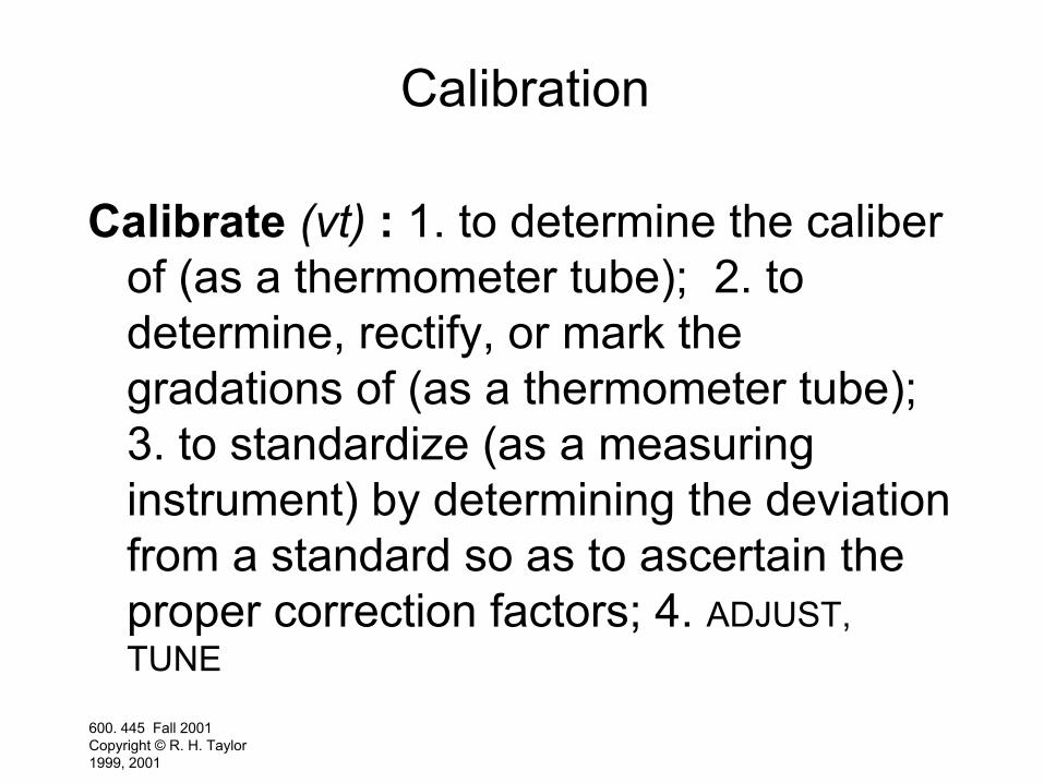
Calibration
Calibrate (vt) : 1. to determine the caliber of (as a thermometer tube); 2. to determine, rectify, or mark the gradations of (as a thermometer tube); 3. to standardize (as a measuring instrument) by determining the deviation from a standard so as to ascertain the proper correction factors; 4. ADJUST, TUNE

600. 445 Fall 2001Copyright © R. H. Taylor 1999, 2001
Calibration
Reality
Measuring device
Model of Reality
+
-Error

600. 445 Fall 2001Copyright © R. H. Taylor 1999, 2001
Calibration
Reality
Actuation device
Model of Reality
+
-Error

600. 445 Fall 2001Copyright © R. H. Taylor 1999, 2001
Basic Techniques
• Parameter Estimation
• Mapping the space
600. 445 Fall 2001Copyright © R. H. Taylor 1999, 2001
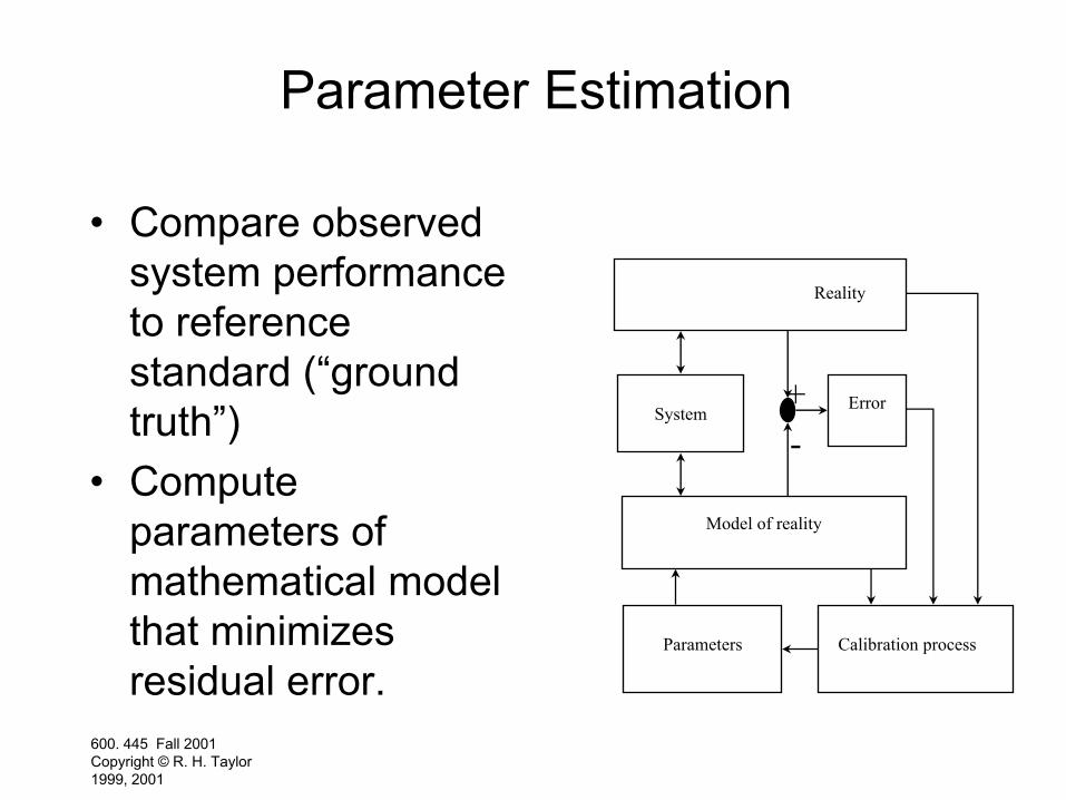
Parameter Estimation
• Compare observed system performance to reference standard (“ground truth”)
• Compute parameters of mathematical model that minimizes residual error.
Reality
System
Model of reality
+-
Error
Parameters Calibration process

600. 445 Fall 2001Copyright © R. H. Taylor 1999, 2001
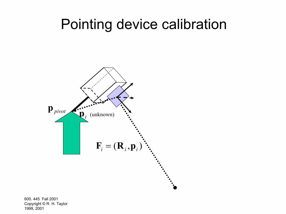
Pointing device calibration
F R pi i i= ( , )
p t (unknown)p pivot
600. 445 Fall 2001Copyright © R. H. Taylor 1999, 2001
Pointing device calibration
F R pi i i= ( , )
p t (unknown)p pivot

600. 445 Fall 2001Copyright © R. H. Taylor 1999, 2001
Pointing device calibration
F R pi i i= ( , )
tpp pivot
600. 445 Fall 2001Copyright © R. H. Taylor 1999, 2001
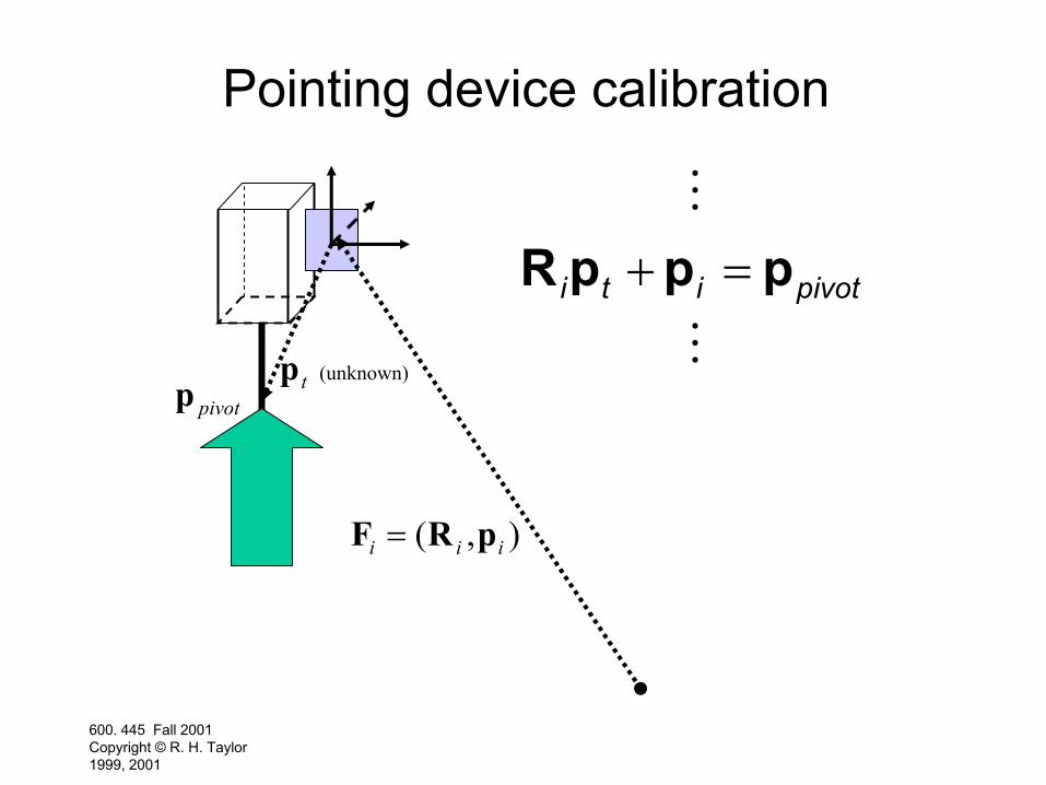
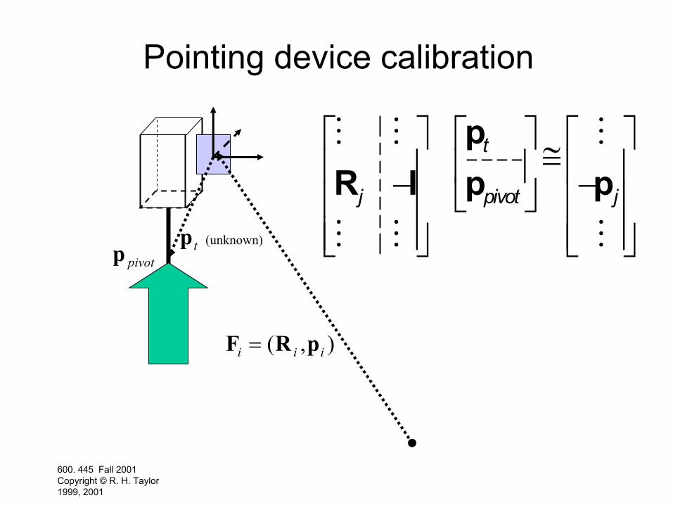
Pointing device calibration
i t i pivot+ =R p p p
F R pi i i= ( , )
p t (unknown)p pivot
600. 445 Fall 2001Copyright © R. H. Taylor 1999, 2001
Pointing device calibration
t
j pivot j
≅ − −
pR I p p
F R pi i i= ( , )
p t (unknown)p pivot
600. 445 Fall 2001Copyright © R. H. Taylor 1999, 2001
Linear Parameter Estimation
p f q q
p f q q
f q q
f q q qf
nom n
i
jn
q q
fq
q
q
J
= =
= +
≈ +∂∂
L
N
MMMM
O
Q
PPPP
L
NMMM
O
QPPP
≡ +
( ) [ ,...
( )
( ) ( )
( ) ( )
where ] are parametersT
*
1
1
∆
∆
∆
∆
600. 445 Fall 2001Copyright © R. H. Taylor 1999, 2001
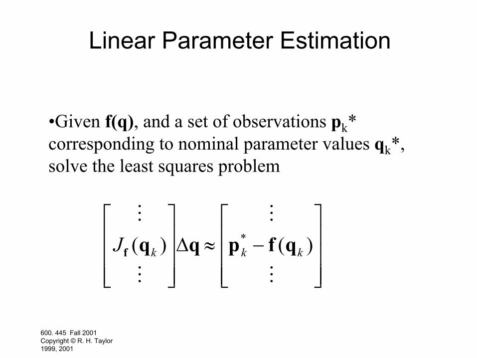
Linear Parameter Estimation
•Given f(q), and a set of observations pk* corresponding to nominal parameter values qk*, solve the least squares problem
J k k kf q q p f q( ) ( )*L
NMMM
O
QPPP
≈ −L
NMMM
O
QPPP
∆

600. 445 Fall 2001Copyright © R. H. Taylor 1999, 2001
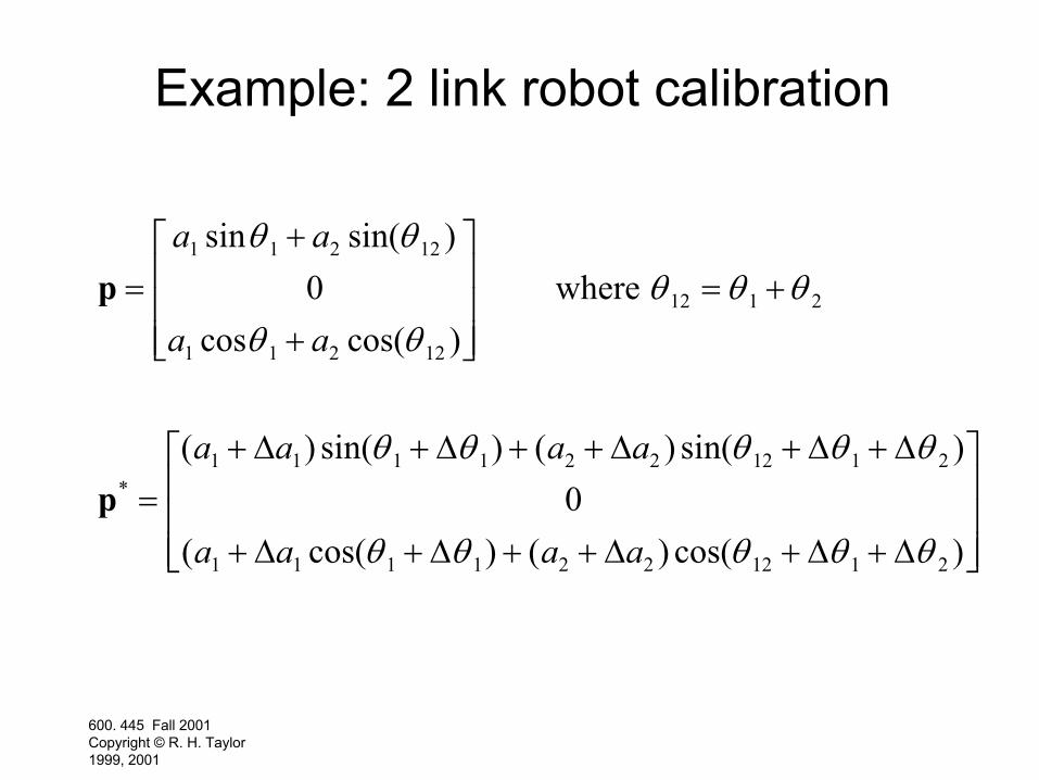
Example: 2 link robot calibration
*kp
1a
2a
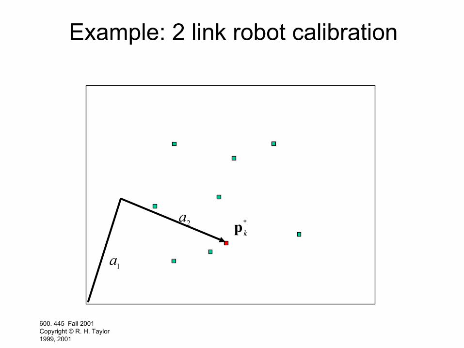
600. 445 Fall 2001Copyright © R. H. Taylor 1999, 2001
Example: 2 link robot calibration
*kp
1a
2a
600. 445 Fall 2001Copyright © R. H. Taylor 1999, 2001
Example: 2 link robot calibration
p
p
=+
+
L
NMMM
O
QPPP
= +
=+ + + + + +
+ + + + + +
L
NMMM
O
QPPP
a a
a a
a a a a
a a a a
1 1 2 12
1 1 2 12
12 1 2
1 1 1 1 2 2 12 1 2
1 1 1 1 2 2 12 1 2
0
0
sin sin( )
cos cos( )
( ) sin( ) ( ) sin( )
( cos( ) ( ) cos( )
*
θ θ
θ θθ θ θ
θ θ θ θ θ
θ θ θ θ θ
where
∆ ∆ ∆ ∆ ∆
∆ ∆ ∆ ∆ ∆

600. 445 Fall 2001Copyright © R. H. Taylor 1999, 2001
Example: 2 link robot calibration
p f q f
f q f q f q f q py
k k
k k
k k
k k k k k
a aa a
a a
a a
aa a Rot
= = =+
+
L
NMMM
O
QPPP
= +
∂∂
∂∂
∂∂
∂∂
L
N
MMMM
O
Q
PPPP
L
N
MMMM
O
Q
PPPP≈ −
( ) ( , , , )sin sin( )
cos cos( )
( ) ( ) ( ) ( )( ,
, ,
, ,
* ,
1 2 1 2
1 1 2 12
1 1 2 12
12 1 2
1 2 1 2
1
2
1
2
1 1
0θ θθ θ
θ θθ θ θ
θ θ θθ
θ
where
so we solve the least squares problem
∆∆∆∆
k
ka Rot)
( , ),+LNM
OQP
L
N
MMMMM
O
Q
PPPPP2 1y θ

600. 445 Fall 2001Copyright © R. H. Taylor 1999, 2001
Example: 2 link robot calibration
Here
so
Ja a
a a
a aa a
aa
k
k k k k k
k k k k k
k k k k k
k k k k k
f q( )sin sin (cos cos ) cos
cos cos (sin sin ) cos
sin sin (cos cos ) coscos cos (sin sin ) cos
, , , , ,
, , , , ,
, , , , ,
, , , , ,
=+
− + −
L
NMMM
O
QPPP
+− + −
L
N
MMMM
O
Q
PPPP
θ θ θ θ θ
θ θ θ θ θ
θ θ θ θ θθ θ θ θ θ θ
θ
1 12 1 1 12 2 12
1 12 1 1 12 2 12
1 12 1 1 12 2 12
1 12 1 1 12 2 12
1
2
1
0 0 0 0
∆∆∆∆ 2
1 1 2 12
1 1 2 12
L
N
MMMM
O
Q
PPPP≈
− +− +
L
N
MMMM
O
Q
PPPPx a az a ak k k
k k k
*, ,
*, ,
sin sin( )cos cos( )
θ θθ θ

600. 445 Fall 2001Copyright © R. H. Taylor 1999, 2001

600. 445 Fall 2001Copyright © R. H. Taylor 1999, 2001
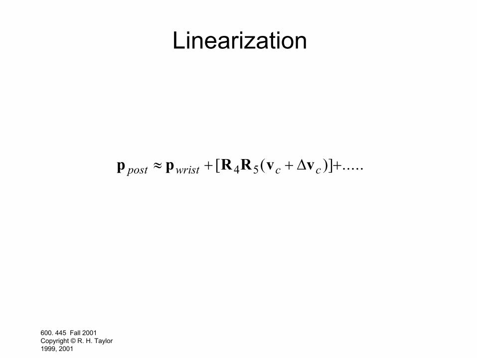
Example: Robodoc Wrist Calibration
• Basic robot had very accurate calibration
• Custom wrist was less accurate
• Crucial goal was to determine position of cutter tip
Cutter
Calibration post
600. 445 Fall 2001Copyright © R. H. Taylor 1999, 2001

600. 445 Fall 2001Copyright © R. H. Taylor 1999, 2001
Kinematic Model
p p R z x vtool wrist distal= + + • +( , ) ( )θ θ α4 4∆
v R x R y v vdistal c c= • + +( , ) [ ( , )( )]β θ θ5 5∆ ∆
600. 445 Fall 2001Copyright © R. H. Taylor 1999, 2001
Linearization
p p R R v vpost wrist c c≈ + + +[ ( )] .....4 5 ∆

600. 445 Fall 2001Copyright © R. H. Taylor 1999, 2001
Linear Least Squares
• Most commonly used method for parameter estimation
• Many numerical libraries
• See the web site• Here is a quick
review
Microsoft PowerPoint Presentation
600. 445 Fall 2001Copyright © R. H. Taylor 1999, 2001
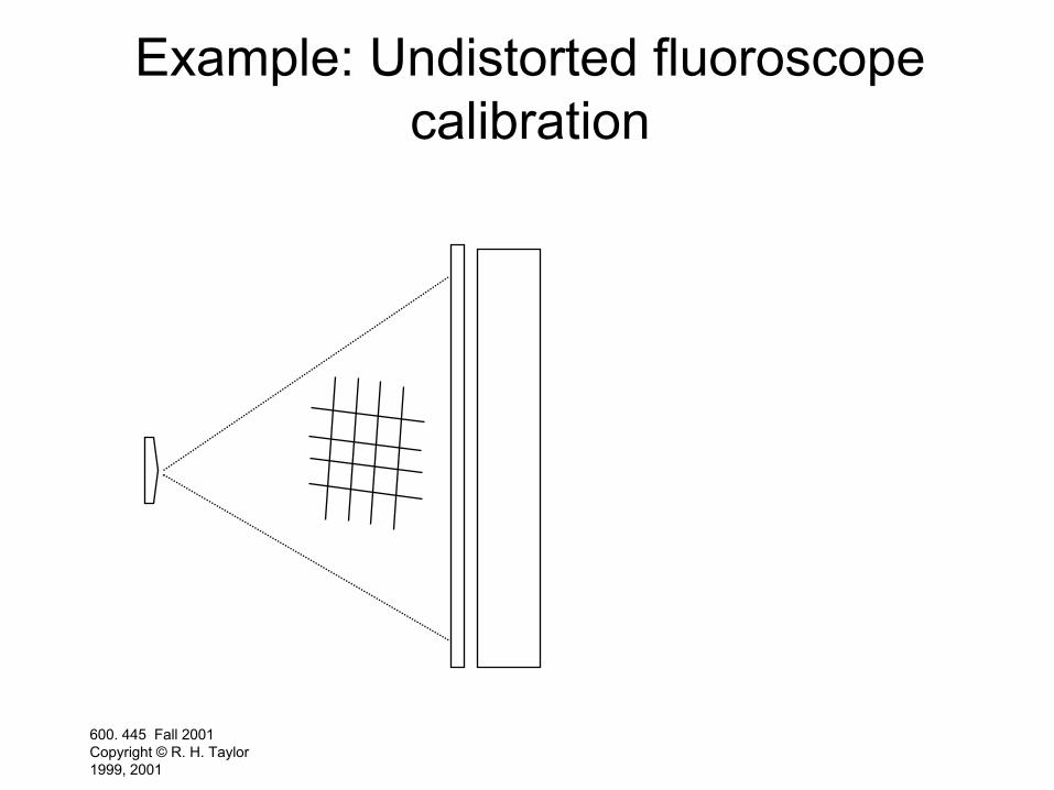
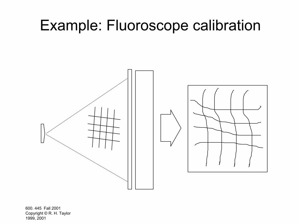
Example: Undistorted fluoroscope calibration

600. 445 Fall 2001Copyright © R. H. Taylor 1999, 2001
Calibration if no distortion (version 1)
{ }0 1
Assume no distortion. For the moment alsoassume that you have N point calibrationfeatures (e.g., small steel balls) at knownpositions , , relative to the detector.Assume further that the points
N−a a
{ }0 1
create imagesat corresponding points , , on the detector. Estimate the position of the x-raysource relative to the detector
N−d ds
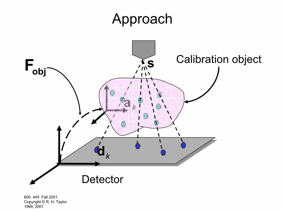
600. 445 Fall 2001Copyright © R. H. Taylor 1999, 2001
Approach
s
kd
ka
Calibration objectobjF
Detector
600. 445 Fall 2001Copyright © R. H. Taylor 1999, 2001
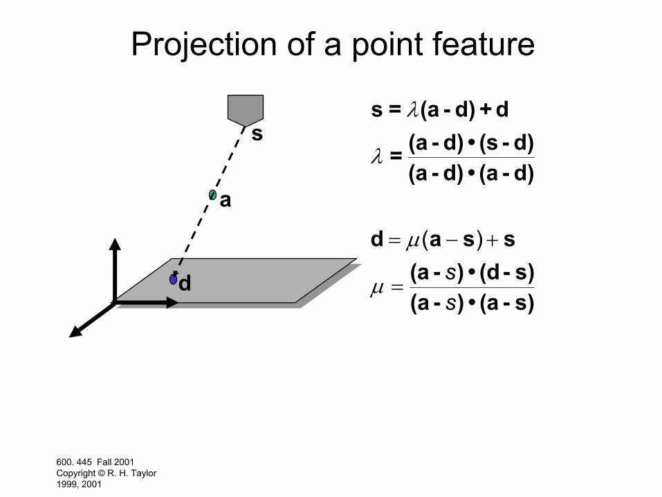
Projection of a point feature
s
d
a
( )ss
λ
λ
µ
µ
= − +
=
s = (a - d) + d(a - d) • (s - d)=(a - d) • (a - d)
d a s s(a - ) • (d - s)(a - ) • (a - s)
600. 445 Fall 2001Copyright © R. H. Taylor 1999, 2001
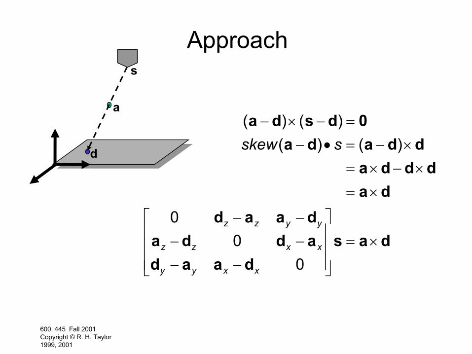
Approachs
d
a( ) ( )
( ) ( )
00
0
z z y y
z z x x
y y x x
skew s− × − =
− • = − ×= × − ×= ×
− − − − = × − −
a d s d 0a d a d d
a d d da d
d a a da d d a s a dd a a d

600. 445 Fall 2001Copyright © R. H. Taylor 1999, 2001
Approach
s
d
a
0 0 0 0
1 1 1 1
Solve least squares problem
( )
( )
x
y
z
N N N N
skew
skew − − − −
− × ≅
− ×
sa d a dss
a d a d

600. 445 Fall 2001Copyright © R. H. Taylor 1999, 2001
What if pose of calibration object is imprecisely known?
• This is a hairier problem, but solvable• In fact, it makes a great homework
assignment ….
600. 445 Fall 2001Copyright © R. H. Taylor 1999, 2001
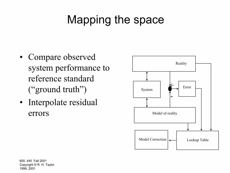
Mapping the space
• Compare observed system performance to reference standard (“ground truth”)
• Interpolate residual errors
Reality
System
Model of reality
+-
Error
Lookup TableModel Correction
600. 445 Fall 2001Copyright © R. H. Taylor 1999, 2001
Example: Fluoroscope calibration

600. 445 Fall 2001Copyright © R. H. Taylor 1999, 2001
Projection of a point feature with distortion
s
u
a
λ
λ
s = (a - d) + d(a - d) • (s - d)=(a - d) • (a - d)
d
ν= ( , )u f d

600. 445 Fall 2001Copyright © R. H. Taylor 1999, 2001

600. 445 Fall 2001Copyright © R. H. Taylor 1999, 2001
600. 445 Fall 2001Copyright © R. H. Taylor 1999, 2001
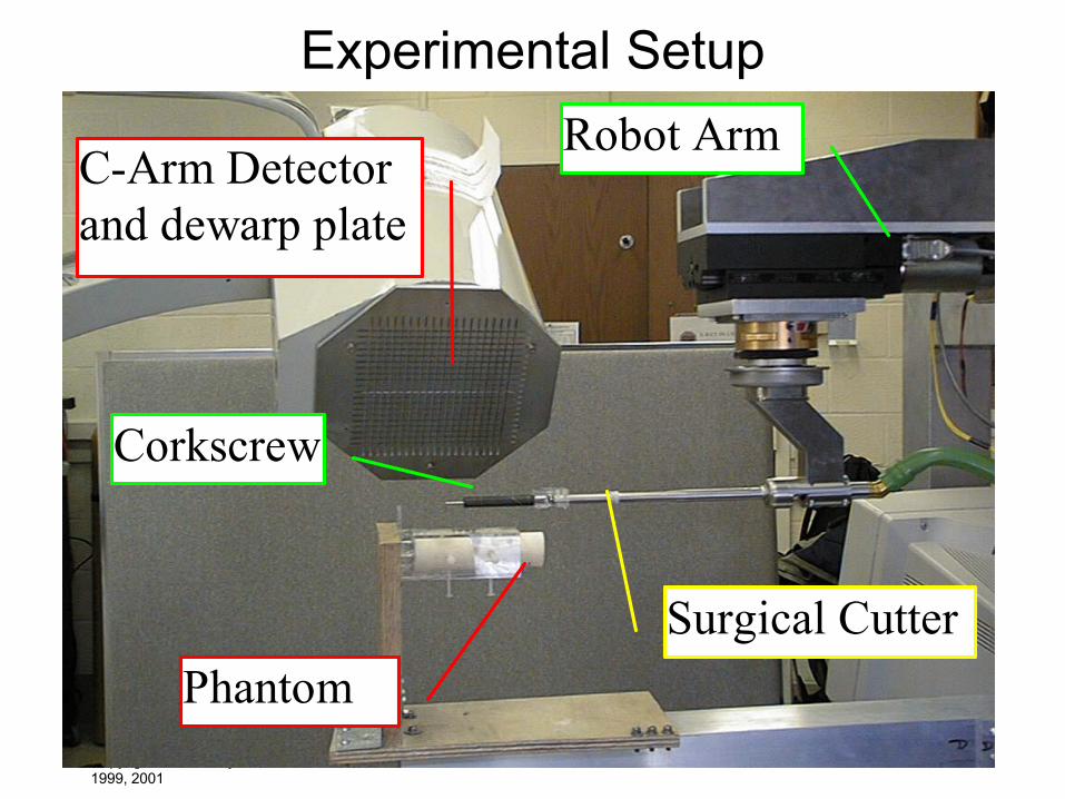
Experimental Setup
C-Arm Detectorand dewarp plate
Robot Arm
Surgical Cutter
Corkscrew
Phantom
600. 445 Fall 2001Copyright © R. H. Taylor 1999, 2001
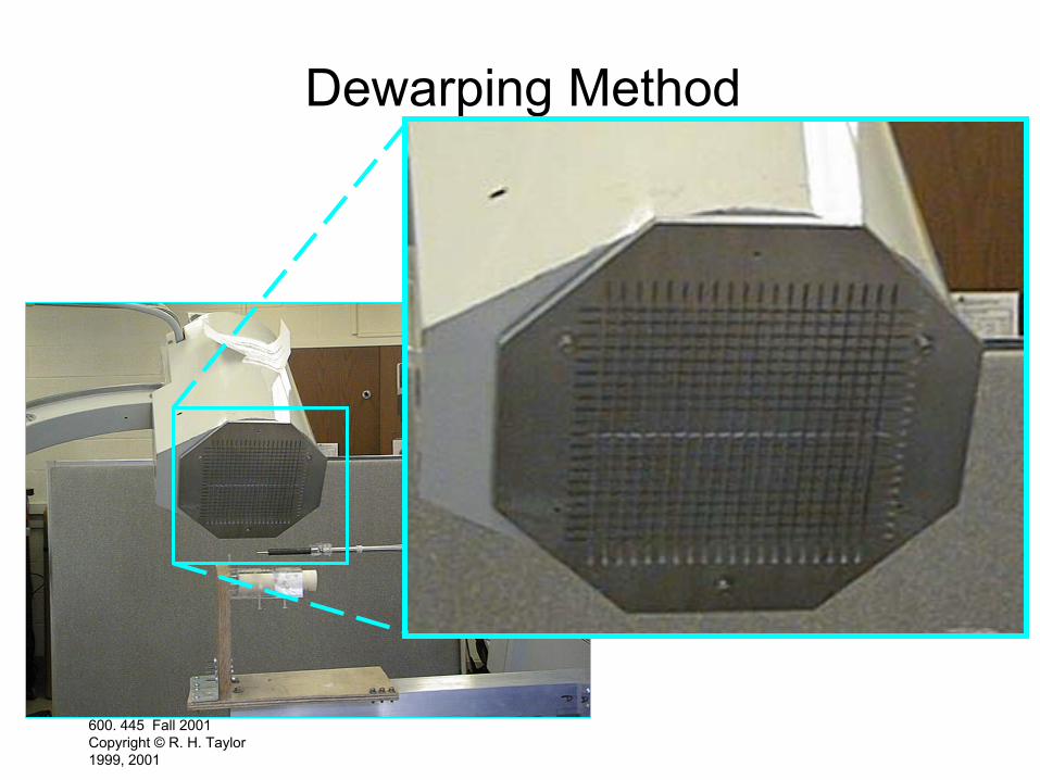
Dewarping Method
600. 445 Fall 2001Copyright © R. H. Taylor 1999, 2001
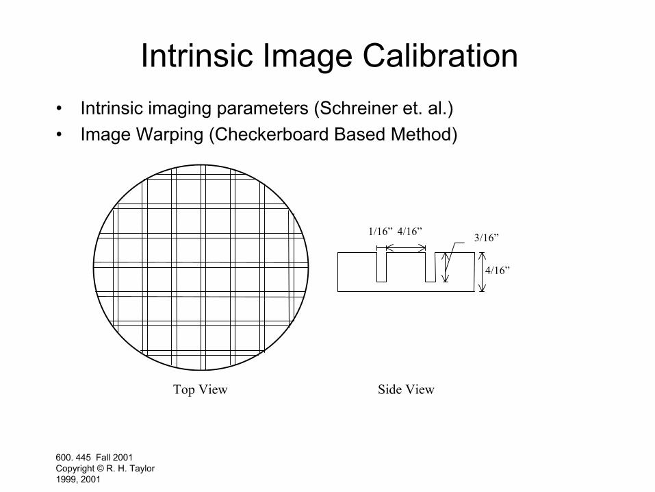
Intrinsic Image Calibration• Intrinsic imaging parameters (Schreiner et. al.)• Image Warping (Checkerboard Based Method)
4/16”1/16” 3/16”
4/16”
Top View Side View

600. 445 Fall 2001Copyright © R. H. Taylor 1999, 2001
Step 0: Acquire Image
600. 445 Fall 2001Copyright © R. H. Taylor 1999, 2001
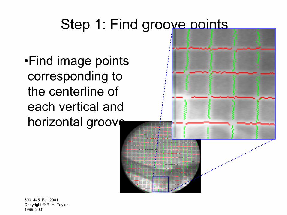
Step 1: Find groove points
•Find image points corresponding to the centerline of each vertical and horizontal groove
600. 445 Fall 2001Copyright © R. H. Taylor 1999, 2001
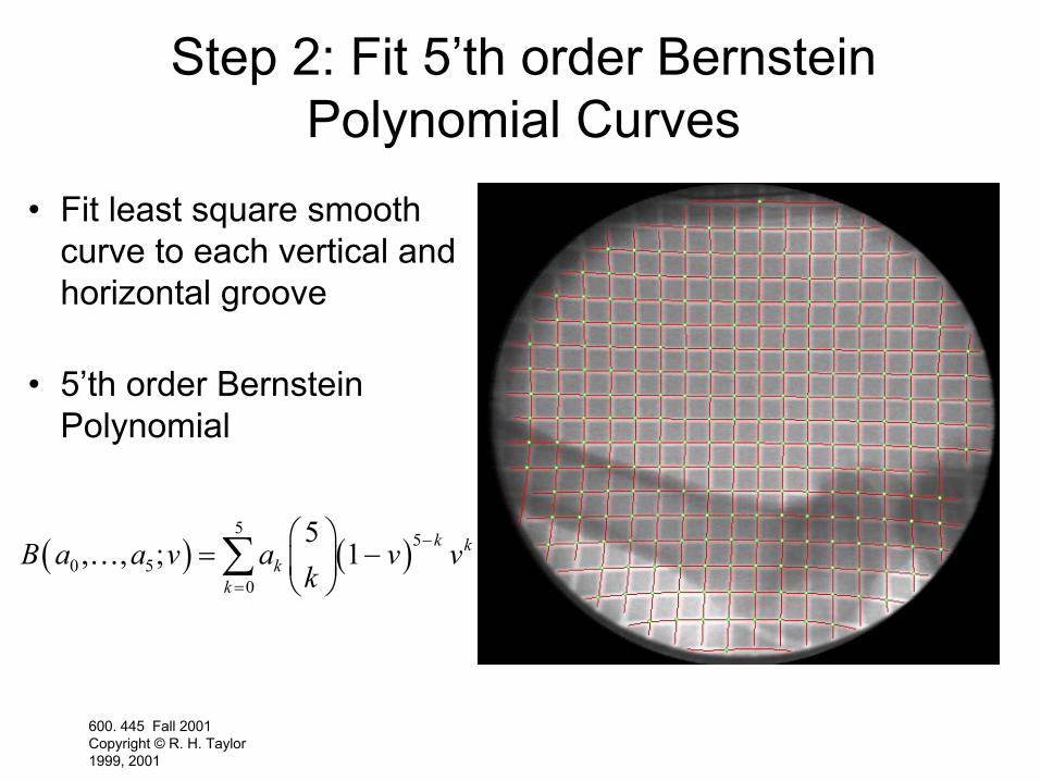
Step 2: Fit 5’th order Bernstein Polynomial Curves
• Fit least square smooth curve to each vertical and horizontal groove
• 5’th order Bernstein Polynomial
( ) ( )5
50 5
0
5, , ; 1 k k
kk
B a a v a v vk
−
=
= −
∑…

600. 445 Fall 2001Copyright © R. H. Taylor 1999, 2001
Step 3: Dewarp
• Employ a two pass scan line algorithm to dewarp the image

600. 445 Fall 2001Copyright © R. H. Taylor 1999, 2001
Advantages
• Fast– ≈ 2 seconds on Pentium II 400
• Robust– works well even with overlaid objects
• Sub-pixel Accuracy– mean error 0.12 mm on the central area
• Does not completely obscure the image– trades off image contrast depth for image area
600. 445 Fall 2001Copyright © R. H. Taylor 1999, 2001
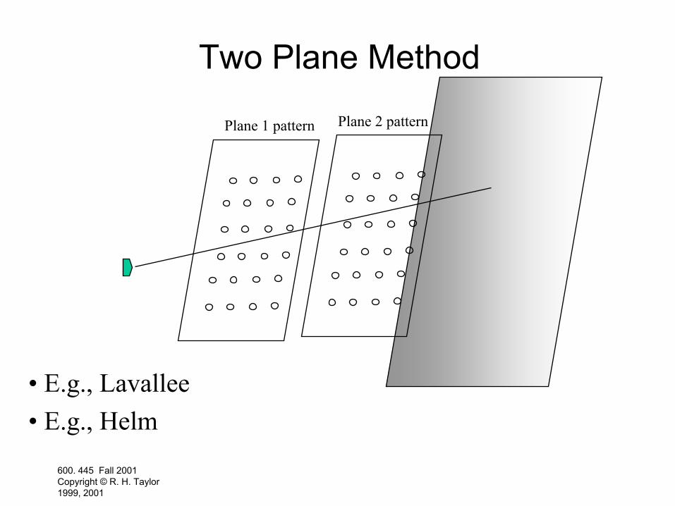
Two Plane Method
Plane 1 pattern Plane 2 pattern
• E.g., Lavallee• E.g., Helm
600. 445 Fall 2001Copyright © R. H. Taylor 1999, 2001
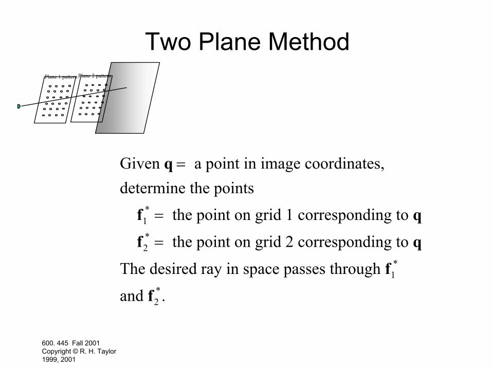
Two Plane MethodPlane 1 pattern Plane 2 pattern
Given a point in image coordinates,determine the points the point on grid 1 corresponding to
the point on grid 2 corresponding to
The desired ray in space passes through
and
q
f qf q
ff
=
=
=1
2
1
2
*
*
*
*.

600. 445 Fall 2001Copyright © R. H. Taylor 1999, 2001
Photos: Sofamor Danek
600. 445 Fall 2001Copyright © R. H. Taylor 1999, 2001
Interpolation
• Ubiquitous throughout CIS research and applications
• Many techniques and methods
• Here are a few more notes
Microsoft PowerPoint Presentation
600. 445 Fall 2001Copyright © R. H. Taylor 1999, 2001
Two plane calibration• Again, the essential problem is to
determine the coordinates in the two planes at which the source-to-detector ray passes through the plane.
• Many methods for this. E.g., – Find the four surrounding bead locations
on each plane and use bilinear interpolation
– Fit a general spline model for the distortion on each plane and then directly interpolate