The University of Manchester Research

A calibration method for non-positive definite covariancematrix in multivariate data analysisDOI:10.1016/j.jmva.2017.03.001

Document VersionAccepted author manuscript

Link to publication record in Manchester Research Explorer

Citation for published version (APA):Huang, C., Farewell, D., & Pan, J. (2017). A calibration method for non-positive definite covariance matrix inmultivariate data analysis. Journal of Multivariate Analysis. https://doi.org/10.1016/j.jmva.2017.03.001

Published in:Journal of Multivariate Analysis

Citing this paperPlease note that where the full-text provided on Manchester Research Explorer is the Author Accepted Manuscriptor Proof version this may differ from the final Published version. If citing, it is advised that you check and use thepublisher's definitive version.

General rightsCopyright and moral rights for the publications made accessible in the Research Explorer are retained by theauthors and/or other copyright owners and it is a condition of accessing publications that users recognise andabide by the legal requirements associated with these rights.

Takedown policyIf you believe that this document breaches copyright please refer to the University of Manchester’s TakedownProcedures [http://man.ac.uk/04Y6Bo] or contact uml.scholarlycommunications@manchester.ac.uk providingrelevant details, so we can investigate your claim.

Download date:24. Dec. 2019

A calibration method for non-positive definite

covariance matrix in multivariate data analysis

Chao Huang 1, Daniel Farewell 2 and Jianxin Pan 3∗

1 South East Wales Trials Unit, Cardiff University

Heath Park, Cardiff, CF14 4YS, UK2 Division of Population Medicine, School of Medicine, Cardiff University

Heath Park, Cardiff, CF14 4YS, UK3 School of Mathematics, University of Manchester,

Manchester M13 9PL, UK

Abstract

Covariance matrices that fail to be positive definite arise often in covari-ance estimation. Approaches addressing this problem exist, but are not wellsupported theoretically. In this paper, we propose a unified statistical andnumerical matrix calibration, finding the optimal positive definite surrogatein the sense of Frobenius norm. The proposed algorithm can be directly ap-plied to any estimated covariance matrix. Numerical results show that thecalibrated matrix is typically closer to the true covariance, while making onlylimited changes to the original covariance structure.

Keywords:Covariance matrix calibration, Nearness problem, Non-positive definiteness,Spectral decomposition

1. Introduction

The estimation of covariance matrices plays an essential role in multivari-able data analysis. Covariances are required by many statistical modellingapproaches, including multivariate regression and the analysis of spatial data.

∗Corresponding author. Tel: +44 161 2755864; Fax: +44 161 275 5819.Email Addresses: HuangC12@cardiff.ac.uk (C. Huang); farewelld@cf.ac.uk (D. Farewell);Jianxin.Pan@manchester.ac.uk (J. Pan)

Preprint submitted to Elsevier March 1, 2017

Often, well-estimated covariance matrices improve efficiency in estimatingparameters in a mean function [22]. In some circumstances, the covariancematrix may itself be of direct scientific interest: for instance, in spatial vari-ation analysis for geographical data, and in volatility analysis for financialdata.

However, it is not uncommon that estimators of covariance matrices failto be positive definite. A typical example is the sample covariance matrix,which is often singular when the sample size is close to, or less than, thedimension of the random samples [3]. If singularity is caused by collinear-ity, conventional ridge regression [18] or modern variable selection [6, 21]approaches may solve the problem by excluding redundant variables. Di-mension reduction approaches such as Principle Component Analysis [19]can also help to exclude eigenvalues with ignorable contributions.

However, these resolutions only apply in cases where such redundancetruly exists. More often, non-positive definiteness may be put down to thegeneric difficulty of maintaining positive definiteness in covariance estima-tion; resulting estimators may not even be positive semidefinite. Even forelaborately designed statistical approaches, the estimators of covariance ma-trices can be ill-conditioned [5, 14]. A number of approaches have beenproposed to resolve this issue. However, these are either limited to specialcircumstances or lack theoretical support. For instance, one alternative is touse the Moore-Penrose inverse of a non-positive definite matrix to replacethe regular inverse typically used in statistical inferences [20]. However, thisdoes not directly resolve the non-positive definiteness, and is lack of statisti-cal interpretation. Alternatively, a smoothing approach exists [23] in whichnon-positive eigenvalues of the covariance matrix estimator are replaced bycertain positive values. However, justification for the selection of these posi-tive values was scant.

Based on the fundamental work of Halmos [7], Higham [9] proposed asolution for finding the nearest (in the sense of Frobenius norm) positivesemidefinite matrix to an arbitrary input matrix. However, this surrogatepositive semidefinite matrix is still singular [9, 10], so difficulty persists inusing the surrogate matrix in statistical practice. Rebonto and Jackel [17]considered a correlation matrix calibration using the hyperspherical decom-position and eigenvalue correction, which again leads to positive semidefinitecorrelation matrices. Hendrikse et al.[8] proposed an eigenvalue correctionmethod using bootstrap resampling in order to reduce the bias arising insample eigenvalues. Their work focused on the correction of the sample

2

covariance, where the performance of the correction method relies on theassumed distribution of the covariance matrix eigenvalues in the population.

In this paper, we propose a unified approach to calibrate a non-positivedefinite covariance matrix to ensure positive definiteness. The calibrated co-variance matrix is usually closer to the true covariance matrix than the orig-inal covariance matrix estimator. Our proposed approach is implementedthrough a straightforward screening algorithm. In Section 2, we briefly re-view the matrix nearness problem, before proposing our novel calibrationmethod together with its integrated criterion and algorithm. In Section 3we conduct two simulation studies, and in Section 4 we discuss two casestudies, including a calibration of the non-positive definite covariance matrixobtained by nonparametric regression in Diggle and Verbyla [5]. Conclusionsare presented in Section 5.

2. Calibration method

2.1. The matrix nearness problem

In numerical analysis, a nearness problem involves finding, for a givenmatrix and a particular matrix norm, the nearest matrix that has certainimportant properties. Examples include finding the nearest covariance ma-trix [9] or correlation matrix [2, 16] in the sense of the Frobenius norm (or2-norm).

Given an arbitrary square matrix X of order n, we denote its Frobeniusnorm by ‖X‖ = trace(X⊤X)1/2. The nearness problem involves finding thenearest symmetric positive semidefinite matrix P0(X):

P0(X) = argminA≥0

‖X − A‖ (1)

Throughout, we shall assume that A ≥ 0 denotes both non-negative definite-ness and symmetry A = A⊤. Higham [9] used a polar decomposition to showthat the solution to (1) has the explicit form P0(X) = (B + H)/2, whereB = S(X) = (X +X⊤)/2 is the symmetric matrix version of X , and H isthe symmetric polar factor of B, satisfying B = UH with U a unitary ma-trix and H ≥ 0. This solution has been compiled in a MATLAB file namedpoldex.m, which can be found in the Matrix Computation Toolbox [11].Clearly, if X is symmetric then the solution becomes P0(X) = (X + H)/2.If, further, we are given the spectral decomposition of a symmetric X = X⊤

(that is, X = QΛQ⊤ for Q⊤Q = I and Λ = diag(λ1, . . . , λn)), we have

3

P0(X) = Qdiag{max(λ1, 0), . . . ,max(λn, 0)}Q⊤. In other words, the nearestpositive semidefinite matrix P0(X) can be obtained by replacing by zero anynegative eigenvalues of a symmetric X [10], eliminating the correspondingcolumns of Q (and causing some information loss). A immediate alternativeis to instead replace negative eigenvalues by positive values, so that a positivedefinite correction of X is formed without this loss of information about Q.However, the theory of this idea need to be justified, particularly on how tochoose appropriate replacement positive values, for which we will address inthis paper.

2.2. A new calibration approach

We now aim to find a positive definite matrix surrogate for a genericX . First, we formulate this question as a nearness problem. For c ≥ 0,let Dc = {A : A − cI ≥ 0} be the set of positive definite matrices with noeigenvalue smaller than c. Given X , finding the nearest matrix Pc(X) ∈ Dc

to X in terms of the Frobenius norm amounts to defining

Pc(X) = argminA∈Dc

‖X − A‖. (2)

An explicit expression for Pc(X) is given in Theorem 1.

Theorem 1. Given X and a constant c ≥ 0, the nearest (in the sense ofFrobenius norm) matrix Pc(X) ∈ Dc to X is of the form

Pc(X) = P0(X − cI) + cI (3)

where (as before) P0(X − cI) = (B + H)/2 for B = S(X − cI) and H thepolar factor of B. Furthermore, if X is symmetric with spectral decompositionX = Qdiag(λ1, . . . , λn)Q

⊤ then Pc(X) has the simplified form

Pc(X) = Qdiag{max(λ1, c), . . . ,max(λn, c)}Q⊤. (4)

Proof: The details of the proof are deferred to the Appendix. �

Maintaining symmetry in covariance estimation is typically not difficult,so direct use of (4) will often be sufficient in practice. For non-symmetricX , one may directly symmetrize X before calibration. Note that Pc(X) onlydepends on X via its symmetric version S(X), so (4) can equivalently beapplied to S(X).

4

2.3. Selection criterion

Clearly Pc(X) varies with c and, as c decreases, the domain Dc of Aexpands. At c = 0, Pc(X) = P0(X) becomes positive semidefinite (unless, ofcourse, all eigenvalues of X are already positive). Consequently, we requirea criterion for selecting an appropriate positive value, c = c∗, say. Let λ+

min

be the smallest positive eigenvalue of an estimated covariance matrix X .In order to maintain, as far as possible, the covariance structure of X , it isreasonable to constrain 0 ≤ c∗ ≤ λ+

min. Rather than make simple choices suchas c∗ = λ+

min/2, here we propose a tuning approach, balancing proximity toX with proximity to singularity. Writing cα = 10−αλ+

min, where α ≥ 0 is atuning parameter, with c0 = λ+

min and c∞ = 0 (i.e., c → 0 as α → ∞), wechoose c∗ as follows:

Definition 1. Define c∗ = cα∗via

α∗ = argminα

‖X − Pcα(X)‖+ α, (5)

where (as before) cα = 10−αλ+min.

Rather than simply minimize the quantity ‖X − A‖, in (5) we also adda penalty (namely, α) that penalises small values of c. Such penalty termsare widely used in a variety of statistical contexts, such as the AIC/BIC andpenalty functions [1, 6, 21]. Reassuringly, positive definite covariance matri-ces remain unchanged after calibration. To see this, note that Pλ+

min(X) = X

if X is itself positive definite. In this case, choosing α = 0 (so c = λ+min)

thus makes both ‖X − Pcα(X)‖ and α vanish, so c∗ = λ+min and the solution

P∗(X) = Pc∗(X) completely reduces to X .The tuning parameter α can also be interpreted in terms of the condition

number of the matrix Pcα(X) [24, p146]. For a positive semi-definite matrix,the condition number is the ratio of its biggest to smallest eigenvalues. Thecondition number can warn us the numerical inaccuracy in calculating theinverse of a given matrix. In our case, let λ+

max be the biggest positive eigen-values of X and d = λ+

max/λ+min. Then the condition number of the calibrated

matrix Pcα(X) is κ(Pcα(X)) = 10αd. Therefore, the penalty α approximatesthe number of digits of accuracy we are prepared to sacrifice in the inversionof Pcα(X) in order to reduce ‖X − Pcα(X)‖.

5

2.4. Algorithm

In practice, we implement a screening-search strategy for the tuning pa-rameter α. Rather than let α ∈ [0,+∞), we constrain the screening to afeasible region. This strategy is employed in the following algorithm.

Step 1. Given a feasible region of α, say [0, αN ], create a partition 0 =α0 < α1 < α2 < . . . < αN . For α ∈ {α0, . . . , αN}, compute the correspondingcα and use (4) to calculate the resulting solution matrix Pcα(X). We choose

α∗ = argminα∈{α0,...,αN}

‖X − Pcα(X)‖+ α. (6)

Step 2. Set c∗ = cα∗, and return P∗(X) = Pc∗(X) as the final calibrated

covariance matrix.

In terms of the screening region [0, αN ] and its partition, we make thefollowing recommendations. In most applications, 10−α become negligiblewhen α > 10, so we take our default option to be αN = 10. Options oflarger αN are possible when the original λ+

min is in large scale. However, wewould not recommend a too large αN , as it corresponds to a large conditionnumber of P∗(X). When screening α ∈ [0, αN ], we suggest a uniform parti-tion of the region: for example, given αN = 10, we could use the partition0, 1, . . . , 10 or 0, 0.5, . . . , 10. More refined partition would be preferable whenextra accuracy in calibration is demanded.

3. Simulation studies

In this section, we carry out two simulation studies to assess the per-formance of our proposed calibration method. In Simulation 1, we considerthree commonly used covariance structures: compound symmetry, first-orderautoregressive (ar(1)) and tri-diagonal. In Simulation 2, a more general co-variance structure formed by the modified Cholesky decomposition [15] isinvestigated. Covariance matrices are fitted via the nonparametric covari-ance estimation approach of Diggle and Verblya [5]. The advantage of thatapproach lies in that the variogram considered therein has a clear statisticalinterpretation, being useful in describing spatial correlation in geo-statistics[4], and in judging if the covariance structure is stationary. Here we focus onthe non-positive definite covariance matrices obtained by that approach toassess the performance of the proposed calibration method.

6

The longitudinal data we consider here are described by (yij, tij), i =1, . . . , n, j = 1, . . . , ni, where yij represents the measurement j (out of ni)on subject i and tij is its measurement time. Let µij = µi(tij) be the meanof yij and µi = (µi1, . . . , µini

)⊤ be the vector of the means of the responsesyi = (yi1, . . . , yini

)⊤. Assume Σi is the covariance matrix of the responsesyi, where the elements of Σi are defined by a generic covariance function(Σi)j,k = Σ(tij , tik). Following [5], a multivariate normal distribution is as-sumed, i.e., yi ∼ N (µi,Σi). The main covariance fitting process of [5] isbriefly summarized as follows. Firstly, a local polynomial smoothing tech-

nique is used to estimate the variances in Σi, (Σi)j,j, using the sample vari-

ances (yij − µij)2, j = 1, . . . , ni, where µij are the fitted means through cer-

tain nonparametric regression estimation methods, such as [25]. Secondly,a bivariate local polynomial smoothing method is used to model the var-iograms vijk through the sample variograms {(yij − µij) − (yik − µik)}

2/2.

Finally, the off-diagonal elements of Σi, (Σi)j,k, j 6= k, are estimated through

(Σi)j,k = {(Σi)j,j + (Σi)k,k}/2− vijk.

3.1. Simulation 1

We generate 100 datasets based on the Gaussian process mechanism de-scribed above. In each dataset there are n = 50 subjects and ni = m = 10 or20 repeated measurements for each subject. The means µij are formulatedas µij = tij + sin(tij) for all i, j, with measurement times tij = j for all j.Given a common variance σ2 and a correlation parameter ρ, the covariancestructure Σi of subject i is assumed to have the particular structure describedbelow:

1. Compound symmetry. Within-subject correlation is assumed equal forany disjoint pair of observations. In other words, Σi = σ2{(1−ρ)I+ρJ},where ρ ∈ (−1/(m − 1), 1), I is an identity matrix and J is a matrixof ones with order m.

2. ar(1). Within-subject correlation decreases with the time separationas Σi = σ2(ρ|j−k|) (j, k = 1, . . . , m, ρ ∈ (−1, 1)).

3. Tri-diagonal. Within-subject correlation vanishes except for adjacentobservations, i.e., the (j, k)-th element of Σi is given by

(Σi)j,k =

σ2, j = kσ2ρ, |j − k| = 10, |j − k| ≥ 2

7

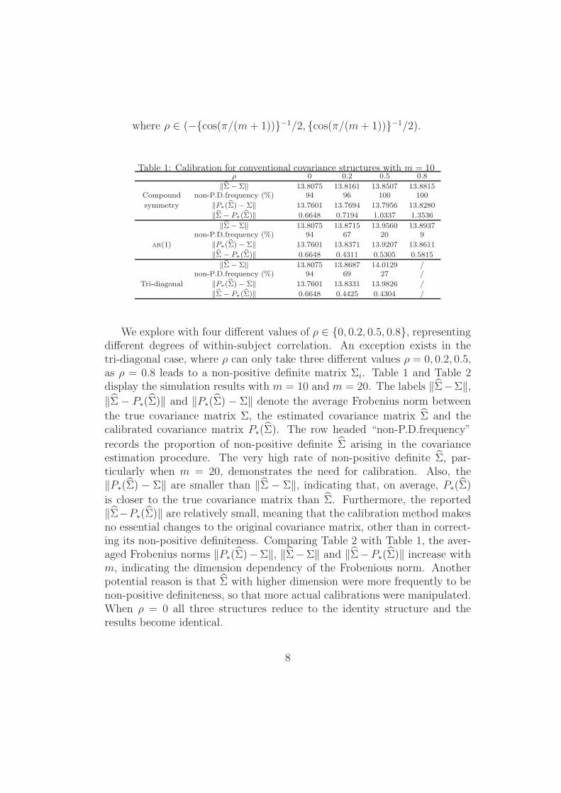
where ρ ∈ (−{cos(π/(m+ 1))}−1/2, {cos(π/(m+ 1))}−1/2).

Table 1: Calibration for conventional covariance structures with m = 10ρ 0 0.2 0.5 0.8

‖Σ−Σ‖ 13.8075 13.8161 13.8507 13.8815Compound non-P.D.frequency (%) 94 96 100 100

symmetry ‖P∗(Σ)− Σ‖ 13.7601 13.7694 13.7956 13.8280

‖Σ− P∗(Σ)‖ 0.6648 0.7194 1.0337 1.3536

‖Σ−Σ‖ 13.8075 13.8715 13.9560 13.8937non-P.D.frequency (%) 94 67 20 9

ar(1) ‖P∗(Σ)− Σ‖ 13.7601 13.8371 13.9207 13.8611

‖Σ− P∗(Σ)‖ 0.6648 0.4311 0.5305 0.5815

‖Σ−Σ‖ 13.8075 13.8687 14.0129 /non-P.D.frequency (%) 94 69 27 /

Tri-diagonal ‖P∗(Σ)− Σ‖ 13.7601 13.8331 13.9826 /

‖Σ− P∗(Σ)‖ 0.6648 0.4425 0.4304 /

We explore with four different values of ρ ∈ {0, 0.2, 0.5, 0.8}, representingdifferent degrees of within-subject correlation. An exception exists in thetri-diagonal case, where ρ can only take three different values ρ = 0, 0.2, 0.5,as ρ = 0.8 leads to a non-positive definite matrix Σi. Table 1 and Table 2display the simulation results with m = 10 and m = 20. The labels ‖Σ−Σ‖,

‖Σ − P∗(Σ)‖ and ‖P∗(Σ) − Σ‖ denote the average Frobenius norm between

the true covariance matrix Σ, the estimated covariance matrix Σ and thecalibrated covariance matrix P∗(Σ). The row headed “non-P.D.frequency”

records the proportion of non-positive definite Σ arising in the covarianceestimation procedure. The very high rate of non-positive definite Σ, par-ticularly when m = 20, demonstrates the need for calibration. Also, the‖P∗(Σ) − Σ‖ are smaller than ‖Σ − Σ‖, indicating that, on average, P∗(Σ)

is closer to the true covariance matrix than Σ. Furthermore, the reported‖Σ−P∗(Σ)‖ are relatively small, meaning that the calibration method makesno essential changes to the original covariance matrix, other than in correct-ing its non-positive definiteness. Comparing Table 2 with Table 1, the aver-aged Frobenius norms ‖P∗(Σ)−Σ‖, ‖Σ−Σ‖ and ‖Σ−P∗(Σ)‖ increase withm, indicating the dimension dependency of the Frobenious norm. Anotherpotential reason is that Σ with higher dimension were more frequently to benon-positive definiteness, so that more actual calibrations were manipulated.When ρ = 0 all three structures reduce to the identity structure and theresults become identical.

8

Table 2: Calibration for conventional covariance structures with m = 20ρ 0 0.2 0.5 0.8

‖Σ−Σ‖ 29.0470 29.2198 29.2109 29.3859Compound non-P.D.frequency (%) 100 100 100 100

symmetry ‖P∗(Σ)− Σ‖ 28.7750 29.0383 29.1101 29.3128

‖Σ− P∗(Σ)‖ 3.2369 2.0760 1.6720 1.6933

‖Σ−Σ‖ 29.0470 29.1571 29.3189 29.4197non-P.D.frequency (%) 100 100 100 74

ar(1) ‖P∗(Σ)− Σ‖ 28.7750 28.8966 29.1032 29.3403

‖Σ− P∗(Σ)‖ 3.2369 2.9150 2.1133 0.7128

‖Σ−Σ‖ 29.0470 29.0928 29.2723 /non-P.D.frequency (%) 100 100 100 /

Tri-diagonal ‖P∗(Σ)− Σ‖ 28.7750 28.8416 29.0362 /

‖Σ− P∗(Σ)‖ 3.2369 2.8607 2.5349 /

3.2. Simulation 2

We now consider a more general covariance structure via the modifiedCholesky decomposition [15]. With a covariance matrix Σi of order m, themodified Cholesky decomposition of Σi is specified by TiΣiT

⊤i = Di, where

Ti =

1 0 0 · · · 0−φi21 1 0 · · · 0−φi31 −φi32 1 · · · 0

......

.... . .

...−φim1 −φim2 −φim3 · · · 1

, Di =

σ2i1 0 · · · 00 σ2

i2 · · · 0...

.... . .

...0 0 · · · σ2

im

,

and where φijk and σ2ij are the generalized autoregressive parameters and

innovation variances, respectively. We then parameterize φijk and σ2ij as

functions of their corresponding measurement times, φijk = g(tij, tik) andln σ2

ij = q(tij), where g(., .) and q(.) are two- and one-dimensional smooth-ing functions, respectively. With different specifications for g(., .) and q(.),the covariance matrix Σi encompases a wide range of covariance structures.Here we assume g(tij, tik) = m−2(t2ij + t2ik) exp{−(tij − tik)/4} and q(tik) =2 ln[ln{tik/(m+2)}], with m = 10, 20. With the same mean function of Sim-ulation 1, 100 simulated datasets are generated. The numerical results arepresented in Table 3. Again, we see that our proposed method provides, onaverage, a closer-to-true surrogate covariance matrix. In the case of m = 20,the calibrated covariance matrix P∗(Σ) substantially improves Σ in the sense

of the Frobenius norm (‖P∗(Σ) − Σ‖ = 36.5162 while ‖Σ − Σ‖ = 45.5746).

Comparing the case ofm = 10 tom = 20, ‖Σ−P∗(Σ)‖ substantially increases

9

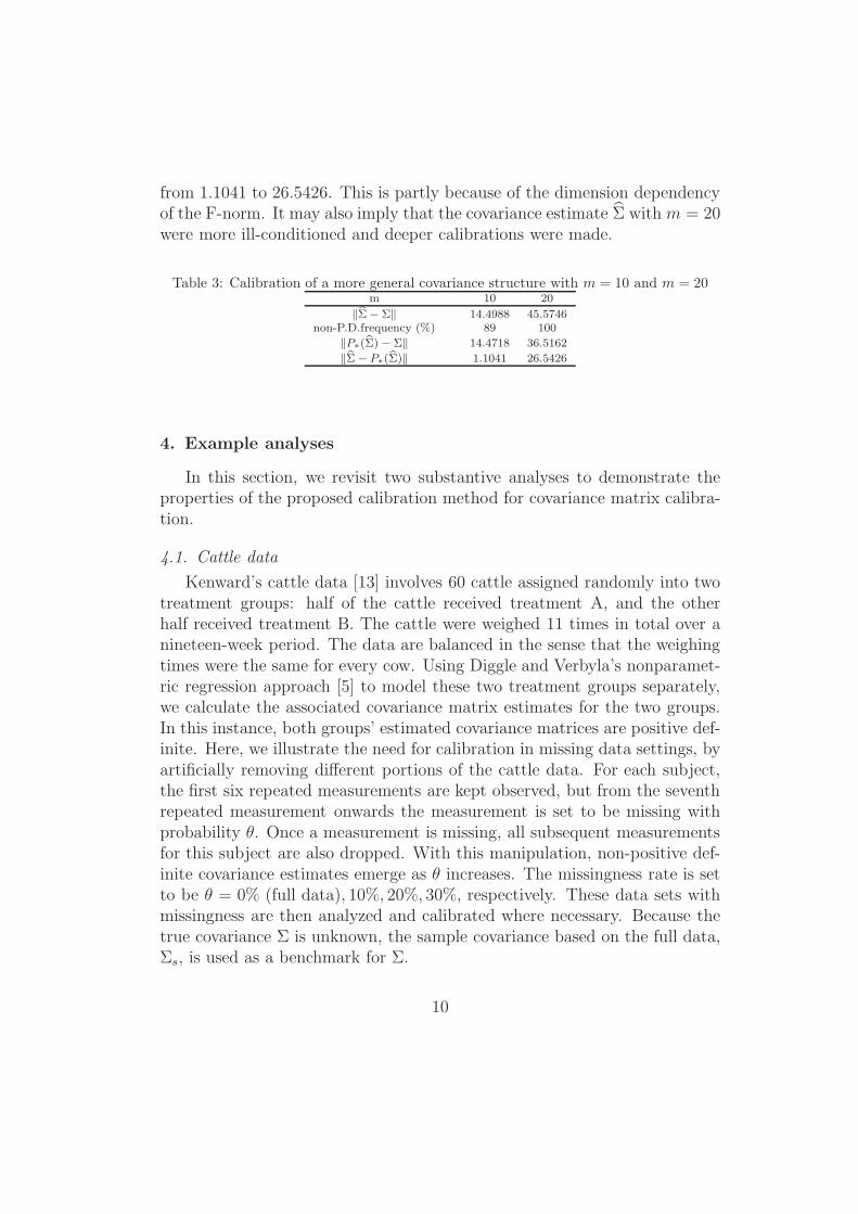
from 1.1041 to 26.5426. This is partly because of the dimension dependencyof the F-norm. It may also imply that the covariance estimate Σ with m = 20were more ill-conditioned and deeper calibrations were made.

Table 3: Calibration of a more general covariance structure with m = 10 and m = 20m 10 20

‖Σ−Σ‖ 14.4988 45.5746non-P.D.frequency (%) 89 100

‖P∗(Σ)− Σ‖ 14.4718 36.5162

‖Σ− P∗(Σ)‖ 1.1041 26.5426

4. Example analyses

In this section, we revisit two substantive analyses to demonstrate theproperties of the proposed calibration method for covariance matrix calibra-tion.

4.1. Cattle data

Kenward’s cattle data [13] involves 60 cattle assigned randomly into twotreatment groups: half of the cattle received treatment A, and the otherhalf received treatment B. The cattle were weighed 11 times in total over anineteen-week period. The data are balanced in the sense that the weighingtimes were the same for every cow. Using Diggle and Verbyla’s nonparamet-ric regression approach [5] to model these two treatment groups separately,we calculate the associated covariance matrix estimates for the two groups.In this instance, both groups’ estimated covariance matrices are positive def-inite. Here, we illustrate the need for calibration in missing data settings, byartificially removing different portions of the cattle data. For each subject,the first six repeated measurements are kept observed, but from the seventhrepeated measurement onwards the measurement is set to be missing withprobability θ. Once a measurement is missing, all subsequent measurementsfor this subject are also dropped. With this manipulation, non-positive def-inite covariance estimates emerge as θ increases. The missingness rate is setto be θ = 0% (full data), 10%, 20%, 30%, respectively. These data sets withmissingness are then analyzed and calibrated where necessary. Because thetrue covariance Σ is unknown, the sample covariance based on the full data,Σs, is used as a benchmark for Σ.

10

Table 4: Calibration results of cattle data with/without missingnessPositive F-Norm among Σ, Σs and P∗(Σ)

θ definiteness of Σ ‖Σ−Σs‖ ‖P∗(Σ)− Σs‖ ‖Σ− P∗(Σ)‖A 0% Yes 116.8018 116.8018 0

10% Yes 197.2300 197.2300 020% No 215.1713 213.5823 12.782130% No 347.9251 344.2363 24.2091

B 0% Yes 109.7911 109.7911 010% Yes 307.9060 307.9060 020% Yes 348.7275 348.7275 030% No 511.1006 498.6707 30.1888

Table 4 shows that for the full data set or cases with relatively low miss-ingness rates (treatment A with missing rate up to 10%, treatment B with

missing rate up to 20%), the Σ are positive definite. In these cases, the

calibrated matrices P∗(Σ) are identical to Σ, the calibration keeping Σ un-changed. When the missing rate increases to 20% for treatment A and 30%for treatment B, Σ become non-positive definite. In these circumstances,the proposed calibration method yields surrogate matrices P∗(Σ) that arepositive-definite and whose Frobenius distances to Σs are shorter than thosefrom Σ.

4.2. CD4+ data

Figure 1: Variograms of CD4+ data

11

The CD4+ data comes from an AIDS cohort study [12] comprising 369infected patients. In total, 2376 repeated measurements of CD4+ cell countswere taken over a period of eight and half years. The data are highly un-balanced, with measurement times varying from subject to subject. Diggleand Verbyla [5] analyzed the CD4+ data using their proposed nonparametriccovariance structure estimation method. Their estimated covariance matrixturns to be non-positive definite, however. We reanalyze the CD4+ data andthen use our proposed calibration method to calibrate the original covariancematrix estimate.

Figure 2: Original covariance estimate Σ (left) and its calibration matrix P∗(Σ)(right) in the CD4+ data

The estimated variogram surface is presented in Figure 1, correspondingto Figure 8 of [5]. The variogram varies for time pairs with equal lags,implying that the underlying longitudinal process for the CD4+ cell countsmay be non-stationary. In Figure 2, we plot the original covariance matrixestimate Σ and its calibrated covariance matrix P∗(Σ), where Σ is found tobe non-positive definite, as mentioned by [5]. From Figure 2 we can see that

Σ and P∗(Σ) are very similar in terms of shape and structure, indicating thatthe calibration approach maintains the major characteristics of the originalcovariance matrix.

12

5. Discussion

We have proposed a calibration approach that provides a positive definitesurrogate for any given non-positive definite matrix. The calibrated covari-ance matrix preserves the major characteristics of the original matrix, whilebeing closer to the true covariance than the original matrix, in the senseof the Frobenius norm. Figure 3 illustrates the idea behind our approach,where the dashed circle represents the domain D0 of all positive semidefi-nite matrices whilst the solid circle is the domain Dc of all positive definitematrices with eigenvalues no smaller than c. Given a positive constant c, anon-positive definite matrix Σ’s nearest positive definite matrix Pc(Σ) will becloser to the true covariance matrix, provided Σ ∈ Dc. We might thereforeexpect that using our positive definite surrogate will improve efficiency andaccuracy in mean estimation.

c

P( )c

Figure 3: Illustration plot on Σ, Σ, Pc(Σ) and c

One potential extension is to replace the domain Dc by a more generalset {A : A − diag(c1, . . . , cn) ≥ 0} where the ci are all positive. However,this extension implies different restrictions imposed on the eigenvalues atdifferent positions, which may be difficult to justify. It also uses the samenumber of parameters as the dimension of the covariance matrix, requiring

13

intensive computational efforts, particularly for high-dimensional data. Wefeel that this particular extension is unlikely to offer substantial benefit.

Our proposed method is not constrained by model assumptions, andhence can be used in both likelihood-based methods (such as generalisedlinear models) and moment-based approaches (such as generalized estimat-ing equations). Neither is it limited by data structures, indicating it can beapplied into any multivariate data setting. In principle, it is applicable toany field of multivariate data analysis where non-positive definiteness of acovariance matrix estimator is a concern. Since the proposed approach is acalibration approach, rather than a covariance estimation approach itself, itcan be directly incorporated in any existing covariance estimation process,and offers a routine check and calibration of covariance matrix estimators.

Appendix: Proof of Theorem 1

We seekPc(X) = argmin

A∈Dc

‖X − A‖.

Rewrite this as

argminA:(A−cI)∈D0

‖(X − cI)− (A− cI)‖ = argminA′∈D0

‖(X − cI)−A′‖+ cI.

From [9], this latter is just P0(X − cI) + cI, as required. If, further, X issymmetric, it has spectral decomposition X = QΛQ⊤ (say) for orthogonal Qand diagonal Λ. Therefore X − cI = Q(Λ− cI)Q⊤, and

Pc(X) = Qdiag{max(λ1 − c, 0), . . . ,max(λn − c, 0)}Q⊤ + cI.

But cI = QcQ⊤, so Pc(X) = Qdiag{max(λ1, c), . . . ,max(λn, c)}Q⊤, as re-quired. �

Acknowledgements

We gratefully acknowledge very constructive comments and suggestions madeby the Editor, AE and one anonymous reviewer, which leads to significantimprovements to the paper.

14

References

[1] Akaike, H. (1974). A new look at the statistical model identification.IEEE Transactions on Automatic Control, 19, 716-723.

[2] Borsdorf, R. and Higham, N.J. (2010). A Preconditioned Newton Al-gorithm for the Nearest Correlation Matrix. IMA Journal of NumericalAnalysis, 30, 94-107.

[3] Chtelat, D. and Wells, M.T. (2016). Improved second order estimationin the singular multivariate normal model. Journal of Multivariate Anal-ysis, 147, 1-19.

[4] Diggle, P. J. (1988). An approach to the analysis of repeated measures.Biometrics, 44, 959-971.

[5] Diggle, P.J. and Verbyla, A. P. (1998). Nonparametric estimation ofcovariance structure in longitudinal data. Biometrics, 54, 401-415.

[6] Fan, J.Q. and Li, R.Z. (2001). Variable Selection via Nonconcave Penal-ized Likelihood and its Oracle Properties. Journal of Royal StatisticalAssociation, 96, 1348-1360.

[7] Halmos, P.R. (1972). Positive approximants of operators. Indiana Univ.of Math. J., 21, 951-960.

[8] Hendrikse, A.J., Spreeuwers, L.J. and Veldhuis, R.N.J. (2009). A Boot-strap Approach to Eigenvalue Correction. Ninth IEEE InternationalConference on Data Mining, 818-823.

[9] Higham, N.J. (1988). Computing a nearest symmetric positive semidef-inite matrix. Linear Algebra and Appl., 103, 103-118.

[10] Higham, N.J. (2008). Functions of Matrices: Theory and ComputationSIAM.

[11] Higham, N.J. The matrix Computation Toolbox. http://www.maths.manchester.ac.uk/~higham/mctoolbox/.

[12] Kaslow, R. A., Ostrow, D. G., Detels, R., et al. (1987). The Multicen-ter AIDS Cohort Study: Rationale, organization and selected charac-teristics of the participants. American Journal of Epidemiology, 126,310-318.

15

[13] Kenward, M.G. (1987). A method for comparing profiles of repeatedmeasurements. A. ppl. Statist., 36, 296-308.

[14] Li, Y. (2011). Efficient semiparametric regression for longitudinal datawith nonparametric covariance estimation. Biometrika, 98(2), 355-370.

[15] Pourahmadi, M. (1999). Joint mean-covariance models with applicationsto longitudinal data: Unconstrained parameterisation. Biometrika, 86,677-90.

[16] Qi, H.D. and Sun, D. (2006). A quadratically convergent Newton methodfor computing the nearest correlation matrix. SIAM J. Matrix Anal.Appl., 28, 360-385.

[17] Rebonato, R. and Jackel P. (2000). The most general methodology tocreate a valid correlation matrix for risk management and option pricingpurposes. J. of Risk, 2, 17-27.

[18] Saleh, A.K.Md.E and Shalabh (2014). A ridge regression estimation ap-proach to the measurement error model. Journal of Multivariate Anal-ysis, 123, 68-84.

[19] Sheena, Y. (2013). Modified estimators of the contribution rates of pop-ulation eigenvalues. Journal of Multivariate Analysis, 115, 301-316.

[20] Srivastava, M.S. and Yanagihara, H. (2010). Testing the equality of sev-eral covariance matrices with fewer observations than the dimension.Journal of Multivariate Analysis, 101(6), 1319-1329.

[21] Tibshirani, R.J. (1996). Regression shrinkage and selection via the lasso.Journal of the Royal Statistical Society , Series B, 58, 267-288.

[22] Wang, Y.G. and Carey, V. (2003). Working correlation structure mis-specification, estimation and covariate design: Implications for general-ized estimating equations performance. Biometrika, 90, 29-41.

[23] Wothke, W. (1993). Nonpositive definite matrices in structural model-ing. In K. A. Bollen, K.A. and Long, J.S. (Editors), Testing structuralequation models. Newbury Park, CA: Sage, 256-293.

[24] Zarowski., Christopher J. (2004). An Introduction to Numerical Analysisfor Electrical and Computer Engineers. Wiley.

16

[25] Zeger, S.L. and Diggle, P.J. (1994). Semiparametric Models for Longi-tudinal Data with Application to CD4 Cell Numbers in HIV Serocon-verters. Biometrics, 50, 689-699.

17