calibration scenarios

8/7/2019 Calibration Scenarios

http://slidepdf.com/reader/full/calibration-scenarios 1/27

Uncertainty Analysis for

Alternative Calibration Scenarios1

Howard Castrup, Ph.D.

PresidentIntegrated Sciences Group

Bakersfield, CA 93306

[email protected]

Suzanne Castrup

Vice President, Engineering

Integrated Sciences GroupBakersfield, CA 93306

[email protected]

AbstractCalibrations are performed to obtain an estimate of the value or bias of selected unit-under-test

(UUT) attributes. In general, calibrations are not considered complete without statements of the

uncertainty in these estimates. Developing these statements requires accounting for all relevantsources of measurement error and assembling these errors in a way that yields viable uncertainty

estimates. Frequently, there is confusion regarding which error sources to include and how to

assemble them. Much of this confusion can be eliminated by both a rigorous examination of theobjective of each UUT attribute calibration and a consideration of the corresponding

measurement configuration or “scenario.”

In this paper, the calibration of a UUT attribute2

is examined within the context of four scenarios.

Each scenario yields a calibration result and a description of measurement process errors thataccompany this result. This information is summarized and then employed to obtain an

uncertainty estimate in the calibration result. The approach taken is one in which the uncertainty

estimate can be applied to estimate measurement decision risk, UUT attribute bias and in-

tolerance probability. Examples are given to illustrate concepts and procedures.

IntroductionThis paper discusses information obtained from measurements made during calibration and the

application of this information to measurement decision risk analysis in the context of four

calibration scenarios:

1. The measurement reference (MTE) measures the value of a passive attribute of the unitunder test (UUT).

2. The UUT measures the value of a passive reference attribute of the MTE.

1 Presented at the NCSLI Workshop & Symposium, Orlando, August 2008.2 An attribute is a measurable characteristic, feature or aspect of an object or substance.



- 2 -

3. The UUT and MTE each provide an “output” or “stimulus” for comparison using a

comparator.

4. The UUT and MTE both measure the value of an attribute of a common artifact that

provides an output or stimulus.

The information obtained includes an observed value, referred to as a “measurement result” or “calibration result,” and an estimated uncertainty in the measurement error. For each scenario, a

measurement equation is given that is applicable to the manner in which calibrations are performed and calibration results are recorded or interpreted.

The measurement scenarios turn out to be simple and intuitive. In each, the measurement result

and the measurement error are separable, allowing the estimation of measurement uncertainty.

For the purposes of this paper, it is assumed in each scenario that the measurement result is anestimate of the value of the bias of the UUT attribute.

Basic Notation

The subscripts and variables designators in this paper are summarized in Table 1.

Table 1. Basic Notation

Notation Description

e an individual measurement process error,such as repeatability, resolution error, etc.

ε combined errors comprised of individualmeasurement process errors

m measurement

b bias

cal calibrationtrue true value

n nominal value

With this notation, for example, measurement error is represented by the quantity ε m, the error in

a calibration result by ε cal and the bias in the UUT attribute is represented by the quantity eUUT ,b.

As stated in the introduction, specific measurement equations will be given for each calibrationscenario. In each equation, quantities relating to the UUT are indicated with the notation x and

quantities relating to the MTE with the notation y. For example, in Scenario 1, where the MTE

directly measures the value of the UUT attribute, the relevant measurement equation is

true m y x ε = + , (1)

where y represents a measurement taken with the MTE, xtrue is the true value of the UUT

attribute and ε m is the measurement error. Variations of Eq. (1) will be encountered throughoutthis paper.



- 3 -

Measurement Uncertainties

Measurement errors and parameter biases are random variables that follow statistical

distributions. Each distribution is a relationship between the value of an error and its probabilityof occurrence. Distributions for errors that are tightly constrained correspond to low uncertainty,

while distributions for errors that are widely spread correspond to high uncertainties.

Mathematically, the uncertainty due to a particular error is equated to the spread in itsdistribution. This spread is just the distribution standard deviation which is defined as the square

root of the distribution variance [1-3]. Letting u represent uncertainty and “var(ε )” the statistical

variance of the distribution of an error ε , we write

var( )u ε = . (2)

This expression will be used in this paper as a template for estimating measurement process

uncertainties encountered in the various calibration scenarios.

Measurement Error Sources

Typically, calibration scenarios feature the following set of measurement process errors or “error

sources.”

eMTE,b = bias in the measurement reference

erep = repeatability or “random” error

eres = resolution error

eop = operator bias

eother = other measurement error, such as that due to environmental corrections, ancillaryequipment variations, response to adjustments, etc.

Measurement Reference Bias

The error in a measurement reference attribute, at any instant in time, is composed of asystematic component and a random component. The systematic component is called “attribute

bias.” Attribute bias is an error component that persists from measurement to measurement

during a “measurement session.” Attribute bias excludes resolution error, random error, operator bias and other sources of error that are not properties of the attribute.

3

Repeatability

Repeatability is a random error that manifests itself as differences in measured value from

measurement to measurement during a measurement session. It should be said that randomvariations in UUT attribute value and random variations due to other causes are not separable

from random variations in the value of the MTE reference attribute or any other error source.

Consequently, whether erep manifests itself in a sample of measurements made by the MTE or bythe UUT, it must be taken to represent a “measurement process error” rather than an error attributable to any specific influence.

3 For purposes of discussion, a measurement session is considered to be an activity in which a measurement or

sample of measurements is taken under fixed conditions, usually for a period of time measured in seconds, minutes

or, at most, hours.



- 4 -

Resolution Error

Reference attributes and/or UUT attributes may provide indications of sensed or stimulated

values with some finite precision.

For example, a voltmeter may indicate values to four, five, six, etc., significant digits. A tape

measure may provide length indications in meters, centimeters and millimeters. A scale mayindicate weight in terms of kg, g, mg, etc. The smallest discernible value indicated in a

measurement comprises the resolution of the measurement.

The basic error model for resolution error is

xindicated = x sensed + eres,

where x sensed is a “measured” value detected by a sensor or provided by a stimulus, xindicated is the

indicated representation of x sensed and eres is the resolution error.

Operator Bias

Because of the potential for operators to acquire measurement information from an individual perspective or to produce a systematic bias in a measurement result, it sometimes happens that

two operators observing the same measurement result will systematically perceive or producedifferent measured values. The systematic error in measurement due to the operator’s

perspective or other tendency is referred to as Operator Bias.

Operator bias is a "quasi-systematic" error, the error source being the perception of a human

operator. While variations in human behavior and response lend this error source a somewhat

random character, there may be tendencies and predilections inherent in a given operator that persist from measurement to measurement.

The random contribution is included in the random error source discussed earlier. Thesystematic contribution is the operator bias.

Repeatability and Resolution Error

It is sometimes argued that repeatability is a manifestation of resolution error. To address this

point, imagine three cases. In the first case, values obtained in a random sample of

measurements take on just two values and the difference between them is equal to the smallestincrement of resolution. If this is the case, we can conclude that “background noise” random

variations are occurring that are beyond the resolution of the measurement. If so, we cannot

include repeatability as an error source but must acknowledge that the apparent randomvariations are due to resolution error. Accordingly, the uncertainty due to resolution error should

be included in the total measurement uncertainty but the uncertainty due to repeatability shouldnot.

In the second case, values obtained in a random sample are seen to vary in magnitude

substantially greater than the smallest increment of resolution. In this case, repeatability cannot

be ignored as an error source. In addition, since each sampled value is subject to resolutionerror, resolution error should also be separately accounted for. Accordingly, the total



- 5 -

measurement uncertainty must include contributions from both repeatability uncertainty and

resolution uncertainty.

The third case is not so easily dealt with. In this case. values obtained in a random sample of

measurements are seen to vary in magnitude somewhat greater than the smallest increment of

resolution but not substantially greater. In this case, we perceive an error due to repeatabilitythat is separable from resolution error but is partly due to it. In this case, it becomes a matter of

opinion as to whether to include repeatability and resolution error in the total measurement error.

Until a clear solution to the problem is found, it is the opinion of the authors that both should beincluded in this case.

Other Error

Other measurement error is a catch-all label applied to errors such as those due to environmentalcorrections, ancillary equipment variations, response to adjustments, etc. For example, suppose

that “other” error is due to an environmental factor, such as temperature, vibration, humidity or

stray emf. In many cases, as in accommodating thermal expansion, the effect of an

environmental factor can be corrected for. Such corrections usually rely on a measurement of the driving environmental factor.

When this happens, the parameter that measures the environmental factor is referred to as an

ancillary parameter. An example would be a thermometer reading used to correct for thermal

expansion in the measurement reference and the UUT attributes. An ancillary parameter issubject to error as is any other parameter, and this error can lead to an error in the environmental

correction. The uncertainty in the error of the correction is a function of the uncertainty in the

error due to the environmental factor.

For a more complete discussion on uncertainties due to environmental and other ancillary

factors, see Ref [1].

Calibration Error and Measurement Error

For the scenarios discussed in this paper, the result of a calibration is taken to be the estimationof the bias eUUT,b of the UUT attribute. The error in the calibration result is represented by the

quantity ε cal . In all scenarios, the uncertainty in the estimation of eUUT,b is computed as the

uncertainty in ε cal . For some scenarios, ε cal is synonymous with the measurement error ε m or its

negative -ε m. In other scenarios, as in Scenario 2 where the UUT measures the MTE attribute, ε m

includes eUUT,b. Since eUUT,b cannot be included in ε cal , the latter of which is the error in the

estimation of eUUT,b, we have a situation where ε cal and ε m may not be of the same sign or

magnitude.

UUT Attribute Bias

For calibrations, it is tacitly assumed that the UUT attribute of interest is assigned some design

or “nominal” value xn. The difference between the UUT attribute’s true value, xtrue, and thenominal value xn is the UUT attribute’s bias eUUT,b. Accordingly, we can write

,true n UUT b x x e= + . (3)



- 6 -

In some cases, the UUT is a passive item, such as a gage block or weight, whose attribute of

interest is a simple characteristic like length or mass. In other cases the UUT is an active device,such as a voltmeter or tape measure, whose attribute consists of a reading or other output, like

voltage or measured length. In the former case, the concepts of true value and nominal value are

straightforward. In the latter case, some comment is needed.

As stated earlier, we consider the result of a calibration to be an estimate the quantity eUUT,b.

From Eq. (3), we can readily appreciate that, if we can assign the UUT a nominal value xn,

estimating xtrue is equivalent to estimating eUUT,b. Additionally, we acknowledge that eUUT,b is an“inherent” property of the UUT, independent of its resolution, repeatability or other

characteristic dependent on its application or usage environment. Accordingly, if the UUT’s

nominal value consists of a measured reading or other actively displayed output, the UUT biasmust be taken to be the difference between the true value of the quantity being measured and the

value internally sensed by the UUT, with appropriate environmental or other adjustments applied

to correct this value to reference (calibration) conditions.

For example, imagine that the UUT is a steel yardstick whose length is a random variablefollowing a statistical distribution with a standard deviation arising from variations in the

manufacturing process. Imagine now that the UUT is used under specified nominalenvironmental conditions. While under these conditions, repeatability, resolution error, operator

bias and other error sources may come into play, the bias of the yardstick is systematically

present, regardless of whatever chance relationship may exist between the length of the measuredobject, the closest observed “tick mark,” the temperature of the measuring environment, the

perspective of the operator, and so on.

MTE Bias

The value of the reference attribute of the MTE, against which the value of the UUT attribute is

compared, has an inherent deviation eMTE,b from its nominal value or a value stated in acalibration certification or other reference document. Letting ytrue represent the true value of the

MTE attribute and letting yn represent the MTE attribute nominal or assumed value, we have

,true n MTE b y y e= + . (4)

In some cases, the MTE is a passive item, such as a gage block or weight, whose attribute is a

simple characteristic like length or mass. In other cases the MTE is an active device, such as a

voltmeter or tape measure, whose attribute consists of a reading or other output, like voltage or measured length. In either case, it is important to bear in mind that eMTE,b is an inherent property

of the MTE, exclusive of other errors such as MTE resolution or the repeatability of the

measurement process. It may vary with environmental deviations, but can usually be adjusted or

corrected to some reference set of conditions. An example of such an adjustment is given inScenario 1 below.

Calibration ScenariosThe four calibration scenarios identified in this paper’s introduction are described in detail in the

following discussions. The descriptions are not offered to serve as recipes to be followed as

dogma but are instead intended to provide guidelines for developing uncertainty estimates

relevant to each scenario. It is hoped that the structure and content of each description will assist



- 7 -

in developing whatever mathematical customization is needed for specific measurement

situations.

In each scenario, we have a measurement of eUUT ,b, denoted δ , and a calibration error ε cal . Thegeneral expression is

,UUT b cal eδ ε = + .

Since eUUT ,b is the quantity being estimated by calibration, as discussed earlier, the uncertainty of

interest is understood to be the uncertainty in δ given the UUT bias eUUT ,b. Then, by Eq. (2), wehave

,

var( )

var( )

var( ) .

cal

UUT b cal

cal

u

e

δ

ε

ε

=

+

=

(5)

UUTUUTUUT

Attribute:

9 VDC

Fixed Value

MTEMTEMTE

Attribute:

DMM Reading

OUTPUT

Figure 1. Scenario 1 – The MTE measures the value of a UUT Attribute.The output is the battery voltage.

Scenario 1: The MTE Measures the UUT Attribute Value

In this scenario, the UUT is a passive device whose calibrated attribute provides no reading or

other metered output. Its output may consist of a generated value, as in the case of a voltage

reference, or a fixed value, as in the case of a gage block.4

The measurement Eq. is repeatedfrom Eq. (1) as

true m y x ε = + , (6)

where y is the measurement result obtained with the MTE, xtrue is the true value of the UUT

attribute and ε m is the measurement error.

The “measured” value provided by the UUT is its nominal value xn, given in Eq. (3), so that

xtrue = xn + eUUT,b. (7)

4 Cases where the MTE measures the value of a metered or other UUT attribute exhibiting a displayed value are

covered later as special instances of Scenario 4.



- 8 -

Substituting Eq. (7) in Eq. (6), we write the measurement equation as

,n UUT b m y x e ε = + + .

The difference y – xn is a measurement of the UUT bias eUUT ,b. We denote this quantity by the

variable δ and write

,

, .

n

UUT b m

UUT b cal

y x

e

e

δ

ε

ε

= −= +

= +

(8)

For this scenario, the calibration error ε cal is equal to the measurement error ε m and is comprisedof MTE bias, measurement process repeatability, MTE resolution error, operator bias, etc. The

appropriate expression is

,cal MTE b rep res op other e e e e eε = + + + + . (9)

Since the UUT is a passive device in this scenario, resolution error, and operator bias arise

exclusively from the use of the MTE, i.e., eUUT ,res and eUUT ,op are zero. In addition, the

uncertainty due to repeatability is estimated from a random sample of measurements taken withthe MTE. Still, variations in UUT attribute value may contribute to this estimate. However,

random variations in UUT attribute value and random variations due to other causes are not

separable from random variations due to the MTE. Consequently, as stated earlier, erep must betaken to represent a “measurement process error” rather than an error attributable to any specific

influence. Given these considerations, the error sources erep, eres and eop in Eq. (9) are

,

,

, ,

rep MTE rep

res MTE res

op MTE op

e e

e e

e e

=

=

=

(10)

where eMTE ,rep represents the repeatability of the measurement process. The “MTE” part of thesubscript indicates that the uncertainty in the error will be estimated from a sample of measurements taken by the MTE.

In some cases, the error source eother may need some additional thought. For example, supposethat eother arises from corrections ensuing from environmental factors, such as thermal expansion.

If measurements are made of the length of a UUT gage block using an MTE reference “super

mike,” it may be desired to correct measured values to those that would be attained at some

reference temperature, such as 20 °C.

Let δ UUT ,env and δ MTE ,env represent thermal expansion corrections to the gage block and super

mike dimensions, respectively. Then the mean value of the measurement sample would becorrected by an amount equal to

5

, ,env MTE env UUT envδ δ δ = − , (11)

5 The form of this expression arises from the fact that thermal expansion of the gage block results in an inflated gage

block length, while thermal expansion of the supermike results in applying additional thimble adjustments to narrow

the gap between the anvil and the spindle, resulting in a deflated measurement reading.



- 9 -

and the error in the corrections would be written

, , .

other env

TE env UUT env

e e

e e

=

= −(12)

From Eqs. (8) and (5), we can write the uncertainty in the calibration result δ as

var( )cal cal u ε = , (13)

where

,

2 2 2 2 2

,

var( ) var( ) var( ) var( ) var( ) var( )

,

cal MTE b rep res op other

MTE b rep res op other

e e e e e

u u u u u

ε = + + + +

= + + + +(14)

and

,

,

, .

rep MTE rep

res MTE res

op MTE op

u u

u u

u u

=

=

=

(15)

For this scenario, no correlations are present between the error sources shown in Eq. (14). Hence

the simple RSS uncertainty combination. This may not be true for correlations within some of the terms, as may be the case when eother = eenv. In this case, we would have

2 2

, , , ,2other MTE env UUT env env MTE env UUT envu u u u u ρ = + − . (16)

If the same temperature measurement device (e.g., thermometer) is used to make both the UUT

and MTE corrections, we would have ρ env = 1, and

2 2

, , , ,

, ,

2

.

other MTE env UUT env MTE env UUT env

MTE env UUT env

u u u u u

u u

= + −

= −(17)

UUTUUTUUT

Attribute:Micrometer

Reading

MTEMTEMTE

Attribute:

Gage Block0.100 cm Nominal

Dimension

OUTPUT

Figure 2. Scenario 2 – The UUT measures the value of an MTE attribute.The output is the gage block dimension.



- 10 -

Scenario 2: The UUT Measures the MTE Attribute Value

In this scenario, the MTE is a passive device whose reference attribute provides no reading or other metered output. Its output may consist of a generated value, as in the case of a voltage

reference, or a fixed value, as in the case of a gage block.6

The measurement equation is a

variation of Eq. (1)

x = ytrue + ε m , (18)

where x is the value measured by the UUT, ytrue is the true value of the MTE attribute being

measured and ε m is the measurement error. Denoting the nominal or indicated value of the MTEas yn, we can write

ytrue = yn + eMTE,b , (19)

where eMTE,b is defined in Eq. (4). Substituting Eq. (19) in Eq. (18) gives

x = yn + eMTE ,b + ε m , (20)

and

,TE b meδ ε = + (21)

where δ is the measurement of the UUT bias, given by

n yδ = − . (22)

For this scenario, the measurement error is given by

,m UUT b rep res op other e e e e eε = + + + + , (23)

where eUUT,b is the UUT bias defined in Eq. (3), erep is the repeatability of the measurement

process as evidenced in the sample of measurements taken with the UUT, eres is the resolution

error of the UUT and eop is operator bias associated with the use of the UUT

,

,

, .

rep UUT rep

res UUT res

op UUT op

e e

e e

e e

=

=

=

(24)

The error source eother may need to include mixed contributions as described in Scenario 1.

Substituting Eq. (23) in Eq. (21) and rearranging gives

, ,UUT b MTE b rep res op other e e e e e eδ = + + + + + (25)

where erep, eres, and eop are defined in Eq. (24).

As before, we obtain an expression that is separable into a measurement δ of the UUT bias,

eUUT,b and an error ε cal given by

,cal MTE b rep res op other e e e e eε = + + + + . (26)

6 Cases where the UUT measures the value of a metered or other MTE attribute exhibiting a displayed value are

covered later as special instances of Scenario 4.



- 11 -

By Eq. (5), the uncertainty in the eUUT ,b estimate in Eq. (25) is

var( )cal cal u ε = , (27)

where2 2 2 2 2

,var( ) .cal MTE b rep res op other u u u u uε = + + + + (28)

Scenario 3: MTE and UUT Output Comparison (Comparator Scenario)

In this scenario, a device called a “comparator” is used to compare UUT and MTE values where

both the UUT and the MTE provide an output value or stimulus. It is worthwhile to consider the

following procedure:

1. The MTE is placed in the comparator.

2. The comparator indication or reading y is noted. This indication or reading is taken to

correspond to the MTE nominal or reading value yn.

3. The MTE is removed and the UUT is placed in the comparator.

4. The comparator indication or reading x is noted.

5. The difference δ is calculated, where

δ = x – y (29)

is taken to be a measurement of the UUT bias eUUT ,b. The UUT corrected value, denoted xc, is

then given by

c n x y δ = + . (30)

UUTUUTUUT

Attribute:

10 gm

Nominal Mass

OUTPUT

MTEMTEMTE

Attribute:

10.000 gm

Nominal Mass

OUTPUT

Figure 3. Scenario 3 – Measured values of the UUT and MTE attributesare compared using a comparator. The outputs are the weights of themasses.

In keeping with the basic notation, the indicated value y can be expressed as

,true MTE m y y ε = + (31)

and the indicated value x can be written

,true UUT m x x ε = + (32)



- 12 -

where ε MTE ,m is the measurement error involved in the use of the comparator to measure the MTE

attribute value and ε UUT ,m is the measurement error involved in the use of the comparator to

measure the UUT attribute value.

By Eq. (4), we can write

,true n MTE b y y e= + (33)and

,true n UUT b x x e= + (34)

Substituting Eq. (33) in Eq. (31) gives

, ,n MTE b MTE m y y e ε = + + (35)

and substituting Eq. (34) in Eq. (32) yields

, ,n UUT b UUT m x x e ε = + + . (36)

Using Eqs. (35) and (36) in Eq. (29), we can write

, , , ,( ) ,n n UUT b MTE b UUT m MTE m

x y

x y e e

δ

ε ε

= −

= − + − + −

so that

, , , ,( ) ( )UUT b n n MTE b UUT m MTE me x y eδ ε ε = − − + − − . (37)

In most calibrations involving comparators xn = yn and Eq. (37) becomes7

, , , ,( )UUT b MTE b UUT m MTE me eδ ε ε = + − − . (38)

Then, as with other scenarios, we have by Eq. (38), a measured deviation δ and a calibration

process error ε cal :

, , , ,

,

( )

,

UUT b MTE b UUT m MTE m

UUT b cal

e e

e

δ ε ε

ε

= − + −

= +(39)

where

, , ,( )cal UUT m MTE m MTE beε ε ε = − − . (40)

Letting ec,b represent the bias of the comparator, ε MTE ,m is given by8

7 To accommodate cases where yn ≠ xn, δ is redefined as

δ = ( x – xn) – ( y – yn) .

As an example where xn ≠ yn, consider a case where the MTE is a 2 cm gage block and the UUT is a 1 cm gage block. Suppose that the comparator readings for the MTE and UUT are 2.10 cm and 0.99 cm, respectively. Then

δ = (0.99 − 1.0 ) – (2.10 − 2.0) = − 0.110 cm ,

and, using Eq. (30), we have

xc = 2.0 cm + (0.99 - 2.10 ) cm = (2.0 – 1.11) cm = 0.89 cm.



- 13 -

, , , , , ,TE m c b MTE rep MTE res MTE op MTE other e e e e eε = + + + + . (41)

and ε UUT ,m is

, , , , , ,UUT m c b UUT rep UUT res UUT op UUT other e e e e eε = + + + + . (42)

By Eqs. (39) and (5), the measurement uncertainty in δ is obtained from

var( )cal cal u ε = ,

where

2 2 2 2 2

,var( )cal MTE b rep res op other u u u u uε = + + + + . (43)

In this scenario,

2

, ,

2 2 2

, , , ,

2 2 2

, , , ,

2 2 2

, , , , , ,

var( )

var( )

var( )

var( ) 2

MTE b MTE b

rep UUT rep MTE rep MTE rep UUT rep

res UUT res MTE res MTE res UUT res

op UUT op MTE op MTE op UUT op op MTE op UUT op

u e

u e e u u

u e e u u

u e e u u u u ρ

= −

= − = +

= − = +

= − = + −

(44)

and2 2 2

, , , , , ,var( ) 2other UUT other MTE other MTE other UUT other other MTE other UUT other u e e u u u u ρ = − = + − , (45)

where ρ other represents the correlation, if any, between eMTE ,other and eUUT ,other .

Scenario 4: The MTE and UUT Measure a Common Artifact

In this scenario, both the MTE and UUT measure the value of a common artifact, where theartifact provides an output or stimulus. The measurements are made and recorded separately.

An example of this scenario is the calibration of a thermometer (UUT) using a temperaturereference (MTE), where both the thermometer and the temperature reference are placed in anoven and the temperatures measured by each are recorded.

We let T denote the true value of the artifact and write the measurement equation as

,UUT m x T ε = + , (46)

and

,TE m y T ε = + , (47)

8 In many comparator calibrations, the comparator device is made up of two measurement arms and a meter or other

indicator. The UUT and the MTE are placed in different arms of the comparator and the difference between the

values is displayed by the indicating device. In such cases, if the UUT and MTE swap locations, and the average of the differences is recorded, then bias cancellation is achieved as in Eq. (43). Of course, the Eqs. (41) and (42) would

need to be modified to accommodate any additional measurement process errors, such as additional contributions

due to comparator resolution error.

If this swapping procedure is not followed, the comparator bias is not cancelled and the applicable scenario becomesa variation of Scenario 1 or 2 in which the comparator, taken in aggregate, is treated as the MTE, with the reference

item, indicating device, comparator arms, etc. acting as components. The estimation of the bias uncertainty of the

aggregate MTE is the subject of multivariate uncertainty analysis, described in Annex 3.



- 14 -

where ε UUT ,m is the measurement process error for the UUT measurement of the artifact’s value

and ε MTE ,m is the measurement process error for the MTE measurement of same.

UUTUUTUUT

Attribute:

Temperature

Reading

MTEMTEMTE

Attribute:

Temperature

Reading

OUTPUT OUTPUT

Figure 4. Scenario 4 – The UUT and the MTE measure a common artifact.The output is the temperature of an oven.

These errors are given by

, , , , , ,UUT m UUT b UUT rep UUT res UUT op UUT other e e e e eε = + + + + (48)

and

, , , , , ,TE m MTE b MTE rep MTE res MTE op MTE other e e e e eε = + + + + . (49)

Substituting these expressions in Eqs. (46) and (47) gives

, , , , ,UUT b UUT rep UUT res UUT op UUT other x T e e e e e= + + + + + (50)

and

, , , , ,TE b MTE rep MTE res MTE op MTE other y T e e e e e= + + + + + . (51)

Defining

yδ = − , (52)

these expressions yield

,UUT b cal eδ ε = + . (53)

where

, , , ,

, , , , ,

( ) ( )

( ) ( ) .

cal UUT rep MTE rep UUT res MTE res

UUT op MTE op UUT other MTE other MTE b

e e e e

e e e e e

ε = − + −

+ − + − −(54)

By Eq. (5), the measurement uncertainty is again given by

var( )cal cal u ε = , (55)where

2 2 2 2 2

,var( ) ,cal MTE b rep res op other u u u u uε = + + + + (56)

and



- 15 -

2

, ,

2 2 2

, , , ,

2 2 2

, , , ,

2 2 2

, , , , , ,

var( )

var( )

var( )

var( ) 2 ,

MTE b MTE b

rep UUT rep MTE rep UUT rep MTE rep

res UUT res MTE res UUT res MTE res

op UUT op MTE op UUT op MTE op op UUT op MTE op

u e

u e e u u

u e e u u

u e e u u u u ρ

= −

= − = +

= − = +

= − = + −

(57)

and2 2 2

, , , , , ,var( ) 2other UUT other MTE other UUT other MTE other other UUT other MTE other u e e u u u u ρ = − = + − , (58)

where, again, ρ other represents a correlation between eMTE ,other and eUUT ,other .

Scenario 4 Special Cases

There are two special cases of Scenario 4 that may be thought of as variations of Scenarios 1 and

2. Both cases are accommodated by the Scenario 4 definitions and expressions developed above.

Case 1: The MTE measures the UUT and both the MTE and UUT provide a metered or other

displayed output.In this case, the common artifact is the UUT attribute, consisting of a “stimulus” embedded in

the UUT. An example would be a UUT voltage source whose output is indicated by a digitaldisplay and is measured using an MTE voltmeter.

Case 2: The UUT measures the MTE and both the MTE and UUT provide a metered or other displayed output.

In this case, the common artifact is the MTE attribute, consisting of a “stimulus” embedded in

the MTE. An example would be an MTE voltage source whose output is indicated by a digital

display and is measured using a UUT voltmeter.

Uncertainty Analysis ExamplesFour scenarios have been discussed that yield expressions for calibration uncertainty that are

useful for risk analysis. In all scenarios and cases, the calibration result is expressed as

,UUT b cal eδ ε = + ,

and the calibration uncertainty is given by

var( )cal cal u ε = .

Examples illustrating the application of the four calibration scenarios to uncertainty analysis are provided below.

Scenario 1: The MTE Measures the UUT Attribute Value

In this scenario, the measurement result is δ = y – xn and ε cal is expressed in Eq. (9). Theexample for this scenario consists of calibrating a 30 gm mass with a precision balance. Local

gravity is considered to be constant during the measurement process. Multiple measurements of the UUT mass are taken and the sample statistics are computed to be

Sample Mean = 30.000047 gm



- 16 -

Standard Deviation = 1.15 × 10-5

gm

Uncertainty in the Mean = 6.64 × 10-6

gmSample Size = 3

The measurement result is δ = (30.000047 – 30) gm = 4.7 × 10-5 gm. However, the

measurements are not taken in a vacuum, so the buoyancy of displaced air can introducemeasurement error. The balance is calibrated with calibration weights with density of 8.0 gm/cm

3. The air buoyancy correction is

( )( )

1 / 8.0

1 /

air

corr

air UUT

y yρ

ρ ρ

−= ×

−

where y is the sample mean, ρ air is the local air density and ρ UUT is the density of the UUT

mass. For this analysis, we will assume that ρ air = 1.2 × 10-3

gm/cm3

and ρ UUT = 8.4 gm/cm3.

The corrected sample mean is computed to be

( )( )

( )( )

1 0.0012 /8.0 1 0.00015

30.000047gm 30.000047gm1 0.0012 /8.4 1 0.00014

0.9998530.000047gm 30.000047gm 0.99999

0.99986

29.99975gm

corr y

− −= × = ×− −

= × = ×

=

and the corrected calibration result is corr δ = (29.99975 – 30) gm = – 2.5 × 10-4

gm.

In the mass calibration scenario, we must account for the following measurement process errors:

• Bias in the precision balance, eMTE,b.

• Repeatability, eMTE,rep.• Error due to the digital resolution of the balance, eMTE,res.• Environmental factors error resulting from the buoyancy correction, eenv.

The error in corr δ is

, , ,cal MTE b MTE rep MTE res enve e e eε = + + +

where

,

1 2air UUT

env UUT enve e

c e c e ρ ρ

=

= +

and air e ρ and UUT e ρ are the errors in the air and UUT densities, respectively. The coefficients c1 and c2 are sensitivity coefficients that determine the relative contribution of the errors

air e ρ and

UUT e ρ to the total error eenv. The sensitivity coefficients are defined below.

9

9 Guidance on the development of multivariate error models is provided in NCSLI RP-12-2008.



- 17 -

( )

( )

1

3 3

3 3

1 / 8.0 1

1 / 1 / 8.0

30.000047gm 1 0.0012 / 8.0 1

1 0.0012 / 8.4 8.4gm/cm 1 0.0012 / 8.4 8.0gm/cm

30.000047gm0.11905cm / gm 0.125 cm / gm

0.99986

30.0042 gm

corr air

air air UUT UUT air UUT

y yc

ρ

ρ ρ ρ ρ ρ ρ

⎡ ⎤∂ −= = × −⎢ ⎥∂ − −⎣ ⎦

⎡ ⎤−= × −⎢ ⎥− × −⎣ ⎦

⎡ ⎤= × −⎣ ⎦

= ( )3 30.0060 cm / gm 0.1785cm× − = −

( )

( ) ( )

2 22

3

2 2

3 4 3

1 /8.0

1 /

0.0012 1 0.0012 /8.030.000047gm cm / gm

8.4 1 0.0012 /8.4

0.9998530.000047gm 0.000017cm / gm 5.1 10 cm

0.99971

corr air air

UUT UUT air UUT

yc y

ρ ρ

ρ ρ ρ ρ

−

∂ −= = − × ×

∂ −

−= − × ×

−

= − × × = − ×

The uncertainty in corr δ is

, , , 1 2

2 2 2 2 2 2 2

, , , 1 2 1 2 , ,

var( )

var( ) var( ) var( ) var( )

2 .

air UUT

air UUT

cal cal

MTE b MTE rep MTE res

MTE b MTE rep MTE res env MTE env UUT env

u

e e e c e c e

u u u c u c u c c u u

ρ ρ

ρ ρ

ε

ρ

=

= + + + +

= + + + + +

The correlation coefficient ρ env accounts for any correlation betweenair

e ρ andUUT

e ρ . The

correlation coefficient can range in value from – 1 to +1. In this analysis, the error in the air density is considered to be uncorrelated to the error in the density of the UUT mass. Therefore,

ρ env = 0 and the uncertainty ucal can be expressed as

( ) ( )

2 2 2 2 2 2 2

, , , 1 2

2 22 2 2

, , , 1 2

air UUT

air UUT

cal MTE b MTE rep MTE res

MTE b MTE rep MTE res

u u u u c u c u

u u u c u c u

ρ ρ

ρ ρ

= + + + +

= + + + +

The distributions, limits, confidence levels and standard uncertainties for each error source aresummarized in Table 2.



- 18 -

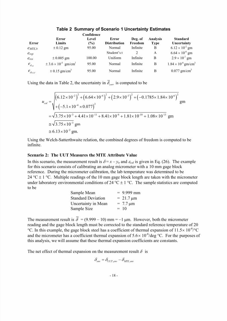
Table 2 Summary of Scenario 1 Uncertainty Estimates

Error

Error

Limits

Confidence

Level

(%)

Error

Distribution

Deg. of

Freedom

Analysis

Type

Standard

Uncertainty

eMTE,b ± 0.12 gm 95.00 Normal Infinite B 6.12 × 10-2 gm

erep Student’s t 2 A 6.64 × 10-6 gm

eres ± 0.005 gm 100.00 Uniform Infinite B 2.9 × 10-3 gm

air e ρ ± 3.6 × 10-5 gm/cm3 95.00 Normal Infinite B 1.84 × 10-6 gm/cm3

UUT e ρ ± 0.15 gm/cm

3 95.00 Normal Infinite B 0.077 gm/cm3

Using the data in Table 2, the uncertainty in corr δ is computed to be

( ) ( ) ( ) ( )

( )

2 2 2 22 6 3 6

24

3 11 6 10 13

3

2

6.12 10 6.64 10 2.9 10 0.1785 1.84 10gm

5.1 10 0.077

3.75 10 4.41 10 8.41 10 1.81 10 1.08 10 gm

3.75 10 gm

6.13 10 gm.

cal u

− − − −

−

− − − − −

−

−

× + × + × + − × ×=

+ − × ×

= × + × + × + × + ×

≅ ×

≅ ×

Using the Welch-Satterthwaite relation, the combined degrees of freedom is computed to beinfinite.

Scenario 2: The UUT Measures the MTE Attribute Value

In this scenario, the measurement result is δ = x – yn and ε cal is given in Eq. (26). The example

for this scenario consists of calibrating an analog micrometer with a 10 mm gage block reference. During the micrometer calibration, the lab temperature was determined to be

24 °C ± 1 °C. Multiple readings of the 10 mm gage block length are taken with the micrometer

under laboratory environmental conditions of 24 °C ± 1 °C. The sample statistics are computedto be

Sample Mean = 9.999 mm

Standard Deviation = 21.7 µm

Uncertainty in Mean = 7.7 µmSample Size = 10

The measurement result is δ = (9.999 – 10) mm = –1 µm. However, both the micrometer

reading and the gage block length must be corrected to the standard reference temperature of 20°C. In this example, the gage block steel has a coefficient of thermal expansion of 11.5 × 10

-6/°C

and the micrometer has a coefficient thermal expansion of 5.6 × 10-6

/deg °C. For the purposes of this analysis, we will assume that these thermal expansion coefficients are constants.

The net effect of thermal expansion on the measurement result δ is

, ,env UUT env MTE envδ δ δ = −



- 19 -

where ,UUT envδ and ,TE envδ represent thermal expansion of the micrometer and gage block

dimensions, respectively. The net length expansion is computed from the temperature difference

∆T , the average measured length x , the coefficient of thermal expansion for the gage block α MTE

and the coefficient of thermal expansion for the micrometer α UUT .

( )

( ) 6

4

4 C 9.999 mm 5.6 11.5 10 / C

= 2.36 10 mm = 0.236µm

env UUT MTE T xδ α α

−

−

= ∆ × × −

= ° × × − × °

− × −

The corrected calibration result corr δ is computed to be

( )1 0.236 µm

= 1.24µm

corr envδ δ δ = +

= − +

−

In the micrometer calibration scenario, we must account for the following measurement process

errors:

• Bias in the value of the 10 mm gage block length, eMTE,b.• Error associated with the repeat measurements taken, eUUT,rep.

• Error associated with the analog resolution of the micrometer, eUUT,res.

• Operator bias resulting from his/her perception of the analog readings, eUUT,op.• Environmental factors error resulting from the thermal expansion correction, eenv.

The error in corr δ is

, , , ,cal MTE b UUT rep UUT res UUT op enve e e e eε = + + + +

where

, ,env UUT env MTE enve e e= −

and eUUT,env and eMTE,env are the errors in the micrometer and gage block length corrections,

respectively.




- 20 -

( ) ( ) ( ) ( ) ( )

( ) ( ) ( ) ( ) ( ) ( )

( ) ( )

, , , , , ,

, , , , , ,

, ,

2 2

, ,

var( )

var var var var var

var var var var var var

2 var var

cal cal

MTE b UUT rep UUT res UUT op UUT env MTE env

TE b UUT rep UUT res UUT op UUT env MTE env

env UUT env MTE env

MTE b UUT rep UUT

u

e e e e e e

e e e e e e

e e

u u u

ε

ρ

=

= + + + + −

+ + + + +=

−

= + + 2 2 2 2

, , , , , ,2 .res UUT op UUT env MTE env env UUT env MTE envu u u u u ρ + + + −

The correlation coefficient ρ env accounts for any correlation between the environmental

correction errors. In this analysis, both the micrometer and gage block length expansioncorrections will err in the same direction and by a constant proportional amount. Therefore, a

correlation coefficient of +1 should apply and the uncertainty ucal can be expressed as

( )

2 2 2 2 2 2

, , , , , , , ,

22 2 2 2

, , , , , ,

2

.

cal MTE b UUT rep UUT res UUT op UUT env MTE env UUT env MTE env

MTE b UUT rep UUT res UUT op UUT env MTE env

u u u u u u u u u

u u u u u u

= + + + + + −

= + + + + −

The distributions, limits, confidence levels and standard uncertainties for each error source are

summarized in Table 3.


Error

Error Limits

(µm)

Confidence

Level

(%)

Error

Distribution

Degrees of

Freedom

Analysis

Type

Standard

Uncertainty

(µm)

erep Student’s t 9 A 7.7

eres ± 5.0 95.00 Normal Infinite B 2.6

eop ± 5.0 95.00 Normal Infinite B 2.6

eUUT,env ± 0.056 95.00 Normal Infinite B 0.029

eMTE,env ± 0.115 95.00 Normal Infinite B 0.059

eMTE,b + 0.18, -0.13 90.00 Lognormal Infinite B 0.09

Using the data in Table 3, the uncertainty in corr δ is

( ) ( ) ( ) ( ) ( )2 2 2 2 2

7.7 2.6 2.6 0.029 0.056 0.09 µm

59.29 6.76 6.76 0.007 0.0081 µm

72.82 µm

8.53µm

cal u = + + + − +

= + + + +

=

=

Using the Welch-Satterthwaite relation, the combined degrees of freedom is computed to be 14.

Scenario 3: MTE and UUT Attribute Values are Compared

In this scenario, the measurement result is δ = x – y and ε cal is expressed in Eq. (40). Theexample for this scenario consists of calibrating an end gauge, with a nominal length of 50 mm,



- 21 -

using an end gauge standard of the same nominal length. The calibration process consists of

measuring and recording the difference between the two end gauges using a comparator apparatus.

In this case, we are measuring the difference in the lengths of the two end gauges. The sample

statistics are computed to be

Sample Mean = 215 nm

Standard Deviation = 9.7 nmUncertainty in Mean = 4.33 nm

Sample Size = 5

and the measurement result is 215nmδ = . The temperature for both gage blocks during

calibration is 19.9 °C ± 0.5 °C. Consequently, the calibration result must be corrected to the

standard reference temperature of 20 °C. The corrected calibration result corr δ is computed from

, ,

corr env

UUT env MTE env

δ δ δ

δ δ δ = += + −

where

,UUT env UUT T xδ α = ∆ × × = thermal expansion of the UUT end gage

,TE env MTE T yδ α = ∆ × × = thermal expansion of the MTE end gage

δ = y− , the average difference between UUT and MTE end gage

lengths during calibration

α UUT = coefficient of thermal expansion for the UUT end gauge

α MTE = coefficient of thermal expansion for the MTE end gauge∆T = difference in the temperature of the end gauge from the 20 °C

For the purposes of this example, we will assume that α UUT = α MTE = α = 11.5 × 10-6

/°C.

Therefore, corr δ can be expressed as

( )

( )1

corr T x y

T

T

δ δ α

δ α δ

δ α

= + ∆ −

= + ∆

= + ∆

and is computed to be

( )

( )

-6

-6

215nm 1+0.1 C 11.5 10 / C

215nm 1+1.15 10

215nm,

corr δ = ° × × °

= ×

≅

and the corrected value for this example is



- 22 -

(1 )

50 mm + 215 µm

50.0002 mm.

c n corr

n

x y

y T

δ

δ α

= +

= + +

=

≅

The error in the estimate of xc includes the following measurement process errors:

• Bias in the value of the 50 mm end gage standard length, eMTE,b.

• Bias of the comparator, ec,b

• Error associated with the repeat measurements taken, erep.• Digital Resolution error for the comparator, eres.

• Environmental factors error resulting from the thermal expansion correction, eenv.

The combined calibration error in corr δ is, by Eq. (40),

, , ,( )cal UUT m MTE m MTE beε ε ε = − −

where, by Eqs. (41) and (42),

, , , , ,TE m c b MTE rep MTE res MTE enve e e eε = + + +

and

, , , , ,UUT m c b UUT rep UUT res UUT enve e e eε = + + +

where ec,b represents the bias of the comparator. Writing the expression for ecal as

,cal rep res env MTE be e e eε = + + −

we have

, , ,rep UUT rep MTE rep repe e e eδ = − =

, ,res UUT res MTE rese e e= −

, , ,env UUT env MTE env enve e e e

δ = − =

where

1 2,.T env

e c e c eα δ ∆= +

The sensitivity coefficients c1 and c2 are given by

1

6

3

11.5 10 / C 215nm

= 2.47 10 nm / C

env

c T

δ αδ

−

−

∂= =∂∆= × ° ×

× °

and

2

0.1 C 215nm

= 21.5 C-nm

envc T δ

δ α

∂= = ∆∂= ° ×

°




- 23 -

( ) ( ) ( ) ( ), , 1 2 ,,

2 2 2 2 2 2 2 2

, , , , 1 2 ,,

var( )

var var var var

2 .

cal cal

UUT res MTE res T MTE brep

UUT res MTE res res UUT res MTE res T MTE brep

u

e e e c e c e e

u u u u u c u c u u

α δ

α δ

ε

ρ

∆

∆

=

= + − + + + −

= + + − + + +

The resolution uncertainty for the UUT and MTE are equal to the resolution uncertainty of the

comparator, uUUT,res = uMTE,res = uc,res. In addition, the resolution error for the UUT and MTE are

uncorrelated, so that ρ res = 0. Therefore, the uncertainty ucal can be expressed as

2 2 2 2 2 2 2

, 1 2 ,,2cal c res T MTE brep

u u u c u c u uα δ ∆= + + + + .




Error Error Limits

Confidence

Level(%)

ErrorDistribution

Degrees of Freedom

AnalysisType

Standard

Uncertainty(nm)

,repe

δ Student’s t 5 A 4.33 µm

ec,res ± 1 nm 100.0 Uniform Infinite B 0.577 µm

e∆T ± 0.5 °C 95.00 Normal Infinite B 0.255 °C

eα ± 0.5 × 10-6 /°C 95.00 Normal Infinite B ± 0.255 × 10-6 /°C

eMTE,b Student’s t 18 B 25 µm

Using the data in Table 4, the uncertainty in corr δ is

( ) ( ) ( )2 2 23 2 6 2

7 5

4.33 2 0.577 (2.47 10 0.255) (21.5 0.255 10 ) 25 nm

18.75 0.67 3.97 10 3.01 10 625µm

644.4µm

25.4µm.

cal u − −

− −

= + × + × × + × × +

= + + × + × +

=

=


Scenario 4: The MTE and UUT Measure a Common Artifact

For this scenario, both the MTE and UUT measure the value or output of a common artifact.

The measurement result is δ = x – y and ε cal is given in Eq. (54).

The example for this scenario consists of calibrating a digital thermometer at 100 °C using anoven and analog temperature reference. The oven temperature is adjusted using its internal

temperature probe and the readings from the thermometer and temperature reference are

recorded. This process is repeated several times and the resulting sample statistics are computedto be



- 24 -

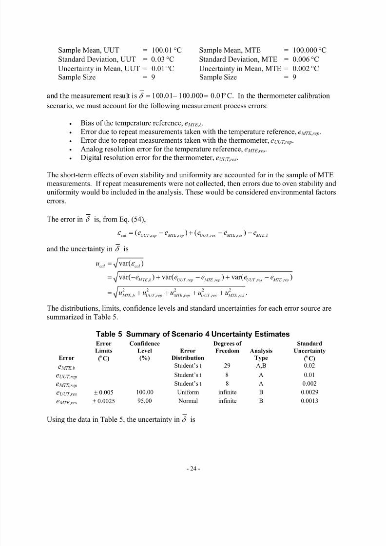
Sample Mean, UUT = 100.01 °C Sample Mean, MTE = 100.000 °C

Standard Deviation, UUT = 0.03 °C Standard Deviation, MTE = 0.006 °C

Uncertainty in Mean, UUT = 0.01 °C Uncertainty in Mean, MTE = 0.002 °CSample Size = 9 Sample Size = 9

and the measurement result is 100.01 100.000 0.01 Cδ = − = ° . In the thermometer calibrationscenario, we must account for the following measurement process errors:

• Bias of the temperature reference, eMTE ,b.

• Error due to repeat measurements taken with the temperature reference, eMTE ,rep.

• Error due to repeat measurements taken with the thermometer, eUUT ,rep.• Analog resolution error for the temperature reference, eMTE ,res.• Digital resolution error for the thermometer, eUUT ,res.

The short-term effects of oven stability and uniformity are accounted for in the sample of MTEmeasurements. If repeat measurements were not collected, then errors due to oven stability and

uniformity would be included in the analysis. These would be considered environmental factorserrors.

The error in δ is, from Eq. (54),

, , , , ,( ) ( )cal UUT rep MTE rep UUT res MTE res MTE be e e e eε = − + − −

and the uncertainty in δ is

, , , , ,

2 2 2 2 2

, , , , ,

var( )

var( ) var( ) var( )

.

cal cal

TE b UUT rep MTE rep UUT res MTE res

MTE b UUT rep MTE rep UUT res MTE res

u

e e e e e

u u u u u

ε =

= − + − + −

= + + + +




Error

Error

Limits

(°C)

Confidence

Level

(%)

Error

Distribution

Degrees of

Freedom Analysis

Type

Standard

Uncertainty

(°C)

eMTE,b Student’s t 29 A,B 0.02

eUUT ,rep Student’s t 8 A 0.01

eMTE ,rep Student’s t 8 A 0.002

eUUT ,res ± 0.005 100.00 Uniform infinite B 0.0029

eMTE ,res ± 0.0025 95.00 Normal infinite B 0.0013

Using the data in Table 5, the uncertainty in δ is



- 25 -

( ) ( ) ( ) ( ) ( )2 2 2 2 2

0.02 0.01 0.002 0.0029 0.0013 C

0.0004 0.0001 0.000004 0.000008 0.000002 C

0.000514 C

0.023 C

cal u = + + + + °

= + + + + °

= °

= °


Measurement Decision Risk Analysis

In each of the scenarios described in this paper, a UUT bias eUUT,b, a measurement of this bias δ ,and a measurement uncertainty ucal have been described. In calibrating a UUT to determine if it

is in- or out-of-tolerance, we face two principal varieties of measurement decision risk; namely,

False Accept Risk and False Reject Risk. The former can be expressed in two ways. First, there

is the probability that a UUT attribute is both out-of-tolerance and observed to be in-tolerance.Second, there is the probability that a UUT attribute, accepted as being in-tolerance, will be out-

of-tolerance. The first alternative is called “unconditional false accept risk” or UFAR. Thesecond is called “conditional false accept risk” or CFAR.

10

False reject risk ( FRR) is the probability that a UUT attribute will be both in-tolerance and

perceived as being out-of-tolerance.11

UFAR, CFAR and FRR are computed for each of the scenarios presented in this paper in a

companion article titled “Decision Risk Analysis for Alternative Calibration Scenarios” [9].

10 UFAR and CFAR are also referred to respectively as the “probability of a false accept” or PFA and the

“conditional probability of a false accept” or CPFA. In much of the literature, UFAR is also referred to as

“Consumer’s Risk.”11 False reject risk is sometimes called the “probability of a false reject” or PFR.



- 26 -

Nomenclature Nomenclature used in this paper for the principal quantities is summarized in Table 6. The

notation for other quantities can be determined by applying the notation of Table 1.

Table 6. NomenclatureQuantity Description

UUT Unit Under Test. The artifact undergoing calibration.

Attribute A measurable property of a device, substance or other quantity.

MTE Measuring or Test Equipment. The measurement reference.

ε m The total error in the measurement of the value of an attribute.

eUUT ,b (1) The bias of a UUT attribute as received for calibration. (2)The quantity estimated by UUT calibration.

uUUT ,b The uncertainty in the bias of a UUT attribute as received for calibration. Equal to the standard deviation of the eUUT ,b

distribution.eMTE ,b The bias of the MTE attribute used to calibrate the UUT

attribute.

ε UUT ,m The error in measurements made with the UUT attribute or theerror in measuring the UUT attribute’s value with a comparator.

ε MTE ,m The error in measurements made with the MTE attribute or theerror in measuring the MTE attribute’s value with a comparator.

δ The result of a UUT calibration, i.e., an estimate of eUUT ,b obtained by calibration.

ε cal The error in δ .

ucal The uncertainty in ε cal . xn The nominal value of a UUT attribute.

xtrue The true value of a UUT attribute.

yn The nominal value of an MTE attribute.

ytrue The true value of an MTE attribute.

xc The value of the UUT attribute indicated by a measurementtaken with a comparator.

ec,b The bias in a comparator indication.

UFAR Unconditional False Accept Risk. The probability that an out-

of-tolerance UUT attribute will be observed to be in-tolerance.

CFAR Conditional False Accept Risk. The probability that an acceptedUUT attribute will be out-of-tolerance.

FRR False Reject Risk. The probability that an in-tolerance UUTattribute will be observed to be out-of-tolerance.



AcknowledgmentsThe authors are indebted to Dr. Dennis Jackson, Mr. Del Caldwell, Mr. Jerry Hayes and Mr.

Scott Mimbs for valuable suggestions which helped to clarify the descriptions of the four calibration scenarios presented in the paper. We would also like to especially thank Mr.

Caldwell for his thorough review of and insightful comments on much of the preliminary work

leading up to this publication.

References[1] NCSLI, Determining and Reporting Measurement Uncertainties, Recommended Practice

RP-12, NCSL International, Under Revision.

[2] NASA, Measurement Uncertainty Analysis Principles and Methods, KSC-UG-2809,

National Aeronautics and Space Administration, November 2007.

[3] ISG, Analytical Metrology Handbook , Integrated Sciences Group,

www.isgmax.com/analytical_metrology.htm, 2006.

[4] Castrup, H., “Risk Analysis Methods for Complying with Z540.3,” Proc. NCSLI Workshop& Symposium, St. Paul, 2007.

[5] ISG, RiskGuard 2.0, www.isgmax.com/risk_freeware.htm, © 2007, Integrated Sciences

Group.

[6] ISG, UncertaintyAnalyzer 3.0, www.isgmax.com/unc_features.htm, © 2005-2006 IntegratedSciences Group.

[7] ISG, Uncertainty Sidekick Pro, www.isgmax.com/sidekickpro_features.htm, © 2006-2007,

Integrated Sciences Group.

[8] ISG, Uncertainty Sidekick, www.isgmax.com/uncertainty_freeware.htm, © 2005-2007,

Integrated Sciences Group.

[9] Castrup, H., “Decision Risk Analysis for Alternative Calibration Scenarios,” Presented at the

NCSLI Workshop & Symposium, Orlando, 2008.

calibration scenarios

Documents