Calibration/Optimisation

Dr Andy Evans

Preparing to model

Verification

Calibration/OptimisationValidationSensitivity testing and dealing with error

ParametersIdeally we’d have rules that determined behaviour:

If AGENT in CROWD move AWAY

But in most of these situations, we need numbers:if DENSITY > 0.9 move 2 SQUARES NORTH

Indeed, in some cases, we’ll always need numbers:if COST < 9000 and MONEY > 10000 buy CAR

Some you can get from data, some you can guess at, some you can’t.

Calibration

Models rarely work perfectly.Aggregate representations of individual objects.Missing model elementsError in data

If we want the model to match reality, we may need to adjust variables/model parameters to improve fit.This process is calibration.

First we need to decide how we want to get to a realistic picture.

Model runsInitialisation: do you want your model to:

evolve to a current situation?

start at the current situation and stay there?

What data should it be started with?

You then run it to some condition:some length of time?some closeness to reality?

Compare it with reality.

Calibration methodologies

If you need to pick better parameters, this is tricky. What combination of values best model reality?

Using expert knowledge.Can be helpful, but experts often don’t understand the inter-relationships between variables well.

Experimenting is lots of different values.Rarely possible with more than two or three variables because of the combinatoric solution space that must be explored.

Deriving them from data automatically.

Processing

Models vary greatly in the processing they require.

a) Individual level model of 273 burglars searching 30000 houses in Leeds over 30 days takes 20hrs.

b) Aphid migration model of 750,000 aphids takes 12 days to run them out of a 100m field.

These seem ok.

Processing

a) Individual level model of 273 burglars searching 30000 houses in Leeds over 30 days takes 20hrs.

100 runs = 83.3 days

b) Aphid migration model of 750,000 aphids takes 12 days to run them out of a 100m field.

100 runs = 3.2 years

Solution spaces

A landscape of possible variable combinations. Usually want to find the minimum value of some optimisation

function – usually the error between a model and reality.

Potential solutions

Opt

imisa

tion

of fu

nctio

n

Local minima Global minimum(lowest)

Calibration

Automatic calibration means sacrificing some of your data to generating the optimisation function scores.

Need a clear separation between calibration and data used to check the model is correct or we could just be modelling the calibration data, not the underlying system dynamics (“over fitting”).

To know we’ve modelled these, we need independent data to test against. This will prove the model can represent similar system states without re-calibration.

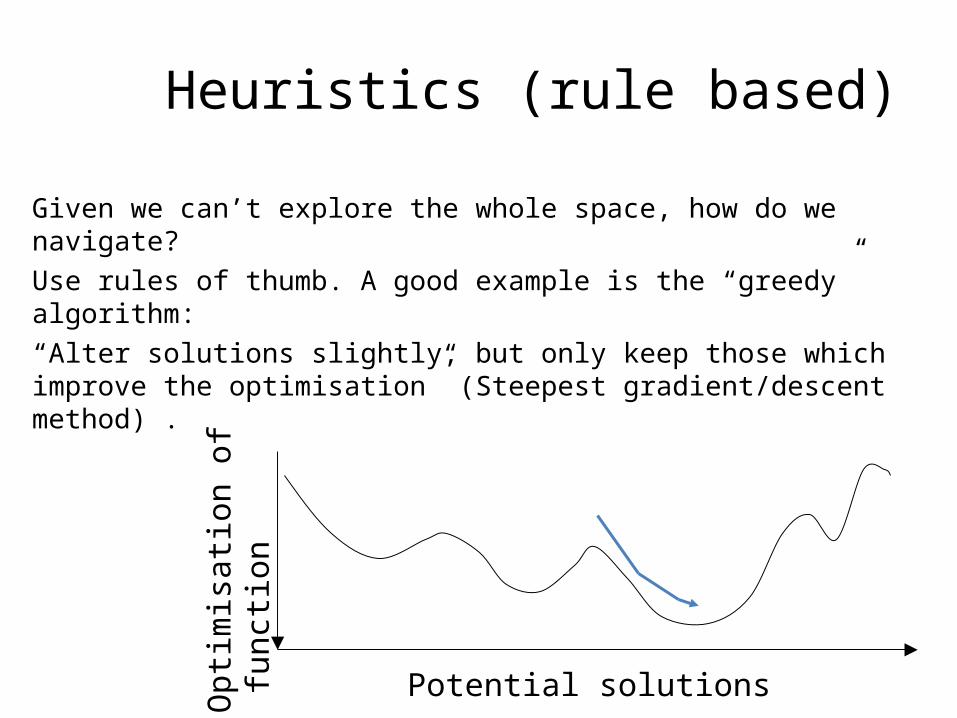
Heuristics (rule based)

Given we can’t explore the whole space, how do we navigate?Use rules of thumb. A good example is the “greedy” algorithm:“Alter solutions slightly, but only keep those which improve the optimisation” (Steepest gradient/descent method) .

Potential solutions

Opt

imisa

tion

of fu

nctio

n

Example: Microsimulation

Basis for many other techniques.An analysis technique on its own.Simulates individuals from aggregate data sets.Allows you to estimate numbers of people effected by policies.Could equally be used on tree species or soil types.Increasingly the starting point for ABM.

How?

Combines anonymised individual-level samples with aggregate population figures. Take known individuals from small scale surveys.

British Household Panel SurveyBritish Crime SurveyLifestyle databases

Take aggregate statistics where we don’t know about individuals.

UK CensusCombine them on the basis of as many variables as they share.

MicroSimulationRandomly put individuals into an area until the population numbers match.Swap people out with others while it improves the match between the real aggregate variables and the synthetic population. Use these to model direct effects.

If we have distance to work data and employment, we can simulate people who work in factory X in ED Y.

Use these to model multiplier effects.If the factory shuts down, and those people are unemployed, and their money lost from that ED, how many people will the local supermarket sack?

Heuristics (rule based)

“Alter solutions slightly, but only keep those which improve the optimisation” (Steepest gradient/descent method) .Finds a solution, but not necessarily the “best”.

Zoning scheme

Opt

imisa

tion

of fu

nctio

n

Local minima Global minimum(lowest)Stuck!

Meta-heuristic optimisation

Randomisation

Simulated annealing

Genetic Algorithm/Programming

Typical method: Randomisation

Randomise starting point.Randomly change values, but only keep those that optimise our function.Repeat and keep the best result. Aims to find the global minimum by randomising starts.

Simulated Annealing (SA)

Based on the cooling of metals, but replicates the intelligent notion that trying non-optimal solutions can be beneficial.

As the temperature drops, so the probability of metal atoms freezing where they are increases, but there’s still a chance they’ll move elsewhere.

The algorithm moves freely around the solution space, but the chances of it following a non-improving path drop with “temperature” (usually time).

In this way there’s a chance early on for it to go into less-optimal areas and find the global minimum.

But how is the probability determined?

The Metropolis Algorithm

Probability of following a worse path…

P = exp[ -(drop in optimisation / temperature)]

(This is usually compared with a random number)

Paths that increase the optimisation are always followed.

The “temperature” change varies with implementation, but broadly decreases with time or area searched.

Picking this is the problem: too slow a decrease and it’s computationally expensive, too fast and the solution isn’t good.

P

T

Genetic Algorithms (GA)

In the 1950’s a number of people tried to use evolution to solve problems.

The main advances were completed by John Holland in the mid-60’s to 70’s.

He laid down the algorithms for problem solving with evolution – derivatives of these are known as Genetic Algorithms.

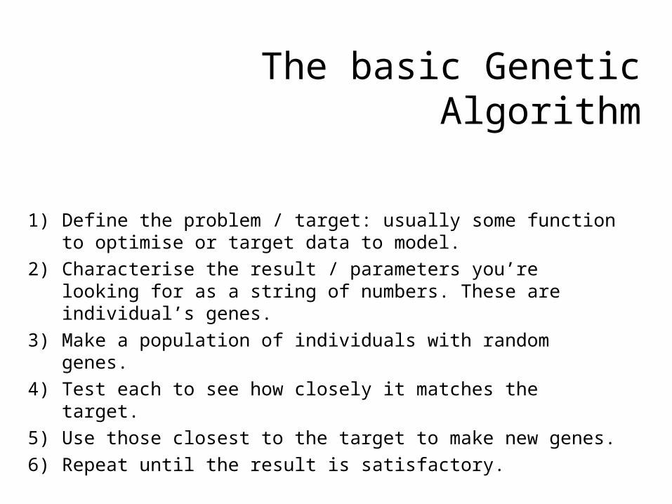
The basic Genetic Algorithm

1) Define the problem / target: usually some function to optimise or target data to model.

2) Characterise the result / parameters you’re looking for as a string of numbers. These are individual’s genes.

3) Make a population of individuals with random genes.4) Test each to see how closely it matches the target.5) Use those closest to the target to make new genes.6) Repeat until the result is satisfactory.

A GA exampleSay we have a valley profile we want to model as an equation.We know the equation is in the form…

y = a + b + c2 + d3.

We can model our solution as a string of four numbers, representing a, b, c and d.We randomise this first (e.g. to get “1 6 8 5”), 30 times to produce a population of thirty different random individuals.

We work out the equation for each, and see what the residuals are between the predicted and real valley profile.We keep the best genes, and use these to make the next set of genes.How do we make the next genes?

Inheritance, cross-over reproduction and mutation

We use the best genes to make the next population.We take some proportion of the best genes and randomly cross-over portions of them. 16|85 16|37 39|37 39|85We allow the new population to inherit these combined best genes (i.e. we copy them to make the new population).We then randomly mutate a few genes in the new population. 1637 1737

Other details

Often we don’t just take the best – we jump out of local minima by taking worse solutions.Usually this is done by setting the probability of taking a gene into the next generation as based on how good it is.

The solutions can be letters as well (e.g. evolving sentences) or true / false statements.The genes are usually represented as binary figures, and switched between one and zero.

E.g. 1 | 7 | 3 | 7 would be 0001 | 0111 | 0011 | 0111

Can we evolve anything else?

In the late 80’s a number of researchers, most notably John Koza and Tom Ray came up with ways of evolving equations and computer programs.

This has come to be known as Genetic Programming.

Genetic Programming aims to free us from the limits of our feeble brains and our poor understanding of the world, and lets something else work out the solutions.

Genetic Programming (GP)

Essentially similar to GAs only the components aren’t just the parameters of equations, they’re the whole thing.

They can even be smaller programs or the program itself.

Instead of numbers, you switch and mutate…Variables, constants and operators in equations.Subroutines, code, parameters and loops in programs.

All you need is some measure of “fitness”.

Advantages of GP and GA

Gets us away from human limited knowledge.Finds near-optimal solutions quickly.Relatively simple to program.Don’t need much setting up.

Disadvantages of GP and GA

The results are good representations of reality, but they’re often impossible to relate to physical / causal systems. E.g. river level = (2.443 x rain) rain-2 + ½ rain + 3.562

GPs have to be reassessed entirely to adapt to changes in the target data if it comes from a dynamic system.

Tend to be good at finding initial solutions, but slow to become very accurate – often used to find initial states for other AI techniques.

Uses in ABM

Behavioural modelsEvolve Intelligent Agents that respond to modelled economic and

environmental situations realistically.(Most good conflict-based computer games have GAs driving the

enemies so they adapt to changing player tactics)

Heppenstall (2004); Kim (2005)Calibrating models

Other uses

As well as searches in solution space, we can use these techniques to search in other spaces as well.

Searches for troughs/peaks (clusters) of a variable in geographical space.

e.g. cancer incidences.

Searches for troughs (clusters) of a variable in variable space.e.g. groups with similar travel times to work.

Identifiability

It may be that multiple sets of parameters would give a model that matched the calibration data well, but gave varying predictive results. Whether we can identify the true parameters from the data is known as the identifiability problem. Discovering what these parameters are is the inverse problem.

If we can’t identify the true parameter sets, we may want to Monte Carlo test the distribution of potential parameter sets to show the range of potential solutions.

Equifinality

In addition, we may not trust the model form because multiple models give the same calibration results (the equifinality problem).

We may want to test multiple model forms against each other and pick the best (e.g. GLUE methodology).

Or we may want to combine the results if we think different system components are better represented by different models.

Some evidence that such ‘ensemble’ models do better.

Either way…

Both the equifinality issue and the inverse problem mean we will have to run large numbers of models…