California State Waters Map Series—Offshore of Fort Ross, California

By Samuel Y. Johnson, Peter Dartnell, Nadine E. Golden, Stephen R. Hartwell, Mercedes D. Erdey, H. Gary Greene, Guy R. Cochrane, Rikk G. Kvitek, Michael W. Manson, Charles A. Endris, Bryan E. Dieter, Janet T. Watt, Lisa M. Krigsman, Ray W. Sliter, Erik N. Lowe, and John L. Chin

(Samuel Y. Johnson and Susan A. Cochran, editors)

Pamphlet to accompany

Open-File Report 2015–1211

2015

U.S. Department of the Interior U.S. Geological Survey

U.S. Department of the Interior SALLY JEWELL, Secretary

U.S. Geological Survey Suzette M. Kimball, Acting Director

U.S. Geological Survey, Reston, Virginia: 2015

For more information on the USGS—the Federal source for science about the Earth, its natural and living resources, natural hazards, and the environment—visit http://www.usgs.gov or call 1–888–ASK–USGS (1–888–275–8747).

For an overview of USGS information products, including maps, imagery, and publications, visit http://www.usgs.gov/pubprod/.

To order this and other USGS information products, visit http://store.usgs.gov/.

Any use of trade, firm, or product names is for descriptive purposes only and does not imply endorsement by the U.S. Government.

Although this information product, for the most part, is in the public domain, it also may contain copyrighted materials as noted in the text. Permission to reproduce copyrighted items must be secured from the copyright owner.

Suggested citation: Johnson, S.Y., Dartnell, P., Golden, N.E., Hartwell, S.R., Erdey, M.D., Greene, H.G., Cochrane, G.R., Kvitek, R.G., Manson, M.W., Endris, C.A., Dieter, B.E., Watt, J.T., Krigsman, L.M., Sliter, R.W., Lowe, E.N., and Chin, J.L. (S.Y. Johnson and S.A. Cochran, eds.), 2015, California State Waters Map Series—Offshore of Fort Ross, California: U.S. Geological Survey Open-File Report 2015–1211, pamphlet 37 p., 10 sheets, scale 1:24,000, http://dx.doi.org/10.3133/ofr20151211.

ISSN 2331-1258 (online)

iii

Contents Preface ........................................................................................................................................................................... 1 Chapter 1. Introduction ................................................................................................................................................... 3

By Samuel Y. Johnson Regional Setting ......................................................................................................................................................... 3 Publication Summary .................................................................................................................................................. 5

Chapter 2. Bathymetry and Backscatter-Intensity Maps of the Offshore of Fort Ross Map Area (Sheets 1, 2, and 3) ... 8 By Peter Dartnell and Rikk G. Kvitek

Chapter 3. Data Integration and Visualization for the Offshore of Fort Ross Map Area (Sheet 4) ................................ 10 By Peter Dartnell

Chapter 4. Seafloor-Character Map of the Offshore of Fort Ross Map Area (Sheet 5) ................................................ 11 By Mercedes D. Erdey and Guy R. Cochrane

Chapter 5. Ground-Truth Studies for the Offshore of Fort Ross Map Area (Sheet 6) ................................................... 15 By Nadine E. Golden and Guy R. Cochrane

Chapter 6. Potential Marine Benthic Habitats of the Offshore of Fort Ross Map Area (Sheet 7) ................................. 18 By H. Gary Greene, Charles A. Endris, and Bryan E. Dieter

Classifying Potential Marine Benthic Habitats .......................................................................................................... 18 Examples of Attribute Coding ................................................................................................................................... 20 Map Area Habitats .................................................................................................................................................... 20

Chapter 7. Subsurface Geology and Structure of the Offshore of Fort Ross Map Area and the Salt Point to Drakes Bay Region (Sheets 8 and 9) ....................................................................................................................................... 21

By Samuel Y. Johnson, Stephen R. Hartwell, and Janet T. Watt Data Acquisition........................................................................................................................................................ 21 Seismic-Reflection Imaging of the Continental Shelf ................................................................................................ 21 Geologic Structure and Recent Deformation ............................................................................................................ 23 Thickness and Depth to Base of Uppermost Pleistocene and Holocene Deposits ................................................... 24

Chapter 8. Geologic and Geomorphic Map of the Offshore of Fort Ross Map Area (Sheet 10) ................................... 26 By Samuel Y. Johnson, Michael W. Manson, and Stephen R. Hartwell

Geologic and Geomorphic Summary ........................................................................................................................ 26 Description of Map Units .......................................................................................................................................... 29

Offshore Geologic and Geomorphic Units ............................................................................................................ 29 Onshore Geologic and Geomorphic Units ............................................................................................................ 30

Acknowledgments ........................................................................................................................................................ 32 References Cited ......................................................................................................................................................... 33

Figures Figure 1–1. Physiography of northern California coast from Point Arena to San Francisco........................................... 6 Figure 1–2. Coastal geography of Offshore of Fort Ross map area .............................................................................. 7 Figure 4–1. Detailed view of ground-truth data, showing accuracy-assessment methodology .................................... 13 Figure 5–1. Photograph of camera sled used in USGS 2008 ground-truth survey ...................................................... 15 Figure 5–2. Graph showing distribution of primary and secondary substrate determined from video observations in

Offshore of Fort Ross map area ............................................................................................................... 17

iv

Tables Table 4–1. Conversion table showing how video observations of primary substrate, secondary substrate, and

abiotic seafloor complexity are grouped into seafloor-character-map Classes I, II, III, and IV for use in supervised classification and accuracy assessment in Offshore of Fort Ross map area .......................... 14

Table 4–2. Accuracy-assessment statistics for seafloor-character-map classifications in Offshore of Fort Ross map area .......................................................................................................................................................... 14

Table 7–1. Area, sediment-thickness, and sediment-volume data for California’s State Waters in Salt Point to Drakes Bay region, as well as in Offshore of Fort Ross map area............................................................ 25

Table 8–1. Areas and relative proportions of offshore geologic map units in Offshore of Fort Ross map area .......... 28

Map Sheets Sheet 1. Colored Shaded-Relief Bathymetry, Offshore of Fort Ross Map Area, California

By Peter Dartnell and Rikk G. Kvitek Sheet 2. Shaded-Relief Bathymetry, Offshore of Fort Ross Map Area, California

By Peter Dartnell and Rikk G. Kvitek Sheet 3. Acoustic Backscatter, Offshore of Fort Ross Map Area, California

By Peter Dartnell, Mercedes D. Erdey, and Rikk G. Kvitek Sheet 4. Data Integration and Visualization, Offshore of Fort Ross Map Area, California

By Peter Dartnell Sheet 5. Seafloor Character, Offshore of Fort Ross Map Area, California

By Mercedes D. Erdey and Guy R. Cochrane Sheet 6. Ground-Truth Studies, Offshore of Fort Ross Map Area, California

By Nadine E. Golden, Guy R. Cochrane, and Lisa M. Krigsman Sheet 7. Potential Marine Benthic Habitats, Offshore of Fort Ross Map Area, California

By Bryan E. Dieter, H. Gary Greene, Charles A. Endris, Mercedes D. Erdey, and Erik M. Lowe Sheet 8. Seismic-Reflection Profiles, Offshore of Fort Ross Map Area, California

By Samuel Y. Johnson, Ray W. Sliter, Stephen R. Hartwell, and John L. Chin Sheet 9. Local (Offshore of Fort Ross Map Area) and Regional (Offshore from Salt Point to Drakes Bay)

Shallow-Subsurface Geology and Structure, California By Samuel Y. Johnson, Stephen R. Hartwell, Janet T. Watt, and Ray W. Sliter

Sheet 10. Offshore and Onshore Geology and Geomorphology, Offshore of Fort Ross Map Area, California By Samuel Y. Johnson, Stephen R. Hartwell, and Michael W. Manson

1

California State Waters Map Series—Offshore of Fort Ross, California

By Samuel Y. Johnson,1 Peter Dartnell,1 Nadine E. Golden,1 Stephen R. Hartwell,1 Mercedes D. Erdey,1 H. Gary Greene,2 Guy R. Cochrane,1 Rikk G. Kvitek,3 Michael W. Manson,4 Charles A. Endris,2 Bryan E. Dieter,2 Janet T. Watt,1 Lisa M. Krigsman,5 Ray W. Sliter,1 Erik N. Lowe,1 and John L. Chin1

(Samuel Y. Johnson1 and Susan A. Cochran,1 editors)

Preface In 2007, the California Ocean Protection Council initiated the California Seafloor Mapping

Program (CSMP), designed to create a comprehensive seafloor map of high-resolution bathymetry, marine benthic habitats, and geology within California’s State Waters. The program supports a large number of coastal-zone- and ocean-management issues, including the California Marine Life Protection Act (MLPA) (California Department of Fish and Wildlife, 2008), which requires information about the distribution of ecosystems as part of the design and proposal process for the establishment of Marine Protected Areas. A focus of CSMP is to map California’s State Waters with consistent methods at a consistent scale.

The CSMP approach is to create highly detailed seafloor maps through collection, integration, interpretation, and visualization of swath sonar data (the undersea equivalent of satellite remote-sensing data in terrestrial mapping), acoustic backscatter, seafloor video, seafloor photography, high-resolution seismic-reflection profiles, and bottom-sediment sampling data. The map products display seafloor morphology and character, identify potential marine benthic habitats, and illustrate both the surficial seafloor geology and shallow (to about 100 m) subsurface geology. It is emphasized that the more interpretive habitat and geology maps rely on the integration of multiple, new high-resolution datasets and that mapping at small scales would not be possible without such data.

This approach and CSMP planning is based in part on recommendations of the Marine Mapping Planning Workshop (Kvitek and others, 2006), attended by coastal and marine managers and scientists from around the state. That workshop established geographic priorities for a coastal mapping project and identified the need for coverage of “lands” from the shore strand line (defined as Mean Higher High Water; MHHW) out to the 3-nautical-mile (5.6-km) limit of California’s State Waters. Unfortunately, surveying the zone from MHHW out to 10-m water depth is not consistently possible using ship-based surveying methods, owing to sea state (for example, waves, wind, or currents), kelp coverage, and shallow rock outcrops. Accordingly, some of the maps presented in this series commonly do not cover the zone from the shore out to 10-m depth; these “no data” zones appear pale gray on most maps.

This map is part of a series of online U.S. Geological Survey (USGS) publications, each of which includes several map sheets, some explanatory text, and a descriptive pamphlet. Each map sheet

1 U.S. Geological Survey 2 Moss Landing Marine Laboratories, Center for Habitat Studies 3 California State University, Monterey Bay, Seafloor Mapping Lab 4 California Geological Survey 5 National Oceanic and Atmospheric Administration, National Marine Fisheries Service

2

is published as a PDF file. Geographic information system (GIS) files that contain both ESRI6 ArcGIS raster grids (for example, bathymetry, seafloor character) and geotiffs (for example, shaded relief) are also included for each publication. For those who do not own the full suite of ESRI GIS and mapping software, the data can be read using ESRI ArcReader, a free viewer that is available at http://www.esri.com/software/arcgis/arcreader/index.html (last accessed February 5, 2014).

The California Seafloor Mapping Program (CSMP) is a collaborative venture between numerous different federal and state agencies, academia, and the private sector. CSMP partners include the California Coastal Conservancy, the California Ocean Protection Council, the California Department of Fish and Wildlife, the California Geological Survey, California State University at Monterey Bay’s Seafloor Mapping Lab, Moss Landing Marine Laboratories Center for Habitat Studies, Fugro Pelagos, Pacific Gas and Electric Company, National Oceanic and Atmospheric Administration (NOAA, including National Ocean Service – Office of Coast Surveys, National Marine Sanctuaries, and National Marine Fisheries Service), U.S. Army Corps of Engineers, the Bureau of Ocean Energy Management, the National Park Service, and the U.S. Geological Survey.

6 Environmental Systems Research Institute, Inc.

3

Chapter 1. Introduction By Samuel Y. Johnson

Regional Setting The map area offshore of Fort Ross, California, which is referred to herein as the “Offshore of

Fort Ross” map area (figs. 1–1, 1–2) is located in northern California, on the Pacific coast of Sonoma County, about 90 km north of San Francisco and 60 km south of Point Arena (fig. 1–1). The onshore part of the map area is largely undeveloped, used primarily for grazing and recreation; the small town of Jenner (population, 136), located at the mouth of the Russian River (fig. 1–2), is the largest cultural center. The coast and shoreline are rugged and scenic, characterized by rocky promontories, kelp-rich coves, and nearshore rocks and sea stacks. U.S. Highway 1 extends along the coast through the map area, crossing the Russian River and passing through Sonoma Coast State Park and Fort Ross State Historic Park. Sonoma Coast State Park is a series of beaches separated by rocky bluffs and headlands that extends from about 27 km north of Bodega Head to about 6 km north of the Russian River (fig. 1–1).

Fort Ross is both a California Historical Landmark and a National Historic Landmark, and it is on the National Register of Historic Places. It was established in 1812 and served as a thriving Russian-American Company settlement until 1841 (California Department of Parks and Recreation, 2013). The company used Fort Ross as an agricultural base, supplying Russian settlements in Alaska and the northeast Pacific. Fort Ross was sold in 1841 when more northern settlements took over this role. In 1906, the stockade and some surrounding land were acquired by the State of California for preservation as a historic monument. Subsequently, more of the surrounding land was obtained, and Fort Ross Historic State Park was established.

The Offshore of Fort Ross map area is cut by the northwest-striking San Andreas Fault (fig. 1–1), the right-lateral transform boundary between the North American and Pacific plates. The fault intersects the shoreline a few kilometers south of Fort Ross at Timber Gulch, and it juxtaposes Jurassic, Cretaceous, Paleocene, and Eocene rocks of the Franciscan Complex to the northeast and Tertiary sedimentary rocks to the southwest (sheet 10 of this report). In this area, the San Andreas Fault has an estimated slip rate of 17 to 24 mm/yr (U.S. Geological Survey and California Geological Survey, 2010). The devastating great 1906 California earthquake (M7.8) is thought to have nucleated on the San Andreas Fault offshore of San Francisco (see, for example, Bolt, 1968; Lomax, 2005), about 90 km to the south, with the rupture extending northward through the Offshore of Fort Ross map area to the south flank of Cape Mendocino. Approximately 3.6 m of lateral offset occurred at Timber Gulch during this event (Brown and Wolfe, 1972).

The San Andreas Fault has an important influence on coastal geomorphology (fig. 1–2). The coastline in the northern part of the map area, southwest of the onshore San Andreas Fault, is characterized by steep shoreline bluffs and as many as four uplifted, relatively flat marine terraces that range in elevation from about 15 to 100 m (Prentice and Kelson, 2006). Northeast of the San Andreas Fault, in the southern part of the map area, about 12 km of coastline is marked by steep, landslide-prone cliffs that commonly are 200 to 300 m high. This steep coastal topography tapers off to the south, and low marine terraces (about 15 to 30 m high) are present along the southern about 2 km of shoreline.

The mouth of the Russian River and its estuary cut through the steep coastal topography in the southern part of the map area (fig. 1–2). The Russian River drains a large watershed (3,470 km2), and it has an annual discharge of about 2 km3 (1,600,000 acre-feet) and an annual sediment load of about 900,000 metric tons (Farnsworth and Warrick, 2007).

4

Habel and Armstrong (1978) and Hapke and others (2006) considered the Offshore of Fort Ross map area to be part of the Russian River littoral cell, in which the predominant longshore drift is to the south. They noted that the area is dominated by small pocket beaches, but they reported that some of the longer linear beaches near the mouth of the Russian River had long-term (1862–2002) rates of shoreline change that range from about 0.4 m/yr (accretion) to -0.7 m/yr (erosion); they also reported short-term (1952–2002) rates of shoreline change that range from about 2.5 m/yr (accretion) to -1.5 m/yr (erosion).

The seafloor in the north half of the map area is characterized by rocky outcrops of Tertiary sedimentary rocks. The rugged nearshore zone and the inner shelf area (to water depths of about 50 m) typically dip gently seaward (about 1.5° to 2.5°), whereas the smooth midshelf area within California’s State Waters (about 50 to 85 m deep) is relatively flat (about 0.4°). In contrast, the nearshore to midshelf area in the south half of the map area, which lies directly offshore of the mouth of the Russian River, has a more uniform dip: about 0.45° out to water depths of about 30 m and about 0.65° to 0.8° at water depths from 30 to 70 m. Shallow-marine and shelf sediments were deposited in the last about 21,000 years during the sea-level rise that followed the Last Glacial Maximum (LGM; Fairbanks, 1989; Fleming and others, 1998; Lambeck and Chappell, 2001; Peltier and Fairbanks, 2006). Sea level was about 125 m lower than present during the LGM, at which time the entire Offshore of Fort Ross map area was emergent and the shoreline was about 20 km west of its present location.

Circulation over the continental shelf in the map area (and in the broader northern California region) is dominated by the southward-flowing California Current, the eastern limb of the North Pacific Gyre (Hickey, 1979). Associated upwelling brings cool, nutrient-rich waters to the surface, resulting in high biological productivity. The current flow generally is southeastward during the spring and summer; however, during the fall and winter, the otherwise persistent northwest winds are sometimes weak or absent, causing the California Current to move farther offshore and the Davidson Current, a weaker, northward-flowing countercurrent (Hickey, 1979), to become active.

Throughout the year, this part of the northern California coast is exposed to four wave climate regimes: the north Pacific swell, the southern swell, northwest wind waves, and local wind waves (Storlazzi and Griggs, 2000; Storlazzi and Wingfield, 2005). The north Pacific swell dominates in winter months (typically, November through March), with wave heights at offshore buoys ranging from 2 to 10 m and wave periods ranging from 10 to 25 s (Storlazzi and Wingfield, 2005). During summer months, the largest waves come from the southern swell, generated by storms in the south Pacific and offshore of Central America. Characteristically, these swells have smaller wave heights (0.3–3 m) and similarly long wave periods (10–25 s). Northwest wind waves affect the coast throughout the year, whereas local wind waves are most common from October to April. These two wind-wave regimes typically have wave heights of 1 to 4 m and short wave periods (3–10 s).

Common potential marine benthic habitat types in the Offshore of Fort Ross map area include unconsolidated continental-shelf sediments, mixed continental-shelf substrate, and hard continental-shelf substrate. Rocky shelf outcrops and rubble are considered the primary habitat type for rockfish (Sebastes spp.) and lingcod (Ophiodon elongatus) (Cass and others, 1990; Love and others, 2002), both of which are recreationally and commercially important species.

The Offshore of Fort Ross map area includes two California Marine Protected Areas (MPAs; California Department of Fish and Wildlife, 2012). MPAs are named, discrete geographic marine or estuarine areas seaward of the mean high tide line or the mouth of a coastal river, including any area of intertidal or subtidal terrain. These areas, including their overlying water and associated flora and fauna, have been designated by law or administrative action for the purpose of protecting or conserving marine life and habitat. There are four types of MPAs in California: State Marine Reserve (SMR), State Marine Park (SMP), State Marine Conservation Area (SMCA), and Special Closure (SC). The Offshore of Fort Ross map area includes the Russian River State Marine Conservation Area (offshore) and the Russian

5

River State Marine Recreational Management Area, which includes part of the estuary between the mouth of the Russian River and the bridge crossing at U.S. Highway 1 (fig. 1–2).

Publication Summary This publication about the Offshore of Fort Ross map area includes ten map sheets that contain

explanatory text, in addition to this descriptive pamphlet and a data catalog of geographic information system (GIS) files. Sheets 1, 2, and 3 combine data from four different sonar surveys to generate comprehensive high-resolution bathymetry and acoustic backscatter coverage of the map area. These data reveal a range of physiographic features (highlighted in the perspective views on sheet 4) such as the smooth seafloor of the offshore Russian River delta, rugged nearshore bedrock outcrops, shallow “scour depressions,” and sediment lobes inferred to have formed by ground failure associated with strong ground motions on the nearby San Andreas Fault. To validate the geological and biological interpretations of the sonar data shown in sheets 1, 2, and 3, the U.S. Geological Survey towed a camera sled over specific offshore locations, collecting both video and photographic imagery; this “ground-truth” surveying data is summarized on sheet 6. Sheet 5 is a “seafloor character” map, which classifies the seafloor on the basis of depth, slope, rugosity (ruggedness), and backscatter intensity and which is further informed by the ground-truth-survey imagery. Sheet 7 is a map of “potential habitats,” which are delineated on the basis of substrate type, geomorphology, seafloor process, or other attributes that may provide a habitat for a specific species or assemblage of organisms. Sheet 8 compiles representative seismic-reflection profiles from the map area, providing information on the subsurface stratigraphy and structure of the map area. Sheet 9 shows the distribution and thickness of young sediment (deposited over the last about 21,000 years, during the most recent sea-level rise) in both the map area and the larger Salt Point to Drakes Bay region, interpreted on the basis of the seismic-reflection data, and it identifies the Offshore of Fort Ross map area as lying within the Salt Point shelf and Russian River delta and mud belt domains. Sheet 10 is a geologic map that merges onshore geologic mapping (compiled from existing maps by the California Geological Survey) and new offshore geologic mapping that is based on the integration of high-resolution bathymetry and backscatter imagery (sheets 1, 2, 3), seafloor-sediment and rock samples (Reid and others, 2006), digital camera and video imagery (sheet 6), and high-resolution seismic-reflection profiles (sheet 8).

The information provided by the map sheets, pamphlet, and data catalog has a broad range of applications. High-resolution bathymetry, acoustic backscatter, ground-truth-surveying imagery, and habitat mapping all contribute to habitat characterization and ecosystem-based management by providing essential data for delineation of marine protected areas and ecosystem restoration. Many of the maps provide high-resolution baselines that will be critical for monitoring environmental change associated with climate change, coastal development, or other forcings. High-resolution bathymetry is a critical component for modeling coastal flooding caused by storms and tsunamis, as well as inundation associated with longer term sea-level rise. Seismic-reflection and bathymetric data help characterize earthquake and tsunami sources, critical for natural-hazard assessments of coastal zones. Information on sediment distribution and thickness is essential to the understanding of local and regional sediment transport, as well as the development of regional sediment-management plans. In addition, siting of any new offshore infrastructure (for example, pipelines, cables, or renewable-energy facilities) will depend on high-resolution mapping. Finally, this mapping will both stimulate and enable new scientific research and also raise public awareness of, and education about, coastal environments and issues.

6

Figure 1–1. Physiography of northern California coast from Point Arena to San Francisco (SF). Red box shows Offshore of Fort Ross map area. Yellow line shows limit of California’s State Waters. Black line shows San Andreas Fault (SAF). Other abbreviations: PR, Point Reyes peninsula; TP, Tomales Point.

7

Figure 1–2. Coastal geography of Offshore of Fort Ross map area. Yellow line shows limit of California’s State Waters. Dashed white line shows boundary of Russian River State Marine Conservation Area (RCA). Other abbreviations: FR, Fort Ross; J, Jenner; RR, Russian River; TC, Timber Cove Creek; TG, Timber Gulch.

8

Chapter 2. Bathymetry and Backscatter-Intensity Maps of the Offshore of Fort Ross Map Area (Sheets 1, 2, and 3) By Peter Dartnell and Rikk G. Kvitek

The colored shaded-relief bathymetry (sheet 1), the shaded-relief bathymetry (sheet 2), and the acoustic-backscatter (sheet 3) maps of the Offshore of Fort Ross map area in northern California were generated from bathymetry and backscatter data collected by Fugro Pelagos and by California State University, Monterey Bay (CSUMB) (fig. 1 on sheets 1, 2, 3). Mapping was completed between 2007 and 2010, using a combination of 200-kHz and 400-kHz Reson 7125 and 244-kHz Reson 8101 multibeam echosounders, as well as a 468-kHz SEA SWATHplus bathymetric sidescan-sonar system. These mapping missions combined to collect both bathymetry (sheets 1, 2) and acoustic-backscatter data (sheet 3) from about the 10-m isobath to beyond the 3-nautical-mile limit of California’s State Waters.

During the mapping missions, an Applanix POS MV (Position and Orientation System for Marine Vessels) was used to accurately position the vessels during data collection, and it also accounted for vessel motion such as heave, pitch, and roll (position accuracy, ±2 m; pitch, roll, and heading accuracy, ±0.02°; heave accuracy, ±5%, or 5 cm). To account for tidal-cycle fluctuations, CSUMB used NavCom 2050 GPS receiver (CNAV) data, and Fugro Pelagos used KGPS data (GPS data with real-time kinematic corrections); in addition, sound-velocity profiles were collected with an Applied Microsystems (AM) SVPlus sound velocimeter. Soundings were corrected for vessel motion using the Applanix POS MV data, for variations in water-column sound velocity using the AM SVPlus data, and for variations in water height (tides) using vertical-position data from the KGPS receivers.

The multibeam-echosounder backscatter data were postprocessed using CARIS 7.0/Geocoder software. Within Geocoder, the backscatter intensities were radiometrically corrected (including despeckling and angle-varying gain adjustments), and the position of each acoustic sample was geometrically corrected for slant range on a line-by-line basis. After the lines were corrected, they were mosaicked into a 1-m-resolution image. Overlap between parallel lines was resolved using a priority table whose values were based on the distance of each sample from the ship track, with the samples that were closest to and furthest from the ship track being given the lowest priority. An anti-aliasing algorithm was also applied. The mosaics were then exported as georeferenced TIFF images, imported into a geographic information system (GIS), and converted to GRIDs at 2-m resolution.

The SWATHplus backscatter data were postprocessed using USGS software (D.P. Finlayson, written commun., 2011) that normalizes for time-varying signal loss and beam-directivity differences. Thus, the raw 16-bit backscatter data were gain-normalized to enhance the backscatter of the SWATHplus system. The resulting normalized-amplitude values were rescaled to 16-bit and gridded into GeoJPEGs using GRID Processor Software, then imported into a GIS and converted to GRIDs.

Processed soundings from the different mapping missions were exported from the acquisition or processing software as XYZ files and bathymetric surfaces. All the surfaces were merged into one overall 2-m-resolution bathymetric-surface model and clipped to the boundary of the map area. An illumination having an azimuth of 300° and from 45° above the horizon was then applied to the bathymetric surface to create the shaded-relief imagery (sheets 1, 2). In addition, a modified “rainbow” color ramp was applied to the bathymetry data for sheet 1, using reds and oranges to represent shallower depths, and purples to represent greater depths. This colored bathymetry surface was draped over the shaded-relief imagery at 60-percent transparency to create a colored shaded-relief map (sheet 1). Note that the ripple patterns and straight lines that are apparent within the map area are data-collection artifacts. In addition, lines at the borders of some surveys are the result of slight differences in depth, as

9

measured by different mapping systems in different years. These various artifacts are made obvious by the hillshading process.

Bathymetric contours (sheets 1, 2, 3, 5, 7, 10) were generated at 10-m intervals from the merged 2-m-resolution bathymetric surface. The merged surface was smoothed using the Focal Mean tool in ArcGIS and a circular neighborhood that has a radius of between 20 and 30 m (depending on the location). The contours were generated from this smoothed surface using the Spatial Analyst Contour tool in ArcGIS. The most continuous contour segments were preserved; smaller segments and isolated island polygons were excluded from the final output. The contours were then clipped to the boundary of the map area.

The acoustic-backscatter imagery from each different mapping system and processing method were merged into their own individual grids. These individual grids, which cover different areas, were displayed in a GIS to create a composite acoustic-backscatter map (sheet 3). On the map, brighter tones indicate higher backscatter intensity, and darker tones indicate lower backscatter intensity. The intensity represents a complex interaction between the acoustic pulse and the seafloor, as well as characteristics within the shallow subsurface, providing a general indication of seafloor texture and sediment type. Backscatter intensity depends on the acoustic source level; the frequency used to image the seafloor; the grazing angle; the composition and character of the seafloor, including grain size, water content, bulk density, and seafloor roughness; and some biological cover. Harder and rougher bottom types such as rocky outcrops or coarse sediment typically return stronger intensities (high backscatter, lighter tones), whereas softer bottom types such as fine sediment return weaker intensities (low backscatter, darker tones). The differences in backscatter intensity that are apparent in some areas on sheet 3 are due to the different frequencies of mapping systems, as well as different processing techniques. Note that the parallel lines of higher backscatter intensity throughout the map area are data-collection artifacts.

The onshore-area image was generated by applying an illumination having an azimuth of 300° and from 45° above the horizon to 2-m-resolution topographic-lidar data from National Oceanic and Atmospheric Administration’s (NOAA’s) Digital Coast (available at http://coast.noaa.gov/digitalcoast/ data/coastallidar/) and from OpenTopography (available at http://www.opentopography.org/), as well as to 10-m-resolution topographic-lidar data from the U.S. Geological Survey’s National Elevation Dataset (available at http://ned.usgs.gov).

10

Chapter 3. Data Integration and Visualization for the Offshore of Fort Ross Map Area (Sheet 4) By Peter Dartnell

Mapping California’s State Waters has produced a vast amount of acoustic and visual data, including bathymetry, acoustic backscatter, seismic-reflection profiles, and seafloor video and photography. These data are used by researchers to develop maps, reports, and other tools to assist in the coastal and marine spatial-planning capability of coastal-zone managers and other stakeholders. For example, seafloor-character (sheet 5), habitat (sheet 7), and geologic (sheet 10) maps of the Offshore of Fort Ross map area may assist in the designation of Marine Protected Areas, as well as in their monitoring. These maps and reports also help to analyze environmental change owing to sea-level rise and coastal development, to model and predict sediment and contaminant budgets and transport, to site offshore infrastructure, and to assess tsunami and earthquake hazards. To facilitate this increased understanding and to assist in product development, it is helpful to integrate the different datasets and then view the results in three-dimensional representations such as those displayed on the data integration and visualization sheet for the Offshore of Fort Ross map area (sheet 4).

The maps and three-dimensional views on sheet 4 were created using a series of geographic information systems (GIS) and visualization techniques. Using GIS, the bathymetric and topographic data (sheet 1) were converted to ASCIIRASTER format files, and the acoustic-backscatter data (sheet 3) were converted to geoTIFF images. The bathymetric and topographic data were imported in the Fledermaus® software (QPS). The bathymetry was color-coded to closely match the colored shaded-relief bathymetry on sheet 1, in which reds and oranges represent shallower depths and purples represent deeper depths. Topographic data were shown in gray shades. The acoustic-backscatter geoTIFF images were also draped over the bathymetry data. The colored bathymetry, topography, and draped backscatter were then tilted and panned to create the perspective views such as those shown in figures 1 through 6 on sheet 4. These figures highlight the seafloor morphology in the Offshore of Fort Ross map area, which includes outcrops of fractured bedrock and complex patterns of shallow depressions.

Block diagrams that combine the bathymetry with seismic-reflection-profile data help integrate surface and subsurface observations, especially stratigraphic and structural relations (for example, fig. 6 on sheet 4). These block diagrams were created by converting digital seismic-reflection-profile data (see sheet 8) into TIFF images, while taking note of the starting and ending coordinates and maximum and minimum depths. The images were then imported into the Fledermaus® software as vertical images and merged with the bathymetry imagery.

11

Chapter 4. Seafloor-Character Map of the Offshore of Fort Ross Map Area (Sheet 5) By Mercedes D. Erdey and Guy R. Cochrane

The California State Marine Life Protection Act (MLPA) calls for protecting representative types of habitat in different depth zones and environmental conditions. A science team, assembled under the auspices of the California Department of Fish and Wildlife (CDFW), has identified seven substrate-defined seafloor habitats in California’s State Waters that can be classified using sonar data and seafloor video and photography. These habitats include rocky banks, intertidal zones, sandy or soft ocean bottoms, underwater pinnacles, kelp forests, submarine canyons, and seagrass beds. The following five depth zones, which determine changes in species composition, have been identified: Depth Zone 1, intertidal; Depth Zone 2, intertidal to 30 m; Depth Zone 3, 30 to 100 m; Depth Zone 4, 100 to 200 m; and Depth Zone 5, deeper than 200 m (California Department of Fish and Wildlife, 2008). The CDFW habitats, with the exception of depth zones, can be considered a subset of a broader classification scheme of Greene and others (1999) that has been used by the U.S. Geological Survey (USGS) (Cochrane and others, 2003, 2005). These seafloor-character maps are generalized polygon shapefiles that have attributes derived from Greene and others (2007).

A 2007 Coastal Map Development Workshop, hosted by the USGS in Menlo Park, California, identified the need for more detailed (relative to Greene and others’ [1999] attributes) raster products that preserve some of the transitional character of the seafloor when substrates are mixed and (or) they change gradationally. The seafloor-character map, which delineates a subset of the CDFW habitats, is a GIS-derived raster product that can be produced in a consistent manner from data of variable quality covering large geographic regions.

The following four substrate classes are identified in the Offshore of Fort Ross map area: • Class I: Fine- to medium-grained smooth sediment • Class II: Mixed smooth sediment and rock • Class III: Rock and boulder, rugose • Class IV: Medium- to coarse-grained sediment (in scour depressions) The seafloor-character map of the Offshore of Fort Ross map area (sheet 5) was produced using

video-supervised maximum-likelihood classification of the bathymetry and intensity of return from sonar systems, following the method described by Cochrane (2008). The two variants used in this classification were backscatter intensity and derivative rugosity. Rugosity calculation was performed using the Terrain Ruggedness (VRM) tool within the Benthic Terrain Modeler toolset v. 3.0 (Wright and others, 2012; available at http://esriurl.com/5754).

Class I, II, and III values were delineated using multivariate analysis. Class IV (medium- to coarse-grained sediment, in scour depressions) values were determined on the basis of their visual characteristics using both shaded-relief bathymetry and backscatter (slight depression in the seafloor, very high backscatter return). The resulting map (gridded at 2 m) was cleaned by hand to remove data-collection artifacts (for example, the trackline nadir).

On the seafloor-character map (sheet 5), the four substrate classes have been colored to indicate the California MLPA depth zones and the Coastal and Marine Ecological Classification Standard (CMECS) slope zones (Madden and others, 2008) in which they belong. The California MLPA depth zones are Depth Zone 1 (intertidal), Depth Zone 2 (intertidal to 30 m), Depth Zone 3 (30 to 100 m), Depth Zone 4 (100 to 200 m), and Depth Zone 5 (greater than 200 m); in the Offshore of Fort Ross map area, only Depth Zones 2 and 3 are present. The slope classes that represent the CMECS slope zones are

12

Slope Class 1 = flat (0° to 5°), Slope Class 2 = sloping (5° to 30°), Slope Class 3 = steeply sloping (30° to 60°), Slope Class 4 = vertical (60° to 90°), and Slope Class 5 = overhang (greater than 90°); in the Offshore of Fort Ross map area, only Slope Classes 1 and 2 are present. The final classified seafloor-character raster map image has been draped over the shaded-relief bathymetry for the area (sheets 1 and 2) to produce the image shown on the seafloor-character map on sheet 5.

The seafloor-character classification also is summarized on sheet 5 in table 1. Fine- to medium-grained smooth sediment (sand and mud) makes up 84.0 percent (98.3 km2) of the map area: 16.6 percent (19.4 km2) is in Depth Zone 2, and 67.4 percent (78.9 km2) is in Depth Zone 3. Mixed smooth sediment (sand and gravel) and rock (that is, sediment typically forming a veneer over bedrock, or rock outcrops having little to no relief) make up 4.9 percent (5.7 km2) of the map area: 3.1 percent (3.6 km2) is in Depth Zone 2, and 1.8 percent (2.1 km2) is in Depth Zone 3. Rock and boulder, rugose (rock and boulder outcrops having high surficial complexity) makes up 5.0 percent (5.9 km2) of the map area: 3.4 percent (4.0 km2) is in Depth Zone 2, and 1.6 percent (1.9 km2) is in Depth Zone 3. Medium- to coarse-grained sediment (in scour depressions consisting of material that is coarser than the surrounding seafloor) makes up 6.1 percent (7.2 km2) of the map area: 2.5 percent (2.9 km2) is in Depth Zone 2, and 3.6 percent (4.3 km2) is in Depth Zone 3.

A small number of video observations were used to supervise the numerical classification of the seafloor. All video observations (see sheet 6) are used for accuracy assessment of the seafloor-character map after classification. To compare observations to classified pixels, each observation point is assigned a class (I, II, or III), according to the visually derived, major or minor geologic component (for example, sand or rock) and the abiotic complexity (vertical variability) of the substrate recorded during ground-truth surveys (table 4–1; see also, chapter 5 of this pamphlet). Class IV values were assigned on the basis of the observation of one or more of a group of features that includes both larger scale bedforms (for example, sand waves), as well as sediment-filled scour depressions that resemble the “rippled scour depressions” of Cacchione and others (1984) and Phillips and others (2007) and also the “sorted bedforms” of Murray and Thieler (2004), Goff and others (2005), and Trembanis and Hume (2011). On the geologic map (see sheet 10 of this report), they are referred to as “marine shelf scour depressions.”

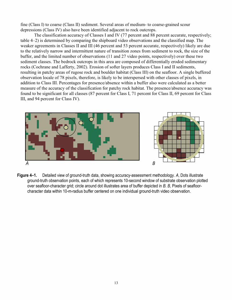
Next, circular buffer areas were created around individual observation points using a 10-m radius to account for layback and positional inaccuracies inherent to the towed-camera system. The radius length is an average of the distances between the positions of sharp interfaces seen on both the video (the position of the ship at the time of observation) and sonar data, plus the distance covered during a 10-second observation period at an average speed of 1 nautical mile/hour. Each buffer, which covers more than 300 m2, contains approximately 77 pixels. The classified (I, II, III) buffer is used as a mask to extract pixels from the seafloor-character map. These pixels are then compared to the class of the buffer. For example, if the shipboard-video observation is Class II (mixed smooth sediment and rock), but 12 of the 77 pixels within the buffer area are characterized as Class I (fine- to medium-grained smooth sediment), and 15 (of the 77) are characterized as Class III (rock and boulder, rugose), then the comparison would be “Class I, 12; Class II, 50; Class III, 15” (fig. 4–1). If the video observation of substrate is Class II, then the classification is accurate because the majority of seafloor pixels in the buffer are Class II. The accuracy values in table 4–2 represent the final of several classification iterations aimed at achieving the best accuracy, given the variable quality of sonar data (see discussion in Cochrane, 2008) and the limited ground-truth information available when compared to the continuous coverage provided by swath sonar. Presence/absence values in table 4–2 reflect the percentages of observations where the sediment classification of at least one pixel within the buffer zone agreed with the observed sediment type at a certain location.

The seafloor in the Offshore of Fort Ross map area is covered predominantly by Class I sediment composed of sand and mud. Several exposures of rugose bedrock (Class III) are present in the nearshore area between Fort Ross and Timber Cove. The rock outcrops are covered with varying thicknesses of

13

fine (Class I) to coarse (Class II) sediment. Several areas of medium- to coarse-grained scour depressions (Class IV) also have been identified adjacent to rock outcrops.

The classification accuracy of Classes I and IV (77 percent and 88 percent accurate, respectively; table 4–2) is determined by comparing the shipboard video observations and the classified map. The weaker agreements in Classes II and III (46 percent and 53 percent accurate, respectively) likely are due to the relatively narrow and intermittent nature of transition zones from sediment to rock, the size of the buffer, and the limited number of observations (11 and 27 video points, respectively) over these two sediment classes. The bedrock outcrops in this area are composed of differentially eroded sedimentary rocks (Cochrane and Lafferty, 2002). Erosion of softer layers produces Class I and II sediments, resulting in patchy areas of rugose rock and boulder habitat (Class III) on the seafloor. A single buffered observation locale of 78 pixels, therefore, is likely to be interspersed with other classes of pixels, in addition to Class III. Percentages for presence/absence within a buffer also were calculated as a better measure of the accuracy of the classification for patchy rock habitat. The presence/absence accuracy was found to be significant for all classes (87 percent for Class I, 71 percent for Class II, 69 percent for Class III, and 94 percent for Class IV).

Figure 4–1. Detailed view of ground-truth data, showing accuracy-assessment methodology. A, Dots illustrate ground-truth observation points, each of which represents 10-second window of substrate observation plotted over seafloor-character grid; circle around dot illustrates area of buffer depicted in B. B, Pixels of seafloor-character data within 10-m-radius buffer centered on one individual ground-truth video observation.

14

Table 4–1. Conversion table showing how video observations of primary substrate (more than 50 percent seafloor coverage), secondary substrate (more than 20 percent seafloor coverage), and abiotic seafloor complexity (in first three columns) are grouped into seafloor-character-map Classes I, II, III, and IV for use in supervised classification and accuracy assessment in Offshore of Fort Ross map area.

[In areas of low visibility where primary and secondary substrate could not be identified with confidence, recorded observations of substrate (in fourth column) were used to assess accuracy]

Primary-substrate component Secondary-substrate component Abiotic seafloor complexity Low-visibility observations

Class I mud mud low mud sand low sand mud low sand sand low sediment mud component ripples

Class II rock rock low sand boulders moderate sand rock low sand rock mod

Class III boulders boulders moderate boulders sand moderate rock boulders moderate rock rock moderate rock rock high rock sand moderate

Class IV sand sand low megaripples oscillatory megaripples depression

Table 4–2. Accuracy-assessment statistics for seafloor-character-map classifications in Offshore of Fort Ross map area.

[Accuracy assessments are based on video observations]

Class Number of observations % majority % presence/absence

I—Fine- to medium-grained smooth sediment 191 77.4 87.4

II—Mixed smooth sediment and rock 7 46.3 71.4

III—Rock and boulder, rugose 26 52.7 69.2

IV—Medium- to coarse-grained sediment (in scour depressions) 54 87.8 94.4

15

Chapter 5. Ground-Truth Studies for the Offshore of Fort Ross Map Area (Sheet 6) By Nadine E. Golden and Guy R. Cochrane

To validate the interpretations of sonar data in order to turn it into geologically and biologically useful information, the U.S. Geological Survey (USGS) towed a camera sled (fig. 5–1) over specific locations throughout the Offshore of Fort Ross map area to collect video and photographic data that would “ground truth” the seafloor. This ground-truth surveying occurred in 2008. The camera sled was towed 1 to 2 m above the seafloor, at speeds of between 1 and 2 nautical miles/hour. Ground-truth surveys in this map area include approximately 6 trackline kilometers of video and 524 still photographs, in addition to 346 recorded seafloor observations of abiotic and biotic attributes. A visual estimate of slope also was recorded.

Figure 5–1. Photograph of camera sled used in USGS 2008 ground-truth survey.

During the cruise, the USGS camera sled housed two standard-definition (640×480 pixel resolution) video cameras (one forward looking and one downward looking), a high-definition (1,080×1,920 pixel resolution) video camera, and an 8-megapixel digital still camera. During this cruise, in addition to recording the seafloor characteristics, a digital still photograph was captured once every 30 seconds.

The camera-sled tracklines (shown by colored dots on the map on sheet 6) are sited in order to visually inspect areas representative of the full range of bottom hardness and rugosity in the map area. The video is fed in real time to the research vessel, where USGS and National Oceanic and Atmospheric Administration (NOAA) scientists record both the geologic and biologic character of the seafloor. While the camera is deployed, several different observations are recorded for a 10-second period once every minute, using the protocol of Anderson and others (2007). Observations of primary substrate, secondary substrate, slope, abiotic complexity, biotic complexity, and biotic cover are mandatory. Observations of key geologic features and the presence of key species also are made.

Primary and secondary substrate, by definition, constitute greater than 50 and 20 percent of the seafloor, respectively, during an observation. The grain-size values that differentiate the substrate

16

classes are based on the Wentworth (1922) scale, and the sand, cobble, and boulder sizes are classified as in Wentworth (1922). However, the difficulty in distinguishing the finest divisions in the Wentworth (1922) scale during video observations made it necessary to aggregate some grain-size classes, as was done in the Anderson and others (2007) methodology: the granule and pebble sizes have been grouped together into a class called “gravel,” and the clay and silt sizes have been grouped together into a class called “mud.” In addition, hard bottom and clasts larger than boulder size are classified as “rock.” Benthic-habitat complexity, which is divided into abiotic (geologic) and biotic (biologic) components, refers to the visual classification of local geologic features and biota that potentially can provide refuge for both juvenile and adult forms of various species (Tissot and others, 2006).

Sheet 6 contains a smaller, simplified (depth-zone symbology has been removed) version of the seafloor-character map on sheet 5. On this simplified map, the camera-sled tracklines used to ground-truth-survey the sonar data are shown by aligned colored dots, each dot representing the location of a recorded observation. A combination of abiotic attributes (primary- and secondary-substrate compositions), as well as vertical variability, were used to derive the different classes represented on the seafloor-character map (sheet 5); on the simplified map, the derived classes are represented by colored dots. Also on this map are locations of the detailed views of seafloor character, shown by boxes (Boxes A through F); for each view, the box shows the locations (indicated by colored stars) of representative seafloor photographs. For each photograph, an explanation of the observed seafloor characteristics recorded by USGS and NOAA scientists is given. Note that individual photographs often show more substrate types than are reported as the primary and secondary substrate. Organisms, when present, are labeled on the photographs.

The ground-truth survey is designed to investigate areas that represent the full spectrum of high-resolution multibeam bathymetry and backscatter-intensity variation. Figure 5–2 shows that, in the Offshore of Fort Ross map area, the seafloor surface in water depths of less than about 50 m is predominately sand. Sediment sampling (Klise, 1983; Reid and others, 2006) indicates that the seafloor deeper than about 50 to 60 m is predominantly mud (see also, sheet 10). Nearshore rocky outcrops are present along the entire wave-exposed coast, locally more than 2 km offshore (see sheets 5, 10). Widespread areas of coarse sediment (fig. 4G on sheet 6) and scour depressions (figs. 3B, 5D on sheet 6) are found on the flanks of rocky outcrops, most of which are north of the mouth of the Russian River.

17

Figure 5–2. Graph showing distribution of primary and secondary substrate determined from video observations in Offshore of Fort Ross map area.

18

Chapter 6. Potential Marine Benthic Habitats of the Offshore of Fort Ross Map Area (Sheet 7) By H. Gary Greene, Charles A. Endris, and Bryan E. Dieter

The map on sheet 7 shows “potential” marine benthic habitats in the Offshore of Fort Ross map area, representing a substrate type, geomorphology, seafloor process, or any other attribute that may provide a habitat for a specific species or assemblage of organisms. This map, which is based largely on seafloor geology, also integrates information displayed on several other thematic maps of the Offshore of Fort Ross map area. High-resolution sonar bathymetry data, converted to depth grids (seafloor DEMs; sheet 1), are essential to development of the potential marine benthic habitat map, as is shaded-relief imagery (sheet 2), which allows visualization of seafloor terrain and provides a foundation for interpretation of submarine landforms.

Backscatter maps (sheet 3) also are essential for developing potential benthic habitat maps. High backscatter is further indication of “hard” bottom, consistent with interpretation as rock or coarse sediment. Low backscatter, indicative of a “soft” bottom, generally indicates a fine-sediment environment. Habitat interpretations also are informed by actual seafloor observations from ground-truth surveying (sheet 6), by seafloor-character maps that are based on video-supervised maximum-likelihood classification (sheet 5), and by seafloor-geology maps (sheet 10). The habitat interpretations on sheet 7 are further informed by the usSEABED bottom-sampling compilation of Reid and others (2006).

Broad, generally smooth areas of seafloor that lack sharp and angular edge characteristics are mapped as “sediment;” these areas may be further defined by various sedimentary features (for example, erosional scours and depressions) and (or) depositional features (for example, dunes, mounds, or sand waves). In contrast, many areas of seafloor bedrock exposures are identified by their common sharp edges and high relative relief; these may be contiguous outcrops, isolated parts of outcrop protruding through sediment cover (pinnacles or knobs), or isolated boulders. In many locations, areas within or around a rocky feature appear to be covered by a thin veneer of sediment; these areas are identified on the habitat map as “mixed” induration (that is, containing both rock and sediment). The combination of remotely observed data (for example, high-resolution bathymetry and backscatter, seismic-reflection profiles) and directly observed data (for example, camera transects, sediment samples) translates to higher confidence in the ability to interpret broad areas of the seafloor.

To avoid any possible misunderstanding of the term “habitat,” the term “potential habitat” (as defined by Greene and others, 2005) is used herein to describe a set of distinct seafloor conditions that in the future may qualify as an “actual habitat.” Once habitat associations of a species are determined, they can be used to create maps that depict actual habitats, which then need to be confirmed by in situ observations, video, and (or) photographic documentation.

Classifying Potential Marine Benthic Habitats Potential marine benthic habitats in the Offshore of Fort Ross map area are mapped using the

Benthic Marine Potential Habitat Classification Scheme, a mapping-attribute code developed by Greene and others (1999, 2007). This code, which has been used previously in other offshore California areas (see, for example, Greene and others, 2005, 2007), was developed to easily create categories of marine benthic habitats that can then be queried within a GIS or a database. The code contains several categories that can be subdivided relative to the spatial scale of the data. The following categories can be applied directly to habitat interpretations determined from remote-sensing imagery collected at a scale of tens of kilometers to one meter: Megahabitat, Seafloor Induration, Meso/Macrohabitat, Modifier, Seafloor Slope, Seafloor Complexity, and Geologic Unit. Additional categories of Macro/Microhabitat,

19

Seafloor Slope, Seafloor Complexity, and Geologic Attribute can be applied to habitat interpretations determined from seafloor samples, video, still photographs, or direct observations at a scale of 10 meters to a few centimeters. These two scale-dependent groups of categories can be used together, to define a habitat across spatial scales, or separately, to compare large- and small-scale habitat types.

The four categories and their attribute codes that are used on the Offshore of Fort Ross map area are explained in detail below (note, however, that not all categories may be used in a particular map area, given the study objectives, data availability, or data quality); attribute codes in each category are depicted on the map by the letters and, in some cases, numbers that make up the map-unit symbols:

Megahabitat—Based on depth and general physiographic boundaries; used to distinguish features on a scale of tens of kilometers to kilometers. Depicted on map by capital letter, listed first in map-unit symbol; generalized depth ranges are given below.

E = Estuary (0 to 100 m) S = Shelf; continental and island shelves (0 to 200 m) Seafloor Induration—Refers to substrate hardness. Depicted on map by lower-case letter, listed

second in map-unit symbol; may be further subdivided into distinct sediment types, depicted by lower-case letter(s) in parentheses, listed immediately after substrate hardness; multiple attributes listed in general order of relative abundance, separated by slash; queried where inferred.

h = Hard bottom (for example, rock outcrop or sediment pavement) m = Mixed hard and soft bottom (for example, local sediment cover of bedrock) s = Soft bottom; sediment cover (b) = Boulders (g) = Gravel (s) = Sand (m) = Mud, silt, and (or) clay Meso/Macrohabitat—Related to scale of habitat; consists of seafloor features one kilometer to

one meter in size. Depicted on map by lower-case letter and, in some cases, additional lower-case letter in parentheses, listed third in map-unit symbol; multiple attributes separated by slash.

b = Beach, relic (submerged) or shoreline (b)/p = Pinnacle indistinguishable from boulder d = Deformed, tilted and (or) folded bedrock; overhang e = Exposure; bedrock h = Hole; depression m = Mound; linear ridge p = Pinnacle; cone s = Scarp, cliff, fault, or slump scar w = Dynamic bedform y = Delta; fan Modifier—Describes texture, bedforms, biology, or lithology of seafloor. Depicted on map by

lower-case letter, in some cases followed by additional lower-case letter(s) either after hyphen or in parentheses (or both), following an underscore; multiple attributes separated by slash.

_a = Anthropogenic (artificial reef, breakwall, shipwreck, disturbance) _a-dg = Dredge groove or channel _a-g = Groin, jetty, rip-rap _a-w = Wreck, ship, barge, or plane

_c = Consolidated sediment (claystone, mudstone, siltstone, sandstone, breccia, or conglomerate)

_d = Differentially eroded _f = Fracture, joint; faulted

20

_g = Granite _h = Hummocky, irregular relief _r = Ripple (amplitude, greater than 10 cm) _s = Scour (current or ice; direction noted) _u = Unconsolidated sediment

Examples of Attribute Coding To illustrate how these attribute codes can be used to describe remotely sensed data, the

following examples are given: Ss(s)_u = Soft unconsolidated sediment (sand) on continental shelf. Es(s/m)_r/u = Rippled, soft, unconsolidated sediment (sand and mud) in estuary. She_g = Hard rock outcrop (granite), on continental shelf.

Map Area Habitats Delineated in the Offshore of Fort Ross map area are 13 potential marine benthic habitat types,

covering 117.10 km2 on the continental shelf (“Shelf” megahabitat). These include unconsolidated sediments (8 habitat types), mixed substrate (2 habitat types), and hard substrate (3 habitat types). The predominant habitat type is soft, unconsolidated sediment, which covers 107.26 km2 (91.6 percent) of the total area mapped. Exposed hard bedrock covers 8.53 km2 (7.3 percent), and sediment-covered bedrock, which is of the mixed hard-soft induration class, covers 1.31 km2 (1.1 percent). Rock outcrops and rubble are considered the primary habitat types for rockfish (Sebastes spp.) and lingcod (Ophiodon elongatus) (Cass and others, 1990; Love and others, 2002), both of which are recreationally and commercially important species.

21

Chapter 7. Subsurface Geology and Structure of the Offshore of Fort Ross Map Area and the Salt Point to Drakes Bay Region (Sheets 8 and 9) By Samuel Y. Johnson, Stephen R. Hartwell, and Janet T. Watt

The seismic-reflection profiles presented on sheet 8 provide a third dimension, depth, to complement the surficial seafloor-mapping data already presented (sheets 1 through 7) for the Offshore of Fort Ross map area. These data, which are collected at several resolutions, extend to varying depths in the subsurface, depending on the purpose and mode of data acquisition. The seismic-reflection profiles (sheet 8) provide information on sediment character, distribution, and thickness, as well as potential geologic hazards, including active faults, areas prone to strong ground motion, and tsunamigenic slope failures. The information on faults provides essential input to national and state earthquake-hazard maps and assessments (for example, Petersen and others, 2008).

The maps on sheet 9 show the following interpretations, which are based on the seismic-reflection profiles on sheet 8: the thickness of the uppermost sediment unit; the depth to base of this uppermost unit; and both the local and regional distribution of faults and earthquake epicenters (data from U.S. Geological Survey and California Geological Survey, 2010; Northern California Earthquake Data Center, 2014).

Data Acquisition Most profiles displayed on sheet 8 (figs. 1, 2, 3, 4, 6, 7, 9, 10, 11) were collected in 2009 on U.S.

Geological Survey (USGS) cruise S–8–09–NC. The single-channel seismic-reflection data were acquired using the SIG 2Mille minisparker that used a 500-J high-voltage electrical discharge fired 1 to 4 times per second, which, at normal survey speeds of 4 to 4.5 nautical miles/hour, gives a data trace every 0.5 to 2.0 m of lateral distance covered. The data were digitally recorded in standard SEG-Y 32-bit floating-point format, using Triton Subbottom Logger (SBL) software that merges seismic-reflection data with differential GPS-navigation data. After the survey, a short-window (20 ms) automatic gain control algorithm was applied to the data, along with a 160- to 1,200-Hz bandpass filter and a heave correction that uses an automatic seafloor-detection window (averaged over 30 m of lateral distance covered). These high-resolution data can resolve geologic features that are a few meters thick, down to subbottom depths of about 400 m.

Figures 5 and 8 on sheet 8 show deep-penetration, depth-migrated, multichannel seismic-reflection profiles collected in 1982 by WesternGeco on cruise W–4–82–NC. These profiles and other similar data were collected in many areas offshore of California in the 1970s and 1980s when these areas were considered a frontier for oil and gas exploration. Most of these data have been publicly released and are now archived at the U.S. Geological Survey National Archive of Marine Seismic Surveys (U.S. Geological Survey, 2009). These data were acquired using a large-volume air-gun source that has a frequency range of 3 to 40 Hz and recorded with a multichannel hydrophone streamer about 2 km long. Shot spacing was about 30 m. These data can resolve geologic features that are 20 to 30 m thick, down to subbottom depths of about 4 km.

Seismic-Reflection Imaging of the Continental Shelf Sheet 8 shows seismic-reflection profiles in the Offshore of Fort Ross map area. The north half

of the map area is characterized by nearshore rocky outcrops. The nearshore zone and inner shelf area (to water depths of about 50 m) typically dip gently seaward (about 1.5° to 2.5°), whereas the midshelf

22

area (about 50 to 85 m) is relatively flat (about 0.4°). In contrast, the nearshore to midshelf area in the south half of the map area have a more uniform dip (about 0.45° to 0.8°), out to water depths of about 70 m. The south half of the map area lies directly offshore of the mouth of the Russian River, and this southward decrease in slope is caused by increased sedimentation and sediment thickness (Map B on sheet 9) in this deltaic setting.

Shallow-marine and shelf sediments were deposited in the last about 21,000 years during the sea-level rise that followed the last major lowstand associated with the Last Glacial Maximum (LGM) (Fairbanks, 1989; Fleming and others, 1998; Lambeck and Chappell, 2001; Peltier and Fairbanks, 2006). Sea level was about 125 m lower during the LGM, at which time the Offshore of Fort Ross map area was emergent, and the shoreline was about 20 km west of its present location. The post-LGM sea-level rise was rapid (about 9 to 11 m per thousand years) until about 7,000 years ago, when it slowed considerably to about 1 m per thousand years (Peltier and Fairbanks, 2006; Stanford and others, 2011). Sea-level rise led to broadening of the continental shelf, progressive eastward migration of the shoreline and wave-cut platform, and associated transgressive erosion and deposition (see, for example, Catuneanu, 2006).

The sediments deposited during the post-LGM sea-level rise (the rapid transgression and highstand) are shaded blue in the high-resolution seismic-reflection profiles on sheet 8 (figs. 1, 2, 3, 4, 6, 7, 9, 10, 11), and their thickness is shown on sheet 9 (Maps B, D). Sediment supply is almost entirely from the mouth of the Russian River. This post-LGM stratigraphic unit is characterized by relatively low-amplitude, low- to high-frequency, parallel to divergent reflections that typically are continuous to moderately continuous (terminology from Mitchum and others, 1977). The relatively low amplitude can be caused by extensive winnowing from wave energy and currents, resulting in a uniform sediment grain size. These conditions tend to minimize the acoustic-impedance contrasts needed to produce seismic reflections that have higher amplitudes. The contact between these sediments and the underlying strata is an abrupt transgressive erosional surface (see, for example, Catuneanu, 2006), which commonly is marked by minor channeling, an upward change to lower amplitude, more diffuse reflections, and eastward onlap on reflection-free (that is, massive) bedrock.

Strata beneath the post-LGM unit (which overlie the Tertiary basement rocks) are represented on sheet 8 (figs. 1, 2, 3, 4, 6, 7, 9, 10, 11) by low- to high-amplitude, high-frequency, parallel to subparallel, continuous reflections. Reflections commonly are flat to gently folded and typically have dips of 0° to 2° to a maximum (in the northern part of the map area) of about 5° (note that dips may appear steeper on the profiles because of the 12.5:1 vertical exaggeration). The upper contact with the post-LGM unit ranges from angular (where the lower unit has been folded) to parallel or subparallel. These strata are inferred to be Pleistocene in age (marine isotope stage 3 and older; Wright, 2000; Waelbroeck and others, 2002) because they underlie post-LGM strata; in addition, their horizons can be traced continuously, along with other USGS data (from cruise S–8–09–NC), to the Quaternary section penetrated by Shell Oil Company offshore well P–027–1 (15 km south of the map area; Heck and others, 1990). Similar to the overlying post-LGM deposits, these inferred Pleistocene strata are wave-reworked deltaic and shelf sediments derived primarily from the Russian River. Reflections within this interval are locally obscured by interstitial gas within the sediment (see, for example, figs. 1, 2, 3, 4, 11 on sheet 8). This effect has been referred to as “gas blanking,” “acoustic turbidity,” or “acoustic masking” (Hovland and Judd, 1988; Fader, 1997). The gas scatters or attenuates the acoustic energy from the seismic-reflection-profiling system, inhibiting penetration of strata.

The map area is cut by the San Andreas Fault (figs. 4, 6, 7, 9, 10, 11 on sheet 8). West of the San Andreas Fault, bedrock exposed along the coast (onshore and offshore) consists of the Paleocene and Eocene German Rancho Formation (Elder, 1998; Wentworth and others, 1998) and the lower Miocene sandstone and mudstone of Fort Ross area (see sheet 10; see also, Blake and others, 2002). East of the San Andreas Fault, coastal bedrock outcrops consist of the Jurassic and (or) Cretaceous mélange of the

23

Franciscan Complex and the Cretaceous Great Valley sequence conglomerate of Healdsburg terrane. These bedrock units are cut by numerous small faults, and steep dips are common in coastal outcrops. These units appear massive and reflection free on high-resolution seismic-reflection profiles (see, for example, figs. 2, 4, 6, 7, 9 on sheet 8), and they form the acoustic basement for overlying Quaternary sediments. On the higher energy, lower resolution seismic profiles (figs. 5, 8), bedrock west of the San Andreas Fault (inferred to be Tertiary sedimentary rocks) is characterized by low- to high-amplitude, parallel to divergent, continuous reflections.

Geologic Structure and Recent Deformation The Offshore of Fort Ross map area is cut by the northwest-striking San Andreas Fault Zone

(fig. 1–1), the right-lateral transform boundary between the North American and Pacific plates. North of Fort Ross, the San Andreas Fault forms a prominent topographic lineament in low coastal hills. Geologic studies in the onshore area suggest a slip rate of 17 to 24 mm/yr (U.S. Geological Survey and California Geological Survey, 2010). South of Fort Ross, the San Andreas Fault extends across the wave-dominated Russian River delta. The San Andreas Fault and other faults are identified on seismic-reflection profiles (sheet 8) on the basis of the abrupt truncation or warping of reflections and (or) the juxtaposition of reflection panels that have differing seismic parameters, such as reflection presence, amplitude, frequency, geometry, continuity, and vertical sequence. The mapping reveals a 200- to 500-m-wide zone typically characterized by one or two primary fault strands (see sheet 10).

Sheet 8 shows six profiles that transect the San Andreas Fault (figs. 4, 6, 7, 9, 10, 11), which illustrate the complex geology within the fault zone. The northernmost three of these six profiles (figs. 4, 6, 7) show prominent, asymmetric, intra–fault-zone basins (about 15 to 25 m deep) filled with post-LGM sediment. In contrast, two of the other profiles across the San Andreas Fault Zone (figs. 9, 10), both of which are less than 2 km south of the profile shown in figure 7, reveal minor uplift between the two primary fault strands within the zone. Such transitions probably are the result of gentle fault bends and transfers of slip between subparallel faults (see sheet 10; see also, for example, Mann, 2007; Johnson and Watt, 2012).

Geologic structure west of the San Andreas Fault in most of the Offshore of Fort Ross map area is relatively simple. The bedrock surface dips offshore about 1° to 2°, and it is overlain by an eastward- and southward-thinning wedge of flat-lying reflections of inferred late Pleistocene age.

McCulloch (1987) mapped a northwest-striking fault zone in the nearshore (within 3 to 5 km of the shoreline) that extends from Point Arena to Fort Ross, using deep-penetration industry seismic-reflection data; Dickinson and others (2005) named this structure the “Gualala Fault.” On sheet 8 (fig. 5), this structure is imaged as a steep, northeast-striking fault. Other profiles on sheet 8 show the fault as ending to the southeast in the offshore between Fort Ross and the mouth of the Russian River; for example, figure 8, which crosses the strike of this structure, shows more than 1 km of undisturbed parallel reflections. Coincidence of the deeper parts of the Gualala Fault with a zone of shallow folding (see, for example, fig. 1) and faulting (seen on high-resolution seismic profiles collected north of the map area, on USGS cruise S–8–09–NC) suggests that the Gualala Fault was active as a blind structure in the late Quaternary.

Map E on sheet 9 shows the regional pattern of major faults and earthquakes. Fault locations, which have been simplified, are compiled from our mapping within California’s State Waters (see sheet 10) and from the U.S. Geological Survey’s Quaternary fault and fold database (U.S. Geological Survey and California Geological Survey, 2010). Earthquake epicenters are from the Northern California Earthquake Data Center (2014), which is maintained by the U.S. Geological Survey and the University of California, Berkeley, Seismological Laboratory; all events of magnitude 2.0 and greater for the time period 1967 through March 2014 are shown. The largest recorded earthquake in the map area (M2.6,

24

5/18/2003) was located west of Fort Ross, within the deformation zone associated with the Gualala Fault. A notable lack of microseismicity on the adjacent San Andreas Fault has occurred since the devastating great 1906 California earthquake (M7.8, 4/18/1906), thought to have nucleated on the San Andreas Fault offshore of San Francisco (see, for example, Bolt, 1968; Lomax, 2005), about 90 km south of the map area.

Thickness and Depth to Base of Uppermost Pleistocene and Holocene Deposits Maps on sheet 9 show the thickness and the depth to base of uppermost Pleistocene and

Holocene (post-LGM) deposits both for the Offshore of Fort Ross map area (Maps A, B) and, to establish regional context, for a larger area (about 115 km of coast) that extends from the Salt Point area south to the southern part of the Point Reyes peninsula (Maps C, D). To make these maps, water bottom and depth to base of the LGM horizons were mapped from seismic-reflection profiles using Seisworks software. The difference between the two horizons was exported from Seisworks for every shot point as XY coordinates (UTM zone 10) and two-way travel time (TWT). The thickness of the post-LGM unit (Maps B, D) was determined by applying a sound velocity of 1,600 m/sec to the TWT, resulting in thicknesses as great as about 56 m. The thickness points were interpolated to a preliminary continuous surface, overlaid with zero-thickness bedrock outcrops (see sheet 10), and contoured following the methodology of Wong and others (2012).

Several factors required manual editing of the preliminary sediment-thickness maps to make the final product. The Gualala, Point Reyes, and San Andreas Faults disrupt the sediment sequence in the region (Maps D, E on sheet 9). The thickness data points also are dense along tracklines (about 1 m apart) and sparse between tracklines (1 km apart), resulting in contouring artifacts. To incorporate the effect of the faults, to remove irregularities from interpolation, and to reflect other geologic information and complexity, the resulting interpolated contours were modified. Contour modifications and regridding were repeated several times to produce the final regional sediment-thickness map (Wong and others, 2012). Information for the depth to base of the post-LGM unit (Maps A, C on sheet 9) was generated by adding the thickness data to water depths determined by multibeam bathymetry (see sheet 1).

The thickness of the post-LGM unit in the Offshore of Fort Ross map area ranges from 0 to 56 m (Map B on sheet 9), and the depth to the base of this unit reaches a maximum of about 100 m (Map A on sheet 9). Mean sediment thickness for the map area is 20.8 m, and the total sediment volume is 2,393×106 m3 (table 7–1). The thickest sediment in the map area, and within the larger Salt Point to Drakes Bay region (Maps B, D), is found in narrow, elongate, fault-bounded basins within the San Andreas Fault Zone. Apart from these small tectonic basins, the thickest (as much as 41 m) uppermost Pleistocene and Holocene sediment in the Offshore of Fort Ross map area (Map B) and in the broader region (Map D) is found offshore of the mouth of the Russian River, at water depths of about 30 to 60 m. The Russian River has a very large sediment load (estimated 900,000 metric tons/yr; Farnsworth and Warrick, 2007), and the greater sediment thickness in this midshelf area is tied to this source. Sediment thickness diminishes to the northwest in an area of fine-grained sediment, or “mud belt,” that also is derived from the Russian River (Klise, 1983; Drake and Cacchione, 1985).

In the northern nearshore zone from near Timber Gulch to the northwest corner of the map area (Maps A, B), bedrock forms seafloor outcrops that extend out from the shoreline between 500 and 2,500 m, to water depths of about 50 m. In a few places at the mouths of coastal watersheds (for example, Timber Cove Creek; fig. 1–2), lowstand fluvial channels have been eroded into the nearshore bedrock then subsequently filled with sediment. In the southern nearshore zone, northeast of the offshore San Andreas Fault, the shallow areas (depths of 0 to 15 m) that are within about 1 km of the shoreline are characterized by less continuous rocky outcrop and thin sediment cover.

25

Five different “domains” of sediment thickness are recognized on the regional sediment-thickness map (Map D on sheet 9), each with distinctive geologic controls: (1) The Salt Point shelf domain, located in the far northwestern part of the region, has a mean sediment thickness of 11.7 m. The thickest sediment (20 to 25 m) is found where a pre-LGM, regressive, downlapping sediment wedge formed above a break in slope that is controlled by a contact between harder bedrock and softer, folded Pleistocene strata. Sediment thinning in this domain within the outer parts of California’s State Waters is the result of a relative lack of sediment supply from local watersheds, as well as a more distal Russian River source. (2) The Russian River delta and mud belt domain, located offshore of the Russian River, the largest sediment source on this part of the coast, has the thickest uppermost Pleistocene and Holocene sediment in the region (mean thickness, 21.1 m). The northward extension into the midshelf “mud belt” results from northward shelf-bottom currents and sediment transport (Drake and Cacchione, 1985). This domain includes a section of the San Andreas Fault Zone, which here is characterized by several releasing, right-stepping strands that bound narrow, elongate pull-apart basins; these sedimentary basins contain the greatest thickness of uppermost Pleistocene and Holocene sediment (about 56 m) in the region. (3) The Bodega Head–Tomales Point shelf domain, located between Bodega Head and the Point Reyes headland, contains the least amount of sediment in the region (mean thickness, 3.4 m). The lack of sediment primarily reflects decreased accommodation space and limited sediment supply. (4) The Point Reyes bar domain, located west and south of the Point Reyes headland, is a local zone of increased sediment thickness (mean thickness, 14.3 m) created by bar deposition on the more protected south flank of the Point Reyes headland during rising sea level. (5) The Bolinas shelf domain, located east and southeast of the Point Reyes headland, has a thin sediment cover (mean thickness, 5.6 m), which likely results from limited sediment accommodation space caused by tectonic uplift (water depths in this domain within California’s State Waters are less than 45 m), and high wave energy, capable of reworking and transporting shelf sediment to deeper water.

Table 7–1. Area, sediment-thickness, and sediment-volume data for California’s State Waters in Salt Point to Drakes Bay region (domains 1–5), as well as in Offshore of Fort Ross map area.

Regional sediment-thickness domains in Salt Point to Drakes Bay region

Area (km2) Mean sediment thickness (m)

Sediment volume (106 m3)

Entire Salt Point to Drakes Bay region 714 9.5 6,794

(1) Salt Point shelf 90 11.7 1,054

(2) Russian River delta and mud belt 144 21.1 3,031

(3) Bodega Head–Tomales Point shelf 275 3.4 928

(4) Point Reyes bar 72 14.3 1,029

(5) Bolinas shelf 133 5.6 752

Sediment thickness in Offshore of Fort Ross map area

Entire Offshore of Fort Ross map area 115 20.8 2,393

26

Chapter 8. Geologic and Geomorphic Map of the Offshore of Fort Ross Map Area (Sheet 10) By Samuel Y. Johnson, Michael W. Manson, and Stephen R. Hartwell

Geologic and Geomorphic Summary Marine geology and geomorphology were mapped in the Offshore of Fort Ross map area from

approximate Mean High Water (MHW) to the 3-nautical-mile limit of California’s State Waters. MHW is defined at an elevation of 1.46 m above the North American Vertical Datum of 1988 (NAVD 88) (Weber and others, 2005). Offshore geologic units were delineated on the basis of integrated analyses of adjacent onshore geology with multibeam bathymetry and backscatter imagery (sheets 1, 2, 3), seafloor-sediment and rock samples (Reid and others, 2006), digital camera and video imagery (sheet 6), and high-resolution seismic-reflection profiles (sheet 8). Aerial photographs taken in multiple years were used to map the nearshore area (0 to 10 m water depth) and to link the offshore and onshore geology. The relative proportions of all offshore map units are shown in table 8–1.

Onshore bedrock units are compiled from Huffman (1972), Blake and others (2002), Manson and others (2006), and Wagner and Gutierrez (2010), as well as unpublished mapping in the Bodega Bay 30′ × 60′ quadrangle by D.L. Wagner and C.I. Gutierrez, California Geological Survey; in addition, some Franciscan Complex units are modified from previously unpublished mapping (E.H. Bailey, W.P. Irwin, U.S. Geological Survey; D.L. Wagner, M.W. Manson, California Geological Survey); unit ages, which are derived from these sources, reflect local stratigraphic relations. Onshore Quaternary units are compiled from Witter and others (2006), with some additional mapping by M.W. Manson (this report); in addition, some units are modified by M.W. Manson on the basis of analysis of 2003 lidar and 2004 ifsar imagery. Traces of the San Andreas Fault are compiled from California Geological Survey (1974a,b,c) and previously unpublished mapping by M.W. Manson.

The geomorphology and geology of the offshore part of the map area result from the interplay between local sedimentary processes, oceanography, sea-level change, and tectonics. The seafloor in the north half of the map area is characterized by rocky outcrops of Tertiary sedimentary rocks (units Tgr and Tsm). The rugged nearshore zone and the inner shelf area (to water depths of about 50 m) typically dip seaward (about 1.5° to 2.5°), whereas the midshelf area within California’s State Waters (about 50 to 85 m deep) dips more gently (about 0.4°). In contrast, the nearshore to midshelf area in the south half of the map area, which lies directly offshore of the mouth of the Russian River, has a more uniform dip: about 0.45° out to water depths of about 30 m and about 0.65° to 0.8° at water depths of between 30 and 70 m. A substantial amount of the Russian River sediment load, which is estimated to be about 900,000 metric tons/yr (Farnsworth and Warrick, 2007), is deposited offshore of the river mouth (see Map B on sheet 9), contributing to the north-to-south contrast in bathymetric slope. On a larger geomorphic scale, sea level has risen about 125 m over the last about 21,000 years (see, for example, Lambeck and Chappell, 2001; Peltier and Fairbanks, 2006), leading to broadening of the continental shelf, progressive eastward migration of the shoreline and wave-cut platform, and associated transgressive erosion and deposition. Tectonic influences on the geomorphology and geology of the shelf are related primarily to the active San Andreas Fault system.

Given the exposure to high wave energy, the modern nearshore to inner shelf sediments north of the mouth of the Russian River are mostly sand (unit Qms) and a mix of sand, gravel, and cobbles (units Qmsc and Qmsd). Coarser grained sands and gravels (units Qmsc and Qmsd) are recognized primarily on the basis of bathymetry and high backscatter (sheets 1, 2, 3). Both units Qmsc and Qmsd typically have abrupt landward contacts with bedrock (units Tgr, Tsm, TKfs, fsr), and they form

27

irregular to lenticular exposures that commonly are elongate perpendicular to the shoreline. Contacts between units Qmsc and Qms are generally gradational.

Unit Qmsd typically forms erosional lags in scour depressions that are bounded by relatively sharp or, less commonly, diffuse contacts with the horizontal sand sheets of unit Qms. These depressions generally are a few tens of centimeters deep and range in size from a few tens of square meters to more than 1 km2. Such scour depressions are common along this stretch of the California coast (see, for example, Cacchione and others, 1984; Hallenbeck and others, 2012) where offshore sandy sediment can be relatively thin (and, thus, is unable to fill the depressions) owing to lack of sediment supply from rivers and also to significant erosion and offshore transport of sediment during large northwest winter swells. Such features have been referred to as “rippled scour depressions” (see, for example, Cacchione and others, 1984) or “sorted bedforms” (see, for example, Goff and others, 2005; Trembanis and Hume, 2011). Although the general areas in which both unit Qmsd scour depressions and surrounding Qms sand sheets are found are not likely to change substantially, the boundaries of the unit(s) likely are ephemeral, changing seasonally and during significant storm events.

Unit Qmsf, which lies offshore of unit Qms, consists primarily of mud and muddy sand, and it commonly is extensively bioturbated. The water depth of the transition from sand-dominated marine sediment (unit Qms) to mud-dominated marine sediment (unit Qmsf) increases from about 45 to 50 m directly offshore of the mouth of the Russian River to as much as about 60 m adjacent to the rocky outcrops near the north edge of the map area. This change probably is related to the large amount of fine-sediment load carried by the Russian River, which feeds a widespread midshelf mud belt that extends from Point Arena to Point Reyes (fig. 1–1) (Klise, 1983; Drake and Cacchione, 1985; Demirpolat, 1991).

The Offshore of Fort Ross map area is cut by the northwest-striking San Andreas Fault, the right-lateral transform boundary between the North American and Pacific plates. The San Andreas Fault extends across the inner shelf in the southern part of the map area, then it crosses the shoreline at Timber Gulch (fig. 1–2) and continues onland for about 75 km to the east flank of Point Arena (fig. 1–1) (Lawson, 1908; Brown and Wolfe, 1972). Seismic-reflection data (see sheet 8) are used to map the offshore fault trace, and they reveal a 200- to 500-m-wide fault zone that typically is characterized by one or two primary fault strands. In the southern part of the map area, about 1,500 m west of the San Andreas Fault, the midshelf (water depths of between 40 and 70 m) area includes an about 5-km-wide field of elongate pairs of sediment lobes and chutes (unit Qmsl) oriented perpendicular to slope. Individual lobes within the field, which are as much as 650 m long and 200 m wide, have as much as 2.5 m of relief above the surrounding seafloor, and they typically are transitional to the upslope chutes. Given their morphology and their proximity to the San Andreas Fault, we infer that these lobes result from offshore slope failures associated with strong ground motions triggered by large earthquakes on the San Andreas Fault.

Movement on the San Andreas Fault has juxtaposed coastal-bedrock blocks of different ages and lithologies (Blake and others, 2002). Bedrock northeast of the fault, found along the coast and in the nearshore, is mapped as the Jurassic, Cretaceous, Paleocene, and (or) Eocene rocks of the Franciscan Complex, either the sandstone within Coastal or Central Belt (unit TKfs) or the mélange in Central Belt (unit fsr). Bedrock southwest of the fault is considered to be part of the Gualala block (Elder, 1998), and it includes rocks of the Paleocene and Eocene German Rancho Formation (unit Tgr) and the Miocene sandstone and mudstone of Fort Ross area (unit Tsm).

The onshore section of the San Andreas Fault has an estimated slip rate of about 17 to 24 mm/yr (U.S. Geological Survey and California Geological Survey, 2010). The devastating great 1906 California earthquake (M7.8) is thought to have nucleated on the San Andreas Fault about 90 kilometers south of the map area, offshore of San Francisco (see, for example, Bolt, 1968; Lomax, 2005), the rupture extending northward through the Offshore of Fort Ross map area to the south flank of Cape

28

Mendocino. Emergent marine terraces along the coast in the Offshore of Fort Ross map area record recent contractional deformation and uplift associated with the San Andreas Fault system. Uplift rates of 0.3 to 0.6 mm/yr were reported by Prentice and Kelson (2006) for a late Pleistocene terrace exposed at Fort Ross, and this recent uplift also must have affected the adjacent nearshore and inner shelf areas.

McCulloch (1987) mapped a fault zone in the nearshore (within 3 to 5 km of the shoreline) that extends from Point Arena to Fort Ross (fig. 1–1), primarily using deep-penetration industry seismic-reflection data; Dickinson and others (2005) named this structure the “Gualala Fault.” Our mapping, also based on seismic-reflection data (see sheet 8), reveals this structure to be a steep, northeast striking fault whose southeast termination is in the offshore between Fort Ross and the mouth of the Russian River. We have designated the zone of shallow faulting and folding associated with this structure as the “Gualala Fault deformation zone.”

Table 8–1. Areas and relative proportions of offshore geologic map units in Offshore of Fort Ross map area. Map Unit Area (m2) Area (km2) Percent of total area

Marine sedimentary units Qms 44,541,413 44.5 35.6

Qmsc 3,910,887 3.9 3.1

Qmsf 47,934,012 47.9 38.3

Qmsd 7,189,417 7.2 5.8

Qmsl 5,380,590 5.4 4.3

Total, sedimentary units 108,956,319 109.0 87.1

Marine bedrock and (or) shallow bedrock units Tsm 6,158,599 6.2 4.9

Tgr 5,486,126 5.5 4.4

TKfs 818,720 0.8 0.7

fsr 3,604,113 3.6 2.9

Total, bedrock units 16,067,558 16.1 12.9

Total, Offshore of Fort Ross map area 125,023,877 125.0 100.0

29

DESCRIPTION OF MAP UNITS

OFFSHORE GEOLOGIC AND GEOMORPHIC UNITS Qms Marine nearshore and shelf deposits (late Holocene)—Predominantly sand; ripple marks

common; found on gently seaward-dipping (less than 2°) surface that extends from shoreline to depths of about 25 to 30 m offshore of Russian River and also to depths of as much as 50 to 60 m in northern part of map area

Qmsc Coarse-grained marine nearshore and shelf deposits (late Holocene)—Predominantly coarse sand, gravel, and cobbles; found on gently seaward-dipping (less than 2°) surface, at depths typically less than about 50 m; recognized primarily on basis of high backscatter and flat relief

Qmsf Fine-grained marine shelf deposits (late Holocene)—Predominantly mud and muddy sand; commonly bioturbated; found on gently seaward-dipping (less than 1°) surface, at depths greater than about 25 to 30 m offshore of mouth of Russian River and also at depths of more than 50 to 60 m in northern part of map area

Qmsd Marine shelf scour depressions (late Holocene)—Inferred to be coarse sand and possibly gravel; consists of irregular, arcuate scour depressions that vary from solitary features occupying a few hundred square meters to fields of interconnected depressions covering tens of thousands of square meters. Backscatter data and camera observations show intensity contrasts that suggest depressions are filled with sediment that is coarser than intervening elevated sandy shelf deposits (unit Qms). Depressions typically are 15 to 50 cm deep, and they have diffuse boundaries on shoreward edge that grade to sharp, well-defined boundaries on offshore, distal edge. General area in which unit is found is not likely to change substantially, but boundaries of unit(s) and locations of individual depressions (and intervening flat sheets) likely are ephemeral, changing during significant storm events

Qmsl Marine midshelf sediment lobes (late Holocene)—Fields of elongate, shore-normal pairs of sediment lobes (inferred to consist of mixture of sand and mud) and chutes, at depths of between 40 and 70 m in southern part of map area; individual lobes are as much as 650 m long and 200 m wide, and they have as much as 2.5 m of relief above surrounding smooth seafloor

Tsm Sandstone and mudstone of Fort Ross area (Blake and others, 2002) (early Miocene)—Grayish-white arkose overlain by black, fissile, clayey siltstone; sandstone interbedded with black mudstone

Tgr German Rancho Formation (Elder, 1998) (Eocene and Paleocene)—Well-bedded, fine- to medium-grained sandstone, mudstone, and conglomerate

Franciscan Complex TKfs Sandstone within Coastal or Central Belt (late Eocene to Late Cretaceous)—Mostly

massive, feldspathic-lithic wacke fsr Mélange in Central Belt (Cretaceous and (or) Jurassic)—Matrix of sheared argillite,

graywacke, and minor green tuff that encloses blocks and lenses of graywacke, chert, metachert, greenstone, serpentinite, silica-carbonate rock, blueschist (metasediment and metabasalt), eclogite, amphibolite, limestone, and quartz-mica schist (Blake and others, 2002)

30

ONSHORE GEOLOGIC AND GEOMORPHIC UNITS

[Bedrock units compiled from Huffman (1972), Blake and others (2002), Manson and others (2006), and Wagner and Gutierrez (2010), as well as previously unpublished mapping; unit ages, which are from these sources, reflect local stratigraphic relations. Quaternary units compiled from Witter and others (2006), with some additional mapping by M.W. Manson (this report); in addition, some units modified by M.W. Manson on basis of interpretation of 2003 lidar and 2004 ifsar imagery]

af Artificial fill (late Holocene)—Material deposited by humans alf Artificial groin (late Holocene)—Groin constructed at mouth of Russian River Qsc Stream-channel deposits (late Holocene)—Fluvial deposits within active, natural stream

channels Qbs Beach-sand deposits (late Holocene)—Active beaches in coastal environments; may form

veneer over bedrock platform Qt Stream-terrace deposits (late Holocene)—Stream-terrace deposits judged to be latest

Holocene age (<1,000 years) on basis of records of historical inundation and (or) identification of youthful meander scars and braid bars on aerial photographs or lidar imagery

Qf Alluvial fan deposits (Holocene)—Sediment deposited by streams emanating from mountain canyons onto alluvial valley floors or alluvial plains; may include debris-flow, hyperconcentrated-mudflow, and braided-stream deposits

Qa Alluvial deposits, undivided (Holocene)—Alluvium deposited in fan, terrace, or basin environments

Qoa Alluvial deposits, undivided (Holocene and late Pleistocene)—Mapped in small valleys where separate fan, basin, and terrace units could not be delineated at map scale and also where deposits might be of either late Pleistocene or Holocene age

Qls Landslide deposits (Holocene and Pleistocene)—Weathered rocks and soil; ranges from deep-seated landslides to active colluvium. Internal contacts differentiate individual landslide bodies

Qmt Marine-terrace deposits (late Pleistocene)—Sand, gravel, and cobbles; deposited on marine-abrasion platforms and later uplifted to present-day elevations along coast

Tor Ohlson Ranch Formation (Blake and others, 2002) (Pliocene)—Horizontal, thickly bedded, well-consolidated sandstone

Tb Basalt of Fort Ross (Miocene?)—Basalt that forms two small knobs near Fort Ross; surrounded by marine-terrace deposits; bedrock contacts not exposed

Tsm Sandstone and mudstone of Fort Ross area (Blake and others, 2002) (early Miocene)—Grayish-white arkose overlain by black, fissile, clayey siltstone; sandstone interbedded with black mudstone

Tgr German Rancho Formation (Elder, 1998) (Eocene and Paleocene)—Well-bedded, fine- to medium-grained sandstone, mudstone and conglomerate

TKu German Rancho and Gualala Formations, undivided (Elder, 1998) (Eocene, Paleocene, and Late Cretaceous)—Sandstone, conglomerate, mudstone, and shale

Kgv Great Valley sequence conglomerate of Healdsburg terrane (Cretaceous)—Pebble to boulder conglomerate

Franciscan Complex (Eocene, Paleocene, Cretaceous, and Jurassic) TKfs Sandstone in Coastal or Central Belt (late Eocene to Late Cretaceous)—Mostly

massive, feldspathic-lithic wacke; locally includes thin beds of sandstone and dark-gray shale and slate; lacks known fossils or other stratigraphic control (Blake and others, 2002)

31

Kfs Sandstone in Central Belt (Cretaceous)—Massive to distinctively bedded, feldspathic and feldspathic-lithic wacke

KJfmb Metabasalt in Eastern Belt (Cretaceous and (or) Jurassic)—Blueschist-facies metabasalt (Blake and others, 2002)

KJfsch Metamorphic rocks in Eastern Belt (Cretaceous and (or) Jurassic)—Variably sheared tectonic mixture of metamorphic rocks that contain blueschist; predominantly metagraywacke that has weak to moderate foliation, as well as metashale and metagreenstone; tectonic inclusions of coarse-grained metamorphic rocks and metachert are common

fsr Mélange in Central Belt (Cretaceous and (or) Jurassic)—Matrix of sheared argillite, graywacke, and minor green tuff that encloses blocks and lenses of graywacke, chert, metachert, greenstone, serpentinite, silica-carbonate rock, blueschist (metasediment and metabasalt), eclogite, amphibolite, limestone, and quartz-mica schist (Blake and others, 2002)

gwy Graywacke and metagraywacke blocks within mélange (Cretaceous and (or) Jurassic)

ch Chert and metachert blocks within mélange (Cretaceous and (or) Jurassic)—Includes massive and thinly bedded red, green, and white chert and metachert

gs Greenstone blocks within mélange (Cretaceous and (or) Jurassic)—Includes massive and pillowed greenstone and basalt

sch Schist and semischist blocks within mélange (Cretaceous and (or) Jurassic) sp Ultramafic rocks in Central Belt (Cretaceous and (or) Jurassic)—Partly to

completely serpentinized peridotite

32

Acknowledgments This publication was funded by the California Ocean Protection Council and the U.S. Geological

Survey (USGS) Coastal and Marine Geology Program. We thank the officers, crew, and scientific parties of the ships—R/V VenTresca, California State University, Monterey Bay, Seafloor Mapping Lab; and F/V Quicksilver, Fugro Pelagos—for their skill and professionalism in collecting the data presented in this report. We thank Daniel Brothers, Steve Watt, and Scott Starratt (all USGS) for their critical reviews that greatly improved this report. We are very grateful to USGS editor Taryn Lindquist for helping us develop the templates and formats for this series of publications, and for invaluable editorial review and suggestions.

33

References Cited Anderson, T.J., Cochrane, G.R., Roberts, D.A., Chezar, H., and Hatcher, G., 2007, A rapid method to

characterize seabed habitats and associated macro-organisms, in Todd, B.J., and Greene, H.G., eds., Mapping the seafloor for habitat characterization: Geological Association of Canada Special Paper 47, p. 71–79.

Blake, M.C., Jr., Graymer, R.W., and Stamski, R.E., 2002, Geologic map and map database of western Sonoma, northernmost Marin, and southernmost Mendocino Counties, California: U.S. Geological Survey Miscellaneous Field Studies Map 2402, scale 1:100,000, available at http://pubs.usgs.gov/mf/ 2002/2402/.

Bolt, B.A., 1968, The focus of the 1906 California earthquake: Bulletin of the Seismological Society of America, v. 58, p. 457–471.

Brown, R.D., Jr., and Wolfe, E.W., 1972, Map showing recently active breaks along the San Andreas Fault between Point Delgada and Bolinas Bay, California: U.S. Geological Survey Miscellaneous Investigations Map I–692, scale 1:24,000.

Cacchione, D.A., Drake, D.E., Grant, W.D., and Tate, G.B., 1984, Rippled scour depressions of the inner continental shelf off central California: Journal of Sedimentary Petrology, v. 54, p. 1,280–1,291.

California Department of Fish and Wildlife, 2008, California Marine Life Protection Act master plan for marine protected areas—Revised draft: California Department of Fish and Wildlife [formerly California Department of Fish and Game], available at http://www.dfg.ca.gov/mlpa/masterplan.asp.

California Department of Fish and Wildlife, 2012, Guide to the North Central California Marine Protected Areas, Alder Creek to Pigeon Point: California Department of Fish and Wildlife [formerly California Department of Fish and Game], 66 p., available at http://www.dfg.ca.gov/marine/mpa/ guidebooks.asp.

California Department of Parks and Recreation, 2013, Fort Ross State Historic Park: California Department of Parks and Recreation Web site, available at http://www.parks.ca.gov/?page_id=449.

California Geological Survey, 1974a, Alquist-Priolo earthquake fault zone map of Arched Rock quadrangle: California Geological Survey, State of California Special Studies Zone Map, scale 1:24,000, available at http://www.quake.ca.gov/gmaps/WH/regulatorymaps.htm.

California Geological Survey, 1974b, Alquist-Priolo earthquake fault zone map of Fort Ross quadrangle: California Geological Survey, State of California Special Studies Zone Map, scale 1:24,000, available at http://www.quake.ca.gov/gmaps/WH/regulatorymaps.htm.

California Geological Survey, 1974c, Alquist-Priolo earthquake fault zone map of Plantation quadrangle: California Geological Survey, State of California Special Studies Zone Map, scale 1:24,000, available at http://www.quake.ca.gov/gmaps/WH/regulatorymaps.htm.

Cardwell, G.T., 1965, Geology and ground water in Russian River Valley areas and in Round, Laytonville, and Little Lake Valleys, Sonoma and Mendocino Counties, California: U.S. Geological Survey Water Supply Paper 1548, 154 p.

Cass, A.J., Beamish, R.J., and McFarlane, G.A., 1990, Lingcod (Ophiodon elongatus): Canadian Journal of Fisheries and Aquatic Sciences, Special Publication 109, 40 p.

Catuneanu, O., 2006, Principles of sequence stratigraphy: Amsterdam, Elsevier, 375 p. Cochrane, G.R., 2008, Video-supervised classification of sonar data for mapping seafloor habitat, in

Reynolds, J.R., and Greene, H.G., eds., Marine habitat mapping technology for Alaska: Fairbanks, University of Alaska, Alaska Sea Grant College Program, p. 185–194, available at http://doc.nprb.org/ web/research/research%20pubs/615_habitat_mapping_workshop/Individual%20Chapters%20High-Res/Ch13%20Cochrane.pdf.

34

Cochrane, G.R., and Lafferty, K.D., 2002, Use of acoustic classification of sidescan sonar data for mapping benthic habitat in the northern Channel Islands, California: Continental Shelf Research, v. 22, p. 683–690.

Cochrane, G.R., Conrad, J.E., Reid, J.A., Fangman, S., and Golden, N., 2005, Nearshore benthic habitat GIS for the Channel Islands National Marine Sanctuary and southern California state fisheries reserves, vol. II: U.S. Geological Survey Open-File Report 2005–1170, available at http://pubs.usgs.gov/of/2005/1170/.

Cochrane, G.R., Nasby, N.M., Reid, J.A., Waltenberger, B., and Lee, K.M., 2003, Nearshore benthic habitat GIS for the Channel Islands National Marine Sanctuary and southern California state fisheries reserves, vol. 1: U.S. Geological Survey Open-File Report 03–85, available at http://pubs.usgs.gov/ of/2003/0085/.

Demirpolat, S., 1991, Surface and near-surface sediments from the continental shelf of the Russian River, northern California: Marine Geology, v. 99, p. 163–173.

Dickinson, W.R., Ducea, M., Rosenberg, L.I., Greene, H.G., Graham, S.A., Clark, J.C., Weber, G.E., Kidder, S., Ernst, W.G., and Brabb, E.E., 2005, Net dextral slip, Neogene San Gregorio–Hosgri Fault Zone, coastal California—Geologic evidence and tectonic implications: Geological Society of America Special Paper 391, 43 p.

Drake, D.E., and Cacchione, D.A., 1985, Seasonal variation in sediment transport on the Russian River shelf, California: Continental Shelf Research, v. 4, p. 495–514, doi:10.1016/0278-4343(85)90007-X.

Elder, W.P., ed., 1998, Geology and tectonics of the Gualala Block, northern California: Society of Economic Paleontologists and Mineralogists, Pacific Section, Book 84, 222 p.

Fader, G.B.J., 1997, The effects of shallow gas on seismic reflection profiles, in Davies, T.A., Bell, T., Cooper, A.K., Josenhans, H., Polyak, L., Solheim, A., Stoker, M.S., and Stravers, J.A., eds., Glaciated continental margins—An atlas of acoustic images: London, Chapman and Hall, p. 29–30.

Fairbanks, R.G., 1989, A 17,000-year glacio-eustatic sea level record—Influence of glacial melting rates on the Younger Dryas event and deep-ocean circulation: Science, v. 342, p. 637–642.

Farnsworth, K.L., and Warrick, J.A., 2007, Sources, dispersal, and fate of fine sediment supplied to coastal California: U.S. Geological Survey Scientific Investigations Report 2007–5254, 77 p., available at http://pubs.usgs.gov/sir/2007/5254/.

Fleming, K., Johnston, P., Zwartz, D., Yokoyama, Y., Lambeck, K., and Chappell, J., 1998, Refining the eustatic sea-level curve since the Last Glacial Maximum using far- and intermediate-field sites: Earth and Planetary Science Letters, v. 163, p. 327–342, doi:10.1016/S0012-821X(98)00198-8.

Goff, J.A., Mayer, L.A., Traykovski, P., Buynevich, I., Wilkens, R., Raymond, R., Glang, G., Evans, R.L., Olson, H., and Jenkins, C., 2005, Detailed investigations of sorted bedforms, or “rippled scour depressions,” within the Martha’s Vineyard Coastal Observatory, Massachusetts: Continental Shelf Research, v. 25, p. 461–484, doi:10.1016/j.csr.2004.09.019.

Greene, H.G., Bizzarro, J.J., O’Connell, V.M., and Brylinsky, C.K., 2007, Construction of digital potential marine benthic habitat maps using a coded classification scheme and its application, in Todd, B.J., and Greene, H.G., eds., Mapping the seafloor for habitat characterization: Geological Association of Canada Special Paper 47, p. 141–155.

Greene, H.G., Bizzarro, J.J., Tilden, J.E., Lopez, H.L., and Erdey, M.D., 2005, The benefits and pitfalls of geographic information systems in marine benthic habitat mapping, in Wright, D.J., and Scholz, A.J., eds., Place matters: Portland, Oregon State University Press, p. 34–46.

Greene, H.G., Yoklavich, M.M., Starr, R.M., O’Connell, V.M., Wakefield, W.W., Sullivan, D.E., McRea, J.E., and Cailliet, G.M., 1999, A classification scheme for deep seafloor habitats: Oceanologica Acta, v. 22, p. 663–678.

35

Habel, J.S., and Armstrong, G.A., 1978, Assessment and atlas of shoreline erosion along the California coast: Sacramento, California Department of Navigation and Ocean Development [now California State Parks, Division of Boating and Waterways], 277 p.

Hallenbeck, T.R., Kvitek, R.G., and Lindholm, J., 2012, Rippled scour depressions add ecologically significant heterogeneity to soft-bottom habitats on the continental shelf: Marine Ecology Progress Series, v. 468, p. 119–133, doi:10.3354/meps09948.

Hapke, C.J., Reid, D., Richmond, B.B., Ruggiero, P., and List, J., 2006, National assessment of shoreline change, part 3—Historical shoreline change and associated coastal land loss along sandy shorelines of the California coast: U.S. Geological Survey Open-File Report 2006–1219, 72 p., available at http://pubs.usgs.gov/of/2006/1219/.

Heck, R.G., Edwards, E.B., Kronen, J.D., Jr., and Willingham, C.R., 1990, Petroleum potential of the offshore outer Santa Cruz and Bodega basins, California, in Garrison, R.E., Greene, H.G., Hicks, K.R., Weber, G.E., and Wright, T.L., eds., Geology and tectonics of the central California coastal region, San Francisco to Monterey: American Association of Petroleum Geologists, Pacific Section, Bulletin GB67, p. 143–164.

Hickey, B.M., 1979, The California current system—Hypotheses and facts: Progress in Oceanography, v. 8, p. 191–279.

Hovland, M., and Judd, A.G., 1988, Seabed pockmarks and seepages—Impact on geology, biology and marine environment: London, Graham and Trotman, Inc., 293 p.

Huffman, M.E., 1972, Geology for planning on the Sonoma County coast between the Russian and Gualala Rivers: California Division of Mines and Geology Preliminary Report 16, 38 p., 4 plates, scale 1:24,000.

Johnson, S.Y., Dartnell, P., Golden, N.E., Hartwell, S.R., Erdey, M.D., Greene, H.G., Cochrane, G.R., Kvitek, R.G., Manson, M.W., Endris, C.A., Dieter, B.E., Watt, J.T., Krigsman, L.M., Sliter, R.W., Lowe, E.N., and Chin, J.L. (S.Y. Johnson and S.A. Cochran, eds.), 2015, California State Waters Map Series—Offshore of Bodega Head, California: U.S. Geological Survey Open-File Report 2015–1140, pamphlet 39 p., 10 sheets, scale 1:24,000, http://dx.doi.org/10.3133/ofr20151140.

Johnson, S.Y., and Watt, J.T., 2012, Influence of fault trend, bends, and convergence on shallow structure and geomorphology of the Hosgri strike-slip fault, offshore central California: Geosphere, v. 8, no. 6, 25 p., doi:10.1130/GES00830.1.

Klise, D.H., 1983, Modern sedimentation on the California continental margin adjacent to the Russian River: San Jose, Calif., San Jose State University, M.S. thesis, 120 p.

Kvitek, R., Bretz, C., Cochrane, G.R., and Greene, H.G., 2006, Final report, Statewide Marine Mapping Planning Workshop, December 12–13, 2005, Seaside, Calif.: California State University, Monterey Bay, 108 p., available at http://euclase.csumb.edu/DATA_DOWNLOAD/StrategicMapgWrkshp05/ MappingWorkshop12_12-13/Final_Report/CA%20Habitat%20Mapping%20Rpt.pdf.

Lambeck, K., and Chappell, J., 2001, Sea level change through the last glacial cycle: Science, v. 292, p. 679–686, doi:10.1126/science.1059549.

Lawson, A.C., ed., 1908, The California earthquake of April 18, 1906, Report of the State Earthquake Investigation Commission: Carnegie Institution of Washington Publication 87, v. 1, 1,451 p. and atlas.

Lomax, A., 2005, A reanalysis of the hypocentral location and related observations for the Great 1906 California earthquake: Bulletin of the Seismological Society of America, v. 95, p. 861–877, doi:10.1785/0120040141.

Love, M.S., Yoklavich, M., Thorsteinson, L., and Butler, J., 2002, The rockfishes of the northeast Pacific: Berkeley, University of California Press, 405 p., doi:10.5860/CHOICE.40-3403.

Madden, C.J., Goodin, K.L., Allee, R., Finkbeiner, M., and Bamford, D.E., 2008, Draft Coastal and Marine Ecological Classification Standard: National Oceanic and Atmospheric Administration (NOAA) and NatureServe, v. III, 77 p.

36

Mann, P., 2007, Global catalogue, classification, and tectonic origin of restraining and releasing bends on active and ancient strike-slip fault systems, in Cunningham, W.D., and Mann, P., eds., Tectonics of strike-slip restraining and releasing bends: Geological Society of London Special Publication 290, p. 13–142.

Manson, M.W., Huyette, C.M., Wills, C.J., Huffman, M.E., Smelser, G.G., Fuller, M.E., Domrose, C., and Gutierrez, C., 2006, Landslides in the Highway 1 corridor between Bodega Bay and Fort Ross, Sonoma County, California: California Geological Survey Special Report 196, 26 p., 2 pls., 38 maps, scale 1:12,000, available at http://www.conservation.ca.gov/cgs/rghm/landslides/SR_196/Documents/ CT001Son.pdf.

McCulloch, D.S., 1987, Regional geology and hydrocarbon potential of offshore Central California, in Scholl, D.W., Grantz, A., and Vedder, J.G., eds., Geology and resource potential of the continental margin of western North America and adjacent ocean basins—Beaufort Sea to Baja California: Circum-Pacific Council for Energy and Mineral Resources, Earth Science Series, v. 6, p. 353–401.

Mitchum, R.M., Jr., Vail, P.R., and Sangree, J.B., 1977, Seismic stratigraphy and global changes of sea level, part 6—Stratigraphic interpretation of seismic reflection patterns in depositional sequences, in Payton, C.E., ed., Seismic stratigraphy—Applications to hydrocarbon exploration: Tulsa, Okla., American Association of Petroleum Geologists, p. 117–133.

Murray, B., and Thieler, E.R., 2004, A new hypothesis and exploratory model for the formation of large-scale inner-shelf sediment sorting and “rippled scour depressions”: Continental Shelf Research, v. 24, no. 3, p. 295–315, doi:10.1016/j.csr.2003.11.001.

Northern California Earthquake Data Center, 2014, Northern California earthquake catalog: Northern California Earthquake Data Center database, accessed April 5, 2014, at http://www.ncedc.org/ncsn/.

Peltier, W.R., and Fairbanks, R.G., 2006, Global glacial ice volume and Last Glacial Maximum duration from an extended Barbados sea level record: Quaternary Science Reviews, v. 25, p. 3,322–3,337, doi:10.1016/j.quascirev.2006.04.010.

Petersen, M.D., Frankel, A.D., Harmsen, S.C., Mueller, C.S., Haller, K.M., Wheeler, R.L., Wesson, R.L., Zeng, Y., Boyd, O.S., Perkins, D.M., Luco, N., Field, E.H., Wills, C.J., and Rukstales, K.S., 2008, Documentation for the 2008 update of the United States National Seismic Hazard Maps: U.S. Geological Survey Open-File Report 2008–1128, 61 p., available at http://pubs.usgs.gov/of/2008/ 1128/.

Phillips, E.L., Storlazzi, C.D., Dartnell, P. and Edwards, B.D., 2007, Exploring rippled scour depressions offshore Huntington Beach, California: Coastal Sediments 2007, v. 3, p. 1,851–1,864.

Prentice, C.S., and Kelson, K.I., 2006, The San Andreas fault in Sonoma and Mendocino Counties, in Prentice, C.S., Scotchmoor, J.G., Moores, E.M., and Kiland, J.P., eds., 1906 San Francisco earthquake centennial field guides—Field trips associated with the 100th Anniversary Conference, 18–23 April 2006, San Francisco, California: Geological Society of America Field Guide 7, p. 127–156, available at http://fieldguides.gsapubs.org/content/7.

Reid, J.A., Reid, J.M., Jenkins, C.J., Zimmerman, M., Williams, S.J., and Field, M.E., 2006, usSEABED —Pacific Coast (California, Oregon, Washington) offshore surficial-sediment data release: U.S. Geological Survey Data Series 182, available at http://pubs.usgs.gov/ds/2006/182/.

Stanford, J.D., Hemingway, R., Rohling, E.J., Challenor, P.G., Medina-Elizalde, M., and Lester, A.J., 2011, Sea-level probability for the last deglaciation—A statistical analysis of far-field records: Global and Planetary Change, v. 79, p. 193–203, doi:10.1016/j.gloplacha.2010.11.002.

Storlazzi, C.D., and Griggs, G.B., 2000, Influence of El Niño–Southern Oscillation (ENSO) events on the evolution of central California’s shoreline: Geological Society of America Bulletin, v. 112, p. 236–249.

37

Storlazzi, C.D., and Wingfield, D.K., 2005, Spatial and temporal variations in oceanographic and meteorologic forcing along the central California coast, 1980–2002: U.S. Geological Survey Scientific Investigations Report 2005–5085, 39 p., available at http://pubs.usgs.gov/sir/2005/5085/.

Tissot, B.N., Yoklavich, M.M., Love, M.S., York, K., and Amend, M., 2006, Benthic invertebrates that form habitat on deep banks off southern California, with special reference to deep sea coral: Fishery Bulletin, v. 104, p. 167–181.

Trembanis, A.C., and Hume, T.M., 2011, Sorted bedforms on the inner shelf off northeastern New Zealand—Spatiotemporal relationships and potential paleo-environmental implications: Geo-Marine Letters, v. 31, p. 203–214, doi:10.1007/s00367-010-0225-8.

U.S. Geological Survey, 2009, National Archive of Marine Seismic Surveys: U.S. Geological Survey database, available at http://walrus.wr.usgs.gov/NAMSS/.

U.S. Geological Survey and California Geological Survey, 2010, Quaternary fault and fold database of the United States: U.S. Geological Survey database, accessed April 5, 2014, at http://earthquake.usgs.gov/hazards/qfaults/.

Waelbroeck, C., Labeyrie, L., Michel, E., Duplessy, J.C., McManus, J.F., Lambeck, K., Balbon, E., and Labracherie, M., 2002, Sea-level and deep water temperature changes derived from benthic foraminifera isotopic records: Quaternary Science Reviews, v. 21, p. 295–305.

Wagner, D.L., and Gutierrez, C.I., 2010, Preliminary geologic map of the Napa 30′ × 60′ quadrangle, California: California Geological Survey, scale 1:100,000, available at http://www.conservation.ca.gov/cgs/rghm/rgm/Pages/preliminary_geologic_maps.aspx.

Weber, K.M., List, J.H., and Morgan, K.L., 2005, An operational Mean High Water datum for determination of shoreline position from topographic lidar data: U.S. Geological Survey Open-File Report 2005–1027, accessed April 5, 2011, at http://pubs.usgs.gov/of/2005/1027/.

Wentworth, C.K., 1922, A scale of grade and class terms for clastic sediments: Journal of Geology, v. 30, p. 377–392.

Wentworth, C.M., Jones, D.L., and Brabb, E.E., 1998, Geology and regional correlation of the Cretaceous and Paleogene rocks of the Gualala block, California, in Elder, W.P., ed., Geology and tectonics of the Gualala block, northern California: Society of Economic Paleontologists and Mineralogists, Pacific Section, Book 84, p. 3–26.

Witter, R.C., Knudsen, K.L., Sowers, J.M., Wentworth, C.M., Koehler, R.D., Randolph, C.E., Brooks, S.K., and Gans, K.D., 2006, Maps of Quaternary deposits and liquefaction susceptibility in the central San Francisco Bay region, California: U.S. Geological Survey Open-File Report 2006–1037, scale 1:24,000, available at http://pubs.usgs.gov/of/2006/1037/.

Wong, F.L., Phillips, E.L., Johnson, S.Y, and Sliter, R.W., 2012, Modeling of depth to base of Last Glacial Maximum and seafloor sediment thickness for the California State Waters Map Series, eastern Santa Barbara Channel, California: U.S. Geological Survey Open-File Report 2012–1161, 16 p., available at http://pubs.usgs.gov/of/2012/1161/.

Wright, D.J., Pendleton, M., Boulware, J., Walbridge, S., Gerlt, B., Eslinger, D., Sampson, D., and Huntley, E., 2012, ArcGIS Benthic Terrain Modeler (BTM), v. 3.0: Environmental Systems Research Institute and NOAA Coastal Services Center, Massachusetts Office of Coastal Zone Management, accessed February 1, 2013, at http://esriurl.com/5754.

Wright, J.D., 2000, Global climate change in marine stable isotope records, in Noller, J.S., Sowers, J.M., and Lettis, W.R., eds., Quaternary geochronology—Methods and applications: Washington, D.C., American Geophysical Union, p. 427–433, doi:10.1029/RF004p0427.