California State Waters Map Series—Offshore of Point Conception, California

By Samuel Y. Johnson, Peter Dartnell, Guy R. Cochrane, Stephen R. Hartwell, Nadine E. Golden, Rikk G. Kvitek, and Clifton W. Davenport

(Samuel Y. Johnson and Susan A. Cochran, editors)

Pamphlet to accompany

Open-File Report 2018–1024

2018

U.S. Department of the Interior U.S. Geological Survey

U.S. Department of the Interior RYAN K. ZINKE, Secretary

U.S. Geological Survey William H, Werkheiser, Deputy Director exercising the authority of the Director

U.S. Geological Survey, Reston, Virginia: 2018

For more information on the USGS—the Federal source for science about the Earth, its natural and living resources, natural hazards, and the environment—visit http://www.usgs.gov/ or call 1–888–ASK–USGS (1–888–275–8747).

For an overview of USGS information products, including maps, imagery, and publications, visit http://store.usgs.gov/

To order USGS information products, visit http://store.usgs.gov/.

Any use of trade, firm, or product names is for descriptive purposes only and does not imply endorsement by the U.S. Government.

Although this information product, for the most part, is in the public domain, it also may contain copyrighted materials as noted in the text. Permission to reproduce copyrighted items must be secured from the copyright owner.

Suggested citation: Johnson, S.Y., Dartnell, P., Cochrane, G.R., Hartwell, S.R., Golden, N.E., Kvitek, R.G., and Davenport, C.W. (S.Y. Johnson and S.A. Cochran, eds.), 2018, California State Waters Map Series—Offshore of Point Conception, California: U.S. Geological Survey Open-File Report 2018–1024, pamphlet 36 p., 9 sheets, scale 1:24,000, https://doi.org/10.3133/ofr20181024.

ISSN 2331-1258 (online)

iii

Contents

Preface ........................................................................................................................................................................... 1 Chapter 1. Introduction ................................................................................................................................................... 3

By Samuel Y. Johnson Regional Setting ......................................................................................................................................................... 3 Publication Summary .................................................................................................................................................. 5

Chapter 2. Bathymetry and Backscatter-Intensity Maps of the Offshore of Point Conception Map Area (Sheets 1, 2, and 3) ............................................................................................................................................................................. 9

By Peter Dartnell and Rikk G. Kvitek Chapter 3. Data Integration and Visualization for the Offshore of Point Conception Map Area (Sheet 4) .................... 11

By Peter Dartnell Chapter 4. Seafloor-Character Map of the Offshore of Point Conception Map Area (Sheet 5) .................................... 12

By Guy R. Cochrane and Stephen R. Hartwell Chapter 5. Marine Benthic Habitats of the Offshore of Point Conception Map Area (Sheet 6) ..................................... 17

By Guy R. Cochrane and Stephen R. Hartwell Map Area Habitats .................................................................................................................................................... 17

Chapter 6. Subsurface Geology and Structure of the Offshore of Point Conception Map Area and the Santa Barbara Channel Region (Sheets 7 and 8) ................................................................................................................................ 19

By Samuel Y. Johnson and Stephen R. Hartwell Data Acquisition ........................................................................................................................................................ 19 Seismic-Reflection Imaging of the Continental Shelf ................................................................................................ 19 Geologic Structure and Recent Deformation ............................................................................................................ 20 Thickness and Depth to Base of Uppermost Pleistocene and Holocene Deposits ................................................... 21

Chapter 7. Geologic and Geomorphic Map of the Offshore of Point Conception Map Area (Sheet 9) ......................... 23 By Samuel Y. Johnson and Stephen R. Hartwell

Geologic and Geomorphic Summary ........................................................................................................................ 23 Description of Map Units .......................................................................................................................................... 26

Offshore Geologic and Geomorphic Units ............................................................................................................ 26 Onshore Geologic and Geomorphic Units ............................................................................................................ 27

Acknowledgments ........................................................................................................................................................ 29 References Cited ......................................................................................................................................................... 30

Figures

Figure 1–1. Physiography of Santa Barbara Channel region ......................................................................................... 6 Figure 1–2. Coastal geography of Offshore of Point Conception map area ................................................................... 7 Figure 1–3. Map of Santa Barbara Channel region, showing selected faults and folds ................................................. 8 Figure 4–1. Detailed view of ground-truth data, showing accuracy-assessment methodology .................................... 14

Tables

Table 4–1. Conversion table showing how video observations of primary substrate, secondary substrate, and abiotic seafloor complexity are grouped into seafloor-character-map Classes I, II, and III for use in supervised classification and accuracy assessment in Offshore of Point Conception map area .............. 15

Table 4–2. Accuracy-assessment statistics for seafloor-character-map classifications in Offshore of Point Conception map area ............................................................................................................................... 16

iv

Table 5–1. Marine benthic habitats from Coastal and Marine Ecological Classification Standard mapped in Offshore of Point Conception map area .................................................................................................... 18

Table 6–1. Area, sediment-thickness, and sediment-volume data for California's State Waters in Santa Barbara Channel region, between Point Conception and Hueneme Canyon areas, as well as in Offshore of Point Conception map area ...................................................................................................................... 22

Table 7–1. Areas and relative proportions of offshore geologic map units in Offshore of Point Conception map area .......................................................................................................................................................... 25

Map Sheets

Sheet 1. Colored Shaded-Relief Bathymetry, Offshore of Point Conception Map Area, California By Peter Dartnell and Rikk G. Kvitek

Sheet 2. Shaded-Relief Bathymetry, Offshore of Point Conception Map Area, California By Peter Dartnell and Rikk G. Kvitek

Sheet 3. Acoustic Backscatter, Offshore of Point Conception Map Area, California By Peter Dartnell and Rikk G. Kvitek

Sheet 4. Data Integration and Visualization, Offshore of Point Conception Map Area, California By Peter Dartnell

Sheet 5. Seafloor Character, Offshore of Point Conception Map Area, California By Stephen R. Hartwell and Guy R. Cochrane

Sheet 6. Marine Benthic Habitats from the Coastal and Marine Ecological Classification Standard, Offshore of Point Conception Map Area, California

By Guy R. Cochrane, Stephen R. Hartwell, and Samuel Y. Johnson Sheet 7. Seismic-Reflection Profiles, Offshore of Point Conception Map Area, California

By Samuel Y. Johnson and Stephen R. Hartwell Sheet 8. Local (Offshore of Point Conception Map Area) and Regional (Offshore from Point Conception to

Hueneme Canyon) Shallow-Subsurface Geology and Structure, Santa Barbara Channel, California By Samuel Y. Johnson and Stephen R. Hartwell

Sheet 9. Offshore and Onshore Geology and Geomorphology, Offshore of Point Conception Map Area, California

By Samuel Y. Johnson, Stephen R. Hartwell, and Clifton W. Davenport

1

California State Waters Map Series—Offshore of Point

Conception, California

By Samuel Y. Johnson,1 Peter Dartnell,1 Guy R. Cochrane,1 Stephen R. Hartwell,1 Nadine E. Golden,1 Rikk G. Kvitek,2 and Clifton W. Davenport3

(Samuel Y. Johnson1 and Susan A. Cochran,1 editors)

Preface

In 2007, the California Ocean Protection Council initiated the California Seafloor Mapping Program (CSMP), designed to create a comprehensive seafloor map of high-resolution bathymetry, marine benthic habitats, and geology within California’s State Waters. The program supports a large number of coastal-zone- and ocean-management issues, including the California Marine Life Protection Act (MLPA) (California Department of Fish and Wildlife, 2008), which requires information about the distribution of ecosystems as part of the design and proposal process for the establishment of Marine Protected Areas. A focus of CSMP is to map California’s State Waters with consistent methods at a consistent scale.

The CSMP approach is to create highly detailed seafloor maps through collection, integration, interpretation, and visualization of swath sonar bathymetric data (the undersea equivalent of satellite remote-sensing data in terrestrial mapping), acoustic backscatter, seafloor video, seafloor photography, high-resolution seismic-reflection profiles, and bottom-sediment sampling data (Johnson and others, 2017a). The map products display seafloor morphology and character, identify potential marine benthic habitats, and illustrate both the surficial seafloor geology and shallow subsurface geology. It is emphasized that the more interpretive habitat and geology maps rely on the integration of multiple, new high-resolution datasets and that mapping at small scales would not be possible without such data.

This approach and CSMP planning is based in part on recommendations of the Marine Mapping Planning Workshop (Kvitek and others, 2006), attended by coastal and marine managers and scientists from around the state. That workshop established geographic priorities for a coastal mapping project and identified the need for coverage of “lands” from the shore strand line (defined as Mean Higher High Water; MHHW) out to the 3-nautical-mile (5.6-km) limit of California’s State Waters. Unfortunately, surveying the zone from MHHW out to 10-m water depth is not consistently possible using ship-based surveying methods, owing to sea state (for example, waves, wind, or currents), kelp coverage, and shallow rock outcrops. Accordingly, some of the maps presented in this series commonly do not cover the zone from the shore out to 10-m depth; these “no data” zones appear pale gray on most maps.

This map is part of a series of online U.S. Geological Survey (USGS) publications, each of which includes several map sheets, some explanatory text, and a descriptive pamphlet. Each map sheet is published as a PDF file. Geographic information system (GIS) files that contain both ESRI4 ArcGIS raster grids (for example, bathymetry, seafloor character) and geotiffs (for example, shaded relief) are also included for each publication. For those who do not own the full suite of ESRI GIS and mapping software, the data can be read using ESRI ArcReader, a free viewer that is available at 1 U.S. Geological Survey 2 California State University, Monterey Bay, Seafloor Mapping Lab 3 California Geological Survey 4 Environmental Systems Research Institute, Inc.

2

http://www.esri.com/software/arcgis/arcreader/index.html (last accessed March 27, 2016). Web services, which consist of standard implementations of ArcGIS REST Service and OGC GIS Web Service (WMS), also are available for all published GIS data. All CSMP web services were created using an ArcGIS service definition file, resulting in data layers that are symbolized as shown on the associated map sheets. Both the ArcGIS REST Service and OGC WMS Service include all the individual GIS layers for each map-area publication. Data layers are bundled together in a map-area web service; however, each layer can be symbolized and accessed individually after the web service is ingested into a desktop application or web map. CSMP web services enable users to download and view CSMP data, as well as to easily add CSMP data to their own workflows, using any browser-enabled, standalone or mobile device.

The California Seafloor Mapping Program (CSMP) is a collaborative venture between numerous different federal and state agencies, academia, and the private sector. CSMP partners include the California Coastal Conservancy, the California Ocean Protection Council, the California Department of Fish and Wildlife, the California Geological Survey, California State University at Monterey Bay’s Seafloor Mapping Lab, Moss Landing Marine Laboratories Center for Habitat Studies, Fugro Pelagos, Pacific Gas and Electric Company, National Oceanic and Atmospheric Administration (NOAA, including National Ocean Service—Office of Coast Surveys, National Marine Sanctuaries, and National Marine Fisheries Service), U.S. Army Corps of Engineers, the Bureau of Ocean Energy Management, the National Park Service, and the U.S. Geological Survey.

3

Chapter 1. Introduction

By Samuel Y. Johnson

Regional Setting

The map area offshore of Point Conception, California, which is referred to herein as the “Offshore of Point Conception” map area (figs. 1–1, 1–2), is located at the transition between the east- west-trending Santa Barbara Channel region of the Southern California Bight (see, for example, Lee and Normark, 2009) and the northwest-trending central California coast. Within this region, the offshore part of the map area lies south of the steep south and west flanks of the Santa Ynez Mountains. The crest of the range, which lies about 5 km north and east of the arcuate shoreline, has a maximum elevation of about 340 m in the map area.

This geologically complex region also forms a major biogeographic transition zone (see, for example, Briggs, 1974; Blanchette and others, 2007). North of Point Conception, the coast is subjected to high wave exposure from the north, west, and south, as well as consistently strong upwelling that brings cold, nutrient-rich waters to the surface (see, for example, Brink and Muench, 1986; Cudaback and others, 2005). Southeast of Point Conception, the Santa Barbara Channel is largely protected from strong north swells by Point Conception and from south swells by the Channel Islands; surface waters are warmer, and upwelling is weak and seasonal.

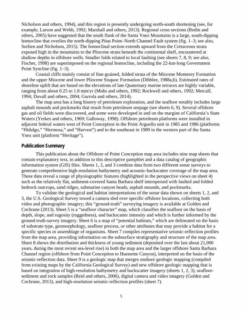
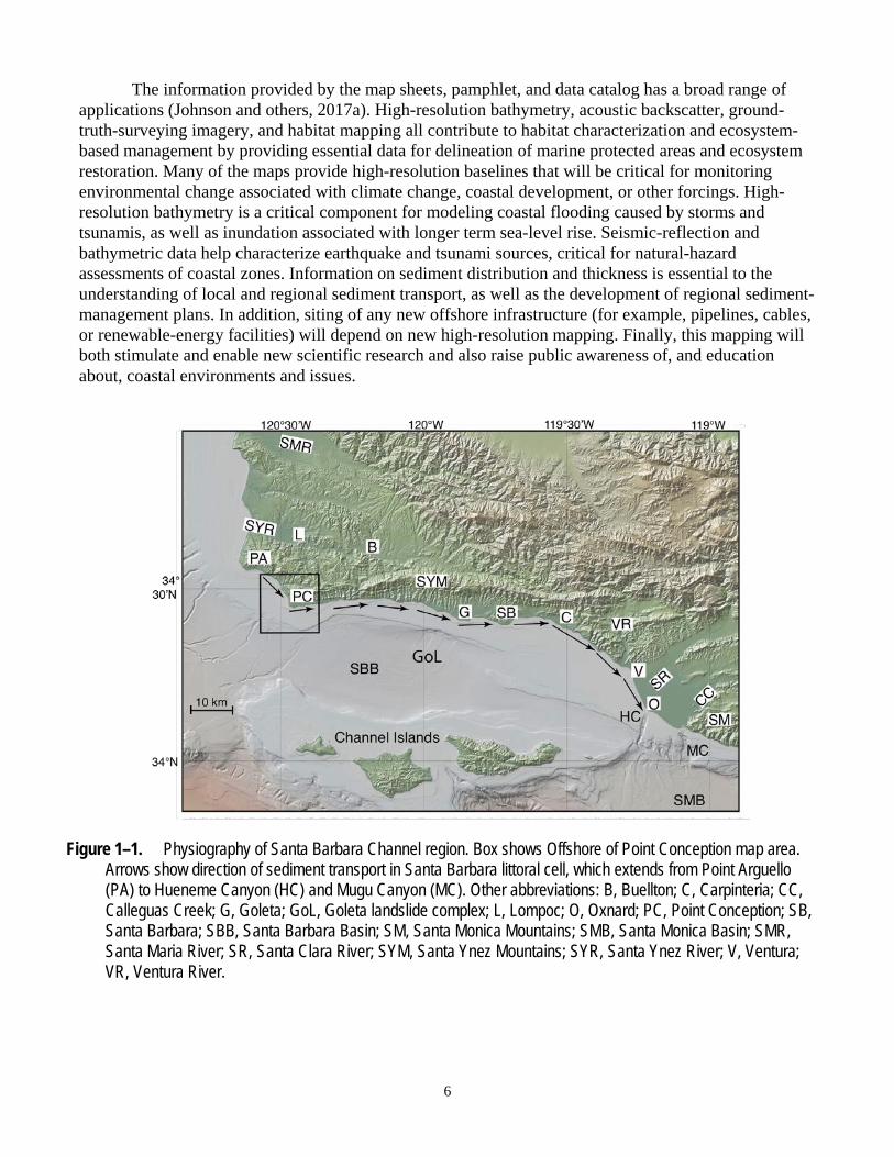
The onland part of the coastal zone is remote and sparsely populated (fig. 1–2). The road to Jalama Beach County Park provides the only public coastal access in the entire map area. North of this county park, the coastal zone is part of Vandenberg Air Force Base, which functions primarily as a space and missile testing facility. South of Jalama Beach County Park, most of the coastal zone is part of the Cojo-Jalama Ranch, purchased by the Nature Conservancy in December 2017. A relatively small part of the coastal zone in the eastern part of the map area lies within the privately owned Hollister Ranch. The nearest significant commercial centers are Lompoc (population, about 42,000), about 10 km north of the map area, and Goleta (population, about 30,000), about 50 km east of the map area. The Union Pacific railroad tracks run west and northwest along the coast through the entire map area, within a few hundred meters of the shoreline.

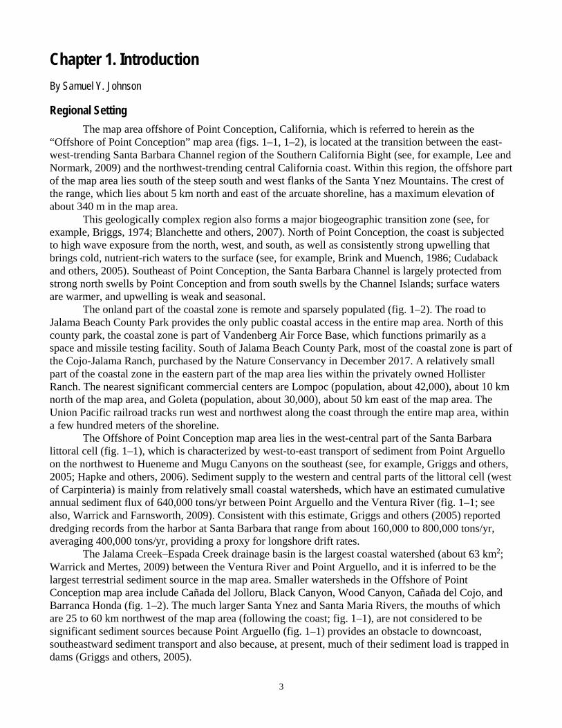
The Offshore of Point Conception map area lies in the west-central part of the Santa Barbara littoral cell (fig. 1–1), which is characterized by west-to-east transport of sediment from Point Arguello on the northwest to Hueneme and Mugu Canyons on the southeast (see, for example, Griggs and others, 2005; Hapke and others, 2006). Sediment supply to the western and central parts of the littoral cell (west of Carpinteria) is mainly from relatively small coastal watersheds, which have an estimated cumulative annual sediment flux of 640,000 tons/yr between Point Arguello and the Ventura River (fig. 1–1; see also, Warrick and Farnsworth, 2009). Consistent with this estimate, Griggs and others (2005) reported dredging records from the harbor at Santa Barbara that range from about 160,000 to 800,000 tons/yr, averaging 400,000 tons/yr, providing a proxy for longshore drift rates.

The Jalama Creek–Espada Creek drainage basin is the largest coastal watershed (about 63 km2; Warrick and Mertes, 2009) between the Ventura River and Point Arguello, and it is inferred to be the largest terrestrial sediment source in the map area. Smaller watersheds in the Offshore of Point Conception map area include Cañada del Jolloru, Black Canyon, Wood Canyon, Cañada del Cojo, and Barranca Honda (fig. 1–2). The much larger Santa Ynez and Santa Maria Rivers, the mouths of which are 25 to 60 km northwest of the map area (following the coast; fig. 1–1), are not considered to be significant sediment sources because Point Arguello (fig. 1–1) provides an obstacle to downcoast, southeastward sediment transport and also because, at present, much of their sediment load is trapped in dams (Griggs and others, 2005).

4

Coastal-watershed discharge and sediment load are highly variable, characterized by brief large events during major winter storms and long periods of low (or no) flow and minimal sediment load between storms. In recent (recorded) history, the majority of high-discharge, high-sediment-flux events have been associated with El Niño phases of the El Niño–Southern Oscillation (ENSO) climatic pattern (Warrick and Farnsworth, 2009).

Narrow beaches that have thin sediment (sand and pebbles) cover above bedrock platforms, backed by low (10- to 20-m-high) cliffs that are capped by a narrow coastal terrace, characterize much of the shoreline in the Offshore of Point Conception map area. Beaches are subject to wave erosion during winter storms, followed by gradual sediment recovery or accretion in the late spring, summer, and fall months during the gentler wave climate. Hapke and others (2006, their fig. 33) suggested that essentially no net change (accretion or erosion) to the beaches in the map area has occurred in the long term (since the mid- to late-1800s); however, the beaches have been eroding at an average rate of about 1 m/yr in the short term (1976 to 1998). Hapke and Reid (2007, their fig. 29) also indicated that coastal bluffs in the map area are eroding at a rate of about 0.2 to 0.3 m/yr. As with stream discharge and sediment flux, coastal erosion has been most acute during El Niño phases of the ENSO climatic pattern.

Following the coastline, the shelf bends to the north and northwest around Point Conception, and the trend of the shelf break (which is mostly outside California’s State Waters) changes from about 298° to 241° azimuth. Shelf width ranges from about 5 km south of Point Conception to about 11 km northwest of it; the slope ranges from about 1.0° to 1.2° to about 0.7° south and northwest of Point Conception, respectively. Southwest of Point Conception, the shelf break and upper slope are incised by a 600-m-wide, 20- to 30-m-deep, south-facing trough, one of five heads of the informally named Arguello submarine canyon (fig. 1–2; Greene and others, 1991; Eichhubl and others, 2002; Monterey Bay Aquarium Research Institute, 2002).

Significant parts of the shelf are underlain by bedrock or by bedrock that has a very thin (<1m) sediment cover (see sheets 7, 8); mean and maximum sediment thicknesses are 2.7 and 18 m, respectively. The thickest sediment is found west of Point Conception along the axis of Government Point Syncline (see sheets 7, 8, 9) and also offshore of the mouth of Jalama Creek.

Seafloor habitats in the broad Santa Barbara Channel region consist of significant amounts of soft, unconsolidated sediment interspersed with isolated areas of rocky habitat that support kelp-forest communities in the nearshore and rocky-reef communities in deeper water. The potential marine benthic habitat types mapped in the Offshore of Point Conception map area are directly related to its Quaternary geologic history, geomorphology, and active sedimentary processes. These potential habitats lie primarily within the Shelf (continental shelf) but also partly within the Flank (basin flank or continental slope) megahabitats of Greene and others (2007). The fairly homogeneous seafloor of sediment and low- relief bedrock provides characteristic habitat for groundfish, crabs, shrimp, and other marine benthic organisms, and the bedrock outcrops are potential benthic habitats for rockfish (Sebastes spp.) and other groundfish that forage and seek refuge in such habitats. In addition, several areas of smooth sediment that form nearshore terraces that have relatively steep, smooth fronts may provide interfaces attractive to certain species of groundfish. Below the steep shelf break, within the basin flank or continental slope megahabitat, the seafloor is composed of soft, unconsolidated sediment interrupted by the heads of several submarine canyons, gullies, and rills; this steep relief also provides good potential habitat for rockfish. The map area includes the large (58.3 km2) Point Conception State Marine Reserve (fig. 1–2).

The Offshore of Point Conception map area is in the westernmost part of the Western Transverse Ranges geologic province, which is north of the California Continental Borderland5 (Fisher and others, 2009). Significant clockwise rotation—at least 90°—since the early Miocene has been proposed for the Western Transverse Ranges province (Luyendyk and others, 1980; Hornafius and others, 1986;

5 The California Continental Borderland is defined as the complex continental margin that extends from Point Conception south into northern Baja California.

5

Nicholson and others, 1994), and this region is presently undergoing north-south shortening (see, for example, Larson and Webb, 1992; Marshall and others, 2013). Regional cross sections (Redin and others, 2005) have suggested that the south flank of the Santa Ynez Mountains is a large, south-dipping homocline that overlies the north-dipping Pitas Point–North Channel Fault system (fig. 1–3; see also, Sorlien and Nicholson, 2015). The homoclinal section extends upward from the Cretaceous strata exposed high in the mountains to the Pliocene strata beneath the continental shelf, encountered at shallow depths in offshore wells. Smaller folds related to local faulting (see sheets 7, 8, 9; see also, Fischer, 1998) are superimposed on the regional homocline, including the 22-km-long Government Point Syncline (fig. 1–3).

Coastal cliffs mainly consist of fine-grained, folded strata of the Miocene Monterey Formation and the upper Miocene and lower Pliocene Sisquoc Formation (Dibblee, 1988a,b). Estimated rates of shoreline uplift that are based on the elevations of late Quaternary marine terraces are highly variable, ranging from about 0.25 to 1.8 mm/yr (Muhs and others, 1992; Rockwell and others, 1992; Metcalf, 1994; Duvall and others, 2004; Gurrola and others, 2014).

The map area has a long history of petroleum exploration, and the seafloor notably includes large asphalt mounds and pockmarks that result from petroleum seepage (see sheets 6, 9). Several offshore gas and oil fields were discovered, and some were developed in and on the margins of California’s State Waters (Yerkes and others, 1969; Galloway, 1998). Offshore petroleum platforms were installed in adjacent federal waters west of Point Conception in the Point Arguello unit in 1985 and 1986 (platforms “Hidalgo,” “Hermosa,” and “Harvest”) and to the southeast in 1989 in the western part of the Santa Ynez unit (platform “Heritage”).

Publication Summary

This publication about the Offshore of Point Conception map area includes nine map sheets that contain explanatory text, in addition to this descriptive pamphlet and a data catalog of geographic information system (GIS) files. Sheets 1, 2, and 3 combine data from two different sonar surveys to generate comprehensive high-resolution bathymetry and acoustic-backscatter coverage of the map area. These data reveal a range of physiographic features (highlighted in the perspective views on sheet 4) such as the relatively flat, sediment-covered Santa Barbara shelf interspersed with faulted and folded bedrock outcrops, sand ridges, submarine canyon heads, asphalt mounds, and pockmarks.

To validate the geological and habitat interpretations of the sonar data shown on sheets 1, 2, and 3, the U.S. Geological Survey towed a camera sled over specific offshore locations, collecting both video and photographic imagery; this “ground-truth” surveying imagery is available at Golden and Cochrane (2013). Sheet 5 is a “seafloor character” map, which classifies the seafloor on the basis of depth, slope, and rugosity (ruggedness), and backscatter intensity and which is further informed by the ground-truth-survey imagery. Sheet 6 is a map of “potential habitats,” which are delineated on the basis of substrate type, geomorphology, seafloor process, or other attributes that may provide a habitat for a specific species or assemblage of organisms. Sheet 7 compiles representative seismic-reflection profiles from the map area, providing information on the subsurface stratigraphy and structure of the map area. Sheet 8 shows the distribution and thickness of young sediment (deposited over the last about 21,000 years, during the most recent sea-level rise) in both the map area and the larger offshore Santa Barbara Channel region (offshore from Point Conception to Hueneme Canyon), interpreted on the basis of the seismic-reflection data. Sheet 9 is a geologic map that merges onshore geologic mapping (compiled from existing maps by the California Geological Survey) and new offshore geologic mapping that is based on integration of high-resolution bathymetry and backscatter imagery (sheets 1, 2, 3), seafloor- sediment and rock samples (Reid and others, 2006), digital camera and video imagery (Golden and Cochrane, 2013), and high-resolution seismic-reflection profiles (sheet 7).

6

The information provided by the map sheets, pamphlet, and data catalog has a broad range of applications (Johnson and others, 2017a). High-resolution bathymetry, acoustic backscatter, ground- truth-surveying imagery, and habitat mapping all contribute to habitat characterization and ecosystem- based management by providing essential data for delineation of marine protected areas and ecosystem restoration. Many of the maps provide high-resolution baselines that will be critical for monitoring environmental change associated with climate change, coastal development, or other forcings. High- resolution bathymetry is a critical component for modeling coastal flooding caused by storms and tsunamis, as well as inundation associated with longer term sea-level rise. Seismic-reflection and bathymetric data help characterize earthquake and tsunami sources, critical for natural-hazard assessments of coastal zones. Information on sediment distribution and thickness is essential to the understanding of local and regional sediment transport, as well as the development of regional sediment- management plans. In addition, siting of any new offshore infrastructure (for example, pipelines, cables, or renewable-energy facilities) will depend on new high-resolution mapping. Finally, this mapping will both stimulate and enable new scientific research and also raise public awareness of, and education about, coastal environments and issues.

Figure 1–1. Physiography of Santa Barbara Channel region. Box shows Offshore of Point Conception map area. Arrows show direction of sediment transport in Santa Barbara littoral cell, which extends from Point Arguello (PA) to Hueneme Canyon (HC) and Mugu Canyon (MC). Other abbreviations: B, Buellton; C, Carpinteria; CC, Calleguas Creek; G, Goleta; GoL, Goleta landslide complex; L, Lompoc; O, Oxnard; PC, Point Conception; SB, Santa Barbara; SBB, Santa Barbara Basin; SM, Santa Monica Mountains; SMB, Santa Monica Basin; SMR, Santa Maria River; SR, Santa Clara River; SYM, Santa Ynez Mountains; SYR, Santa Ynez River; V, Ventura; VR, Ventura River.

7

Figure 1–2. Coastal geography of Offshore of Point Conception map area. Yellow line shows 3-nautical-mile limit of California’s State Waters. Blue line shows boundary of Point Conception State Marine Reserve (PCSMR). Other abbreviations: ASC, one head of Arguello submarine canyon; BC, Black Canyon; BH, Barranca Honda; CC, Cañada del Cojo; CJ, Cañada del Jolloru; C-JR, Cojo-Jalama Ranch; EC, Espada Creek; GP, Government Point; HR, Hollister Ranch; JC, Jalama Creek; JCP, Jalama Beach County Park; PC, Point Conception; VAFB, Vandenberg Air Force Base; WC, Wood Canyon.

8

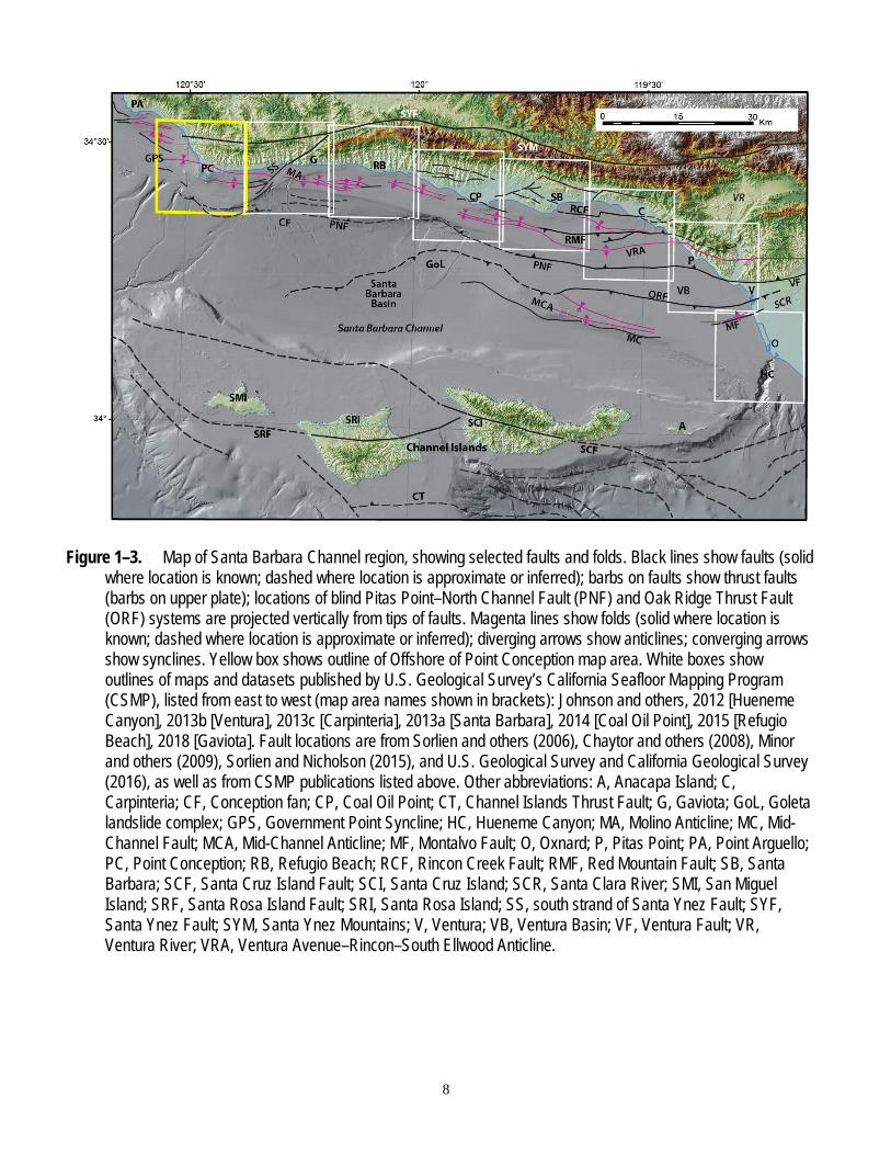
Figure 1–3. Map of Santa Barbara Channel region, showing selected faults and folds. Black lines show faults (solid where location is known; dashed where location is approximate or inferred); barbs on faults show thrust faults (barbs on upper plate); locations of blind Pitas Point–North Channel Fault (PNF) and Oak Ridge Thrust Fault (ORF) systems are projected vertically from tips of faults. Magenta lines show folds (solid where location is known; dashed where location is approximate or inferred); diverging arrows show anticlines; converging arrows show synclines. Yellow box shows outline of Offshore of Point Conception map area. White boxes show outlines of maps and datasets published by U.S. Geological Survey’s California Seafloor Mapping Program (CSMP), listed from east to west (map area names shown in brackets): Johnson and others, 2012 [Hueneme Canyon], 2013b [Ventura], 2013c [Carpinteria], 2013a [Santa Barbara], 2014 [Coal Oil Point], 2015 [Refugio Beach], 2018 [Gaviota]. Fault locations are from Sorlien and others (2006), Chaytor and others (2008), Minor and others (2009), Sorlien and Nicholson (2015), and U.S. Geological Survey and California Geological Survey (2016), as well as from CSMP publications listed above. Other abbreviations: A, Anacapa Island; C, Carpinteria; CF, Conception fan; CP, Coal Oil Point; CT, Channel Islands Thrust Fault; G, Gaviota; GoL, Goleta landslide complex; GPS, Government Point Syncline; HC, Hueneme Canyon; MA, Molino Anticline; MC, Mid- Channel Fault; MCA, Mid-Channel Anticline; MF, Montalvo Fault; O, Oxnard; P, Pitas Point; PA, Point Arguello; PC, Point Conception; RB, Refugio Beach; RCF, Rincon Creek Fault; RMF, Red Mountain Fault; SB, Santa Barbara; SCF, Santa Cruz Island Fault; SCI, Santa Cruz Island; SCR, Santa Clara River; SMI, San Miguel Island; SRF, Santa Rosa Island Fault; SRI, Santa Rosa Island; SS, south strand of Santa Ynez Fault; SYF, Santa Ynez Fault; SYM, Santa Ynez Mountains; V, Ventura; VB, Ventura Basin; VF, Ventura Fault; VR, Ventura River; VRA, Ventura Avenue–Rincon–South Ellwood Anticline.

9

Chapter 2. Bathymetry and Backscatter-Intensity Maps of the Offshore

of Point Conception Map Area (Sheets 1, 2, and 3)

By Peter Dartnell and Rikk G. Kvitek

The colored shaded-relief bathymetry (sheet 1), the shaded-relief bathymetry (sheet 2), and the acoustic-backscatter (sheet 3) maps of the Offshore of Point Conception map area in southern California were generated from bathymetry and backscatter data collected by Fugro Pelagos (fig. 1 on sheets 1, 2, 3) in 2008, using a combination of 400-kHz Reson 7125, 240-kHz Reson 8101, and 100-kHz Reson 8111 multibeam echosounders. In addition, bathymetric- and topographic-lidar data was collected in the nearshore and coastal areas by the U.S. Army Corps of Engineers (USACE) Joint Lidar Bathymetry Technical Center of Expertise in 2009 and 2010. These mapping missions combined to provide continuous bathymetry (sheets 1, 2) from the shoreline to the 3-nautical-mile limit of California’s State Waters, as well as acoustic-backscatter data (sheet 3) from about the 10-m isobath to beyond the 3- nautical-mile limit.

During the Fugro Pelagos mapping missions, an Applanix POS-MV (Position and Orientation System for Marine Vessels) was used to accurately position the vessels during data collection, and it also accounted for vessel motion such as heave, pitch, and roll, with navigational input from GPS receivers. Smoothed Best Estimated Trajectory (SBET) files were postprocessed from logged POS-MV files. Sound-velocity profiles were collected with an Applied Microsystems (AM) SVPlus sound velocimeter. Soundings were corrected for vessel motion using the Applanix POS-MV data, for variations in water-column sound velocity using the AM SVPlus data, and for variations in water height (tides) and heave using the postprocessed SBET data (California State University, Monterey Bay, Seafloor Mapping Lab, 2016). The Reson backscatter data were postprocessed using Geocoder software. The backscatter intensities were radiometrically corrected (including despeckling and angle-varying gain adjustments), and the position of each acoustic sample was geometrically corrected for slant range on a line-by-line basis. After the lines were corrected, they were mosaicked into 0.5-m resolution images (California State University, Monterey Bay, Seafloor Mapping Lab, 2016). The mosaics were then exported as georeferenced TIFF images, imported into a geographic information system (GIS), and converted to GRIDs at 2-m resolution.

Nearshore bathymetric-lidar data and acoustic-bathymetric data from within California’s State Waters were merged together as part of the 2013 National Oceanic and Atmospheric Administration (NOAA) Coastal California TopoBathy Merge Project (National Oceanic and Atmospheric Administration, 2013). Merged bathymetry data from within the Offshore of Point Conception map area were downloaded from this dataset and resampled to 2-m spatial resolution. An illumination having an azimuth of 300° and from 45° above the horizon was then applied to the bathymetric surface to create the shaded-relief imagery (sheets 1, 2). In addition, a modified “rainbow” color ramp was applied to the bathymetry data for sheet 1, using reds to represent shallower depths, and greens to represent greater depths (note that the Offshore of Point Conception map area requires only the shallower part of the full- rainbow color ramp used on some of the other maps in the California State Waters Map Series; see, for example, Kvitek and others, 2012). This colored bathymetry surface was draped over the shaded-relief imagery at 60-percent transparency to create a colored shaded-relief map (sheet 1). Note that the ripple patterns and parallel lines that are apparent within the map area are data-collection and -processing artifacts. These various artifacts are made obvious by the hillshading process.

Bathymetric contours (sheets 1, 2, 3, 5, 6, 9) were generated at 10-m intervals from a modified 2- m-resolution bathymetric surface. The most continuous contour segments were preserved; smaller segments and isolated island polygons were excluded from the final output. The contours were

10

smoothed using a polynomial approximation with exponential kernel algorithm and a tolerance value of 60 m. The contours were then clipped to the boundary of the map area.

The acoustic-backscatter imagery from each different mapping system and processing method were merged into their own individual grids. These individual grids, which cover different areas, were displayed in a GIS to create a composite acoustic-backscatter map (sheet 3). On the map, brighter tones indicate higher backscatter intensity, and darker tones indicate lower backscatter intensity. The intensity represents a complex interaction between the acoustic pulse and the seafloor, as well as characteristics within the shallow subsurface, providing a general indication of seafloor texture and composition. Backscatter intensity depends on the acoustic source level; the frequency used to image the seafloor; the grazing angle; the composition and character of the seafloor, including grain size, water content, bulk density, and seafloor roughness; and some biological cover. Harder and rougher bottom types such as rocky outcrops or coarse sediment typically return stronger intensities (high backscatter, lighter tones), whereas softer bottom types such as fine sediment return weaker intensities (low backscatter, darker tones). Ripple patterns and straight lines in some parts of the map area are data-collection and -processing artifacts.

The onshore-area image was generated by applying an illumination having an azimuth of 300° and from 45° above the horizon to 2-m-resolution topographic-lidar data from National Oceanic and Atmospheric Administration Office for Coastal Management’s Digital Coast (available at http://www.csc.noaa.gov/digitalcoast/data/coastallidar/) and to 10-m-resolution topographic-lidar data from the U.S. Geological Survey’s National Elevation Dataset (available at http://ned.usgs.gov/).

11

Chapter 3. Data Integration and Visualization for the Offshore of Point

Conception Map Area (Sheet 4)

By Peter Dartnell

Mapping California’s State Waters has produced a vast amount of acoustic and visual data, including bathymetry, acoustic backscatter, seismic-reflection profiles, and seafloor video and photography. These data are used by researchers to develop maps, reports, and other tools to assist in the coastal and marine spatial-planning capability of coastal-zone managers and other stakeholders. For example, seafloor-character (sheet 5), habitat (sheet 6), and geologic (sheet 9) maps of the Offshore of Point Conception map area may be used to assist in the designation of Marine Protected Areas, as well as in their monitoring. These maps and reports also help to analyze environmental change owing to sea- level rise and coastal development, to model and predict sediment and contaminant budgets and transport, to site offshore infrastructure, and to assess tsunami and earthquake hazards. To facilitate this increased understanding and to assist in product development, it is helpful to integrate the different datasets and then view the results in three-dimensional representations such as those displayed on the data integration and visualization sheet for the Offshore of Point Conception map area (sheet 4).

The maps and three-dimensional views on sheet 4 were created using a series of geographic information systems (GIS) and visualization techniques. Using GIS, the bathymetric and topographic data (sheet 1) were converted to ASCIIRASTER format files, and the acoustic-backscatter data (sheet 3) were converted to geoTIFF images. The bathymetric and topographic data were imported in the Fledermaus software (QPS). The bathymetry was color-coded to closely match the colored shaded- relief bathymetry on sheet 1 in which reds and oranges represent shallower depths and greens represent deeper depths. Onshore topographic data were shown in gray shades. Acoustic-backscatter geoTIFF images also were draped over the bathymetry data (fig. 6). The colored bathymetry, topography, and draped backscatter were then tilted and panned to create the perspective views such as those shown in figures 1, 2, 4, 5, and 6 on sheet 4. These views highlight the seafloor morphology in the Offshore of Point Conception map area, which includes asphalt mounds, differentially eroded bedrock, and pockmarks along the outer shelf.

Video-mosaic images created from digital seafloor video (for example, fig. 3 on sheet 4) can display the geologic (rock, sand, mud, and asphalt; see sheet 9) and biologic complexity (see Golden and Cochrane, 2013) of the seafloor. Whereas photographs capture high-quality snapshots of smaller areas of the seafloor, video mosaics capture larger areas and can show transition zones between seafloor environments. Digital seafloor video is collected from a camera sled towed approximately 1 to 2 meters above the seafloor, at speeds of less than 1 nautical mile/hour. Using standard video-editing software, as well as software developed at the Center for Coastal and Ocean Mapping, University of New Hampshire, the digital video is converted to AVI format, cut into 2-minute sections, and desampled to every second or third frame. The frames are merged together using pattern-recognition algorithms from one frame to the next and converted to a TIFF image. The images are then rectified to the bathymetry data using ship navigation recorded with the video and layback estimates of the towed camera sled.

Block diagrams that combine the bathymetry with seismic-reflection-profile data help integrate surface and subsurface observations, especially stratigraphic and structural relations (for example, fig. 2 on sheet 4). These block diagrams were created by converting digital seismic-profile data (Johnson and others, 2016) into TIFF images, while taking note of the starting and ending coordinates and maximum and minimum depths. The images were then imported into the Fledermaus software as vertical images and merged with the bathymetry imagery.

12

Chapter 4. Seafloor-Character Map of the Offshore of Point Conception

Map Area (Sheet 5)

By Guy R. Cochrane and Stephen R. Hartwell

The California State Marine Life Protection Act (MLPA) calls for protecting representative types of habitat in different depth zones and environmental conditions. A science team, assembled under the auspices of the California Department of Fish and Wildlife (CDFW), has identified seven substrate- defined seafloor habitats in California’s State Waters that can be classified using sonar data and seafloor video and photography. These habitats include rocky banks, intertidal zones, sandy or soft ocean bottoms, underwater pinnacles, kelp forests, submarine canyons, and seagrass beds. The following five depth zones, which determine changes in species composition, have been identified: Depth Zone 1, intertidal; Depth Zone 2, intertidal to 30 m; Depth Zone 3, 30 to 100 m; Depth Zone 4, 100 to 200 m; and Depth Zone 5, deeper than 200 m (California Department of Fish and Wildlife, 2008). The CDFW habitats, with the exception of depth zones, can be considered a subset of a broader classification scheme of Greene and others (1999) that has been used by the U.S. Geological Survey (USGS) (Cochrane and others, 2003, 2005). These seafloor-character maps are generalized polygon shapefiles that have attributes derived from Greene and others (2007).

A 2007 Coastal Map Development Workshop, hosted by the USGS in Menlo Park, California, identified the need for more detailed (relative to Greene and others’ [1999] attributes) raster products that preserve some of the transitional character of the seafloor when substrates are mixed and (or) they change gradationally. The seafloor-character map, which delineates a subset of the CDFW habitats, is a GIS-derived raster product that can be produced in a consistent manner from data of variable quality covering large geographic regions.

The following five substrate classes are identified in the Offshore of Point Conception map area:

• Class I: Fine- to medium-grained smooth sediment

• Class II: Mixed smooth sediment and rock

• Class III: Rock and boulder, rugose

• Class IV: Medium- to coarse-grained sediment (in scour depressions)

• Class V: Anthropogenic material (rugged)

The seafloor-character map of the Offshore of Point Conception map area (sheet 5) was produced using video-supervised maximum-likelihood classification of the bathymetry and intensity of return from sonar systems, following the method described by Cochrane (2008). The two variants used in this classification were backscatter intensity and derivative rugosity. The rugosity calculation was performed using the Terrain Ruggedness (VRM) tool within the Benthic Terrain Modeler toolset v. 3.0 (Wright and others, 2012; available at http://esriurl.com/5754).

Classes I, II, and III values were delineated using multivariate analysis. Class IV (medium- to coarse-grained sediment, in scour depressions) values were determined on the basis of their visual characteristics, using both shaded-relief bathymetry and backscatter (slight depression in the seafloor, very high backscatter return). Class V (rugged anthropogenic material) values were determined on the basis of their visual characteristics and the known location of man-made features. The resulting map (gridded at 2 m) was cleaned by hand to remove data-collection artifacts (for example, the trackline nadir).

On the seafloor-character map (sheet 5), the five substrate classes have been colored to indicate the California MLPA depth zones and the Coastal and Marine Ecological Classification Standard (CMECS) slope zones (Madden and others, 2008) in which they belong. The California MLPA depth

13

zones are Depth Zone 1 (intertidal), Depth Zone 2 (intertidal to 30 m), Depth Zone 3 (30 to 100 m), Depth Zone 4 (100 to 200 m), and Depth Zone 5 (greater than 200 m); in the Offshore of Point Conception map area, only Depth Zones 2, 3, and 4 are present. The slope classes that represent the CMECS slope zones are Slope Class 1 = flat (0° to 5°), Slope Class 2 = sloping (5° to 30°), Slope Class 3 = steeply sloping (30° to 60°), Slope Class 4 = vertical (60° to 90°), and Slope Class 5 = overhang (greater than 90°); in the Offshore of Point Conception map area, only Slope Classes 1 and 2 are present. The final classified seafloor-character raster map image has been draped over the shaded-relief bathymetry for the area (sheets 1 and 2) to produce the image shown on the seafloor-character map on sheet 5.

The seafloor-character classification also is summarized on sheet 5 in table 1. Fine- to medium- grained smooth sediment (sand and mud) makes up 83.0 percent (107.1 km2) of the map area: 13.2 percent (17.0 km2) is in Depth Zone 2, 64.5 percent (83.3 km2) is in Depth Zone 3, and 5.3 percent (6.8 km2) is in Depth Zone 4. Mixed smooth sediment (sand and gravel) and rock (that is, sediment typically forming a veneer over bedrock, or rock outcrops having little to no relief) make up 7.9 percent (10.1 km2) of the map area: 3.1 percent (4.1 km2) is in Depth Zone 2, 4.7 percent (6.1 km2) is in Depth Zone 3, and 0.1 percent (0.1 km2) is in Depth Zone 4. Rock and boulder, rugose (rocky outcrops, boulder fields, and asphalt mounds having high surficial complexity) makes up 8.8 percent (11.4 km2) of the map area: 4.7 percent (6.1 km2) is in Depth Zone 2, 2.2 percent (2.9 km2) is in Depth Zone 3, and 1.9 percent (2.4 km2) is in Depth Zone 4. Medium- to coarse-grained sediment (in scour depressions consisting of material that is coarser than the surrounding seafloor) makes up 0.2 percent (0.3 km2) of the map area: less than 0.1 percent (0.1 km2) is in Depth Zone 2, 0.2 percent (0.2 km2) is in Depth Zone 3, and less than 0.1 percent (<0.1 km2) is in Depth Zone 4. Rugged anthropogenic material makes up 0.1 percent (0.1 km2) of the map area: less than 0.1 percent (<0.1 km2) is in Depth Zone 2, and 0.1 percent (0.1 km2) is in Depth Zone 3.

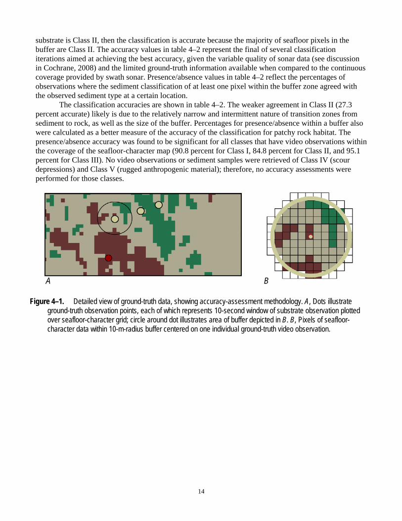
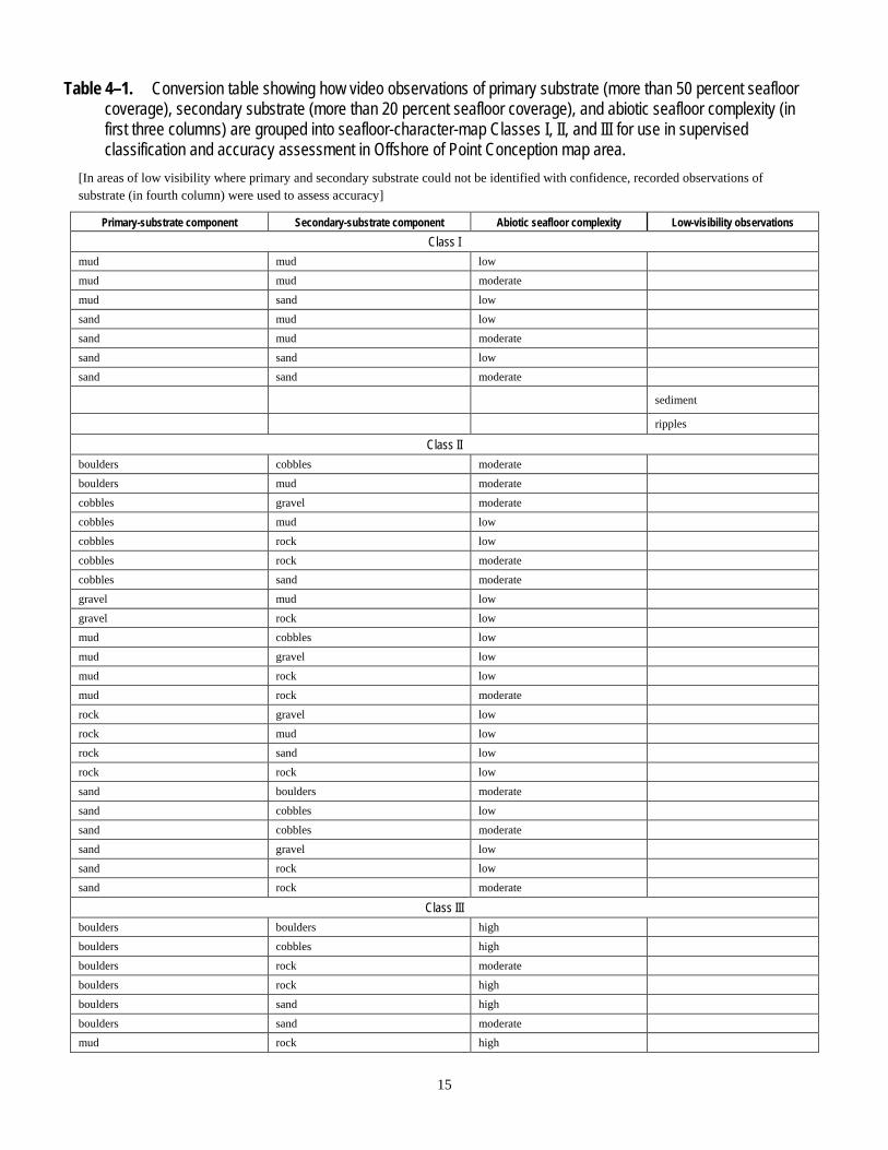
A small number of video observations and sediment samples were used to supervise the numerical classification of the seafloor. All video observations (see Golden and Cochrane, 2013) are used for accuracy assessment of the seafloor-character map after classification. To compare observations to classified pixels, each observation point is assigned a class (I, II, or III) according to the visually derived, major or minor geologic component (for example, sand or rock) and the abiotic complexity (vertical variability) of the substrate recorded during ground-truth surveys (table 4–1; see also, Golden and Cochrane, 2013). Class IV values were assigned on the basis of the observation of one or more of a group of features that includes both larger scale bedforms (for example, sand waves), as well as sediment-filled scour depressions that resemble the “rippled scour depressions” of Cacchione and others (1984), Hallenbeck and others (2012); and Davis and others (2013) and also the “sorted bedforms” of Murray and Thieler (2004), Goff and others (2005), and Trembanis and Hume (2011). On the geologic map (see sheet 9 of this report), they are referred to as “marine shelf scour depressions.” Class V values are determined from the visual characteristics and known locations of man-made features.

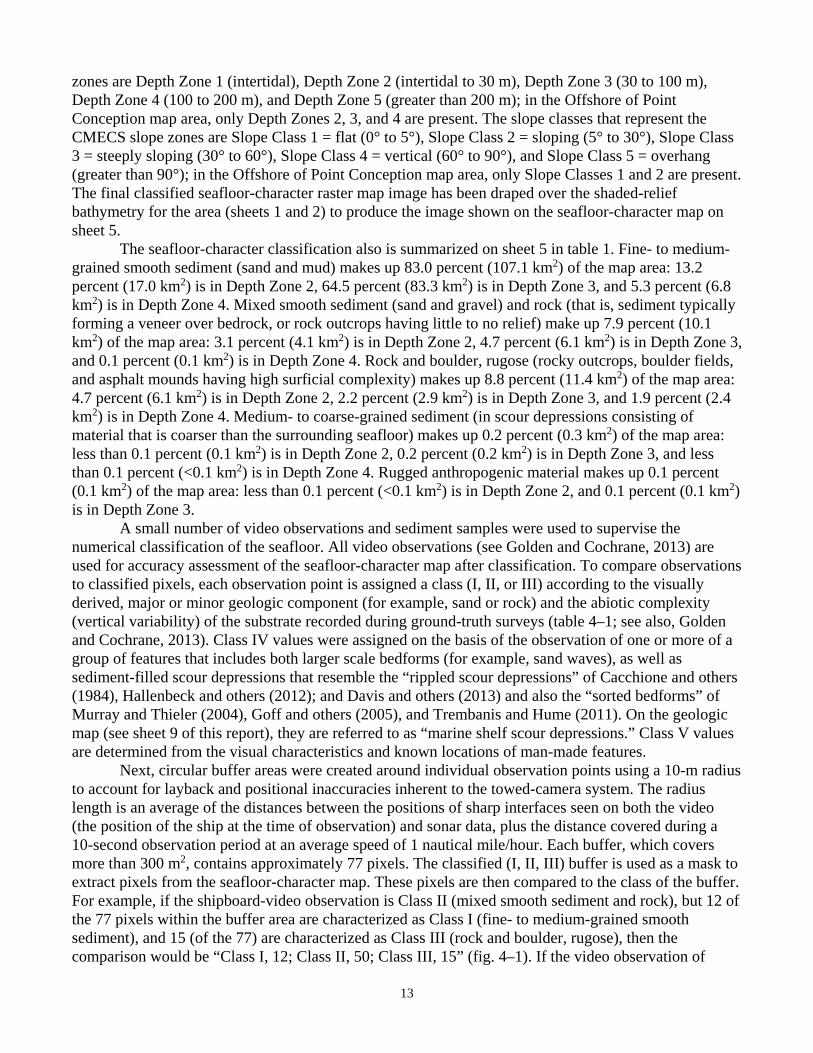
Next, circular buffer areas were created around individual observation points using a 10-m radius to account for layback and positional inaccuracies inherent to the towed-camera system. The radius length is an average of the distances between the positions of sharp interfaces seen on both the video (the position of the ship at the time of observation) and sonar data, plus the distance covered during a 10-second observation period at an average speed of 1 nautical mile/hour. Each buffer, which covers more than 300 m2, contains approximately 77 pixels. The classified (I, II, III) buffer is used as a mask to extract pixels from the seafloor-character map. These pixels are then compared to the class of the buffer. For example, if the shipboard-video observation is Class II (mixed smooth sediment and rock), but 12 of the 77 pixels within the buffer area are characterized as Class I (fine- to medium-grained smooth sediment), and 15 (of the 77) are characterized as Class III (rock and boulder, rugose), then the comparison would be “Class I, 12; Class II, 50; Class III, 15” (fig. 4–1). If the video observation of

14

substrate is Class II, then the classification is accurate because the majority of seafloor pixels in the buffer are Class II. The accuracy values in table 4–2 represent the final of several classification iterations aimed at achieving the best accuracy, given the variable quality of sonar data (see discussion in Cochrane, 2008) and the limited ground-truth information available when compared to the continuous coverage provided by swath sonar. Presence/absence values in table 4–2 reflect the percentages of observations where the sediment classification of at least one pixel within the buffer zone agreed with the observed sediment type at a certain location.

The classification accuracies are shown in table 4–2. The weaker agreement in Class II (27.3 percent accurate) likely is due to the relatively narrow and intermittent nature of transition zones from sediment to rock, as well as the size of the buffer. Percentages for presence/absence within a buffer also were calculated as a better measure of the accuracy of the classification for patchy rock habitat. The presence/absence accuracy was found to be significant for all classes that have video observations within the coverage of the seafloor-character map (90.8 percent for Class I, 84.8 percent for Class II, and 95.1 percent for Class III). No video observations or sediment samples were retrieved of Class IV (scour depressions) and Class V (rugged anthropogenic material); therefore, no accuracy assessments were performed for those classes.

Figure 4–1. Detailed view of ground-truth data, showing accuracy-assessment methodology. A, Dots illustrate ground-truth observation points, each of which represents 10-second window of substrate observation plotted over seafloor-character grid; circle around dot illustrates area of buffer depicted in B. B, Pixels of seafloor- character data within 10-m-radius buffer centered on one individual ground-truth video observation.

15

Table 4–1. Conversion table showing how video observations of primary substrate (more than 50 percent seafloor coverage), secondary substrate (more than 20 percent seafloor coverage), and abiotic seafloor complexity (in first three columns) are grouped into seafloor-character-map Classes I, II, and III for use in supervised classification and accuracy assessment in Offshore of Point Conception map area.

[In areas of low visibility where primary and secondary substrate could not be identified with confidence, recorded observations of substrate (in fourth column) were used to assess accuracy]

Primary-substrate component Secondary-substrate component Abiotic seafloor complexity Low-visibility observations Class I

mud mud low

mud mud moderate

mud sand low

sand mud low

sand mud moderate

sand sand low

sand sand moderate

sediment

ripples

Class II boulders cobbles moderate

boulders mud moderate

cobbles gravel moderate

cobbles mud low

cobbles rock low

cobbles rock moderate

cobbles sand moderate

gravel mud low

gravel rock low

mud cobbles low

mud gravel low

mud rock low

mud rock moderate

rock gravel low

rock mud low

rock sand low

rock rock low

sand boulders moderate

sand cobbles low

sand cobbles moderate

sand gravel low

sand rock low

sand rock moderate

Class III boulders boulders high

boulders cobbles high

boulders rock moderate

boulders rock high

boulders sand high

boulders sand moderate

mud rock high

16

Table 4–1. Conversion table showing how video observations of primary substrate (more than 50 percent seafloor coverage), secondary substrate (more than 20 percent seafloor coverage), and abiotic seafloor complexity (in first three columns) are grouped into seafloor-character-map Classes I, II, and III for use in supervised classification and accuracy assessment in Offshore of Point Conception map area.—Continued

Primary-substrate component Secondary-substrate component Abiotic seafloor complexity Low-visibility observations Class III—Continued

rock boulders high

rock boulders moderate

rock cobbles moderate

rock mud moderate

rock rock high

rock rock moderate

rock sand high

rock sand moderate

sand rock high

Table 4–2. Accuracy-assessment statistics for seafloor-character-map classifications in Offshore of Point Conception map area.

[Accuracy assessments are based on video observations (N/A, no accuracy assessment was conducted)]

Class Number of observations % majority % presence/absence

I—Fine- to medium-grained smooth sediment 196 76.0 90.8

II—Mixed smooth sediment and rock 66 27.3 84.8

III—Rock and boulder, rugose 41 73.2 95.1

IV—Medium- to coarse-grained sediment (in scour depressions) 0 N/A N/A

V—Rugged anthropogenic material 0 N/A N/A

17

Chapter 5. Marine Benthic Habitats of the Offshore of Point Conception

Map Area (Sheet 6)

By Guy R. Cochrane and Stephen R. Hartwell

The map on sheet 6 shows physical marine benthic habitats in the Offshore of Point Conception map area. Marine benthic habitats represent a particular type of substrate and geomorphology that may provide a habitat for a specific species or assemblage of organisms. Marine benthic habitats are classified using the Coastal and Marine Ecological Classification Standard (CMECS), developed by representatives from a consortium of Federal agencies. CMECS is the Federal standard for marine habitat characterization (available at https://www.fgdc.gov/standards/projects/FGDC-standards- projects/cmecs-folder/CMECS_Version_06-2012_FINAL.pdf). The standard provides an ecologically relevant structure for biologic-, geologic-, chemical-, and physical-habitat attributes.

The map illustrates the geoform and substrate components of the CMECS standard and their distribution in the Offshore of Point Conception map area. Geoform components describe the major geomorphic and structural characteristics of the coast and seafloor (that is, the tectonic and physiographic settings and the geological, biogenic, and anthropogenic features). The map was derived from the geologic and geomorphic map of the seafloor (see sheet 9) by translation of the map-unit descriptions into the best-fit values of the CMECS classes. A geoform is found in the CMECS description when the geologic map-unit description includes a geomorphologic element. Geologic map units that lack grain size information, such as anthropogenic features, will correspondingly lack a CMECS substrate classification. The map also includes a temporal attribute for each unit that indicates time period of persistence, as well as an induration attribute that allows resymbolization of the data- catalog shapefile into a simple map of hard-mixed-soft attributes essential for fish-habitat assessment.

CMECS codes are provided in the data-catalog shapefile and in table 5–1 (the CMECS coding system is described at https://coast.noaa.gov/digitalcoast/sites/default/files/files/publications/21072015/ CMECS_Coding_System_Approach_20140619.pdf). Note that the CMECS codes are designed to facilitate database searching and sorting but are not used for map symbolization on the benthic habitat map (sheet 6); instead, polygons are labeled with a letter that identifies the CMECS physiographic setting (S, continental shelf; L, continental slope) and a number for each map unit within that setting (table 5–1).

Map Area Habitats

The Offshore of Point Conception map area includes the continental shelf and small parts of the upper slope, in a major transitional zone between the exposed, northwest-trending central California coast and the more protected, east-west-trending coast of the Santa Barbara Channel. Delineated on the map are 13 marine benthic habitat types: 11 types are located on the continental shelf, and 2 are located on the slope (table 5–1; see also table 1 on sheet 6). The habitats include soft, unconsolidated sediment (9 habitat types) such as fine sand and mud and also just sand, as well as dynamic features such as mobile sand sheets, sediment waves, and rippled sediment depressions; mixed substrate (1 habitat type) such as intermittent sands that overlie hard consolidated bedrock; and hard substrate (2 habitat types) such as bedrock. In addition, one habitat that contains anthropogenic features (a wreck) is mapped in the map area.

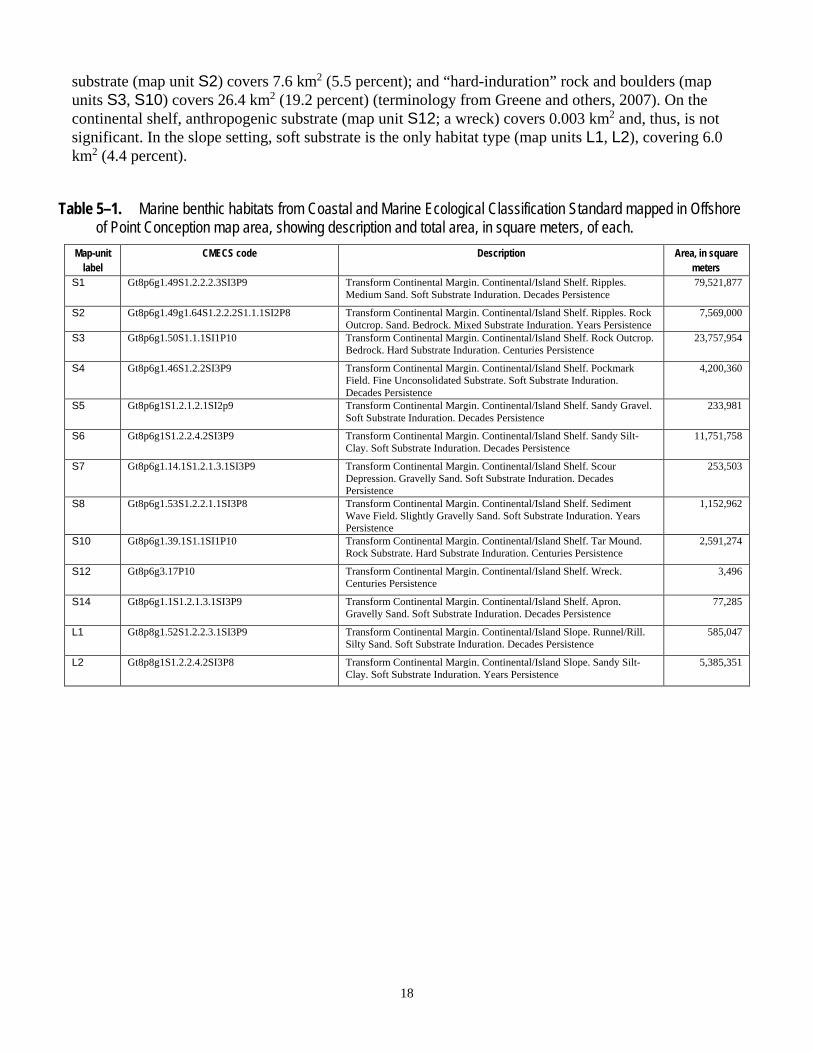
Of the total of 137.1 km2 mapped in the Offshore of Point Conception map area, 131.1 km2 (95.6 percent) is mapped in the continental shelf setting, and 6.0 km2 (4.4 percent) is mapped in the slope setting. In the continental shelf setting, “soft-induration” unconsolidated sediment is the dominant habitat type (map units S1, S4–S8, S14), covering 97.2 km2 (70.9 percent); “mixed-induration”

18

substrate (map unit S2) covers 7.6 km2 (5.5 percent); and “hard-induration” rock and boulders (map units S3, S10) covers 26.4 km2 (19.2 percent) (terminology from Greene and others, 2007). On the continental shelf, anthropogenic substrate (map unit S12; a wreck) covers 0.003 km2 and, thus, is not significant. In the slope setting, soft substrate is the only habitat type (map units L1, L2), covering 6.0 km2 (4.4 percent).

Table 5–1. Marine benthic habitats from Coastal and Marine Ecological Classification Standard mapped in Offshore of Point Conception map area, showing description and total area, in square meters, of each.

Map-unit label

CMECS code Description Area, in square meters

S1 Gt8p6g1.49S1.2.2.2.3SI3P9 Transform Continental Margin. Continental/Island Shelf. Ripples. Medium Sand. Soft Substrate Induration. Decades Persistence

79,521,877

S2 Gt8p6g1.49g1.64S1.2.2.2S1.1.1SI2P8 Transform Continental Margin. Continental/Island Shelf. Ripples. Rock Outcrop. Sand. Bedrock. Mixed Substrate Induration. Years Persistence

7,569,000

S3 Gt8p6g1.50S1.1.1SI1P10 Transform Continental Margin. Continental/Island Shelf. Rock Outcrop. Bedrock. Hard Substrate Induration. Centuries Persistence

23,757,954

S4 Gt8p6g1.46S1.2.2SI3P9 Transform Continental Margin. Continental/Island Shelf. Pockmark Field. Fine Unconsolidated Substrate. Soft Substrate Induration. Decades Persistence

4,200,360

S5 Gt8p6g1S1.2.1.2.1SI2p9 Transform Continental Margin. Continental/Island Shelf. Sandy Gravel. Soft Substrate Induration. Decades Persistence

233,981

S6 Gt8p6g1S1.2.2.4.2SI3P9 Transform Continental Margin. Continental/Island Shelf. Sandy Silt-Clay. Soft Substrate Induration. Decades Persistence

11,751,758

S7 Gt8p6g1.14.1S1.2.1.3.1SI3P9 Transform Continental Margin. Continental/Island Shelf. Scour Depression. Gravelly Sand. Soft Substrate Induration. Decades Persistence

253,503

S8 Gt8p6g1.53S1.2.2.1.1SI3P8 Transform Continental Margin. Continental/Island Shelf. Sediment Wave Field. Slightly Gravelly Sand. Soft Substrate Induration. Years Persistence

1,152,962

S10 Gt8p6g1.39.1S1.1SI1P10 Transform Continental Margin. Continental/Island Shelf. Tar Mound. Rock Substrate. Hard Substrate Induration. Centuries Persistence

2,591,274

S12 Gt8p6g3.17P10 Transform Continental Margin. Continental/Island Shelf. Wreck. Centuries Persistence

3,496

S14 Gt8p6g1.1S1.2.1.3.1SI3P9 Transform Continental Margin. Continental/Island Shelf. Apron. Gravelly Sand. Soft Substrate Induration. Decades Persistence

77,285

L1 Gt8p8g1.52S1.2.2.3.1SI3P9 Transform Continental Margin. Continental/Island Slope. Runnel/Rill. Silty Sand. Soft Substrate Induration. Decades Persistence

585,047

L2 Gt8p8g1S1.2.2.4.2SI3P8 Transform Continental Margin. Continental/Island Slope. Sandy Silt-Clay. Soft Substrate Induration. Years Persistence

5,385,351

19

Chapter 6. Subsurface Geology and Structure of the Offshore of Point

Conception Map Area and the Santa Barbara Channel Region (Sheets 7

and 8)

By Samuel Y. Johnson and Stephen R. Hartwell

The seismic-reflection profiles presented on sheet 7 provide a third dimension—depth beneath the seafloor—to complement the surficial seafloor-mapping data already presented (sheets 1 through 6) for the Offshore of Point Conception map area. These data, which are collected at several resolutions, extend to varying depths in the subsurface, depending on the purpose and mode of data acquisition. The seismic-reflection profiles (sheet 7) provide information on sediment character, distribution, and thickness; the profiles also provide information on potential geologic hazards, which include active faults, areas that are prone to strong ground motion, and areas that have potential for tsunamigenic slope failures. The information on faults provides essential input to national and state earthquake-hazard maps and assessments (see, for example, Petersen and others, 2014).

The maps on sheet 8 show the following interpretations, which are based on the seismic- reflection profiles on sheet 7: the thickness of the composite uppermost Pleistocene and Holocene sediment unit; the depth to base of this uppermost unit; and both the local and regional distribution of faults (includes new data from this report, as well as from Jennings and Bryant, 2010; U.S. Geological Survey and California Geological Survey, 2016; and Johnson and others, 2017b) and earthquake epicenters (U.S. Geological Survey, 2016).

Data Acquisition

Most profiles displayed on sheet 7 (figs. 1, 2, 3, 4, 5, 6, 7, 8, 9, 11, 12) were collected in 2014 on U.S. Geological Survey (USGS) cruise S–01–13–SC, using the SIG 2Mille minisparker system. This system used a 500-J high-voltage electrical discharge fired 1 to 2 times per second, which, at normal survey speeds of 4 to 4.5 nautical miles per hour, gives a data trace every 1 to 2 m of lateral distance covered. The data were digitally recorded in standard SEG-Y 32-bit floating-point format, using Triton Subbottom Logger (SBL) software that merges seismic-reflection data with differential GPS-navigation data. After the survey, a short-window (20 ms) automatic gain control algorithm was applied to the data, along with a 160- to 1,200-Hz bandpass filter and a heave correction that uses an automatic seafloor- detection window (averaged over 30 m of lateral distance covered). These data can resolve geologic features a few meters thick (and, hence, are considered “high-resolution”), down to subbottom depths of as much as 400 m.

Figure 10 on sheet 7 shows a migrated, multichannel seismic-reflection profile collected in 1984 by WesternGeco on cruise W–37–84–SC. This profile and other similar data were collected in many areas offshore of California in the 1970s and 1980s when these areas were considered a frontier for oil and gas exploration. Much of these data have been publicly released and are now archived at the U.S. Geological Survey National Archive of Marine Seismic Surveys (Triezenberg and others, 2016). These data were acquired using a large-volume air-gun source that has a frequency range of 3 to 40 Hz and recorded with a multichannel hydrophone streamer about 2 km long. Shot spacing was about 30 m. These data can resolve geologic features that are 20 to 30 m thick, down to subbottom depths of as much as 4 km.

Seismic-Reflection Imaging of the Continental Shelf

Sheet 7 shows seismic-reflection profiles in the offshore part of the Offshore of Point Conception map area, providing an image of the subsurface geology. The map area is characterized by a relatively

20

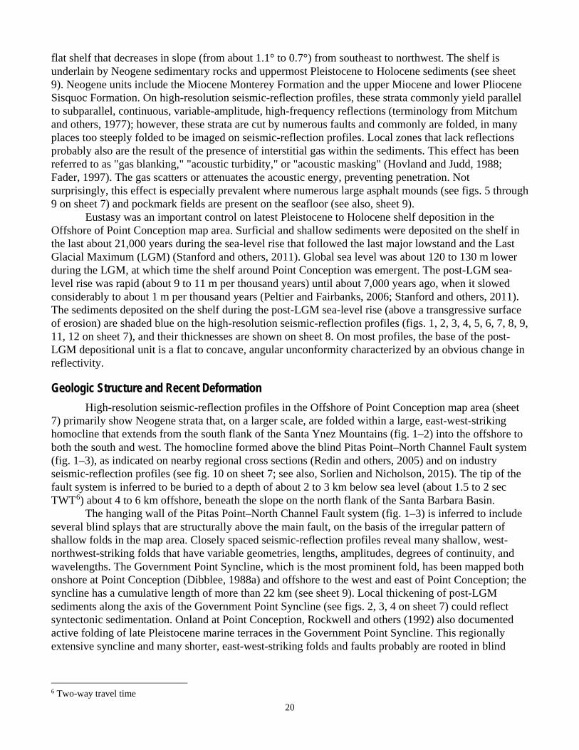
flat shelf that decreases in slope (from about 1.1° to 0.7°) from southeast to northwest. The shelf is underlain by Neogene sedimentary rocks and uppermost Pleistocene to Holocene sediments (see sheet 9). Neogene units include the Miocene Monterey Formation and the upper Miocene and lower Pliocene Sisquoc Formation. On high-resolution seismic-reflection profiles, these strata commonly yield parallel to subparallel, continuous, variable-amplitude, high-frequency reflections (terminology from Mitchum and others, 1977); however, these strata are cut by numerous faults and commonly are folded, in many places too steeply folded to be imaged on seismic-reflection profiles. Local zones that lack reflections probably also are the result of the presence of interstitial gas within the sediments. This effect has been referred to as "gas blanking," "acoustic turbidity," or "acoustic masking" (Hovland and Judd, 1988; Fader, 1997). The gas scatters or attenuates the acoustic energy, preventing penetration. Not surprisingly, this effect is especially prevalent where numerous large asphalt mounds (see figs. 5 through 9 on sheet 7) and pockmark fields are present on the seafloor (see also, sheet 9).

Eustasy was an important control on latest Pleistocene to Holocene shelf deposition in the Offshore of Point Conception map area. Surficial and shallow sediments were deposited on the shelf in the last about 21,000 years during the sea-level rise that followed the last major lowstand and the Last Glacial Maximum (LGM) (Stanford and others, 2011). Global sea level was about 120 to 130 m lower during the LGM, at which time the shelf around Point Conception was emergent. The post-LGM sea- level rise was rapid (about 9 to 11 m per thousand years) until about 7,000 years ago, when it slowed considerably to about 1 m per thousand years (Peltier and Fairbanks, 2006; Stanford and others, 2011). The sediments deposited on the shelf during the post-LGM sea-level rise (above a transgressive surface of erosion) are shaded blue on the high-resolution seismic-reflection profiles (figs. 1, 2, 3, 4, 5, 6, 7, 8, 9, 11, 12 on sheet 7), and their thicknesses are shown on sheet 8. On most profiles, the base of the post- LGM depositional unit is a flat to concave, angular unconformity characterized by an obvious change in reflectivity.

Geologic Structure and Recent Deformation

High-resolution seismic-reflection profiles in the Offshore of Point Conception map area (sheet 7) primarily show Neogene strata that, on a larger scale, are folded within a large, east-west-striking homocline that extends from the south flank of the Santa Ynez Mountains (fig. 1–2) into the offshore to both the south and west. The homocline formed above the blind Pitas Point–North Channel Fault system (fig. 1–3), as indicated on nearby regional cross sections (Redin and others, 2005) and on industry seismic-reflection profiles (see fig. 10 on sheet 7; see also, Sorlien and Nicholson, 2015). The tip of the fault system is inferred to be buried to a depth of about 2 to 3 km below sea level (about 1.5 to 2 sec TWT6) about 4 to 6 km offshore, beneath the slope on the north flank of the Santa Barbara Basin.

The hanging wall of the Pitas Point–North Channel Fault system (fig. 1–3) is inferred to include several blind splays that are structurally above the main fault, on the basis of the irregular pattern of shallow folds in the map area. Closely spaced seismic-reflection profiles reveal many shallow, west- northwest-striking folds that have variable geometries, lengths, amplitudes, degrees of continuity, and wavelengths. The Government Point Syncline, which is the most prominent fold, has been mapped both onshore at Point Conception (Dibblee, 1988a) and offshore to the west and east of Point Conception; the syncline has a cumulative length of more than 22 km (see sheet 9). Local thickening of post-LGM sediments along the axis of the Government Point Syncline (see figs. 2, 3, 4 on sheet 7) could reflect syntectonic sedimentation. Onland at Point Conception, Rockwell and others (1992) also documented active folding of late Pleistocene marine terraces in the Government Point Syncline. This regionally extensive syncline and many shorter, east-west-striking folds and faults probably are rooted in blind

6 Two-way travel time

21

thrust faults and back-thrust faults in the hanging wall above the Pitas Point–North Channel Fault system (fig. 1–3).

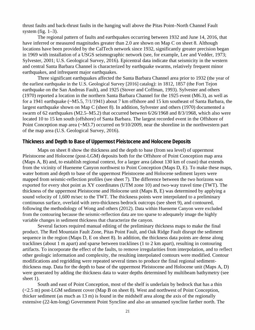
The regional pattern of faults and earthquakes occurring between 1932 and June 14, 2016, that have inferred or measured magnitudes greater than 2.0 are shown on Map C on sheet 8. Although locations have been provided by the CalTech network since 1932, significantly greater precision began in 1969 with installation of a USGS seismographic network (see, for example, Lee and Vedder, 1973; Sylvester, 2001; U.S. Geological Survey, 2016). Epicentral data indicate that seismicity in the western and central Santa Barbara Channel is characterized by earthquake swarms, relatively frequent minor earthquakes, and infrequent major earthquakes.

Three significant earthquakes affected the Santa Barbara Channel area prior to 1932 (the year of the earliest earthquake in the U.S. Geological Survey [2016] catalog): in 1812, 1857 (the Fort Tejon earthquake on the San Andreas Fault), and 1925 (Stover and Coffman, 1993). Sylvester and others (1970) reported a location in the northern Santa Barbara Channel for the 1925 event (M6.3), as well as for a 1941 earthquake (~M5.5, 7/1/1941) about 7 km offshore and 15 km southeast of Santa Barbara, the largest earthquake shown on Map C (sheet 8). In addition, Sylvester and others (1970) documented a swarm of 62 earthquakes (M2.5–M5.2) that occurred between 6/26/1968 and 8/3/1968, which also were located 10 to 15 km south (offshore) of Santa Barbara. The largest recorded event in the Offshore of Point Conception map area (~M3.7) occurred on 9/10/2009, near the shoreline in the northwestern part of the map area (U.S. Geological Survey, 2016).

Thickness and Depth to Base of Uppermost Pleistocene and Holocene Deposits

Maps on sheet 8 show the thickness and the depth to base (from sea level) of uppermost Pleistocene and Holocene (post-LGM) deposits both for the Offshore of Point Conception map area (Maps A, B) and, to establish regional context, for a larger area (about 130 km of coast) that extends from the vicinity of Hueneme Canyon northwest to Point Conception (Maps D, E). To make these maps, water bottom and depth to base of the uppermost Pleistocene and Holocene sediment layers were mapped from seismic-reflection profiles (see sheet 7). The difference between the two horizons was exported for every shot point as XY coordinates (UTM zone 10) and two-way travel time (TWT). The thickness of the uppermost Pleistocene and Holocene unit (Maps B, E) was determined by applying a sound velocity of 1,600 m/sec to the TWT. The thickness points were interpolated to a preliminary continuous surface, overlaid with zero-thickness bedrock outcrops (see sheet 9), and contoured, following the methodology of Wong and others (2012). Data within Hueneme Canyon were excluded from the contouring because the seismic-reflection data are too sparse to adequately image the highly variable changes in sediment thickness that characterize the canyon.

Several factors required manual editing of the preliminary thickness maps to make the final product. The Red Mountain Fault Zone, Pitas Point Fault, and Oak Ridge Fault disrupt the sediment sequence in the region (Maps D, E on sheet 8). In addition, the thickness data points are dense along tracklines (about 1 m apart) and sparse between tracklines (1 to 2 km apart), resulting in contouring artifacts. To incorporate the effect of the faults, to remove irregularities from interpolation, and to reflect other geologic information and complexity, the resulting interpolated contours were modified. Contour modifications and regridding were repeated several times to produce the final regional sediment- thickness map. Data for the depth to base of the uppermost Pleistocene and Holocene unit (Maps A, D) were generated by adding the thickness data to water depths determined by multibeam bathymetry (see sheet 1).

South and east of Point Conception, most of the shelf is underlain by bedrock that has a thin (<2.5 m) post-LGM sediment cover (Map B on sheet 8). West and northwest of Point Conception, thicker sediment (as much as 13 m) is found in the midshelf area along the axis of the regionally extensive (22-km-long) Government Point Syncline and also an unnamed syncline farther north. The

22

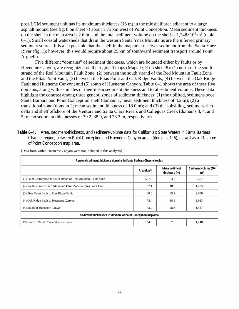
post-LGM sediment unit has its maximum thickness (18 m) in the midshelf area adjacent to a large asphalt mound (see fig. 8 on sheet 7) about 1.75 km west of Point Conception. Mean sediment thickness on the shelf in the map area is 2.6 m, and the total sediment volume on the shelf is 1,248×106 m3 (table 6–1). Small coastal watersheds that drain the western Santa Ynez Mountains are the inferred primary sediment source. It is also possible that the shelf in the map area receives sediment from the Santa Ynez River (fig. 1); however, this would require about 25 km of southward sediment transport around Point Arguello.

Five different “domains” of sediment thickness, which are bounded either by faults or by Hueneme Canyon, are recognized on the regional maps (Maps D, E on sheet 8): (1) north of the south strand of the Red Mountain Fault Zone; (2) between the south strand of the Red Mountain Fault Zone and the Pitas Point Fault; (3) between the Pitas Point and Oak Ridge Faults; (4) between the Oak Ridge Fault and Hueneme Canyon; and (5) south of Hueneme Canyon. Table 6–1 shows the area of these five domains, along with estimates of their mean sediment thickness and total sediment volume. These data highlight the contrast among three general zones of sediment thickness: (1) the uplifted, sediment-poor Santa Barbara and Point Conception shelf (domain 1; mean sediment thickness of 4.2 m); (2) a transitional zone (domain 2; mean sediment thickness of 18.0 m); and (3) the subsiding, sediment-rich delta and shelf offshore of the Ventura and Santa Clara Rivers and Calleguas Creek (domains 3, 4, and 5; mean sediment thicknesses of 39.2, 38.9, and 28.3 m, respectively).

Table 6–1. Area, sediment-thickness, and sediment-volume data for California's State Waters in Santa Barbara Channel region, between Point Conception and Hueneme Canyon areas (domains 1–5), as well as in Offshore of Point Conception map area.

[Data from within Hueneme Canyon were not included in this analysis]

Regional sediment-thickness domains in Santa Barbara Channel region

Area (km2) Mean sediment thickness (m)

Sediment volume (106

m3)

(1) Point Conception to south strand of Red Mountain Fault Zone 597.9 4.2 2,507

(2) South strand of Red Mountain Fault Zone to Pitas Point Fault 67.1 18.0 1,205

(3) Pitas Point Fault to Oak Ridge Fault 68.6 39.2 2,688

(4) Oak Ridge Fault to Hueneme Canyon 75.4 38.9 2,933

(5) South of Hueneme Canyon 53.9 28.3 1,527

Sediment thicknesses in Offshore of Point Conception map area

Offshore of Point Conception map area 154.3 2.6 1,248

23

Chapter 7. Geologic and Geomorphic Map of the Offshore of Point

Conception Map Area (Sheet 9)

By Samuel Y. Johnson and Stephen R. Hartwell

Geologic and Geomorphic Summary

Marine geology and geomorphology were mapped in the Offshore of Point Conception map area from the shoreline to the 3-nautical-mile limit of California’s State Waters. The location of the shoreline, which is from the National Oceanic and Atmospheric Administration’s (NOAA’s) Shoreline Data Explorer, is based on their analysis of lidar imagery (National Geodetic Survey, 2016). Offshore geologic units were delineated on the basis of integrated analyses of adjacent onshore geology with multibeam bathymetry and backscatter imagery (sheets 1, 2, 3), seafloor-sediment and rock samples (Reid and others, 2006), digital camera and video imagery (Golden and Cochrane, 2013), and high- resolution seismic-reflection profiles (sheet 7). Bathymetric lidar and aerial photographs taken in multiple years were used to map the nearshore area (0 to 10 m water depth) and to link the offshore and onshore geology.

The onshore geology was compiled from Dibblee (1988a,b); unit ages, which are derived from these sources, reflect local stratigraphic relations. In addition, some Quaternary units were modified by C.W. Davenport on the basis of analysis of 2004 ifSAR and 2009 lidar imagery.

The offshore part of the map area largely consists of a gently offshore-dipping shelf underlain by Neogene bedrock, as well as by Holocene sediments that are derived primarily from relatively small coastal watersheds that drain the Santa Ynez Mountains (fig. 1–2). The dip of the shelf gradually changes from about 1.1° south and east of Point Conception to about 0.7° on the broader shelf west of Point Conception. Holocene nearshore and shelf deposits are primarily sand (unit Qms). A distinct field (about 1.15 km2) of northeast-trending (~60° azimuth), low-relief sand ridges (unit Qmsr) is present in the midshelf area about 1.5 to 3.0 km south of Point Conception, at water depths of 65 to 80 m; the crests of the sand ridges are as high as 60 cm and as long as 750 m, and they are spaced at intervals of about 125 to 200 m.

Coarser grained sediments (units Qmsc, Qmsd) are mapped on the basis of their high backscatter and, in some cases, their moderate seafloor relief. Unit Qmsc, which ranges from coarse sand and gravel to possibly boulders, is found as (1) a southwest-trending lens about 650 m south of Point Conception, at depths of 15 to 40 m, and (2) along the margins of seafloor bedrock outcrops between Point Conception and Point Arguello, at depths of about 30 to 50 m. Unit Qmsd, inferred to consist of coarse sand and possibly gravel, is found as single depressions or in groups of depressions interspersed with elevated shelf sediments (unit Qms) adjacent to seafloor bedrock outcrops, at water depths of about 15 to 40 m. Areas in which unit Qmsd is found are not likely to change substantially, but the boundaries of unit(s) and locations of individual depressions (and intervening flat sheets) likely are ephemeral, changing during significant storm events.

Finer grained sediment—the very fine sand, silt, and clay of unit Qmsf—is mapped between depths of about 80 m and the shelf break, which is present only in the southwesternmost part of the map area, at a depth of about 100 m. The boundary between units Qms and Qmsf is based on observations and extrapolation from sparse sediment sampling (for example, Reid and others, 2006) and camera ground-truth surveying (Golden and Cochrane, 2013). Thus, the boundary between units Qms and Qmsf should be considered transitional and approximate and is expected to shift as a result of seasonal- to annual- to decadal-scale cycles in wave climate, sediment supply, and sediment transport.

Fine-grained deposits similar to unit Qmsf also are found below the shelf break on the upper slope, at water depths greater than 100 m, where they are mapped as a separate unit (unit Qmsl) on the

24

basis of their location and geomorphology. Both the shelf break and upper slope are incised by a 600-m- wide, 20- to 30-m-deep, south-facing trough, probably filled with sand and mud (unit Qmcr), that is one of five heads of the informally named Arguello submarine canyon (Greene and others, 1991; Eichhubl and others, 2002; Monterey Bay Aquarium Research Institute, 2002).

Bedrock exposures along the shoreline both north and east of Point Conception primarily consist of marine shale, claystone, and diatomite of the upper Miocene and lower Pliocene Sisquoc Formation (unit Tsq). Adjacent Tsq seafloor outcrops commonly have a “ribbed” appearance, reflecting the differential erosion of variably resistant interbeds. Unit Tsq overlies the Miocene Monterey Formation (Tm), which crops out on the seafloor in the nearshore on the west flank of Government Point, as well as in the nearshore to inner shelf areas in the northwestern part of the map area. Because of the lack of sampling and their relative lack of distinctive seafloor morphology, some seafloor bedrock outcrops cannot be confidently assigned to either unit Tm or unit Tsq; these areas are mapped as the undivided Tertiary bedrock unit (Tbu).

Bedrock is, in some places, overlain by a thin (less than 1 m?) veneer of sediment, recognized on the basis of high backscatter, flat relief, continuity with moderate- to high-relief bedrock outcrops, and (in some cases) high-resolution seismic-reflection data; these areas, which are mapped as composite units Qms/Tm, Qms/Tsq, Qms/Tbu, Qmsf/Tbu, or Qmsl/Tbu, are interpreted as ephemeral sediment layers that may or may not be continuously present, whose presence or absence is a function of the recency and intensity of storm events, seasonal and (or) annual patterns of sediment movement, or longer term climate cycles.

The Santa Barbara Channel region is a mature hydrocarbon province (Kunitomi and others, 1998) that is well known for hydrocarbon-induced seafloor topography (Keller and others, 2007). Geomorphic features associated with petroleum seepage on the shelf and upper slope, which are prevalent near Point Conception (Draut and others, 2009; Lorenson and others, 2009, 2014), include fields of dense pockmarks (unit Qmp) and asphalt mounds (unit Qas). In the Offshore of Point Conception map area, pockmarks are predominantly grouped or, less commonly, solitary; are circular to elliptical; range in size from 50 to 150 m along their long axis; typically are 20 to 40 cm deep; and commonly have a central cone as much as 150 cm high. Grouped pockmarks cover about 4.2 km2 of the map area. The largest mapped asphalt mounds cover 675,856 m2 and 168,950 m2, and they have as much as about 12 m of relief above the seafloor. Draut and others (2009) noted that such large mounds likely consist of a mix of tar and sediment, and Lorenson and others (2014) calculated areas and volumes of asphalt in the Point Conception area and the larger Santa Barbara Channel region. The asphalt mounds in the Offshore of Point Conception map area, which are mainly found on the south flank of the Point Conception Anticline, cover about 2.6 km2.

Pipelines through California’s State Waters, which are associated with petroleum platforms located farther offshore in federal waters, are mapped as unit af. The remains of two large (about 75 and 60 m long) ships, mapped as unit ass, are located about 550 m northeast of Government Point, at a water depth of 10 m, and about 5.8 km east of Government Point, at a depth of 22 m. The relative proportions of all offshore map units are shown in table 7–1.

Neogene strata are deformed in a fold belt that, on a regional scale, is located within a large, east-west-striking, south-dipping homocline that extends from the south flank of the Santa Ynez Mountains into the offshore to the south and west. Nearby regional cross sections (Redin and others, 2005) and industry seismic-reflection profiles (see fig. 10 on sheet 7; see also, Sorlien and Nicholson, 2015) showed that the homocline formed above the blind Pitas Point–North Channel Fault system, which in the offshore extends westward for more than 100 km, from Pitas Point (10 km northwest of Ventura) to beyond Point Conception (fig. 1–3). South of Point Conception, the tip of the Pitas Point– North Channel Fault is inferred to be buried beneath the slope about 5 to 6 km offshore, to a depth of about 2 to 3 km below sea level.

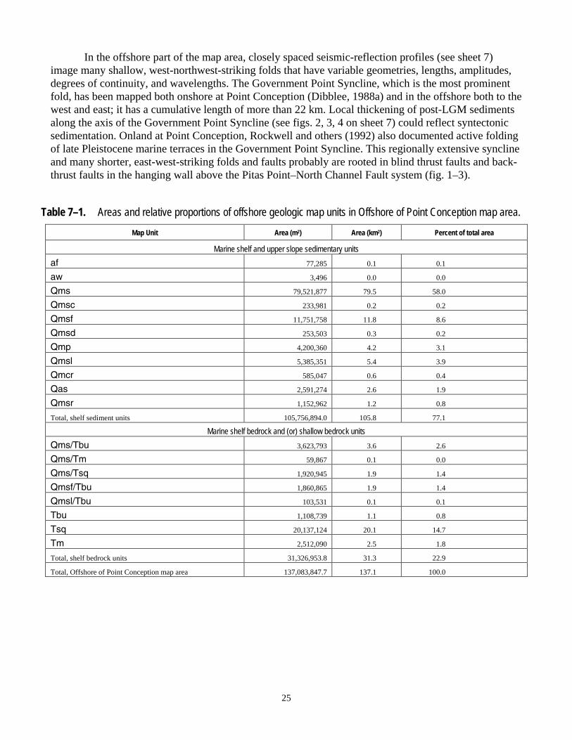
25

In the offshore part of the map area, closely spaced seismic-reflection profiles (see sheet 7) image many shallow, west-northwest-striking folds that have variable geometries, lengths, amplitudes, degrees of continuity, and wavelengths. The Government Point Syncline, which is the most prominent fold, has been mapped both onshore at Point Conception (Dibblee, 1988a) and in the offshore both to the west and east; it has a cumulative length of more than 22 km. Local thickening of post-LGM sediments along the axis of the Government Point Syncline (see figs. 2, 3, 4 on sheet 7) could reflect syntectonic sedimentation. Onland at Point Conception, Rockwell and others (1992) also documented active folding of late Pleistocene marine terraces in the Government Point Syncline. This regionally extensive syncline and many shorter, east-west-striking folds and faults probably are rooted in blind thrust faults and back- thrust faults in the hanging wall above the Pitas Point–North Channel Fault system (fig. 1–3).

Table 7–1. Areas and relative proportions of offshore geologic map units in Offshore of Point Conception map area.

Map Unit Area (m2) Area (km2) Percent of total area

Marine shelf and upper slope sedimentary units

af 77,285 0.1 0.1

aw 3,496 0.0 0.0

Qms 79,521,877 79.5 58.0

Qmsc 233,981 0.2 0.2

Qmsf 11,751,758 11.8 8.6

Qmsd 253,503 0.3 0.2

Qmp 4,200,360 4.2 3.1

Qmsl 5,385,351 5.4 3.9

Qmcr 585,047 0.6 0.4

Qas 2,591,274 2.6 1.9

Qmsr 1,152,962 1.2 0.8

Total, shelf sediment units 105,756,894.0 105.8 77.1

Marine shelf bedrock and (or) shallow bedrock units

Qms/Tbu 3,623,793 3.6 2.6

Qms/Tm 59,867 0.1 0.0

Qms/Tsq 1,920,945 1.9 1.4

Qmsf/Tbu 1,860,865 1.9 1.4

Qmsl/Tbu 103,531 0.1 0.1

Tbu 1,108,739 1.1 0.8

Tsq 20,137,124 20.1 14.7

Tm 2,512,090 2.5 1.8

Total, shelf bedrock units 31,326,953.8 31.3 22.9

Total, Offshore of Point Conception map area 137,083,847.7 137.1 100.0

26

DESCRIPTION OF MAP UNITS

OFFSHORE GEOLOGIC AND GEOMORPHIC UNITS

[Note that, where older units (typically, bedrock) are overlain by thin (<1 m thick) unconsolidated Quaternary deposits, composite units are mapped. These composite units, which are shown with gray, white, or black stipple pattern on older unit, are designated by composite label indicating both overlying sediment cover and lower (older) unit, separated by a slash (for example, Qms/Tm indicates that thin sheet of Qms overlies Tm)]

af Artificial seafloor (late Holocene)—Pipelines west of Point Conception; associated with offshore oil platforms

ass Artificially modified seafloor (late Holocene)—Shipwreck(?) Qms Marine nearshore and shelf deposits (late Holocene)—Mostly sand; ripples common.

Found on gently seaward-dipping (about 0.7° to 1.1°) surface that extends from nearshore to water depths of as much as about 85 m

Qmsc Coarse-grained marine nearshore and shelf deposits (late Holocene)—Ranges from coarse sand and gravel to boulders. Found as southwest-trending lens about 650 m south of Point Conception, at depths of 15 to 40 m, and along margins of seafloor bedrock outcrops between Point Conception and Point Arguello, at depths of about 30 to 50 m

Qmsf Fine-grained marine shelf deposits (late Holocene)—Mostly clay, silt, and very fine sand; commonly bioturbated; found on outer shelf, at water depths of more than about 85 m

Qmsd Marine shelf scour depressions (late Holocene)—Inferred to be coarse sand and possibly gravel, in low-relief scour depressions; found as single depressions or in groups of depressions interspersed with elevated shelf sediments (unit Qms) adjacent to seafloor bedrock outcrops, at water depths of about 15 to 40 m. Acoustic-backscatter data show intensity contrasts that suggest depressions are filled with sediment that is coarser than bounding elevated, sandy shelf deposits. Areas in which unit is found are not likely to change substantially, but boundaries of unit(s) and locations of individual depressions (and intervening flat sheets) likely are ephemeral, prone to change during significant storm events

Qmsr Marine shelf sand ridges (late Holocene)—Field (about 1.15 km2) of low-relief sand ridges and intervening troughs about 1.5 to 3.0 km south of Point Conception, at water depths of 65 to 80 m. Crests of sand ridges trend northeast (~60° azimuth), are as much as 750 m long, are spaced at intervals of about 125 to 200 m, and have heights of as much as 60 cm

Qmsl Marine upper slope deposits (Holocene)—Predominantly clay, silt, and very fine sand; commonly bioturbated. Found below shelf break on seaward-dipping (about 2.5°) surface, at water depths of more than about 100 m

Qmcr Marine slope canyons and rills (Holocene)—Probably sand and mud; forms incised trough, about 20 to 30 m deep and 600 m wide, into shelf break and outer shelf southwest of Point Conception; one of five heads of informally named Arguello canyon (Greene and others, 1991)

Qmp Marine pockmarks (Holocene)—Sand and mud, in circular to elliptical pockmarks. Pockmarks are solitary or grouped, and they range in size from 50 to 150 m on their long axis; they typically are 20 to 40 cm deep and ringed with convex rim as high as 150 cm

27

Qas Asphalt deposits (Holocene)—Asphalt (tar) mounds, probably mixed with sediment; weathered and biodegraded oil derived from underlying or nearby natural hydrocarbon seeps. Largest mounds cover 675,856 m2 and 168,950 m2 and have as much as about 12 m of relief above seafloor

Tbu Bedrock, undivided (Pliocene and Miocene)—Mainly mudstone and siltstone. Probably consists of the lower Pliocene and upper Miocene Sisquoc Formation and the Miocene Monterey Formation. Stippled areas are composite units where thin sheets of sediment (either Qms, Qmsf, or Qmsl) overlie bedrock: gray stipple indicates composite unit Qms/Tbu; white stipple, composite unit Qmsf/Tbu; and black stipple, composite unit Qmsl/Tbu

Tsq Sisquoc Formation (early Pliocene and late Miocene)—Marine, tan- to white-weathering, diatomaceous mudstone and shale, conglomerate, and subordinate dolomite. Stippled areas (composite unit Qms/Tsq) indicate where thin sheets of Qms overlie unit

Tm Monterey Formation (Miocene)—Predominantly well-bedded, siliceous and calcareous mudstone and shale. Stippled areas (composite unit Qms/Tm) indicate where thin sheets of Qms overlie unit

ONSHORE GEOLOGIC AND GEOMORPHIC UNITS

[Units compiled and modified from Dibblee (1988a,b); unit ages, which are from these sources, reflect local stratigraphic relations. In addition, some Quaternary units modified by C.W. Davenport on basis of analysis of 2004 ifSAR and 2009 lidar imagery]

af Artificial fill (late Holocene)—Engineered and (or) nonengineered material deposited by humans

Qb Beach deposits (late Holocene)—Unconsolidated, loose, fine- to coarse-grained sand, pebbles, and boulders; well sorted. Mapped in coastal band from shoreline to highest elevation of swash zone; may consist of thin veneer over bedrock platform

Qsc Active stream-channel deposits (late Holocene)—Active stream channels that contain unconsolidated sand, silt, and gravel deposits

Qd Dune-sand deposits (late Holocene)—Very well sorted, fine to medium sand; forms active dunes along coast

Qal Alluvial deposits, undivided (Holocene)—Sand, gravel, and silt deposits, adjacent to or near active stream channels. Locally, may include stream-terrace and -channel deposits too small to delineate at map scale

Qyf Alluvial fan deposits (Holocene)—Unconsolidated, heterogeneous layers of sand, silt, and gravel; relatively undissected; deposited by streams emanating from canyons onto alluvial plains; identified primarily by fan morphology and topographic expression. Internal contacts delineate individual alluvial fans

Qc Colluvium (Holocene)—Loose to firm, unsorted sand, silt, clay, gravel, rock debris, and organic material; includes slope wash and valley fill; may contain numerous small landslides and (or) coalesced alluvial fans

Qls Landslide deposits (Holocene and Pleistocene)—Deposits of diverse slope-movement processes; ranges from poorly sorted, disrupted mixtures of rock fragments and soil to relatively intact bedrock slump blocks; queried where identity is uncertain. Internal contacts delineate individual landslide bodies

Qa Alluvial deposits, undivided (Holocene and Pleistocene)—Sand, gravel, and silt deposits. Mapped on gently sloping to level surfaces near stream channels, where relative ages are uncertain or where separate units could not be delineated at map scale

28

Qf Alluvial fan deposits (Holocene and Pleistocene)—Poorly consolidated silt, sand, and gravel deposits. Mapped either where older age is indicated by greater degree of dissection or where elevations are higher than that of adjacent Holocene alluvial fans

Qof Alluvial fan deposits (Pleistocene)—Discontinuous or highly dissected deposits of semiconsolidated, moderately to poorly sorted layers of silty clay, silt, sand, and gravel

Qmt Marine-terrace deposits, undivided (Pleistocene)—Semiconsolidated sand and local gravel deposits; on uplifted marine-abrasion platforms along coast; locally, may include fluvial and (or) colluvial deposits too small to delineate at map scale

Tsq Sisquoc Formation (early Pliocene and late Miocene)—Marine shale, claystone, and diatomite; queried where identity is uncertain

Tm Monterey Formation, undivided (Miocene)—Marine, predominantly well-bedded, siliceous chert, mudstone, shale, diatomite, and conglomerate breccia. Locally divided into three subunits that are distinguished by stratigraphic position, lithology, and (or) age

Tmc Chert (Miocene) Tml Light-gray diatomite (Miocene) Tmls Semisiliceous shale (Miocene) Tt Tranquillon Volcanics (Miocene)—Rhyolitic tuff breccia Tr Rincon Shale (early Miocene)—Marine shale or claystone; queried where identity is

uncertain Tv Vaqueros Formation (late Oligocene)—Marine calcareous sandstone. Includes one subunit Tvsc Sandstone and pebble conglomerate (late Oligocene)—Queried where identity is

uncertain Ta Alegria Formation (Oligocene)—Marine, arkosic sandstone and greenish-gray siltstone;

locally fossiliferous (Dibblee, 1988a) Tg Gaviota Formation (Oligocene and Eocene)—Marine arkosic sandstone, locally

fossiliferous. Includes one subunit Tgs Concretionary siltstone and claystone (Oligocene and Eocene) Ts Sacate Formation (Eocene)—Marine arkosic sandstone that contains interbeds of

micaceous, clayey shale Tcd Cozy Dell Shale (Eocene)—Marine micaceous shale Tma Matilija Sandstone (Eocene)—Marine arkosic sandstone Tan Anita Shale (Eocene and Paleocene)—Marine, micaceous, clayey shale; includes

foraminiferal claystone (informally known as “Poppin shale”); queried where identity is uncertain. Also includes one mappable subunit

Tasb Sierra Blanca limestone (Eocene and Paleocene)—Algal limestone lens Kja Jalama Formation (Late Cretaceous)—Marine arkosic sandstone; includes three subunits Kjsl Siltstone (Late Cretaceous) Kjsh Micaceous shale and siltstone (Late Cretaceous) Kjss Arkosic sandstone and interbeds of micaceous shale (Late Cretaceous)

29

Acknowledgments

This publication was funded by the California Ocean Protection Council and the U.S. Geological Survey (USGS) Coastal and Marine Geology Program. We thank Robert Garrison and Hilde Schwartz (both University of California, Santa Cruz) for their critical reviews that greatly improved this report. We are grateful to USGS editor Taryn Lindquist for helping us develop the templates and formats for this series of publications, and for invaluable editorial review and suggestions.

30

References Cited

Blanchette, C.A., Helmuth, B., and Gaines, S.D., 2007, Spatial patterns of growth in the mussel, Mytilus californianus, across a major oceanographic and biogeographic boundary at Point Conception, California, USA: Journal of Experimental Marine Biology and Ecology, v. 340, p. 126–148.

Briggs, J.C., 1974, Marine zoogeography: New York, McGraw-Hill, 480 p. Brink, K.H., and Muench, R.D., 1986, Circulation in the Point Conception–Santa Barbara Channel

region: Journal of Geophysical Research, v. 91, p. 877–895. Cacchione, D.A., Drake, D.E., Grant, W.D., and Tate, G.B., 1984, Rippled scour depressions of the

inner continental shelf off central California: Journal of Sedimentary Petrology, v. 54, p. 1,280–1,291. California Department of Fish and Wildlife, 2008, California Marine Life Protection Act master plan for

marine protected areas—Revised draft: California Department of Fish and Wildlife [formerly California Department of Fish and Game], available at https://www.wildlife.ca.gov/Conservation/ Marine/MPAs/Master-Plan.

California State University, Monterey Bay, Seafloor Mapping Lab, 2016, Southern California 2008 CSMP surveys: California State University, Monterey Bay, Seafloor Mapping Lab Data Library, accessed October 2016 at http://seafloor.otterlabs.org/SFMLwebDATA_SURVEYMAP.htm.

Chaytor, J.D., Goldfinger, C., Meinter, M.A., Huftile, G.J., Rosmos, C.G., and Legg, M.R., 2008, Measuring vertical tectonic motion at the intersection of the Santa Cruz-Santa Catalina Ridge and Northern Channel Islands platform, California Continental Borderland, using submerged paleoshorelines: Geological Society of America Bulletin, v. 120, p. 1,053–1,071.

Cochrane, G.R., 2008, Video-supervised classification of sonar data for mapping seafloor habitat, in Reynolds, J.R., and Greene, H.G., eds., Marine habitat mapping technology for Alaska: Fairbanks, University of Alaska, Alaska Sea Grant College Program, p. 185–194, available at http://doc.nprb.org/ web/research/research%20pubs/615_habitat_mapping_workshop/Individual%20Chapters%20High- Res/Ch13%20Cochrane.pdf.

Cochrane, G.R., Conrad, J.E., Reid, J.A., Fangman, S., and Golden, N., 2005, Nearshore benthic habitat GIS for the Channel Islands National Marine Sanctuary and southern California state fisheries reserves, vol. II: U.S. Geological Survey Open-File Report 2005–1170, available at https://pubs.usgs.gov/of/2005/1170/.

Cochrane, G.R., Nasby, N.M., Reid, J.A., Waltenberger, B., and Lee, K.M., 2003, Nearshore benthic habitat GIS for the Channel Islands National Marine Sanctuary and southern California state fisheries reserves, vol. I: U.S. Geological Survey Open-File Report 03–85, available at https://pubs.usgs.gov/of/2003/0085/.

Cudaback, C.N., Washburn, L., and Dever, E., 2005, Subtidal inner-shelf circulation near Point Conception, California: Journal of Geophysical Research, v. 110, C10007, available at https://doi.org/10.1029/2004JC002608.

Davis, A.C.D., Kvitek, R.G., Mueller, C.B.A., Young, M.A., Storlazzi, C.D., and Phillips, E.L., 2013, Distribution and abundance of rippled scour depressions along the California coast: Continental Shelf Research, v. 69, p. 88–100, available at https://doi.org/10.1016/j.csr.2013.09.010.

Dibblee, T.W., Jr., 1988a, Geologic map of the Lompoc Hills and Point Conception quadrangles, Santa Barbara County, California (H.E. Ehrenspeck [1988] and J.A. Minch [2009], eds.): Dibblee Geological Foundation Map DF-18, scale 1:24,000.

Dibblee, T.W., Jr., 1988b, Geologic map of the Point Arguello and Tranquillon Mountain quadrangles, Santa Barbara County, California (H.E. Ehrenspeck [1988] and J.A. Minch [2009], eds.): Dibblee Geological Foundation Map DF-19, scale 1:24,000.

Draut, A.E., Hart, P.E., Lorenson, T.D., Ryan, H.F., Wong, F.L., Sliter, R.W., and Conrad, J.E., 2009, Late Pleistocene to Holocene sedimentation and hydrocarbon seeps on the continental shelf of a steep,

31

tectonically active margin, southern California, USA: Marine Geophysical Research, p. 193–206, available at https://doi.org/10.1007/s11001-009-9076-y.

Duvall, A., Kirby, E., and Burbank, D., 2004, Tectonic and lithologic controls on bedrock channel profiles and processes in coastal California: Journal of Geophysical Research, v. 109, 18 p., F03002, available at https://doi.org/10.1029/2003JF000086,2004.

Eichhubl, P., Greene, H.G., and Maher, N., 2002, Physiography of an active transpressive margin basin—High-resolution bathymetry of the Santa Barbara basin, southern California continental borderland: Marine Geology, v. 184, p. 95–120.

Fader, G.B.J., 1997, Effects of shallow gas on seismic-reflection profiles, in Davies, T.A., Bell, T., Cooper, A.K., Josenhaus, H., Polyak, L., Solheim, A., Stoker, M.S., and Stravers, J.A., eds., Glaciated continental margins—An atlas of acoustic images: London, Chapman & Hall, p. 29–30.

Fischer, P.J., 1998, Structure and tectonics of northwestern Santa Barbara basin, in Kunitomi, D.S., Hopps, T.E., and Galloway, J.M., eds., Structure and petroleum geology, Santa Barbara Channel, California: American Association of Petroleum Geologists, Pacific Section, and Coast Geological Society, Miscellaneous Publication 46, p, 79–96.

Fisher, M.A., Sorlien, C.C., and Sliter, R.W., 2009, Potential earthquake faults offshore southern California from the eastern Santa Barbara channel to Dana Point, in Lee, H.J., and Normark, W.R., eds., Earth science in the urban ocean—The Southern California Continental Borderland: Geological Society of America Special Paper 454, p. 271–290.

Galloway, J.M., 1998, Chronology of petroleum exploration and development in the Santa Barbara channel area, offshore southern California, in Kunitomi, D.S., Hopps, T.E., and Galloway, J.M., eds., Structure and petroleum geology, Santa Barbara Channel, California: American Association of Petroleum Geologists, Pacific Section, and Coast Geological Society, Miscellaneous Publication 46, p. 1–12, 1 sheet.

Goff, J.A., Mayer, L.A., Traykovski, P., Buynevich, I., Wilkens, R., Raymond, R., Glang, G., Evans, R.L., Olson, H., and Jenkins, C., 2005, Detailed investigations of sorted bedforms or “rippled scour depressions,” within the Martha’s Vineyard Coastal Observatory, Massachusetts: Continental Shelf Research, v. 25, p. 461–484.

Golden, N.E., and Cochrane, G.R., 2013, California Seafloor Mapping Program video and photograph portal: U.S. Geological Survey, Coastal and Marine Geology Program data portal, available at https://doi.org/10.5066/F7J1015K.

Greene, H.G., and Bizzarro, J.J., 2003, Essential fish habitat characterization and mapping of the California continental margin: Final Report to Pacific States Marine Fisheries Commission, CFDA #11-454, 14 p., available at http://marinehabitat.psmfc.org/files/source_docs/ EFH_report_with_Appendices.pdf.

Greene, H.G., Bizzarro, J.J., O’Connell, V.M., and Brylinsky, C.K., 2007, Construction of digital potential marine benthic habitat maps using a coded classification scheme and its application, in Todd, B.J., and Greene, H.G., eds., Mapping the seafloor for habitat characterization: Geological Association of Canada Special Paper 47, p. 141–155.

Greene, H.G., Clarke, S.H., Jr., and Kennedy, M.P., 1991, Tectonic evolution of submarine canyons along the California continental margin, in Osborne, R.H., ed., From shoreline to abyss: Society for Sedimentary Geology Special Publication 46, p. 231–248.

Greene, H.G., Yoklavich, M.M., Starr, R.M., O’Connell, V.M., Wakefield, W.W., Sullivan, D.E., McRea, J.E., and Cailliet, G.M., 1999, A classification scheme for deep seafloor habitats: Oceanologica Acta, v. 22, p. 663–678.

Griggs, G., Patsch, K., and Savoy, L., 2005, Living with the changing California coast: Berkeley, University of California Press, 540 p.

32

Gurrola, L.D., Keller, E.A., Chen, J.H., Owen, L.A., and Spencer, J.Q., 2014, Tectonic geomorphology of marine terraces—Santa Barbara fold belt, California: Geological Society of America Bulletin, v. 126, p. 219–233.

Hallenbeck, T.R., Kvitek, R.G., and Lindholm, J., 2012, Rippled scour depressions add ecologically significant heterogeneity to soft-bottom habitats on the continental shelf: Marine Ecology Progress Series, v. 468, p. 119–133, available at https://doi.org/10.3354/meps09948.

Hapke, C.J., and Reid, D.R., 2007, National assessment of shoreline change, part 4—Historical coastal cliff retreat along the California Coast: U.S. Geological Survey Open-File Report 2007–1133, 51 p., available at http://pubs.usgs.gov/of/2007/1133/.

Hapke, C.J., Reid, D., Richmond, B.B., Ruggiero, P., and List, J., 2006, National assessment of shoreline change, part 3—Historical shoreline change and associated coastal land loss along sandy shorelines of the California coast: U.S. Geological Survey Open-File Report 2006–1219, 72 p., available at http://pubs.usgs.gov/of/2006/1219/.

Hornafius, J.S., Luyendyk, B.P., Terres, R.R., and Kamerling, M.J., 1986, Timing and extent of Neogene rotation in the western Transverse Ranges, California: Geological Society of America Bulletin, v. 97, p. 1,476–1,487.

Hovland, M., and Judd, A.G., 1988, Seabed pockmark and seepages: London, Graham and Trotman, Inc., 293 p.

Jennings, C.W., and Bryant, W.A., 2010, Fault activity map of California: California Geological Survey Geologic Data Map no. 6, scale 1:750,000, available at http://www.conservation.ca.gov/cgs/ cgs_history/Pages/2010_faultmap.aspx.

Johnson, S.Y., Cochrane, G.R., Golden, N.E., Dartnell, P., Hartwell, S.R., Cochran, S.A., and Watt, J.T., 2017a, The California Seafloor and Coastal Mapping Program—Providing science and geospatial data for California’s State Waters: Ocean and Coastal Management, v. 140, p. 88–104, available at https://doi.org/10.1016/j.ocecoaman.2017.02.004.

Johnson, S.Y., Dartnell, P., Cochrane, G.R., Golden, N.E., Phillips, E.L., Ritchie, A.C., Greene, H.G., Krigsman, L.M., Kvitek, R.G., Dieter, B.E., Endris, C.A., Seitz, G.G., Sliter, R.W., Erdey, M.E., Gutierrez, C.I., Wong, F.L., Yoklavich, M.M., Draut, A.E., Hart, P.E., and Conrad, J.E. (S.Y. Johnson and S.A. Cochran, eds.), 2013a, California State Waters Map Series—Offshore of Santa Barbara, California: U.S. Geological Survey Scientific Investigations Map 3281, pamphlet 45 p., 11 sheets, scale 1:24,000, available at https://doi.org/10.3133/sim3281.

Johnson, S.Y., Dartnell, P., Cochrane, G.R., Golden, N.E., Phillips, E.L., Ritchie, A.C., Krigsman, L.M., Dieter, B.E., Conrad, J.E., Greene, H.G., Seitz, G.G., Endris, C.A., Sliter, R.W., Wong, F.L., Erdey, M.D., Gutierrez, C.I., Yoklavich, M.M., East, A.E., and Hart, P.E. (S.Y. Johnson and S.A. Cochran, eds.), 2015, California State Waters Map Series—Offshore of Refugio Beach, California: U.S. Geological Survey Scientific Investigations Map 3319, pamphlet 42 p., 11 sheets, scale 1:24,000, available at https://doi.org/10.3133/sim3319.

Johnson, S.Y., Dartnell, P., Cochrane, G.R., Golden, N.E., Phillips, E.L., Ritchie, A.C., Kvitek, R.G., Dieter, B.E., Conrad, J.E., Lorenson, T.D., Krigsman, L.M., Greene, H.G., Endris, C.A., Seitz, G.G., Finlayson, D.P., Sliter, R.W., Wong, F.L., Erdey, M.D., Gutierrez, C.I., Leifer, I., Yoklavich, M.M., Draut, A.E., Hart, P.E., Hostettler, F.D., Peters, K.E., Kvenvolden, K.A., Rosenbauer, R.J., and Fong, G. (S.Y. Johnson and S.A. Cochran, eds.), 2014, California State Waters Map Series—Offshore of Coal Oil Point, California: U.S. Geological Survey Scientific Investigations Map 3302, pamphlet 57 p., 12 sheets, scale 1:24,000, available at https://doi.org/10.3133/sim3302.

Johnson, S.Y., Dartnell, P., Cochrane, G.R., Golden, N.E., Phillips, E.L., Ritchie, A.C., Kvitek, R.G., Greene, H.G., Endris, C.A., Seitz, G.G., Sliter, R.W., Erdey, M.D., Wong, F.L., Gutierrez, C.I., Krigsman, L.M., Draut, A.E., and Hart, P.E. (S.Y. Johnson and S.A. Cochran, eds.), 2013c, California

33

State Waters Map Series—Offshore of Carpinteria, California: U.S. Geological Survey Scientific Investigations Map 3261, pamphlet 42 p., 10 sheets, available at http://pubs.usgs.gov/sim/3261/.

Johnson, S.Y., Dartnell, P., Cochrane, G.R., Golden, N.E., Phillips, E.L., Ritchie, A.C., Kvitek, R.G., Greene, H.G., Krigsman, L.M., Endris, C.A., Clahan, K.B., Sliter, R.W., Wong, F.L., Yoklavich, M.M., and Normark, W.R. (S.Y. Johnson, ed.), 2012, California State Waters Map Series—Hueneme Canyon and vicinity, California: U.S. Geological Survey Scientific Investigations Map 3225, pamphlet 41 p., 12 sheets, scale 1:24,000, available at http://pubs.usgs.gov/sim/3225/.

Johnson, S.Y., Dartnell, P., Cochrane, G.R., Golden, N.E., Phillips, E.L., Ritchie, A.C., Kvitek, R.G., Greene, H.G., Krigsman, L.M., Endris, C.A., Seitz, G.G., Gutierrez, C.I., Sliter, R.W., Erdey, M.D., Wong, F.L., Yoklavich, M.M., Draut, A.E., and Hart, P.E. (S.Y. Johnson and S.A. Cochran, eds.), 2013b, California State Waters Map Series—Offshore of Ventura, California: U.S. Geological Survey Scientific Investigations Map 3254, pamphlet 42 p., 11 sheets, scale, 1:24,000, available at http://pubs.usgs.gov/sim/3254/.

Johnson, S.Y., Dartnell, P., Cochrane, G.R., Hartwell, S.R., Golden, N.E., Kvitek, R.G., and Davenport, C.W. (S.Y. Johnson and S.A. Cochran, eds.), 2018, California State Waters Map Series—Offshore of Gaviota, California: U.S. Geological Survey Open-File Report 2018–1023, pamphlet 41 p., 9 sheets, scale 1:24,000, available at https://doi.org/10.3133/ofr20181023.

Johnson, S.Y., Hartwell, S.R., and Beeson, J.W., 2016, Marine geophysical data—Point Sal to Refugio State Beach, southern California: U.S. Geological Survey data release, available at https://doi.org/10.5066/F7SX6BCD.

Johnson, S.Y., Hartwell, S.R., Sorlien, C.C., Dartnell, P., and Ritchie, A.R., 2017b, Shelf evolution along a transpressive transform margin, Santa Barbara Channel, California: Geosphere, v. 13, p. 2,041–2,077.

Keller, E.A., Duffy, M., Kennett, J.P., and Hill, T., 2007, Tectonic geomorphology and hydrocarbon- induced topography of the mid-Channel anticline, Santa Barbara basin, California: Geomorphology, v. 89, p. 274–286.

Kunitomi, D.S., Hopps, T.E., and Galloway, J.M., eds., 1998, Structure and petroleum geology, Santa Barbara Channel, California: American Association of Petroleum Geologists, Pacific Section, and Coast Geological Society, Miscellaneous Publication 46, 328 p.

Kvitek, R., Bretz, C., Cochrane, G.R., and Greene, H.G., 2006, Final report, Statewide Marine Mapping Planning Workshop, December 12–13, 2005, Seaside, Calif.: California State University, Monterey Bay, 108 p., available at http://www.opc.ca.gov/webmaster/ftp/project_pages/mapping/2005 FINAL mapping report April 2006.pdf.

Kvitek, R.G., Phillips, E.L., and Dartnell, P., 2012, Colored shaded-relief bathymetry, Hueneme Canyon and vicinity, California, sheet 1 in Johnson, S.Y., Dartnell, P., Cochrane, G.R., Golden, M.E., Phillips, E.L., Ritchie, A.C., Kvitek, R.G., Greene, H.G., Krigsman, L.M., Endris, C.A., Clahan, K.B., Sliter, R.W., Wong, F.L., Yoklavich, M.M., and Normark, W.R. (S.Y. Johnson, ed.), California State Waters Map Series—Hueneme Canyon and vicinity, California: U.S. Geological Survey Scientific Investigations Map 3225, pamphlet 41 p., 12 sheets, available at http://pubs.usgs.gov/sim/3225/.

Larson, K.M., and Webb, F.H., 1992, Deformation in the Santa Barbara Channel from GPS measurements 1987–1991: Geophysical News Letters, v. 19, p. 1,491–1,494.

Lee, H.J., and Normark, W.R., eds., 2009, Earth science in the urban ocean—The Southern California Continental Borderland: Geological Society of America Special Paper 454, 481 p.

Lee, W.H.K., and Vedder, J.G., 1973, Recent earthquake activity in the Santa Barbara Channel region: Bulletin of the Seismological Society of America, v. 63, p. 1,757–1,773.

Lorenson, T.D, Hostettler, F.D., Rosenbauer, R.J., Peters, K.E., Kvenvolden, K.A., Dougherty, J.A., Gutmacher, C.E., Wong, F.L., and Normark, W.R., 2009, Natural offshore seepage and related tarball accumulation on the California coastline, Santa Barbara Channel and the southern Santa Maria

34

Basin—Source identification and inventory: U.S. Geological Survey Open-File Report 2009–1225 [also released as Minerals Management Service Report 2009–030], 116 p., available at http://pubs.usgs.gov/of/2009/1225/.

Lorenson, T.D., Wong, F.L., Dartnell, P., and Sliter, R.W., 2014, Greenhouse gases generated from the anaerobic biodegradation of natural offshore asphalt seepages in southern California: Geo-Marine Letters, v. 34, p. 281–295, available at https://doi.org/10.1007/s00367-014-0359-1/.

Luyendyk, B.P., Kamerling, M.J., and Terres, R.R., 1980, Geometric model for Neogene crustal rotations in southern California: Geological Society of America Bulletin, v. 91, p. 211–217.

Madden, C.J., Goodin, K.L., Allee, R., Finkbeiner, M., and Bamford, D.E., 2008, Draft Coastal and Marine Ecological Classification Standard: National Oceanic and Atmospheric Administration (NOAA) and NatureServe, v. III, 77 p.

Marshall, S.T., Funning, G.J., and Owen, S.E., 2013, Fault slip rates and interseismic deformation in the western Transverse Ranges, California: Journal of Geophysical Research, v. 118, 24 p., available at https://doi.org/10.1002/jgrb.50312.

Metcalf, J.G., 1994, Morphology, chronology, and deformation of Pleistocene marine terraces, southwestern Santa Barbara County, Santa Barbara, California: Santa Barbara, University of California, M.S. thesis, 168 p.

Minor, S.A., Kellogg, K.S., Stanley, R.G., Gurrola, L.D., Keller, E.A., and Brandt, T.R., 2009, Geologic map of the Santa Barbara coastal plain area, Santa Barbara County, California: U.S. Geological Survey Scientific Investigations Map 3001, scale 1:25,000, 1 sheet, pamphlet 38 p., available at http://pubs.usgs.gov/sim/3001/.

Mitchum, R.M., Jr., Vail, P.R., and Sangree, J.B., 1977, Seismic stratigraphy and global changes of sea level, part 6—Stratigraphic interpretation of seismic reflection patterns in depositional sequences, in Payton, C.E., ed., Seismic stratigraphy—Applications to hydrocarbon exploration: Tulsa, Okla., American Association of Petroleum Geologists, p. 117–133.

Monterey Bay Aquarium Research Institute, 2002, Santa Barbara multibeam survey: Monterey Bay Aquarium Research Institute Digital Data Series 4, 2 CD-ROMs.

Muhs, D.R., Rockwell, T.K., and Kennedy, G.L., 1992, Late Quaternary uplift rates of marine terraces on the Pacific Coast of North America, southern Oregon to Baja California Sur: Quaternary International, v. 15/16, p. 121–133.

Murray, A.B., and Thieler, E.R., 2004, A new hypothesis and exploratory model for the formation of large-scale inner-shelf sediment sorting and “rippled scour depressions:” Continental Shelf Research, v. 24, no. 3, p. 295–315.

National Geodetic Survey, 2016, NOAA Shoreline Data Explorer: National Oceanic and Atmospheric Administration, National Geodetic Survey data viewer and database, accessed May 1, 2016, at http://www.ngs.noaa.gov/NSDE/.

National Oceanic and Atmospheric Administration, 2013, 2013 NOAA Coastal California TopoBathy Merge Project: National Oceanic and Atmospheric Administration, National Centers for Environmental Information database, accessed August 2016 at http://www.ngdc.noaa.gov/docucomp/ page?xml=NOAA/NESDIS/NGDC/MGG/Lidar/iso/xml/2013_CA_TopoBathy_m2612.xml&view=ge tDataView&header=none.

Nicholson, C., Sorlien, C., Atwater, T., Crowell, J.C., and Luyendyk, B.P., 1994, Microplate capture, rotation of the western Transverse Ranges, and initiation of the San Andreas transform as a low-angle fault system: Geology, v. 22, p. 491–495.

Peltier, W.R., and Fairbanks, R.G., 2006, Global glacial ice volume and Last Glacial Maximum duration from an extended Barbados sea level record: Quaternary Science Reviews, v. 25, p. 3,322–3,337.

Petersen, M.D., Moschetti, M.P., Powers, P.M., Mueller, C.S., Haller, K.M., Frankel, A.D., Zeng, Y., Rezaeian, S., Harmsen, S.C., Boyd, O.S., Field, N., Chen, R., Rukstales, K.S., Luco, N., Wheeler,

35

R.L., Williams, R.A., and Olsen, A.H., 2014, Documentation for the 2014 update of the United States national seismic hazard maps: U.S. Geological Survey Open-File Report 2014–1091, 243 p., available at https://doi.org/10.3133/ofr20141091.

Redin, T., Forman, J., Kamerling, M., and Galloway, J., 2005, Santa Barbara Channel structure and correlation sections—CS-32 to CS-42: American Association of Petroleum Geologists, Pacific Section, Publication CS 36, 12 sheets.

Reid, J.A., Reid, J.M., Jenkins, C.J., Zimmerman, M., Williams, S.J., and Field, M.E., 2006, usSEABED—Pacific Coast (California, Oregon, Washington) offshore surficial-sediment data release: U.S. Geological Survey Data Series 182, available at http://pubs.usgs.gov/ds/2006/182/.

Rockwell, T.K., Nolan, J., Johnson, D.L., and Patterson, R.H., 1992, Ages and deformation of marine terraces between Point Conception and Gaviota, Western Transverse Ranges, California, in Wehmiller, J.F., and Fletcher, C., eds., Quaternary coasts of the United States—Marine and lacustrine systems: Society of Economic Paleontologists and Mineralogists, p. 333–341.

Sorlien, C.C., Kamerling, M.J., Seeber, L., and Broderick, K.G., 2006. Restraining segments and reactivation of the Santa Monica–Dume–Malibu Coast fault system, offshore Los Angeles, California: Journal of Geophysical Research, Solid Earth, v. 11, 22 p.

Sorlien, C.C., and Nicholson, C., 2015, Post 1-Ma deformation history of the Pitas Point-North Channel- Red Mountain fault system and associated folds in Santa Barbara channel, California: U.S. Geological Survey National Earthquake Hazards Reduction Program final report, Award G14AP00012, 24 p., available at https://earthquake.usgs.gov/cfusion/external_grants/reports/G14AP00012.pdf.

Stanford, J.D., Hemingway, R., Rohling, E.J., Challenor, P.G., Medina-Elizalde, M., and Lester, A.J., 2011, Sea-level probability for the last deglaciation—A statistical analysis of far-field records: Global and Planetary Change, v. 79, p. 193–203, available at https://doi.org/10.1016/j.gloplacha.2010.11.002.

Stover, C.W., and Coffman, J.L., 1993, Seismicity of the United States, 1568-1989 (revised): U.S. Government Printing Office, 418 p.

Sylvester, A.G., 2001, Catalog of Santa Barbara earthquakes—1800 to 1960: Santa Barbara, University of California, Santa Barbara database, accessed March 2016 at http://projects.crustal.ucsb.edu/ sb_eqs/SBEQCatlog/SBEQCATINTRO.html.

Sylvester, A.G., Smith, S.S., and Scholz, C.H., 1970, Earthquake swarm in the Santa Barbara Channel, California, 1968: Bulletin of the Seismological Society of America, v. 60, p. 1,047–1,060.

Trembanis, A.C., and Hume, T.M., 2011, Sorted bedforms on the inner shelf off northeastern New Zealand—Spatiotemporal relationships and potential paleo-environmental implications: Geo-Marine Letters, v. 31, p. 203–214, available at https://doi.org/10.1007/s00367-010-0225-8.

Triezenberg, P.J., Hart, P.E., and Childs, J.R., 2016, National Archive of Marine Seismic Surveys (NAMSS)—A USGS data website of marine seismic reflection data within the U.S. Exclusive Economic Zone (EEZ): U.S. Geological Survey data release, accessed June 29, 2015, at https://doi.org/10.5066/F7930R7P [formerly U.S. Geological Survey’s National Archive of Marine Seismic Surveys database, available at http://walrus.wr.usgs.gov/NAMSS/].

U.S. Geological Survey, 2016, Earthquake catalog: U.S. Geological Survey database, accessed June 14, 2016, at https://earthquake.usgs.gov/earthquakes/search/.

U.S. Geological Survey and California Geological Survey, 2016, Quaternary fault and fold database of the United States: U.S. Geological Survey database, accessed April 5, 2016, at http://earthquake.usgs.gov/hazards/qfaults/.

Warrick, J.A., and Farnsworth, K.L., 2009, Sources of sediment to the coastal waters of the Southern California Bight, in Lee, H.J., and Normark, W.R., eds., Earth science in the urban ocean—The Southern California Continental Borderland: Geological Society of America Special Paper 454, p. 39– 52.

36

Warrick, J.A., and Mertes, L.A.K., 2009, Sediment yield from the tectonically active semiarid Western Transverse Ranges of California: Geological Society of America Bulletin, v. 121, p. 1,054–1,070.

Wong, F.L., Phillips, E.L., Johnson, S.Y, and Sliter, R.W., 2012, Modeling of depth to base of Last Glacial Maximum and seafloor sediment thickness for the California State Waters Map Series, eastern Santa Barbara Channel, California: U.S. Geological Survey Open-File Report 2012–1161, 16 p., available at http://pubs.usgs.gov/of/2012/1161/.

Wright, D.J., Pendleton, M., Boulware, J., Walbridge, S., Gerlt, B., Eslinger, D., Sampson, D., and Huntley, E., 2012, ArcGIS Benthic Terrain Modeler (BTM), v. 3.0: Environmental Systems Research Institute, NOAA Coastal Services Center, Massachusetts Office of Coastal Zone Management, accessed March 2016 at http://esriurl.com/5754.

Yerkes, R.F., Wagner, H.C., and Yenne, K.A., 1969, Petroleum development in the region of the Santa Barbara Channel: U.S. Geological Survey Professional Paper 679–B, p. 11–21.