Callable puts as composite exotic options∗

C. Kuhn† and A. E. Kyprianou‡

Abstract

Introduced by Kifer (2000), game options function in the same wayas American options with the added feature that the writer may alsochoose to exercise at which time they must pay out the intrinsic optionvalue of that moment plus a penalty. In Kyprianou (2004) an explicitformula was obtained for the value function of the perpetual put optionof this type. Crucial to the calculations which lead to the aforementionedformula was the perpetual nature of the option. In this article we addresshow to characterize the value function of the finite expiry version of thisoption via mixtures of other exotic options by using mainly martingalearguments.

Keywords: Game options, Dynkin games, fluctuation theory, local time.

JEL Classification: G13, C73.

Mathematics Subject Classification (2000): 91A15, 60G40, 35R35, 60J55.

1 Introduction

Consider the Black-Scholes market. That is, a market with a risky asset S anda riskless bond, B. The bond evolves according to the dynamic

dBt = rBtdt where r, t ≥ 0.

The risky asset is written as the process S = St : t ≥ 0 where

St = x expσWt + µt where x > 0

is the initial value of S and W = Wt : t ≥ 0 is a Brownian motion defined onthe filtered probability space (Ω,F , F = Ftt≥0, P ) satisfying the usual condi-tions and T ∈ (0,∞) is the time horizon. A callable put is an American putwith the additional feature that the seller can recall the option prematurelypaying besides the intrinsic value a constant penalty δ.

∗Both authors are grateful to two anonymous referees and the associate editor for extensiveconstructive remarks on an earlier version of this paper.

†Address: Frankfurt MathFinance Institute, Johann Wolfgang Goethe-Universitat, 60054Frankfurt a.M., Germany, e-mail: ckuehn@math.uni-frankfurt.de

‡Address: Department of Mathematical Sciences, THe University of Bath, Claverton Down,Bath BA2 7AY, UK, e-mail: a.kyprianou@bath.ac.uk

1

If the holder exercises first, (s)he may claim the value (K − St)+ at theexercise date and if the writer exercises prematurely, (s)he is obliged to payto the holder the value (K − St)+ + δ at the time of exercise. If neither havecanceled at time T then the writer pays the holder the value (K − ST )+. Ifboth decide to claim at the same time then the lesser of the two claims is paid(But, it turns out that the agreement about this marginal case has no impacton the resulting option price). Our objective in this paper is to characterizethe value and rational behaviour of writer and holder which lead to this value.However, before getting involved with technicalities, let us address the followingfundamental question.

Who should buy and who should sell a callable put ?

Assume that the option starts far out of the money, i.e. x K. If St

hits K (goes in the money) quite late, i.e. near to expiry, the risk for thewriter is comparatively small. By contrast, when St hits K quite early in theoption lifetime it becomes a long-term at-the-money-option which has a largetime value. Against this risky situation, the writer is insured by the right torecall the option. Put differently, by the callable feature the writer has an upperbound on the time value conceded to the put holder.

In the context of an illiquid market where the writer cannot compensateher/his short position by buying an American residual put option recalling ispossibly the only way to close the position. Also, in view of model risk orviolation of the hypothesis of market completeness, the cheapest superhedgingstrategy for the writer of an American put option can be the trivial one – consist-ing of an investment of K units in the riskless bank account. In this situation,strategic recalling can be an efficient instrument to limit risk – especially whenthe writer expects falling stock prices.

On the other hand for the buyer the incentive is the lower price (as it is forcallable bonds). This comes at the price that extreme gains become less likely.

A deposit insurance can be viewed as a callable perpetual put option on themarket value of the assets issued by the insured bank. The put writer – usuallya federal deposit insurer – agrees to purchase the bank’s insured deposits for themarket value of the bank’s assets (if the bank closes itself). On the other handthe deposit insurer can enfore premature exercise of the option by recalling theput option and closing the bank. For details, see Allen and Saunders (1993).

Returning now to the technical description of the callable put, let Tt,T be theclass of F-stopping times valued in [t, T ] and let Px be the risk-neutral measurefor S under the assumption that S0 = x. [Note that standard Black-Scholestheory dictates that this measure exists and is uniquely defined via a Girsanovchange of measure]. We shall denote Ex to be expectation under Px. From Kifer(2000) it follows that there is a unique no-arbitrage price process of the callableput under the Black-Scholes framework which can be represented by the right

2

continuous process V = Vt : t ∈ [0, T ] where

Vt = ess-infτ∈Tt,T ess-supσ∈Tt,TEx

(1(σ≤τ)e

−r(σ−t)(K − Sσ)+

+1(τ<σ)e−r(τ−t)

(K − Sτ )+ + δ

∣∣∣Ft

)= ess-supσ∈Tt,T

ess-infτ∈Tt,T Ex

(1(σ≤τ)e

−r(σ−t)(K − Sσ)+

+1(τ<σ)e−r(τ−t)

(K − Sτ )+ + δ

∣∣∣Ft

).

Further, for all t ∈ [0, T ] there exist stopping strategies

σ∗T−t = inf

s ∈ [t, T ] : Vs = (K − Ss)+

and

τ∗T−t = inf

s ∈ [t, T ] : Vs = (K − Ss)+ + 1(s<T )δ

. (1)

such that

Vt = Ex

(1(σ∗

T−t≤τ∗T−t)e

−r(σ∗T−t−t)(K − Sσ∗

T−t)+

+1(τ∗T−t<σ∗

T−t)e−r(τ∗

T−t−t)δ + (K − Sτ∗

T−t)+

∣∣∣Ft

)(2)

By the Markov property we can write Vt = vCP (St, T − t) where

vCP (x, u) = infτ∈T0,u

supσ∈T0,u

Ex

(1(σ≤τ)e

−rσ(K − Sσ)+

+1(τ<σ)e−rτ

(K − Sτ )+ + δ

)= sup

σ∈T0,u

infτ∈T0,u

Ex

(1(σ≤τ)e

−rσ(K − Sσ)++

1(τ<σ)e−rτ

(K − Sτ )+ + δ

)(3)

defined on (x, u) ∈ (0,∞) × [0, T ]. Note that by considering strategies σ = 0and τ = 0 it can be seen that

(K − x)+ ≤ vCP (x, u) ≤ (K − x)+ + δ. (4)

Our interest is in showing how the value function vCP (x, u) can be char-acterized in terms of the value functions of other more familiar exotic options.However it is first necessary to understand whether the writer’s rights reallymakes a significant difference to the case of the American put.

In Kyprianou (2004) for T = ∞ explicit formulae expressions are achieved forVt in terms of the process S. The calculations are greatly eased by the perpetualnature of the option. For the finite expiry version, no explicit formulae arepossible for the same reason that there are no explicit formulae for the valuefunction of an American put. In this article we establish representations of finiteexpiry versions of the callable put via mixtures of other familiar exotic options.The method of proof relies on the classical technique of ‘guess and verify’.

We close this section with an overview of the paper. Section 2 reviews theAmerican put for later reflection. For a suitably large value of δ, i.e. exceeding

3

a specified threshold, it turns out that the value of the callable put is nothingmore than the value of the American put. That is to say the writer will neverexercise. This is dealt with in Section 3. In Section 4 the more interestingand complicated case of when δ is smaller than the aforementioned threshold isconsidered. The paper presents its conclusions in Section 5.

2 Reviewing the American put

It will be of help to review some facts concerning the pricing of a regular Ameri-can put option (cf. Karatzas and Shreve (1998), Lamberton (1998) and Myneni(1992)). That is to say, a contract with finite expiry date T which rewards theholder with (K − St)+ at the moment they decide to exercise and forces a pay-ment of (K − ST )+ if they have not exercised by the time the contract expires.Classical analysis of the American put tells us that

Vt = ess-supσ∈Tt,TEx

(e−r(σ−t)(K − Sσ)+

∣∣∣Ft

)= vA (St, T − t)

wherevA (x, u) = sup

σ∈T0,u

Ex

(e−rσ(K − Sσ)+

)defined on (x, u) ∈ (0,∞)×[0, T ] is jointly continuous, convex and non-increasingin x and non-decreasing in u. Further, the optimal stopping strategy is given bythe stopping time

σAT := inf

t ≥ 0 : Vt ≤ (K − St)+

(5)

so that on the event t < σAT

Vt = Ex

(e−rσA

T

(K − SσA

T

)+∣∣∣∣Ft

)= Ex′

(e−rσA

T−t

(K − SσA

T−t

)+)

where x′ = St and σAT−t has the same definition as (5) but with T replaced

by T − t. Note that we shall use here and throughout the standard definitioninf ∅ = ∞. Based on the facts above, one can show that there exists a continuousmonotone decreasing curve ϕA : [0, T ] → (0, K] with ϕA (0) = K such that theoptimal stopping strategy can otherwise to be defined as

σAT = inf

t ≥ 0 : St ≤ ϕA (T − t)

∧ T.

Finally, from the theory of optimal stopping which drives the rational behindthe pricing of American options, we have that

e−r(t∧σAT )vA(St∧σA

T, T − (t ∧ σA

T ) : t ∈ [0, T ]and

e−rtvA (St, T − t) : t ∈ [0, T ]

are a Px-martingale and a Px-supermartingale respectively for each x > 0.

4

3 Representation of vCP for large δ

Suppose that δ is very large, for example when

δ > sup(x,u)∈(0,∞)×[0,T ]

vA(x, u).

With such a large value of δ it would not make sense for the writer to exerciseat all. For then they would be left with the responsibility of a compensationwhich far exceeds any amount the holder themselves would ever have claimed.We should therefore expect that in this case the saddle point in Kifer’s theoremsimply requires the writer to leave the decision making to the holder. That is tosay, in this case, the callable put option becomes nothing more than the standardAmerican put. For smaller values of δ however, as indicated in the introduction,one should expect that there can be rational in the writer exercising before theholder. Suppose that δ is very small. The writer can force the holder to exercisethe option untimely by paying in addition to the intrinsic value (K − St)+ asmall penalty. The following Lemma shows that there is a smallest δ beyondwhich the callable δ-penalty put is nothing more than an American put.

Lemma 1 If δ ≥ vA (K, T ) then vCP = vA, σ∗ = σAT and τ∗ = T .

Proof. For two different game options the difference between their option valuesis bounded by the maximal deviation between the two exercising and betweenthe two recall processes. Therefore vCP is varying with δ in a continuous wayand it is sufficient to show the assertion for δ > vA (K, T ). Then, we have thatfor all x ∈ (0,∞), u ∈ [0, T ]

vCP (x, u) ≤ vA(x, u) ≤ (K − x)+ + vA(K, u) < (K − x)+ + δ. (6)

Note that the first inequality is justified by considering τ = u in the definitionof vCP (x, u). Since Vt = vCP (St, T − t), (6) implies that the optimal recall timefor the seller, given by (1), is τ∗

T = T . This implies vCP (x, u) = vA(x, u) andσ∗

T = σAT .

4 Representation of vCP for small δ

Suppose now that 0 < δ < vA (K, T ) . That is to say at the beginning of thecontract, for certain paths of S the American option is worth strictly morethan the callable δ-penalty put; recall the bounds (4). Despite this fact, sincethe value function vA is continuous and increasing in the time to expiry withvA(x, 0) = (K − x)+, for all times sufficiently close to expiry the value of theAmerican option will become uniformly in s less than the writers obligationshould they decide to exercise; vA (x, T − t) ≤ (K −x)+ + δ, uniformly in x, forall sufficiently large t < T . Suppose that a callable δ-penalty put has survivedto almost the expiry date, say a time t′. By the Markov property the optionhas the same value of a fresh callable δ-penalty put initiated at t′ with the same

5

strike but with duration T − t′. Since δ ≥ vA (K, T − t′), Lemma 1 tells us thatthe writer has no interest in exercising and the option proceeds as the tail endof an American put with strike K and expiry T − t′.

In this light, we shall proceed by investigating the following heuristic for theexercising strategy of the option writer.

Writer’s perspective. As long as St > K it is not rewarding to cancel thecontract by paying the penalty δ. Namely, as the interest rate r is positive,it is better to wait and not to cancel the contract, if at all, until S hits K.On the other hand, if St < K we have that e−rt

(K − St)+ + 1(t<T )δ

=

e−rtK − St + 1(t<T )δ

. This payoff, considered as a process stopped when S

hits K, is a strict Px-supermartingale (as the process e−rtSt is a Px-martingale).Thus the writer it doing well to wait – independent of the stopping strategy ofthe holder. Summing up, acting optimally the writer can (if at all) only stopwhen St = K.

Let t∗ be the time for which vA (K, T − t∗) = δ. Note that continuityand strict monotonicity of the function vA(K, ·) guarantees that this value isuniquely defined. Assume now that (s)he does not recall at St = K for someremaining lifetime u > T−t∗. Then, (s)he will nor recall sometime in the future.This would imply that

vCP (x, u) = vA(x, u), ∀x ∈ (0,∞). (7)

But, for x = K (7) implies that

δ = vA(K, T − t∗) < vA(K, u) = vCP (K, u)

which is a contradiction to the fact that vCP (x, u) has to lie in the interval[(K − x)+, (K − x)+ + δ]. Thus, we might guess that the writer should exerciseaccording to the strategy

τ = inft ∈ [0, t∗] : St = K ∧ T. (8)

The strategy in (8) has another interpretation. It is well known that thetime value of an American put, defined as vA(x, u) − (K − x)+, is maximal atx = K and increasing in u. (8) suggests that also the time value of the callableput, i.e. vCP (x, u)− (K − x)+, is maximal at x = K taking the value δ in caseof u ≥ T − t∗ (and a smaller value when u < T − t∗).

Holder’s perspective. The holder on the other hand will reason in the sameway as they would for the associated American put. That is to make a com-promise between S reaching a prescribed low value and not waiting too long.Following these strategies, if neither holder nor writer takes action by time t∗

the option should go on, as we have already seen, as a regular American put.

In order to turn these heuristics into rigour, it will be helpful to consider thefollowing related exotic option.

6

4.1 The American knock-out option

Theorem 2 Consider an American-type exotic option of duration t∗ which of-fers the holder the right to exercise at any time claiming (K − St)+, however,if the value of S hits K then the option is ‘knocked-out’ with a rebate of δ andfurther, if at expiry the option is still active then the holder is rewarded with anAmerican put option with strike K and duration T − t∗.

(i) The holder of this option behaves rationally by exercising according to thestopping time

σ = inft ≥ 0 : v (St, t∗ − t) = (K − St)+ ∧ t∗, (9)

where

v (x, u) = supσ∈T0,u

Ex

(e−rbτδ1(bτ≤σ) + 1(σ<bτ∧u)e

−rσ(K − Sσ)+

+1(σ=u<bτ)e−ruvA(Su, T − t∗)

). (10)

(ii) The discounted value of the option is given by

e−r(t∧bτ)v (St∧bτ , t∗ − (t ∧ τ)) : t ∈ [0, t∗].

(iii) The processe−r(t∧bτ)v (St∧bτ , t∗ − (t ∧ τ )) : t ∈ [0, t∗]

is a Px-supermartingale and the process

e−r(t∧bτ∧bσ)v (St∧bτ∧bσ, t∗ − (t ∧ τ ∧ σ)) : t ∈ [0, t∗]

is a Px-martingale.

Proof. (i) First note that the discounted claim process πt : t ∈ [0, t∗]where

πt = 1(t<bτ∧t∗)e−rt(K − St)+ + e−rbτδ1(bτ≤t∗ and t≥bτ)

+1(t∗<bτ and t=t∗)e−rt∗vA(St∗ , T − t∗).

is an F-adatped process with cadlag paths that have no negative jumps andsatisfies Ex

(supt∈[0,t∗] πt

)< ∞. Now consider the optimal stopping problem

supσ∈T0,t∗

Ex (πσ) . (11)

Standard theory of American-type option pricing (cf. Shiryaev et al. (1995))now tells us that this problem charaterizes the value of this option. In particular,optimal stopping strategy occurs at

σ = inft ≥ 0 : vπt = πt

7

where vπ = vπt : t ∈ [0, t∗] is the Snell envelope of πt : t ∈ [0, t∗]. By the

Strong Markov Property of S we have that on the set t ≤ τ

vπt = ess-supσ∈Tt,t∗ Ex (πσ|Ft)

= e−rt supσ∈T0,t∗−t

Ex′ (πσ) where x′ = St

= e−rtv (St, t∗ − t) .

Therefore, on the set σ < τ we have that σ = σ and on the set σ ≥ τ wehave that σ = τ . Thus σ = σ ∧ τ . As vπ

t = δ, for τ ≤ t∗ and t ≥ τ , it followsthat Ex (πbσ) = Ex (πeσ). Thus, also σ is optimal for the stopping problem (11).

(ii)–(iii) From standard theory of optimal stopping, the Snell envelope vπ

is a supermartinagle and further when stopped at an opimal stopping time itforms a martingale. e−r(t∧bτ)v (St∧bτ , t∗ − t ∧ τ ) = vπ

t∧bτ implies the assertion.

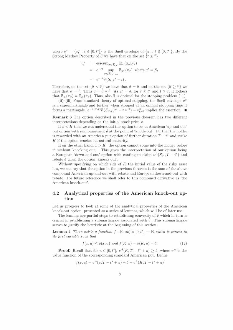
Remark 3 The option described in the previous theorem has two differentinterpretations depending on the initial stock price x.

If x < K then we can understand this option to be an American ‘up-and-out’put option with reimbursement δ at the point of ‘knock-out’. Further the holderis rewarded with an American put option of further duration T − t∗ and strikeK if the option reaches its natural maturity.

If on the other hand, x > K the option cannot come into the money beforet∗ without knocking out. This gives the interpretation of our option beinga European ‘down-and-out’ option with contingent claim vA(St∗ , T − t∗) andrebate δ when the option ‘knocks out’.

Without specifying on which side of K the initial value of the risky assetlies, we can say that the option in the previous theorem is the sum of the abovecompound American up-and-out with rebate and European down-and-out withrebate. For future reference we shall refer to this combined derivative as ‘theAmerican knock-out’.

4.2 Analytical properties of the American knock-out op-tion

Let us progress to look at some of the analytical properties of the Americanknock-out option, presented as a series of lemmas, which will be of later use.

The lemmas are partial steps to establishing convexity of v which in turn iscrucial in establishing a submartingale associated with v. This submartingaleserves to justify the heuristic at the beginning of this section.

Lemma 4 There exists a function f : (0,∞) × [0, t∗] → R which is convex inits first variable such that

f(x, u) ≤ v(x, u) and f(K, u) = v(K, u) = δ. (12)

Proof. Recall that for u ∈ [0, t∗], vA(K, T − t∗ + u) ≥ δ, where vA is thevalue function of the corresponding standard American put. Define

f(x, u) = vA(x, T − t∗ + u) + δ − vA(K, T − t∗ + u)

8

We have of course that f(K, u) = v(K, u) and convexity follows from the factthat vA is known to be convex. It remains to show that

f(x, u) ≤ v(x, u). (13)

As the rebate δ is always smaller than the value of the American put at the strikewe have that v ≤ vA(·, T − t∗ + ·). Thus (13) states that the maximal distancebetween v(x, u) and vA(x, u) is attained at x = K. This seems to be plausibleas the payoffs of the underlying options only differ when St hits K. But, if theprocess St starts away from K it hits K only with some probability and aftersome time. By this, the strong Markov property and the fact that vA(K, ·)is increasing, one can verify (13). For a formal proof write σA as short handfor σA

T−t∗+u, the optimal exercising time for an American put with maturityT − t∗ + u, and recall that τ is the first hitting time of K. We have

v(x, u)

≥ Ex

(e−r(σA∧bτ∧u)v(SσA∧bτ∧u, u − σA ∧ τ ∧ u)

)≥ Exe−r(σA∧bτ∧u)

(1(bτ<σA∧u)δ + 1(bτ≥σA∧u)v

A(SσA∧u, T − t∗ + u − σA ∧ u))

= Ex

(e−r(σA∧bτ∧u)vA(SσA∧bτ∧u, T − t∗ + u − σA ∧ τ ∧ u)

)−Ex

(e−rbτ1(bτ<σA∧u)

(vA(K, T − t∗ + u − τ ) − δ

))≥ Ex

(e−r(σA∧bτ∧u)vA(SσA∧bτ∧u, T − t∗ + u − σA ∧ τ ∧ u)

)−Ex

(1(bτ<σA∧u)

(vA(K, T − t∗ + u) − δ

))≥ Ex

(e−r(σA∧bτ∧u)vA(SσA∧bτ∧u, T − t∗ + u − σA ∧ τ ∧ u)

)−

(vA(K, T − t∗ + u) − δ

)= vA(x, T − t∗ + u) + δ − vA(K, T − t∗ + u)= f(x, u).

The first inequality is due to the supermartingale property stated in Theorem 2.The second inequality can be seen by a case differentiation. In case of τ < σA∧uit is obvious thereas for σA ∧u ≤ τ we use that v(SσA , u−σA) ≥ (K −SσA)+ =vA(SσA , T − t∗ + u − σA) and v(Su, 0) = vA(Su, T − t∗), resp. Then, the firstequality is just rewriting and the third and fourth inequality use that the valueof the American put is increasing in the time to maturity and the differencevA(K, T − t∗ + u) − δ is nonnegative. Finally, the second equality comes fromthe martingale property of the American put.

Lemma 5 We have that for all u ≥ 0 and x > 0, v(x, u) > 0 and

(K − x)+ ≤ v (x, u) ≤ (K − x)+ + δ. (14)

Further, for each x > 0 the function v(x, ·) is monotone increasing and con-tinuous and for each u ∈ [0, t∗] the function v(·, u) is monotone decreasing andcontinuous; and hence v is jointly continuous.

9

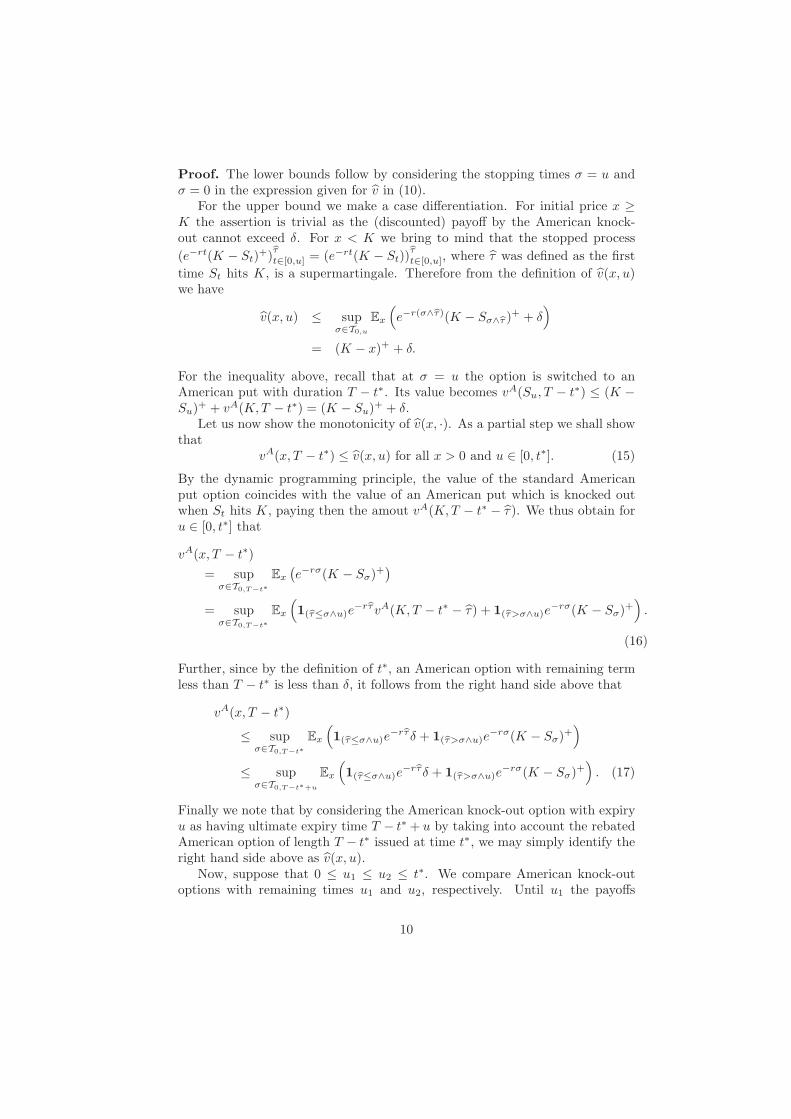
Proof. The lower bounds follow by considering the stopping times σ = u andσ = 0 in the expression given for v in (10).

For the upper bound we make a case differentiation. For initial price x ≥K the assertion is trivial as the (discounted) payoff by the American knock-out cannot exceed δ. For x < K we bring to mind that the stopped process(e−rt(K − St)+)bτ

t∈[0,u] = (e−rt(K − St))bτt∈[0,u], where τ was defined as the first

time St hits K, is a supermartingale. Therefore from the definition of v(x, u)we have

v(x, u) ≤ supσ∈T0,u

Ex

(e−r(σ∧bτ)(K − Sσ∧bτ )+ + δ

)= (K − x)+ + δ.

For the inequality above, recall that at σ = u the option is switched to anAmerican put with duration T − t∗. Its value becomes vA(Su, T − t∗) ≤ (K −Su)+ + vA(K, T − t∗) = (K − Su)+ + δ.

Let us now show the monotonicity of v(x, ·). As a partial step we shall showthat

vA(x, T − t∗) ≤ v(x, u) for all x > 0 and u ∈ [0, t∗]. (15)

By the dynamic programming principle, the value of the standard Americanput option coincides with the value of an American put which is knocked outwhen St hits K, paying then the amout vA(K, T − t∗ − τ ). We thus obtain foru ∈ [0, t∗] that

vA(x, T − t∗)= sup

σ∈T0,T−t∗Ex

(e−rσ(K − Sσ)+

)= sup

σ∈T0,T−t∗Ex

(1(bτ≤σ∧u)e

−rbτvA(K, T − t∗ − τ) + 1(bτ>σ∧u)e−rσ(K − Sσ)+

).

(16)

Further, since by the definition of t∗, an American option with remaining termless than T − t∗ is less than δ, it follows from the right hand side above that

vA(x, T − t∗)

≤ supσ∈T0,T−t∗

Ex

(1(bτ≤σ∧u)e

−rbτδ + 1(bτ>σ∧u)e−rσ(K − Sσ)+

)≤ sup

σ∈T0,T−t∗+u

Ex

(1(bτ≤σ∧u)e

−rbτδ + 1(bτ>σ∧u)e−rσ(K − Sσ)+

). (17)

Finally we note that by considering the American knock-out option with expiryu as having ultimate expiry time T − t∗ + u by taking into account the rebatedAmerican option of length T − t∗ issued at time t∗, we may simply identify theright hand side above as v(x, u).

Now, suppose that 0 ≤ u1 ≤ u2 ≤ t∗. We compare American knock-outoptions with remaining times u1 and u2, respectively. Until u1 the payoffs

10

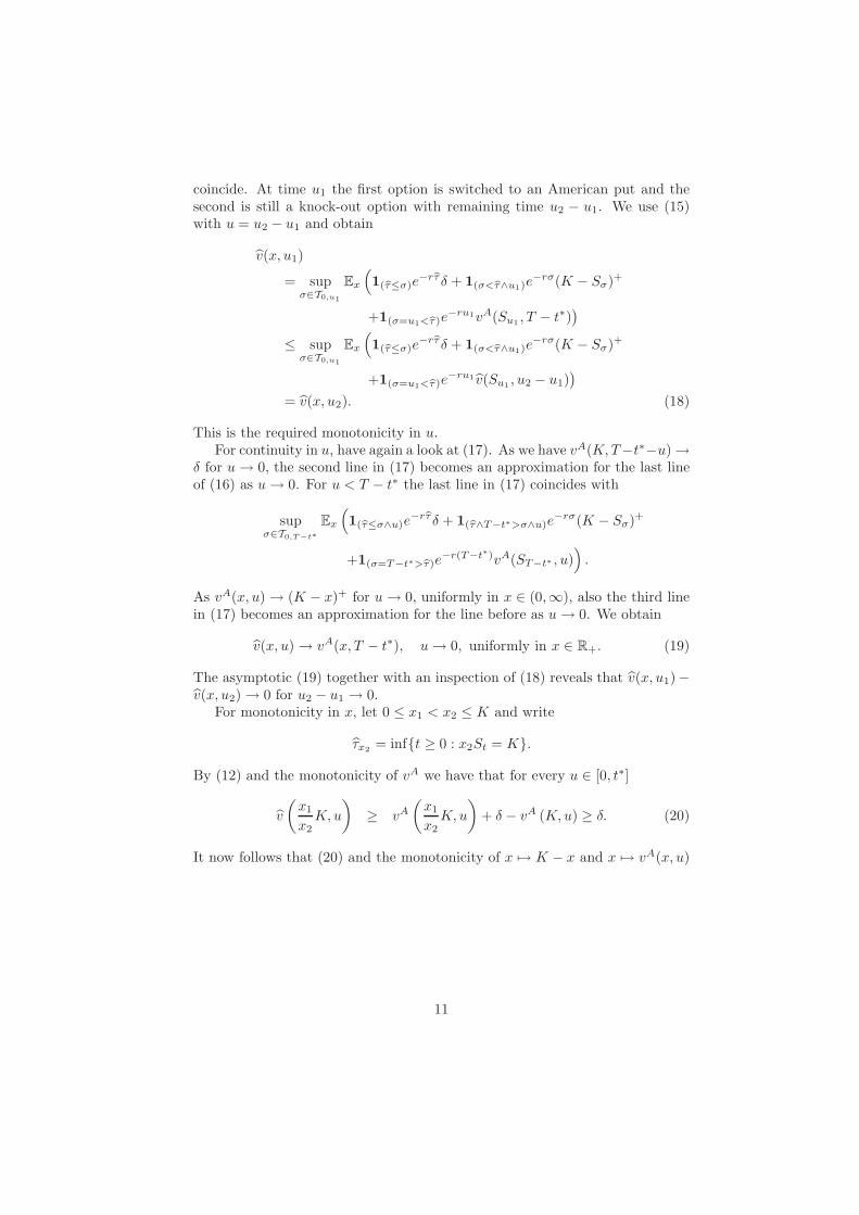
coincide. At time u1 the first option is switched to an American put and thesecond is still a knock-out option with remaining time u2 − u1. We use (15)with u = u2 − u1 and obtain

v(x, u1)

= supσ∈T0,u1

Ex

(1(bτ≤σ)e

−rbτδ + 1(σ<bτ∧u1)e−rσ(K − Sσ)+

+1(σ=u1<bτ)e−ru1vA(Su1 , T − t∗)

)≤ sup

σ∈T0,u1

Ex

(1(bτ≤σ)e

−rbτδ + 1(σ<bτ∧u1)e−rσ(K − Sσ)+

+1(σ=u1<bτ)e−ru1 v(Su1 , u2 − u1)

)= v(x, u2). (18)

This is the required monotonicity in u.For continuity in u, have again a look at (17). As we have vA(K, T−t∗−u) →

δ for u → 0, the second line in (17) becomes an approximation for the last lineof (16) as u → 0. For u < T − t∗ the last line in (17) coincides with

supσ∈T0,T−t∗

Ex

(1(bτ≤σ∧u)e

−rbτδ + 1(bτ∧T−t∗>σ∧u)e−rσ(K − Sσ)+

+1(σ=T−t∗>bτ)e−r(T−t∗)vA(ST−t∗ , u)

).

As vA(x, u) → (K − x)+ for u → 0, uniformly in x ∈ (0,∞), also the third linein (17) becomes an approximation for the line before as u → 0. We obtain

v(x, u) → vA(x, T − t∗), u → 0, uniformly in x ∈ R+. (19)

The asymptotic (19) together with an inspection of (18) reveals that v(x, u1)−v(x, u2) → 0 for u2 − u1 → 0.

For monotonicity in x, let 0 ≤ x1 < x2 ≤ K and write

τx2 = inft ≥ 0 : x2St = K.

By (12) and the monotonicity of vA we have that for every u ∈ [0, t∗]

v

(x1

x2K, u

)≥ vA

(x1

x2K, u

)+ δ − vA (K, u) ≥ δ. (20)

It now follows that (20) and the monotonicity of x → K − x and x → vA(x, u)

11

imply that

v(x2, u)

= supσ∈T0,u

E1

(1(bτx2≤σ)e

−rbτx2δ + 1(σ<bτx2∧u)e−rσ(K − x2Sσ)+

+1(σ=u<bτx2)e−ruvA(x2Su, T − t∗)

)≤ sup

σ∈T0,u

E1

(1(bτx2≤σ)e

−rbτx2 v

(x1

x2K, u − τx2

)+ 1(σ<bτx2∧u)e

−rσ(K − x1Sσ)+

+1(σ=u<bτx2)e−ruvA(x1Su, T − t∗)

)= v(x1, u). (21)

The last equality follows from the dynamic programming principle (Note thatτx2 ≤ inft ≥ 0 : x1St = K). By (14) we have v (Kx1/x2, u) ≤ (K − Kx1/x2)

++δ and therefore

v

(x1

x2K, u

)→ δ, x1 → x2 > 0. (22)

The limiting relation (22) and an inspection of (21) reveals continuity in x.On [K,∞) the proof of monotonicity and continuity is similar, but easier. It

makes again use of the fact that v(x, u) ≥ vA(x, u)+ δ − vA(K, u) → δ, x → K,uniformly in u ∈ [0, t∗]. The complete proof is left to the reader.

The monotonicity properties of v and its lower bounds together with the factthat v(K, u) = δ, this implies that there exists an open set C taking the form

C = (K,∞) × (0, t∗) ∪ (x, u) ∈ (0, K) × (0, t∗) : x > b(u)

where b : (0, t∗] → [0, K), given by

b(u) = supx ≥ 0 : v(x, u) = K − x

(with the convention that sup ∅ = 0) is monotone decreasing, satisfyinglimu↓0 b(u) ≤ ϕA(T − t∗) such that the optimal stopping time τ ∧ σ correspondsto

τC := inft > 0 : (St, t∗ − t) /∈ C

Lemma 6 The value function v(x, u) is twice continuously differentiable in xand once continuously differentiable in u on the continuation region C with

12σ2x2 ∂2v

∂x2+ rx

∂v

∂x− rv − ∂v

∂u= 0 in C.

Proof. We recall a technique used in Karatzas and Shreve (1991), page 243.That is to say, construct the parabolic Dirichlet problem

12σ2x2 ∂2V

∂x2+ rx

∂V

∂x− rV − ∂V

∂u= 0 in R

V = v on ∂0R

12

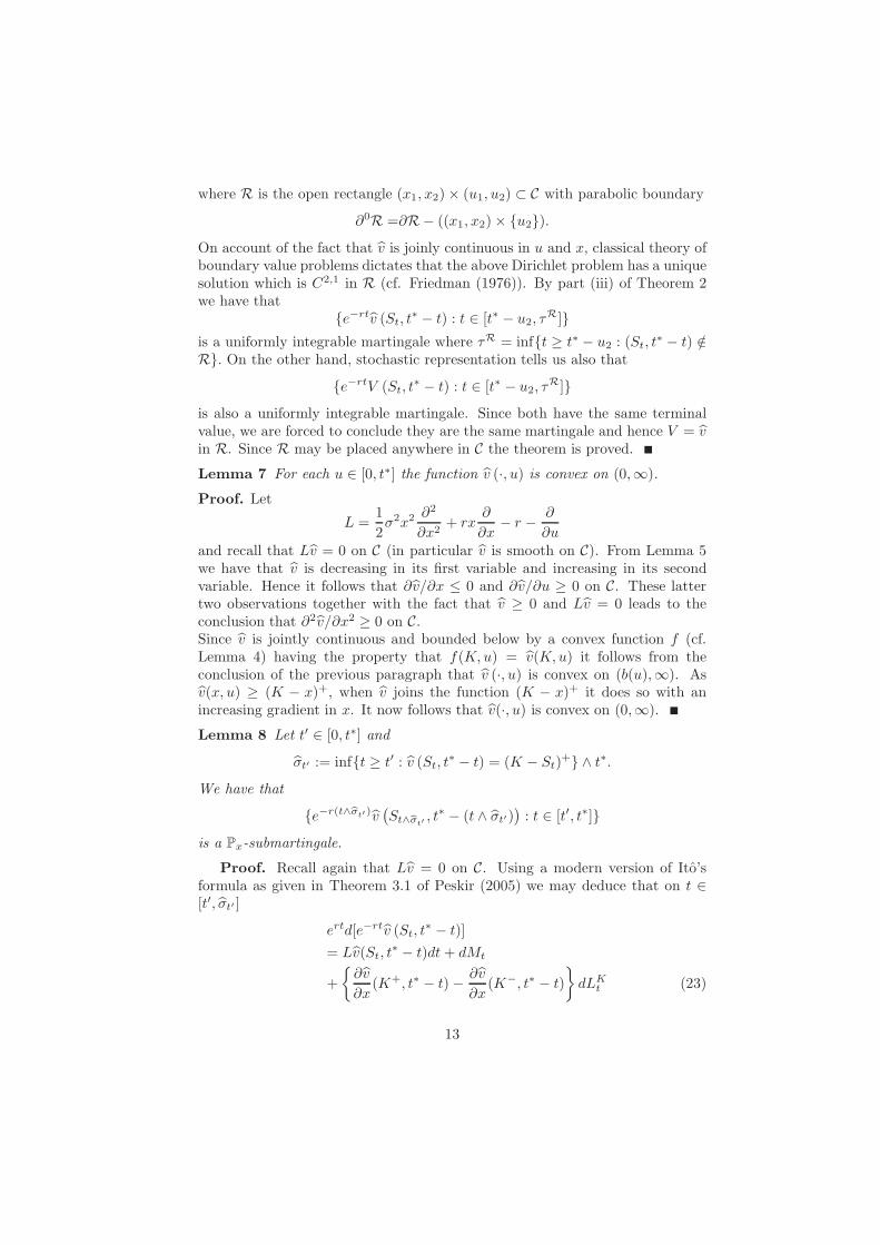
where R is the open rectangle (x1, x2) × (u1, u2) ⊂ C with parabolic boundary

∂0R =∂R− ((x1, x2) × u2).

On account of the fact that v is joinly continuous in u and x, classical theory ofboundary value problems dictates that the above Dirichlet problem has a uniquesolution which is C2,1 in R (cf. Friedman (1976)). By part (iii) of Theorem 2we have that

e−rtv (St, t∗ − t) : t ∈ [t∗ − u2, τ

R]is a uniformly integrable martingale where τR = inft ≥ t∗ − u2 : (St, t

∗ − t) /∈R. On the other hand, stochastic representation tells us also that

e−rtV (St, t∗ − t) : t ∈ [t∗ − u2, τ

R]

is also a uniformly integrable martingale. Since both have the same terminalvalue, we are forced to conclude they are the same martingale and hence V = vin R. Since R may be placed anywhere in C the theorem is proved.

Lemma 7 For each u ∈ [0, t∗] the function v (·, u) is convex on (0,∞).

Proof. Let

L =12σ2x2 ∂2

∂x2+ rx

∂

∂x− r − ∂

∂uand recall that Lv = 0 on C (in particular v is smooth on C). From Lemma 5we have that v is decreasing in its first variable and increasing in its secondvariable. Hence it follows that ∂v/∂x ≤ 0 and ∂v/∂u ≥ 0 on C. These lattertwo observations together with the fact that v ≥ 0 and Lv = 0 leads to theconclusion that ∂2v/∂x2 ≥ 0 on C.Since v is jointly continuous and bounded below by a convex function f (cf.Lemma 4) having the property that f(K, u) = v(K, u) it follows from theconclusion of the previous paragraph that v (·, u) is convex on (b(u),∞). Asv(x, u) ≥ (K − x)+, when v joins the function (K − x)+ it does so with anincreasing gradient in x. It now follows that v(·, u) is convex on (0,∞).

Lemma 8 Let t′ ∈ [0, t∗] and

σt′ := inft ≥ t′ : v (St, t∗ − t) = (K − St)+ ∧ t∗.

We have that

e−r(t∧bσt′)v(St∧bσt′ , t

∗ − (t ∧ σt′))

: t ∈ [t′, t∗]

is a Px-submartingale.

Proof. Recall again that Lv = 0 on C. Using a modern version of Ito’sformula as given in Theorem 3.1 of Peskir (2005) we may deduce that on t ∈[t′, σt′ ]

ertd[e−rtv (St, t∗ − t)]

= Lv(St, t∗ − t)dt + dMt

+

∂v

∂x(K+, t∗ − t) − ∂v

∂x(K−, t∗ − t)

dLK

t (23)

13

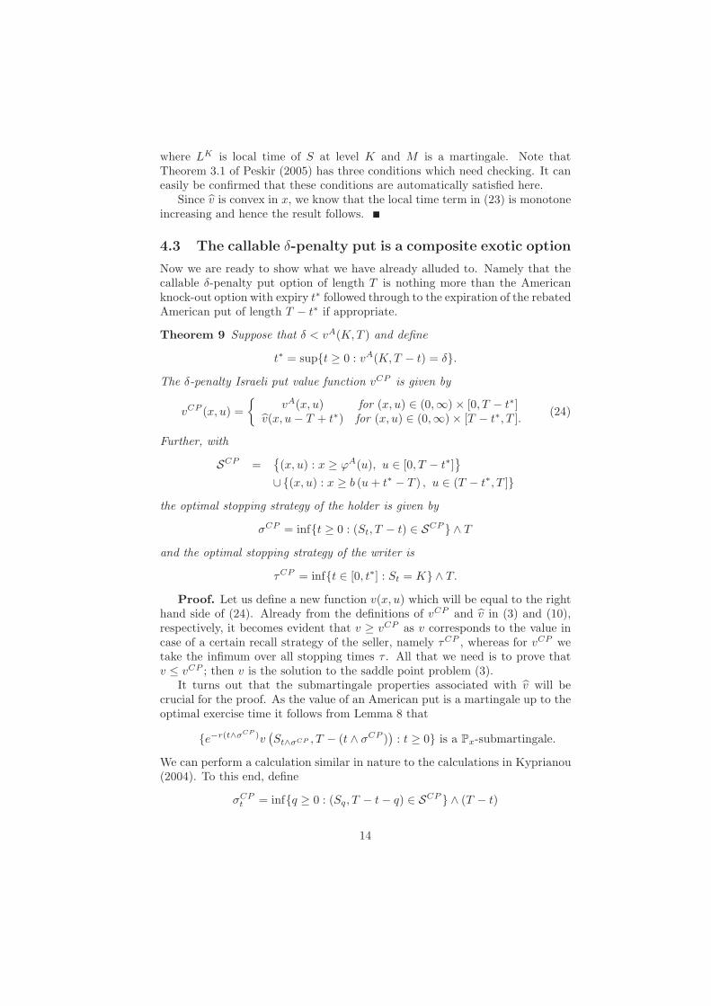
where LK is local time of S at level K and M is a martingale. Note thatTheorem 3.1 of Peskir (2005) has three conditions which need checking. It caneasily be confirmed that these conditions are automatically satisfied here.

Since v is convex in x, we know that the local time term in (23) is monotoneincreasing and hence the result follows.

4.3 The callable δ-penalty put is a composite exotic option

Now we are ready to show what we have already alluded to. Namely that thecallable δ-penalty put option of length T is nothing more than the Americanknock-out option with expiry t∗ followed through to the expiration of the rebatedAmerican put of length T − t∗ if appropriate.

Theorem 9 Suppose that δ < vA(K, T ) and define

t∗ = supt ≥ 0 : vA(K, T − t) = δ.

The δ-penalty Israeli put value function vCP is given by

vCP (x, u) =

vA(x, u) for (x, u) ∈ (0,∞) × [0, T − t∗]v(x, u − T + t∗) for (x, u) ∈ (0,∞) × [T − t∗, T ]. (24)

Further, with

SCP =(x, u) : x ≥ ϕA(u), u ∈ [0, T − t∗]

∪(x, u) : x ≥ b (u + t∗ − T ) , u ∈ (T − t∗, T ]

the optimal stopping strategy of the holder is given by

σCP = inft ≥ 0 : (St, T − t) ∈ SCP ∧ T

and the optimal stopping strategy of the writer is

τCP = inft ∈ [0, t∗] : St = K ∧ T.

Proof. Let us define a new function v(x, u) which will be equal to the righthand side of (24). Already from the definitions of vCP and v in (3) and (10),respectively, it becomes evident that v ≥ vCP as v corresponds to the value incase of a certain recall strategy of the seller, namely τCP , whereas for vCP wetake the infimum over all stopping times τ . All that we need is to prove thatv ≤ vCP ; then v is the solution to the saddle point problem (3).

It turns out that the submartingale properties associated with v will becrucial for the proof. As the value of an American put is a martingale up to theoptimal exercise time it follows from Lemma 8 that

e−r(t∧σCP )v(St∧σCP , T − (t ∧ σCP )

): t ≥ 0 is a Px-submartingale.

We can perform a calculation similar in nature to the calculations in Kyprianou(2004). To this end, define

σCPt = infq ≥ 0 : (Sq, T − t − q) ∈ SCP ∧ (T − t)

14

and

τCPt =

infq ∈ [0, t∗ − t] : Sq = K ∧ (T − t) if t ≤ t∗

T − t if t > t∗.

That is when x′ = St

v (x′, T − t)

= infτ∈T0,T−t

Ex′(e−r(τ∧σCP

t )v(Sτ∧σCP

t, T − t − (τ ∧ σCP

t )))

≤ infτ∈T0,T−t

Ex′(e−r(τ∧σCP

t )1(σCP

t ≤τ)(K − SσCPt

)+ + 1(σCPt >τ)[(K − Sτ )+ + δ]

)≤ sup

σ∈T0,T−t

infτ∈T0,T−t

Ex′(e−r(τ∧σ)

1(σ≤τ)(K − Sσ)+ + 1(σ>τ)[(K − Sτ )+ + δ]

)= vCP (x′, T − t)

where the first equality holds by Lemma 8 and the corresponding martingaleproperty for the American put. In the first inequality we have used thatv

(SσCP

t, T − t − σCP

)= (K − SσCP

t)+ and the fact that (K − x)+ + δ is an

upper bound for v. The latter follows from (14) and the estimation vA(x, u) ≤(K − x)+ + vA(K, u) ≤ (K − x)+ + δ for American puts with duration u lessthan T − t∗.

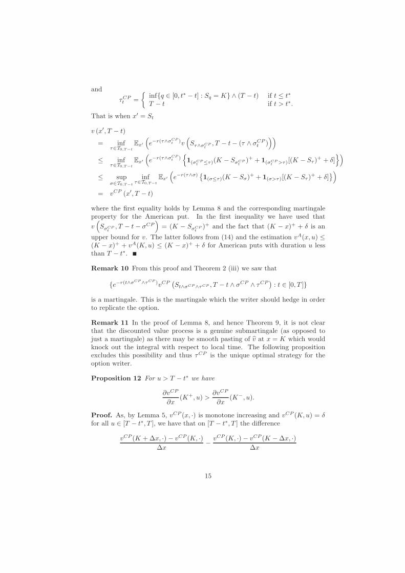
Remark 10 From this proof and Theorem 2 (iii) we saw that

e−r(t∧σCP∧τCP )vCP(St∧σCP ∧τCP , T − t ∧ σCP ∧ τCP

): t ∈ [0, T ]

is a martingale. This is the martingale which the writer should hedge in orderto replicate the option.

Remark 11 In the proof of Lemma 8, and hence Theorem 9, it is not clearthat the discounted value process is a genuine submartingale (as opposed tojust a martingale) as there may be smooth pasting of v at x = K which wouldknock out the integral with respect to local time. The following propositionexcludes this possibility and thus τCP is the unique optimal strategy for theoption writer.

Proposition 12 For u > T − t∗ we have

∂vCP

∂x(K+, u) >

∂vCP

∂x(K−, u).

Proof. As, by Lemma 5, vCP (x, ·) is monotone increasing and vCP (K, u) = δfor all u ∈ [T − t∗, T ], we have that on [T − t∗, T ] the difference

vCP (K + ∆x, ·) − vCP (K, ·)∆x

− vCP (K, ·) − vCP (K − ∆x, ·)∆x

15

is monotone increasing for all ∆x > 0 and therewith also its limit

∂vCP

∂x(K+, ·) − ∂vCP

∂x(K−, ·) (25)

(letting ∆x tend to zero). By convexity the difference in (25) is nonnegative.Assume that it vanishes for a fixed u ∈ (T − t∗, T ]. Then, it has to vanishfor all u′ ∈ (T − t∗, u] and the local time part in (23) disappears after T − u.Consequently, the process t → e−rtvCP (St, T − t) started at t = T − u is asupermartingale which impies that vCP (·, u) = vA(·, u) (as the price processof the American put is the smallest supermartingale dominating the intrinsicoption value). This contradicts to vCP (K, u) = δ = vA(K, T − t∗) < vA(K, u)for u ∈ (T − t∗, T ].

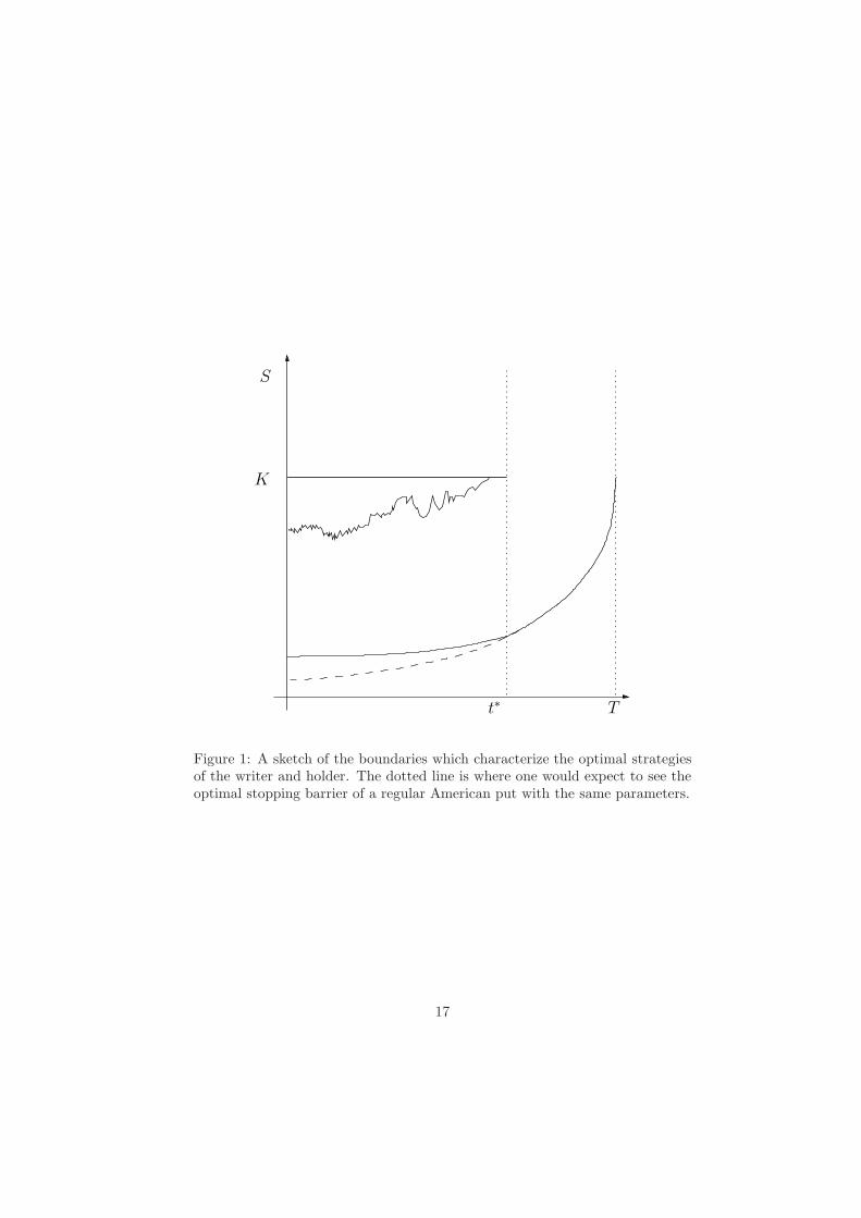
Let us conclude this section with some sketches of aspects of the functionvCP . Figure 1 gives an impression of the two barriers which form the saddlepoint strategy of the stochastic game behind the callable put. The upper barrierat S = K represents the stopping region of the writer and the domain belowthe lower curved line represents the stopping domain of the writer. The dottedline represents the continuation of the barrier in the case of a regular Americanput with the same parameters.

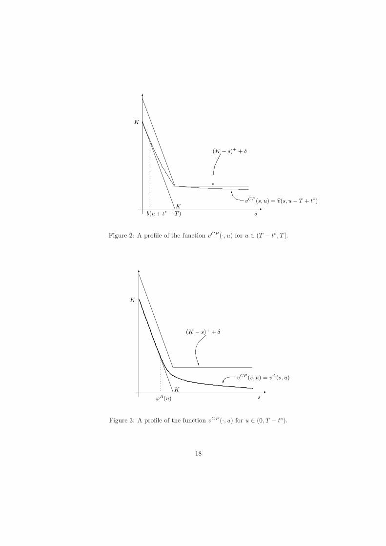
In Figures 2 and 3 depict time slices of the function vCP (x, u). Figure 2 isa time slice from the region where T ≥ u > T − t∗. The profile of vCP (·, u) isconstrained by the upper and lower gain functions (K − x)+ + δ and (K − x)+

respectively. Further, the value function pastes smoothly onto the lower gainfunction and fits under the corner of the upper gain function with a discontinuityin its first derivative as indicated in the previous proposition.

In Figure 3 we see vCP (·, u) closer to the expiry of the option when 0 <u < T − t∗. In this case, the callable put has the same value as an Americanput with the same parameters close to expiry. One sees in the figure that theupper gain function is everywhere strictly greater than the value curve whichis consistent with the logic that the writer of the callable put prefers never toexercise close to expiry.

5 Conclusion

We have shown that the callable put is equivalent to the composition of otherknown exotic options. That is to say the stochastic saddle point in Kifer’spricing formula of game contingent claims is semi-explicitly identifiable thusgiving a basis for further research of these options. Indeed with further work,one should be able to show that the given composite exotic options characterizeuniquely the solution to a free boundary problem as one sees for Americanput and Russian options. See the preprint preceding this article, Kuhn andKyprianou (2003a).

In related work, the reader is also referred to Kuhn and Kyprianou (2003b)where the value of a more general class of finite expiry game contingent claimsare characterized via a pathwise pricing formula.

16

S

K

t∗ T

Figure 1: A sketch of the boundaries which characterize the optimal strategiesof the writer and holder. The dotted line is where one would expect to see theoptimal stopping barrier of a regular American put with the same parameters.

17

(K − s)+ + δ

vCP (s, u) = bv(s, u − T + t∗)

b(u + t∗ − T )

K

sK

Figure 2: A profile of the function vCP (·, u) for u ∈ (T − t∗, T ].

(K − s)+ + δ

ϕA(u)

vCP (s, u) = vA(s, u)

K

s

K

Figure 3: A profile of the function vCP (·, u) for u ∈ (0, T − t∗).

18

References

[1] Allen, L. and Saunders, A. (1993) Forbearance and valuation of depositinsurance as a callable put. Journal of Banking and Finance 17, 629–643.

[2] Duistermaat, J.J., Kyprianou, A.E. and van Schaik, K. (2005) Finite expiryRussian options. Stoch. Proc. Appl. 115, 609–638.

[3] Friedman, A. (1976) Stochastic differential equations and applications. VolI. Academic Press.

[4] Karatzas, I. and Shreve, S. (1991) Brownian Motion and Stochastic Calculus.Springer.

[5] Karatzas, I. and Shreve, S. (1998) Methods of Mathematical Finance.Springer.

[6] Kifer, Y. (2000) Game options. Finance & Stochastics 4, 443–463.

[7] Kuhn, C. and Kyprianou, A.E. (2003a) Israeli options as composite exoticoptions. Preprint, University of Utrecht.

[8] Kuhn, C. and Kyprianou, A.E. (2003b) Pricing Israeli options: a pathwiseapproach. Preprint, University of Utrecht.

[9] Kyprianou, A.E. (2004) Some calculations for Israeli options. Finance &Stochastics 8, 73 - 86.

[10] Lamberton, D. (1998) American Options. In Statistics of Finance eds D.Hand and S. D. Jacka. Arnold.

[11] Myneni, R. (1992) The pricing of the American option. Ann. Appl. Probab.2, no. 1, 1–23.

[12] Peskir, G. (2005) A change-of-variable formula with local time on curves.Journal of Theoretical Probability 18, 499–535.

[13] Shepp, L.A. and Shiryaev, A.N. (1993) The Russian option: reduced regret.Ann. Appl. Probab. 3, 603–631.

[14] Shepp, L.A. and Shiryaev, A.N. (1995) A new look at pricing of the “Rus-sian option”. Theory Probab. Appl. 39, 103–119.

[15] Shiryaev, A. N., Kabanov, Yu. M., Kramkov, D. O. and Melc’nikov, A.V. (1995) Towards a theory of pricing options of European and Americantypes. II. Continuous time. (Russian) Translation in Theory Probab. Appl.39 61–102.

19