camels ccdas a bayesian approach and metropolis monte carlo method to estimate parameters and...
TRANSCRIPT

CAMELSCCDAS
A Bayesian approach and Metropolis Monte Carlo method
to estimate parameters and uncertainties
in ecosystem models from eddy-covariance data
CAMELS Meeting, Wageningen, 11.- 12. November 2003
Jens KattgeWolfgang Knorr

CAMELSCCDAS
Outlines
• Methodo Bayesian approach o Metropolis algorithm
• Model: BETHY
• Eddy covariance data: Loobos site
• Resultso Sampling parameter setso Selecting parameter sets representing the a posteriori PDFo Using the selected parameter sets
– Calculate first moments of the PDF in parameter space– Propagate parameter uncertainties into modeled fluxes
• Conclusions and Perspectives
CAMELSCCDAS
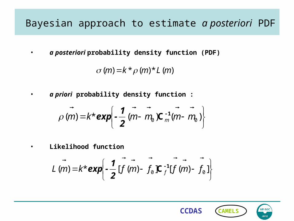
Bayesian approach to estimate a posteriori PDF
• a posteriori probability density function (PDF)
• a priori probability density function :
• Likelihood function
)(*)(*)( mLmkm
)()(*)( 00 mmmmkm m
-1C2
1-exp
])([])([*)( 00 fmffmfkmL f
-1C2
1-exp

CAMELSCCDAS
Metropolis algorithm to sample a posteriori PDF
• Metropolis algorithm: • Markov Chain Monte Carlo (MCMC) methods: Metropolis, Metropolis-
Hastings, Gibbs Sampler ….
• Guided random walks:
after walking from the starting point towards the maximum of the PDF (burn-in time), the walker samples the target distribution: probability in PDF >>> frequency in sampling
• Metropolis decision:
if accept step
if accept step with probability
1)(/)( ppp i
)(/)( ppp i1)(/)( ppp i

CAMELSCCDAS
Model: BETHY parameters and uncertainties
Parameter
Description
vcmax maximum carboxylation ratejmvm relationship of jmax and vcmax aq quantum efficiencykc Michaelis-Menten constant for CO2 at 25 °Cko Michaelis-Menten constant for O2 at 25 °Cec activation energy for kceo activation energy for koev activation energy for vcmaxgam proportionality of CO2 compensation point and canopy temperature frd relationship of. dark resp and vm er activation energy for dark respirationfrl ratio of leaf to total maintenance respiration fci non water limited relationship of ci and ca cw maximum water supply rate of root systemav albedo of vegetation surface for vegetation cover asoil solar radiation absorbed by soil under vegetation ep sky emissivity factor ω single scattering albedo of leaves fc fraction of vegetation cover fga vegetation factor of atmospheric conductance rsoil soil respiration at 10 °C and field capacity q10 Q10 of soil respiration kw soil water factor of soil respiration swc soil water content at pF 4.2 (permanent wilting point)
Assumed uncertainty of parameters: SD = 0.1, 0.25, 0.5

CAMELSCCDAS
Eddy Covariance Data: Loobos site
• Halfhourly data of Eddy covariance measurements from seven days during 1997 and 1998 from the Loobos site in the Netherlands
• PFT: coniferous forest
• Diagnostics: NEE and LH
NEE LH

CAMELSCCDAS
Random walk in parameter space
After transition from the starting point to the region of highest probability, the walker samples the target distribution.

CAMELSCCDAS
Convergence of average values

CAMELSCCDAS
Does the algorithm find the global optimum?
It depends on the starting point.

CAMELSCCDAS
Does the algorithm find the global optimum?
Sequences from different points lead to different “optima”.

CAMELSCCDAS
Gelman’s empirical decision of convergence
W
Bn
Wn
n
R
11
n: number of sequencesW: average of variancesB: variance of averages
Empirical reduction factor R (Gelman et al., 1992) :Sequences have converged to a common target distribution, if the average of variances within sequences dominates the variance of averages between sequences:

CAMELSCCDAS
Using the sampling: parameter means and SD
a priori SD:
0.1
0.25
0.5

CAMELSCCDAS
Using the sampling: relative reduction of error
a priori SD:
0.1
0.25
0.5

CAMELSCCDAS
Using the sampling: parameter correlations
vm jmvm aq kc ko ec eo ev gam frd er frl fci cw av asoil ep o fc fga rsoil q10 kw swc1 -0.64 0.07 0.31 -0.1 -0.27 0.07 0.41 0.34 -0.21 0.09 0.05 -0.02 0.21 -0.06 0.07 -0.04 -0.05 0.17 0.1 -0.01 0.1 0.16 0.2 vm
1 0.11 -0.42 0.11 0.18 0 -0.16 0.05 0.1 -0.05 -0.04 -0.07 -0.06 0.08 -0.07 0.17 0 -0.23 0.07 0.05 -0.04 -0.08 -0.09 jmvm1 0.05 -0.01 0.18 -0.07 -0.14 0.15 0.08 -0.07 -0.08 0.19 -0.29 -0.01 0.01 0.2 0.03 -0.71 -0.1 -0.02 -0.13 0 -0.03 aq
1 0.17 0.33 -0.12 -0.31 -0.34 -0.05 -0.03 0.03 0.16 -0.09 0.07 0.11 0.06 0.02 -0.29 0.02 -0.03 -0.2 -0.01 -0.02 kc1 -0.11 0.04 0.1 0.05 -0.02 0 -0.04 -0.06 0.02 0.01 -0.03 0.01 0.06 0.05 0.01 0.01 0.03 -0.01 0 ko
1 -0.04 -0.17 -0.28 0.07 -0.08 -0.04 0.19 -0.18 0.11 0.04 0.11 -0.01 -0.37 0.09 0.04 -0.19 -0.06 -0.05 ec1 0.11 0.12 -0.02 0.06 0.05 -0.09 0.09 -0.02 -0.03 0 -0.05 0.14 0.01 0.03 0.04 0 0.04 eo
1 0.44 -0.15 0.07 0 -0.06 0.21 -0.07 -0.02 -0.15 -0.02 0.42 -0.01 0.04 0.17 0.11 0.17 ev1 -0.04 -0.03 -0.03 0 0.22 -0.01 -0.01 -0.17 -0.01 0.34 0.08 0.01 0.02 0.15 0.2 gam
1 0.08 0.17 0.13 -0.02 0.02 -0.06 -0.04 0.02 -0.04 0 -0.04 -0.11 0.21 0.02 frd1 0.03 -0.05 0.02 0.01 0 -0.04 0 0.07 0.08 0.13 -0.08 -0.2 -0.02 er
1 -0.09 0.09 -0.04 0 0.13 0.03 0 0.01 0.12 0.12 -0.25 0 frl1 -0.32 0.18 0.06 -0.34 0.01 -0.2 -0.22 -0.11 -0.17 0.01 0.15 fci
1 -0.17 -0.04 0.17 -0.05 0.27 0.14 0.04 0.23 0.16 0.68 cw1 0 -0.08 0.01 -0.03 -0.24 -0.04 -0.01 -0.01 -0.06 av
1 -0.01 0 -0.02 -0.04 0.02 -0.01 0.02 0 asoil1 -0.02 -0.49 0.4 0.03 -0.03 0.03 0.1 ep
1 0 -0.08 -0.01 -0.01 -0.04 -0.05 o1 0.07 0.02 0.2 0.05 0.08 fci
1 0.03 0.02 0.01 0.11 fga1 -0.29 0.17 0 rsoil
1 0.38 0.12 q101 0.16 kw
1 swc
corr(vm,jmvm) = -0.64 >> ac = min(f(vm,jmvm))corr(cw,swc) = 0.68 >> root water supply = f(cw,1/swc)

CAMELSCCDAS
Does the a posteriori PDF include non Gaussian components?
Projection of the multi-dimensional PDFonto the dimension of single parameters.
vm cw

CAMELSCCDAS
Modeled fluxes
Fluxes with mean parameters are somehow closer to the obsevations.
CAMELSCCDAS
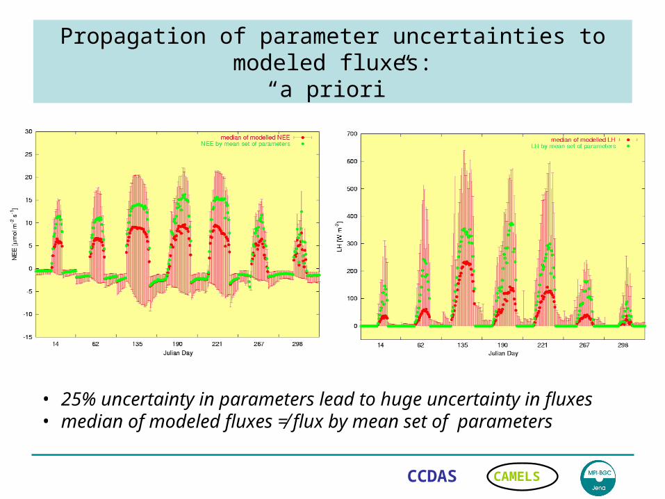
Propagation of parameter uncertainties to modeled fluxes:“a priori”
• 25% uncertainty in parameters lead to huge uncertainty in fluxes • median of modeled fluxes ≠ flux by mean set of parameters

CAMELSCCDAS
Propagation of parameter uncertainties to modeled fluxes
NEE

CAMELSCCDAS
Propagation of parameter uncertainties to modeled fluxes
LH

CAMELSCCDAS
Propagation of parameter uncertainties to modeled fluxes
GPP
CAMELSCCDAS
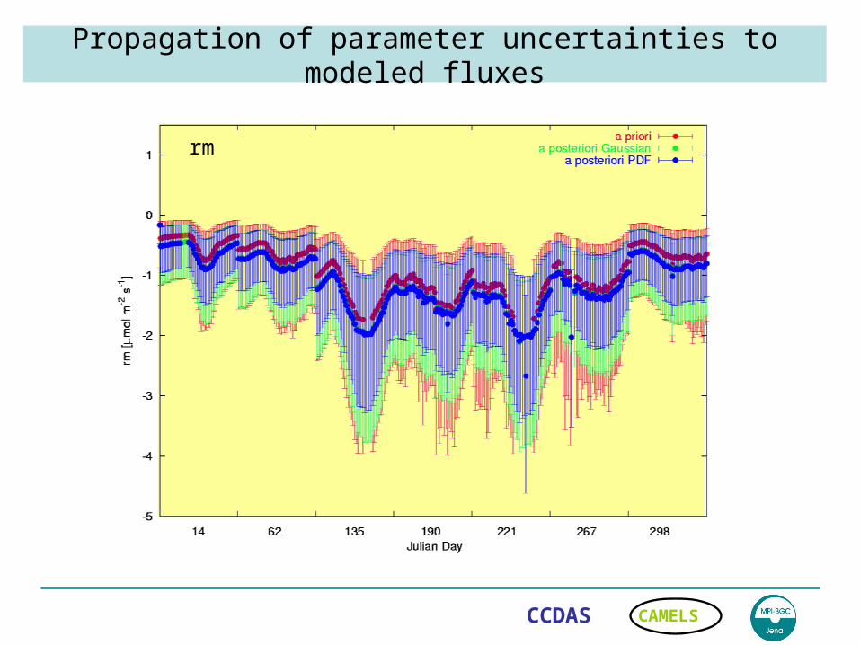
Propagation of parameter uncertainties to modeled fluxes
rm

CAMELSCCDAS
Propagation of parameter uncertainties to modeled fluxes
RH

CAMELSCCDAS
Propagation of parameter uncertainties to modeled fluxes
GC

CAMELSCCDAS
Conclusions
• The Method seems capable of sampling points in parameter space representing the region of the global maximum of the a posteriori PDF.
• The sampling can be used to derive means, errors and covariances (1st&2nd moments of PDF).
• The PDF has non-Gaussian components.
• Some Parameters are constrained by a posteriori PDF.
• Using the complete a posteriori PDF could strongly reduce uncertainties in prognostics.
• Results depend on a priori parameter values and uncertainties and on number and uncertainty of measurements (Bayesian approach).

CAMELSCCDAS
Status quo and Perspectives for MC simulations
Reduce uncertainties in a priori parameter values of global simulations = CAMELS approach to spatial extrapolation of flux measurements
• Status quo:• Routines for data preparation finished, more than 20 sites available (Isabel).• Routines for parameter “optimisation” finished and tested.
• Next steps: • Reduce uncertainties in a priori parameter values (12.2003).
• Get good information of measurement errors (12.2003).
• Get a measure of the sampling error involved in parameter generalisation:• within sites (03.2004),• between sites of the same Plant Functional Type (05.2004).
• Perspectives:• Estimate optimised parameters, uncertainties and covariances for all PFT’s,
based on more than one measurement site per PFT as a priori parameter sets in WP4 (11.2004).
• Comparison between TEM and inventory based approaches (11.2004).