HAL Id: inria-00590269https://hal.inria.fr/inria-00590269

Submitted on 3 May 2011

HAL is a multi-disciplinary open accessarchive for the deposit and dissemination of sci-entific research documents, whether they are pub-lished or not. The documents may come fromteaching and research institutions in France orabroad, or from public or private research centers.

L’archive ouverte pluridisciplinaire HAL, estdestinée au dépôt et à la diffusion de documentsscientifiques de niveau recherche, publiés ou non,émanant des établissements d’enseignement et derecherche français ou étrangers, des laboratoirespublics ou privés.

Camera Models and Fundamental Concepts Used inGeometric Computer Vision

Peter Sturm, Srikumar Ramalingam, Jean-Philippe Tardif, Simone Gasparini,Joao Barreto

To cite this version:Peter Sturm, Srikumar Ramalingam, Jean-Philippe Tardif, Simone Gasparini, Joao Barreto. CameraModels and Fundamental Concepts Used in Geometric Computer Vision. Foundations and Trendsin Computer Graphics and Vision, Now Publishers, 2011, 6 (1-2), pp.1-183. �10.1561/0600000023�.�inria-00590269�

Foundations and TrendsR© inComputer Graphics and VisionVol. 6, Nos. 1–2 (2010) 1–183c© 2011 P. Sturm, S. Ramalingam, J.-P. Tardif,S. Gasparini and J. BarretoDOI: 10.1561/0600000023

Camera Models and Fundamental ConceptsUsed in Geometric Computer Vision

By Peter Sturm, Srikumar Ramalingam,Jean-Philippe Tardif, Simone Gasparini

and Joao Barreto

Contents

1 Introduction and Background Material 3

1.1 Introduction 31.2 Background Material 6

2 Technologies 8

2.1 Moving Cameras or Optical Elements 82.2 Fisheyes 142.3 Catadioptric Systems 152.4 Stereo and Multi-camera Systems 312.5 Others 33

3 Camera Models 36

3.1 Global Camera Models 413.2 Local Camera Models 663.3 Discrete Camera Models 723.4 Models for the Distribution of Camera Rays 753.5 Overview of Some Models 823.6 So Many Models . . . 84

4 Epipolar and Multi-view Geometry 90

4.1 The Calibrated Case 914.2 The Uncalibrated Case 924.3 Images of Lines and the Link between Plumb-line

Calibration and Self-calibration of Non-perspectiveCameras 100

5 Calibration Approaches 103

5.1 Calibration Using Calibration Grids 1035.2 Using Images of Individual Geometric Primitives 1105.3 Self-calibration 1145.4 Special Approaches Dedicated to Catadioptric Systems 124

6 Structure-from-Motion 127

6.1 Pose Estimation 1286.2 Motion Estimation 1306.3 Triangulation 1336.4 Bundle Adjustment 1346.5 Three-Dimensional Scene Modeling 1366.6 Distortion Correction and Rectification 137

7 Concluding Remarks 143

Acknowledgements 145

References 146

Foundations and TrendsR© inComputer Graphics and VisionVol. 6, Nos. 1–2 (2010) 1–183c© 2011 P. Sturm, S. Ramalingam, J.-P. Tardif,S. Gasparini and J. BarretoDOI: 10.1561/0600000023

Camera Models and Fundamental ConceptsUsed in Geometric Computer Vision

Peter Sturm1, Srikumar Ramalingam2,Jean-Philippe Tardif3, Simone Gasparini4,

and Joao Barreto5

1 INRIA Grenoble — Rhone-Alpes and Laboratoire Jean Kuntzmann,Grenoble, Montbonnot, France, Peter.Sturm@inrialpes.fr

2 MERL, Cambridge, MA, USA, ramalingam@merl.com3 NREC — Carnegie Mellon University, Pittsburgh, PA, USA,

tardifj@gmail.com4 INRIA Grenoble — Rhone-Alpes and Laboratoire Jean Kuntzmann,

Grenoble, Montbonnot, France, Simone.Gasparini@inrialpes.fr5 Coimbra University, Coimbra, Portugal, jpbar@deec.uc.pt

Abstract

This survey is mainly motivated by the increased availability and useof panoramic image acquisition devices, in computer vision and variousof its applications. Different technologies and different computationalmodels thereof exist and algorithms and theoretical studies for geomet-ric computer vision (“structure-from-motion”) are often re-developedwithout highlighting common underlying principles. One of the goalsof this survey is to give an overview of image acquisition methodsused in computer vision and especially, of the vast number of cam-era models that have been proposed and investigated over the years,

where we try to point out similarities between different models. Resultson epipolar and multi-view geometry for different camera models arereviewed as well as various calibration and self-calibration approaches,with an emphasis on non-perspective cameras. We finally describe whatwe consider are fundamental building blocks for geometric computervision or structure-from-motion: epipolar geometry, pose and motionestimation, 3D scene modeling, and bundle adjustment. The main goalhere is to highlight the main principles of these, which are independentof specific camera models.

1Introduction and Background Material

1.1 Introduction

Many different image acquisition technologies have been investigatedin computer vision and other areas, many of them aiming at providinga wide field of view. The main technologies consist of catadioptric andfisheye cameras as well as acquisition systems with moving parts, e.g.,moving cameras or optical elements. In this monograph, we try to givean overview of the vast literature on these technologies and on com-putational models for cameras. Whenever possible, we try to point outlinks between different models. Simply put, a computational model fora camera, at least for its geometric part, tells how to project 3D entities(points, lines, etc.) onto the image, and vice versa, how to back-projectfrom the image to 3D. Camera models may be classified according todifferent criteria, for example the assumption or not of a single view-point or their algebraic nature and complexity. Also, recently severalapproaches for calibrating and using “non-parametric” camera mod-els have been proposed by various researchers, as opposed to classical,parametric models.

In this survey, we propose a different nomenclature as our maincriterion for grouping camera models. The main reason is that even

3

4 Introduction and Background Material

so-called non-parametrics models do have parameters, e.g., the coor-dinates of camera rays. We thus prefer to speak of three categories:(i) A global camera model is defined by a set of parameters suchthat changing the value of any parameter affects the projection func-tion all across the field of view. This is the case for example withthe classical pinhole model and with most models proposed for fish-eye or catadioptric cameras. (ii) A local camera model is defined bya set of parameters, each of which influences the projection functiononly over a subset of the field of view. A hypothetical example, justfor illustration, would be a model that is “piecewise-pinhole”, definedover a tessellation of the image area or the field of view. Other exam-ples are described in this monograph. (iii) A discrete camera modelhas sets of parameters for individual image points or pixels. To workwith such a model, one usually needs some interpolation scheme sincesuch parameter sets can only be considered for finitely many imagepoints. Strictly speaking, discrete models plus an interpolation schemeare thus not different from the above local camera models, since modelparameters effectively influence the projection function over regions asopposed to individual points. We nevertheless preserve the distinctionbetween discrete and local models, since in the case of discrete models,the considered regions are extremely small and since the underlyingphilosophies are somewhat different for the two classes of models.

These three types of models are illustrated in Figure 1.1, where thecamera is shown as a black box. As discussed in more detail later inthe monograph, we mainly use back-projection to model cameras, i.e.,the mapping from image points to camera rays. Figure 1.1 illustratesback-projection for global, discrete and local camera models.

After describing camera models, we review central concepts of geo-metric computer vision, including camera calibration, epipolar andmulti-view geometry, and structure-from-motion tasks, such as poseand motion estimation. These concepts are exhaustively described forperspective cameras in recent textbooks [137, 213, 328, 336, 513]; ouremphasis will thus be on non-perspective cameras. We try to describethe various different approaches that have been developed for cameracalibration, including calibration using grids or from images of higherlevel primitives, like lines and spheres, and self-calibration. Throughout

1.1 Introduction 5

Fig. 1.1 Types of camera models. Left : For global models, the camera ray associated withan image point q is determined by the position of q and a set of global camera parameterscontained in a vector c. Middle: For discrete models, different image regions are endowedwith different parameter sets. Right : For discrete models, the camera rays are directly givenfor sampled image points, e.g., by a look-up table containing Plucker coordinates, here thePlucker coordinates Lq of the ray associated with image point q.

this monograph, we aim at describing concepts and ideas rather thanall details, which may be found in the original references.

The monograph is structured as follows. In the following section,we give some background material that aims at making the math-ematical treatment presented in this monograph, self-contained. InSection 2, we review image acquisition technologies, with an emphasison omnidirectional systems. Section 3 gives a survey of computationalcamera models in the computer vision and photogrammetry literature,again emphasizing omnidirectional cameras. Results on epipolar andmulti-view geometry for non-perspective cameras are summarized

6 Introduction and Background Material

in Section 4. Calibration approaches are explained in Section 5,followed by an overview of some fundamental modules for structure-from-motion in Section 6. The monograph ends with conclusions, inSection 7.

1.2 Background Material

Given the large scope of this monograph, we rather propose summariesof concepts and results than detailed descriptions, which would requirean entire book. This allows us to keep the mathematical level at a min-imum. In the following, we explain the few notations we use in thismonograph. We assume that the reader is familiar with basic notionsof projective geometry, such as homogeneous coordinates, homogra-phies, etc. and of multi-view geometry for perspective cameras, such asthe fundamental and essential matrices and projection matrices. Goodoverviews of these concepts are given in [137, 213, 328, 336, 513].

Fonts. We denote scalars by italics, e.g., s, vectors by bold charac-ters, e.g., t and matrices in sans serif, e.g., A. Unless otherwise stated,we use homogeneous coordinates for points and other geometric enti-ties. Equality between vectors and matrices, up to a scalar factor, isdenoted by ∼. The cross-product of two 3-vectors a and b is writtenas a × b.

Plucker coordinates for 3D lines. Three-dimensional lines arerepresented either by two distinct 3D points, or by 6-vectors of so-calledPlucker coordinates. We use the following convention. Let A and B betwo 3D points, in homogeneous coordinates. The Plucker coordinatesof the line spanned by them, are then given as:(

B4A − A4BA × B

), (1.1)

where A is the 3-vector consisting of the first three coordinates of Aand likewise for B.

The action of displacements on Plucker coordinates is as follows.Let t and R be a translation vector and rotation matrix that mappoints according to:

Q �→(

R t0T 1

)Q.

1.2 Background Material 7

Plucker coordinates are then mapped according to:

L �→(

R 0−[t]×R R

)L, (1.2)

where 0 is the 3 × 3 matrix composed of zeroes.Two lines cut one another exactly if

LT2

(03×3 I3×3

I3×3 03×3

)L1 = 0. (1.3)

Lifted coordinates. It is common practice to linearize polynomialexpressions by applying Veronese embeddings. We use the informalterm “lifting” for this, for its shortness. Concretely, we apply lifting tocoordinate vectors of points. We will call “n-order lifting” of a vector a,the vector Ln(a) containing all n-degree monomials of the coefficientsof a. For example, second and third order liftings for homogeneouscoordinates of 2D points, are as follows:

L2(q) ∼

q21

q1q2

q22

q1q3

q2q3

q23

L3(q) ∼

q31

q21q2

q1q22

q32

q21q3

q1q2q3

q22q3

q1q23

q2q23

q33

. (1.4)

Such lifting operations are useful to describe several camera models.Some camera models use “compacted” versions of lifted image pointcoordinates, for example:

q21 + q2

2q1q3

q2q3

q23

.

We will denote these as L2(q), and use the same notation for otherlifting orders.

2Technologies

We briefly describe various image acquisition technologies, with anemphasis on omnidirectional ones. This section aims at describing themost commonly used technologies in computer vision and related areas,without any claim of being exhaustive. More information, includinghistorical overviews, can be found in the following references, whichinclude textbooks, articles, and webpages [50, 51, 54, 71, 103, 220, 227,294, 326, 335, 528, 541].

2.1 Moving Cameras or Optical Elements

2.1.1 Slit Imaging

Slit imaging has been one of the first techniques to acquire panoramicimages. Various prototypes existed already in the nineteenth cen-tury, usually based on a moving slit-shaped aperture. Historicaloverviews are given in the references in the first paragraph of thissection. In the following, we only review some more recent, digitalslit imaging systems, mainly those developed for robotic and com-puter vision; similar systems were also developed for photogrammetricapplications [326].

8

2.1 Moving Cameras or Optical Elements 9

Fig. 2.1 Examples of generation of central slit images. Top: “Standard” slit imaging princi-ple and an early realization of it, the cylindrograph of Moessard [351]. Bottom: Slit imagingwith a tilted 1D sensor, the so-called “cloud camera” and an image acquired with it (seetext).

Most of these systems either use a 2D camera or a 1D camera (alsocalled linear camera or pushbroom camera) which “scans” a scene whilemoving, generating a panoramic image (cf. Figure 2.1). In the 2D cam-era case, only one or several columns or rows of pixels are usually keptper acquired image, and stitched together to form a panoramic image.Note that pushbroom images are highly related to the so-called epipolarplane images, see for example [56].

Sarachik, Ishiguro et al., and Petty et al. acquired panoramas froma rotating perspective camera by glueing together pixel columns fromeach image, and used them for map building or 3D measurement [247,400, 434]. Barth and Barrows developed a panoramic image acquisition

10 Technologies

system based on a fast panning linear camera, thus significantlydecreasing acquisition times [38]. A similar system was developed byGodber et al. [178]. Benosman et al. developed a panoramic stereosensor based on the same principle, consisting of two linear camerasmounted vertically on top of each other [52]; they rotate togetherabout their baseline and panoramic images are generated by stackingthe acquired 1D images together. Issues of calibration, matching, and3D reconstruction are addressed in [52]. Klette et al. reviewed severaldesign principles and applications of such devices [281].

Usually, the rotation axis is parallel to the “slits” of pixels usedto form the panoramic image. A historic example of rotating a tiltedcamera, is a design described by Fassig [136], called “cloud camera”: itacquires a hemispheric field of view by revolving a tilted camera witha wedge-shaped opening around an axis (cf. Figure 2.1).

There are many more such systems; an exhaustive list is outof scope. The above systems are all designed to deliver centralpanoramic images: panoramic referring to omnidirectionality in oneorientation, central referring to images having a single effective pointof view. This is achieved by rotating the 1D or 2D camera about anaxis containing its optical center.

In the following, we review several non-central slit imagingsystems.

One-dimensional cameras, or pushbroom cameras, are routinelyused in satellite imaging, since they provide a cheap way of obtaininghigh-resolution images and since they are well adapted to the way satel-lites scan planets. Pushbroom panoramas are non-central since each col-umn is acquired at a different position of the satellite. The special caseof linear pushbroom panoramas, where the camera motion is assumedto be a straight line (cf. Figure 2.2(a)), was extensively modeled byGupta and Hartley [197], see Section 3.1.4. They also proposed a sen-sor model and a calibration method for the case of pushbroom camerason an orbiting satellite, e.g., moving along an elliptical trajectory [198].

Concerning close-range applications, Zheng and Tsuji seem to beamong the first researchers to have introduced and used non-centralpanoramic images [570, 571, 572], sometimes also called non-centralmosaics, motion panoramas, or omnivergent images. Like in other

2.1 Moving Cameras or Optical Elements 11

Fig. 2.2 Several ways of generating non-central slit or slit-like images.

systems, they proceeded by acquiring images using a moving camera,through a vertical slit, and stacking the acquired slit images one nextto the other. If the camera is rotating about the vertical axis throughits optical center, then the acquired image is a cylindrical mosaic, orpanorama. If the camera is rotating about some other vertical axis, thenwe obtain non-central mosaics (cf. Figure 2.2(b)). Zheng and Tsuji havealso proposed a generalization of this principle, for a camera movingon any smooth path. In the case of a straight line, we of course find the

12 Technologies

above linear pushbroom panoramas. Zheng and Tusji used such motionpanoramas for route following of robots. Besides explaining the gener-ation of panoramas, they also analyzed the apparent distortions in theobtained images and other issues. They also used dual-slit panoramas(two panoramas acquired using the same camera and two vertical slits)for stereo computations (cf. Figure 2.2(c)), an idea that was later gener-alized by Peleg et al. [394, 395, 397] and Li et al.[314], Seitz et al. [444].Here, 3D points can be reconstructed from point matches between thetwo non-central images by triangulation.

Ishiguro et al. used such panoramic views for map generation [246,247]. They also used the dual-slit panoramas explained above for stereocomputations, as well as stereo from panoramas acquired at differentpositions.

McMillan and Bishop used panoramic images for image-based ren-dering, inspired by the plenoptic function concept [338].

Krishnan and Ahuja studied how to obtain the sharpest panoramicimages from a panning camera [288]. They showed that when using aregular camera, whose CCD is perpendicular to the optical axis, thecamera should be rotated about an off-center point on the optical axis,together with acquiring images with a varying focus setting. This effec-tively yields non-central panoramas. Krishnan and Ahuja also proposedanother sensor design, where the CCD plane is not perpendicular to theoptical axis, and used it for panoramic image acquisition. The advan-tage of such a sensor is that the depth of field volume is skewed andso, while panning with a fixed focus setting, the union of the images’depth of field volumes, is larger than for a fronto-parallel CCD, henceavoiding to vary the focus setting while panning.

Usually, cameras are facing outward when acquiring slit images.Inward facing cameras were also considered, as early as in 1895 [105],leading to the principle of peripheral photography or images calledcyclographs. A sample cyclograph obtained using this approach isshown in Figure 2.2(e). Let us mention another acquisition principlethat does not produce slit panoramas but is considering the acquisi-tion of images taken around an object: Jones et al. proposed a setup toacquire images as if taken all around an object, with a static camera andobject [258], whereas the usual approach is to use multiple cameras or a

2.1 Moving Cameras or Optical Elements 13

turntable. To do so, they placed a cylindrical mirror around the objectand used a rotating planar mirror to select the effective viewpoint.

Peleg et al. showed how to acquire non-central panoramas withouthaving to move the camera, by using a mirror of a particular shapeor a lens with a particular profile [396, 395]. When combining a staticcentral camera with the appropriate mirror or lens, the camera raysof the compound system are distributed the same way as in circularnon-central panoramas, i.e., they are incident with a circle containingthe camera’s optical center (cf. Figure 2.2(b)).

Seitz et al. studied these ideas with the goal of obtaining the mostaccurate 3D reconstruction from possibly non-central stereo pairs [444].Their problem definition is that only a 2D set of lines of sight may beacquired as an image, from viewpoints constrained within a sphere. Inorder to maximize the reconstruction accuracy of points outside thesphere, each point should be viewed along two lines of sight at least,with maximum vergence angle. The result is that the lines of sight tobe stored are tangents of the sphere. How to best choose the appro-priate tangents is described in [444], resulting in so-called omniver-gent images. Interestingly, omnivergent stereo pairs, although beingpairs of non-central images, do have a standard epipolar geometry,with horizontal epipolar lines, thus allow to directly apply standardstereo algorithms (more on this in Section 3.4.2). However, acquiringsuch spherical omnivergent images is not simple, although Nayar andKarmarkar proposed systems for this task, based on catadioptric orfisheye cameras [371]. An approximate omnivergent stereo pair canbe acquired via the dual-slit principle introduced by Zheng et al.,see above.

Agarwala et al. have extended the principle of using slits of imagesto compose panoramic images, toward the use of image regions, chosenin order to better conform to the scene’s shape [4]. They apply thisto generate multi-viewpoint panoramas of urban scenes, such as of thefacades of buildings along streets (see Figure 2.2(f) for an example).

Ichimura and Nayar studied the problem of motion and structurerecovery from freely moving 1D sensors and rigid rigs of two or three 1Dsensors, as well as from special motions; their study subsumes severalpreviously studied cases such as linear pushbroom panoramas [243].

14 Technologies

2.1.2 Classical Mosaics

By “classical” mosaics, we refer to classical in terms of the com-puter vision community, i.e., mosaics generated by stitching together2D images, but noting that slit imaging to generate mosaics has beendone before, at least with analog cameras. A tutorial on image align-ment and stitching has been published in the same journal as thissurvey, by Szeliski [487]. Due to this good reference and the fact, thatclassical mosaic generation is widely known, we do not describe thisany further and simply give a few additional references.

An early and often overlooked work on digital mosaics is by Yelickand Lippman, who showed how to combine images obtained by arotating camera to generate a mosaic [322, 547]. In his bachelor the-sis [547], Yelick also discussed other omnidirectional image acquisitiontechniques, such as the fisheye lens and rotating slit cameras. Laterworks on digital mosaics include those by Teodosio and Mills [496],Teodosio and Bender [495] and Chen [92], to name but a few amongthe many existing ones.

2.1.3 Other Technologies

Murray analyzed the setup by Ishiguro et al. and others (see Sec-tion 2.1.1) and proposed an alternative solution where instead of rotat-ing the camera about some axis, the camera looks at a planar mirrorwhich rotates about an axis [362]. Such a system was already proposedfor aerial imaging by Bouwers and van der Sande [58]. However, theissue of how to compensate for the camera displacement during rota-tions of the mirror, due to the airplane’s motion, was not fully discussed.Other systems that use rotating mirrors or prisms are referenced byYagi [541], see also Section 2.3.4.

2.2 Fisheyes

The concept of fisheye view and lens dates back to more than a cen-tury [48, 226, 350, 536]. Fisheye lenses or converters can achieve largerthan hemispheric fields of view but are usually still relatively costly.A technical report suggesting inexpensive simple solutions to build

2.3 Catadioptric Systems 15

fisheye lenses was provided by Dietz [115]. Some more references onfisheyes are given in Section 3.1.7.

2.3 Catadioptric Systems

Using external mirrors together with cameras allows for a broad rangeof design possibilities, which is one of the reasons of the large numberof catadioptric devices proposed alone in the computer vision commu-nity. Camera design may follow different goals, foremost in our contextbeing a wide field of view, others being for example the compactnessof a sensor, a single effective viewpoint, image quality, focusing prop-erties, or a desired projection function. In the following, we exclusivelydescribe geometric properties, in terms of projection function (focusingetc. of course also depend on mirror geometry).

We may distinguish five types of catadioptric systems: (i) single-mirror central systems, having a single effective viewpoint, (ii) centralsystems using multiple mirrors, (iii) non-central systems, (iv) single-lens stereo systems, and (v) programmable devices.

The fourth category, single-lens stereo systems, is of course a subsetof the third category, non-central systems, but is singled out here sincethe goal is to obtain a sufficiently non-central system in order to enableaccurate 3D modeling whereas for other systems, “non-centrality” isusually not a design goal but an artifact or a consequence of otherdesign goals.

2.3.1 Single-Mirror Central Catadioptric Systems

Baker and Nayar derived all single-mirror central catadioptric sys-tems [22] (Bruckstein and Richardson obtained some of these resultsindependently [66]). Essentially the same results were also known out-side the scope of catadioptric vision, e.g., were reported in 1637 byDescartes [112] and later by Feynman et al. [142] and Drucker andLocke [121]; further, it is likely that they were already known in antiq-uity to Greek geometers. Single-mirror central catadioptric systemscan only be constructed using mirrors whose surface is obtained byrevolving a conic about a symmetry axis of the conic. In addition, thecamera looking at the mirror must be central and its optical center

16 Technologies

Fig. 2.3 Illustration of (compositions of) single-mirror central catadioptric systems. Effec-tive viewpoints are shown in green and the position of the true camera, in blue. The latteris only shown for the hyper-catadioptric case, for the para-catadioptric one, the camera istelecentric, thus has an optical center at infinity.

has to coincide with one of the conic’s foci, otherwise the whole sys-tem is non-central.1 The other focus is then the effective viewpoint ofthe catadioptric system: any (back-projection) line going out from thecamera center goes, after being reflected in the mirror, through thatsecond focus (cf. Figure 2.3).

The following special cases exist: hyperboloidal (cf. Figure 2.3(a)),paraboloidal (cf. Figure 2.3(b)), ellipsoidal, cone-shaped or planar mir-rors. As for paraboloidal mirrors, one of the two real focus points is apoint at infinity. In order to obtain a wide field of view, the only optionis to “position” the camera at that point, which can be achieved using atelecentric lens. As for cone-shaped mirrors, the camera’s optical centerhas to be located at the cone’s tip; hence the only part of the mirrorthe camera sees corresponds to the rays that graze the mirror surface.Cone-shaped mirrors are thus theoretically excluded from the set of

1 It may be possible to achieve a central catadioptric system using a non-central cameralooking at a mirror which is not necessarily conic-based; all that matters is that therays that are back-projected from the non-central camera converge to a single point afterreflection in the mirror. For any non-central camera and a desired effective viewpoint, onemay be able to design an appropriate mirror.

2.3 Catadioptric Systems 17

useful central catadioptric mirrors, although it has been shown that,with a more general modeling of optics than applied in [22], practicalcentral viewing can still be achieved, see further below in this section.Ellipsoidal mirrors do not allow to increase the field of view and arethus not directly appropriate to build omnidirectional cameras; how-ever, they are useful in designing so-called folded catadioptric systems,consisting of two or more mirrors (see Section 2.3.2). As for sphericalmirrors, a special case of ellipsoidal ones, both real foci lie at the spherecenter; a camera positioned there only sees the reflection of itself, whichmakes this case impractical. Overall, the only two systems deemed gen-erally practical are the para-catadioptric and hyper-catadioptric ones,based on paraboloidal and hyperboloidal mirrors.

Central hyper-catadioptric systems seem to have been used first, cf.the patent by Rees in 1970 [424] and first applications in robotics andcomputer vision by Yagi and his co-workers [540, 546]. They highlightedthe single viewpoint property if the camera is positioned at one ofthe mirror’s foci and also discussed optical properties of the systemsuch as blur. They also combined cameras of different types, such asin the MISS system which is composed of a cone-based catadioptriccamera (non-central) and a standard stereo system [544]. This allowsto combine mutual advantages of the sensors, such as good localizationusing the catadioptric camera and larger resolution with the stereosystem. A full trinocular analysis of line images was also proposed.

Nayar introduced central para-catadioptric systems, consisting ofan orthographic camera and a parabolic mirror, positioned such thatthe viewing direction of the camera is parallel to the mirror axis [367,368]. He also showed that two para-catadioptric sensors with a field ofview of 180◦ each, can be put back-to-back to achieve a full sphericalfield of view while still preserving a single effective optical center (cf.Figure 2.3(c)). This is possible since a 180◦ field of view is achieved witha para-catadioptric system if the mirror extends till the cross sectioncontaining its finite focus. Since the finite focus is exactly the effectiveoptical center, putting two such mirrors back-to-back makes their finitefoci coincide and thus also the two effective optical centers.

Such systems are rather widely used nowadays and commercializedby several companies, see e.g., [103].

18 Technologies

As mentioned above, cone-shaped mirrors were predicted as beingimpractical to achieve central catadioptric systems. This issue wasreconsidered by Lin and Bajcsy [319, 320]. Their starting point wasthat the geometric analysis of Baker and Nayar considered that each3D point is imaged along a single light path, whereas due to the finiteaperture of real lenses, light rays emitted by a point within a finitevolume, hit the image area. Reciprocally, a camera whose main lens islocated at the tip of a cone (the actual tip being cut off) actually seesthe mirror surface and not only rays grazing it. Lin and Bajcsy showedthat it is possible to obtain sharp single-viewpoint catadioptric imagesin this case.

2.3.2 Central Catadioptric Cameras with MultipleMirrors — Folded Catadioptric Cameras

Central catadioptric cameras can also be achieved when using morethan one mirror. This allows more compact sensor designs and givesadditional degrees of freedom to improve optical properties. Suchdesigns are also termed folded catadioptric cameras; an excellent refer-ence is [372], where Nayar and Peri presented several designs, designissues, and references to other works in this area.

Roughly speaking, when combining conic-shaped mirrors, and posi-tioning them such that foci of successive mirrors in a sequence of reflec-tions, coincide, then central image acquisition is possible: by placing acamera at the left-over focus of the “last” mirror, the compound systemhas a single effective viewpoint at the left-over focus of the “first” mir-ror (cf. Figure 2.4(a)).

Previously, Yagi and Yachida proposed such a system, consistingof two paraboloidal mirrors [542]. Nagahara et al. proposed a designfor catadioptric optics for head mounted devices (HMDs), consistingof three mirrors, a planar, a hyperboloidal, and an ellipsoidal one,arranged such as to provide a single effective viewpoint, while achiev-ing a wide field of view and avoiding occlusions of the field of view bythe mirrors themselves [363]. Takeya et al. proposed another similardesign [488]. Kim and Cho addressed the problem of calibrating asystem composed of multiple successive mirrors, using a learning-based

2.3 Catadioptric Systems 19

Fig. 2.4 Illustration of multi-mirror central catadioptric systems.

approach [280]. Nagahara et al. showed how to achieve uniform angularresolution for a folded catadioptric camera with two mirrors and a singleeffective viewpoint [364].

Another way of achieving central projection with multiple mirrorsis what is often called the “Nalwa pyramid”, although an earlier patenton essentially the same system is due to Iwerks [250]. Iwerks, Nalwaand independently, Kawanishi et al., proposed to use several regularcameras and as many planar mirrors [250, 271, 365]. A camera lookingat a planar mirror produces the same image (up to side-swapping)

20 Technologies

as a camera located behind the mirror, at the position obtained byreflecting the original center in the mirror, and “inversely” oriented(cf. Figure 2.4(b)). The reflected optical center position is the effectiveviewpoint here. The main idea consists in arranging camera–mirrorpairs such that the effective viewpoints coincide. This is the easiest donein a pyramidal layout (cf. Figure 2.4(c)), but others are imaginable.Nalwa’s original design consists of four camera–mirror pairs, Kawanishiet al. used six. Main advantages of such a system are omnidirectionalviewing (the different camera images can be stitched together), a singleeffective viewpoint, and high resolution (as compared to mono-cameraomnidirectional systems).

Gao et al. propose a similar design that has a hemispherical field ofview [155]. Majumder et al. and Hua et al. placed two mirror–camerapyramids back-to-back such that the effective viewpoints of the twopyramids coincide, thus also enhancing the vertical field of view of thecompound sensor [234, 235, 329].

Greguss developed the so-called panoramic annular lens (PAL)which combines reflective and refractive elements in a compact layoutand achieves panoramic viewing with a full spherical field of view inhorizontal direction and a vertical field of view of about 40◦ [188, 425].Greguss’ design has been used and/or improved for example by Pow-ell [407] and Zhu et al. [574].

Yin and Boult built a sensor consisting of a tree of three different-sized coaxial paraboloidal mirrors and an orthographic camera lookingat them [549]. Their motivation was not to achieve a single-lens stereosystem, rather to obtain an image pyramid by optical means: the threemirrors are chosen such that they lead to omnidirectional images whereeach one doubles the resolution with respect to the previous one. Ide-ally, the mirrors’ foci should coincide in order for the three pyramidimages to correspond to the same viewpoint; this is not exactly thecase in the proposed system but it was shown that the misalignment isnegligible if the scene is sufficiently far away.

2.3.3 Non-central Catadioptric Cameras

Spherical mirrors. Hong et al. used a non-central catadioptricsystem with a spherical mirror for robot homing, a visual servoing

2.3 Catadioptric Systems 21

task [231]. They actually did not use the entire field of view that thecamera offers, but just a region around the horizon plane; the hori-zon plane, i.e., the plane swept out by horizontal back-projection rays,corresponds to a circle in the image plane. The robot on which thecamera is mounted is supposed to move on a horizontal ground plane.Hence, points in the horizon plane are always imaged on the abovecircle. In order to perform homing, the authors thus exploit a narrowregion around that circle, perform image analysis and matching in itand use the result for a 2D visual servoing (translation and rotationin the ground plane). While a spherical mirror always leads to a non-central catadioptric system (unless the camera is placed at the spherecenter), considering only the image portion corresponding to the hori-zon plane, actually corresponds to using an omnidirectional 1D camerawith a single effective viewpoint.

Cone-shaped mirrors. Yagi and Kawato used a catadioptric systemwith a cone-shaped mirror (called COPIS) for robot motion estimationand map building [542]. The system was non-central since the camerawas located at a certain distance from the tip of the cone. Yagi andKawato described the forward projection model as well as 3D pointtriangulation and epipolar geometry for translational motion. They aswell as other researchers have used cone-shaped mirrors mounted verti-cally on robots since vertical lines, which are omnipresent in man-madescenes, are imaged as (long) radial lines and are thus easy to extract,e.g., [61, 83, 321, 393, 456]. Mouaddib and his co-workers used thisidea for pose estimation, motion estimation, map building, etc. withthe sensor SYCLOP they developed [393]. They proposed a calibrationmethod, where the sensor is immersed in a hollow cube with a calibra-tion checkerboard painted on the inside of each face [61, 83]. They thenuse both, extracted points and vertical lines of the calibration object,for calibration. A method for pose estimation (or, absolute localization)is presented in [82].

Purpose-made mirrors optimizing resolution or satisfyingother design goals. A drawback of “standard” catadioptric sen-sors is a significant variation of effective resolution, or spatial/angularresolution, across the image area. Several works aimed at removing

22 Technologies

or alleviating this, see the nice overview by Hicks and Perline [225].Different works aimed at achieving different properties for sensor reso-lution. Uniform angular resolution is achieved by what is usually calledequidistant or equiangular projection: the angle spanned by the back-projection ray of an image point and the optical axis, is proportionalto the distance between the image point and the principal point. Thisis approximately the case for most fisheye lenses. Ollis et al. showedhow to compute mirror surfaces that provide an equiangular catadiop-tric sensor [386]. Previously, Chahl and Srinivasan obtained a similarresult, a mirror shape where the angle between the optical axis and aray back-projected from the camera, is proportional to the same angleafter reflecting the ray in the mirror [84]. Conroy and Moore achieved asensor with solid angle pixel density invariance, i.e., where the surfacearea of a circular image portion is proportional to the solid angle ofthe corresponding field of view [99]. A similar work is due to Hicks andPerline [225]. Another related work by Gachter et al. achieved a similargoal [153], but for the case where the camera looking at the mirror hasa log-polar sensor arrangement, such as cameras studied by Tistarelliand Sandini [505] and Pardo et al. [392].

All these works lead to non-central cameras. Nagahara et al. pro-posed a catadioptric system that is central and has uniform angular res-olution [364]; this was possible by using two appropriately shaped andplaced curved mirrors, whereas the above works used a single mirroreach.

Hicks and Bajcsy as well as Kweon et al. showed how to computemirror shapes such that a particular scene plane that is “fronto-parallel” to the mirror is imaged without distortion, while stillproviding a very wide field of view [222, 223, 297]. This was donefor both, perspective and orthographic cameras looking at the mirror.Srinivasan contributed a similar result, i.e., a mirror that gives a widefield of view while directly providing a rectified image: in [457], heshowed how to compute the shape of a mirror that directly providescylindrical panoramas, i.e., rectangular images where the two coordi-nates relate to azimuth respective elevation angles of points relativeto the camera’s optical axis. He found that there is no smooth mir-ror shape achieving this property, but that this can be approximated

2.3 Catadioptric Systems 23

by a piecewise planar mirror with a layout similar to a Fresnel lensarray.

Kondo et al. proposed an anisotropic mirror shape, i.e., that is not asurface of revolution, with the aim of obtaining panoramic vision whileallocating higher spatial resolution to a preferred azimuth range, e.g.,corresponding to the driving direction of a robot [284, 286].

Nayar and Karmarkar showed how to acquire 360 × 360 mosaicsby stitching together image slices acquired by a rotating slice camera[371]. The slice camera is designed such as to have a 360◦ field of viewin one direction, while being orthographic in the other direction. Thisis achieved by a specially designed mirror; in case the camera looking atthe mirror is orthographic itself, the mirror is a cone. Nayar and Kar-markar’s design extends slit imaging, cf. Section 2.1.1, to the acquisitionof a full spherical field of view, by being based on an omnidirectionalslit camera that rotates.

Peleg et al. showed how to acquire circular non-central mosaics usinga mirror of a special shape [395, 396], see Section 2.1.1.

A few more general approaches exist for mirror design, as follows.Gaspar et al. proposed a general approach allowing to derive severalof the above mirror designs in a unified framework [156, 157]. Hicks aswell as Menegatti formulated and provided a solution to the so-calledprescribed projection problem [221, 341]: the input is a desired mappingbetween an object surface and the image plane of a camera in a givenposition. The goal is to compute a mirror and its location, that togetherrealize this mapping, i.e., the image taken by the resulting catadioptricsystem is as specified. In many cases, there is no exact solution tothe problem, but approximate solutions can be found. Swaminathanet al. addressed the same problem as Hicks in [486] and proposed asolution that minimizes reprojection errors in the image plane, i.e.,where the desired and the actual scene-to-image mapping (the “inverse”of the prescribed projection problem) give image points as close to oneanother as possible. Kondo et al. proposed another approach for thesame problem, akin to photometric stereo [285]. This approach allowsto conceive discontinuous mirror shapes.

All the above sensors are necessarily non-central (with the excep-tion of [364]), although for many applications, one may model them

24 Technologies

sufficiently well using a central approximation, see also the discussionin Section 3.6.

Krishnan and Nayar recently proposed a catadioptric camera whosemain optics is a fisheye, a camera they call cata-fisheye [289]. Themotivation for this design is to achieve a spherical field of view inazimuth while not necessarily having a hemispherical one in elevation.Indeed, in many applications, such as videoconferencing and vehicle-mounted computer vision, a vertical field of view of a few dozens ofdegrees is often sufficient. Krishnan and Nayar proposed to achievethis by putting a convex mirror in front of a fisheye. The producedimage consists of two annular regions: the outer one corresponds tothe direct view at the scene through the fisheye, whereas the innerone shows the reflection in the mirror. Here, the outer image regionwould usually correspond to the part of the vertical field of view thatis above the camera, while the inner region shows a part that is below.One advantage of this system is thus that the full image resolution isdedicated to the desired vertical field of view (as opposed to “wasting”resolution on a full hemispherical fisheye field of view if parts thereofare not relevant for a given application). Other advantages are a goodimage quality since a mirror of low curvature may be used, and a rathercompact design. It is furthermore easy to regulate the desired verticalfield of view by displacing the mirror or employing mirrors of differentshapes. Strictly speaking, the system is non-central in general, but theworking range in which the parallax is negligible, is explained in [289].

2.3.4 Single-Lens Stereo Systems

As mentioned at the beginning of Section 2.3, we consider here cata-dioptric systems that are intentionally non-central in order to enablestereovision, whereas the systems in the previous section are non-central “by accident” or due to conforming to design goals prohibiting asingle effective viewpoint. Most catadioptric single-lens stereo systemsare achieved by setting one or more planar or curved mirrors in frontof the camera [73, 74, 99, 143, 183, 203, 255, 333, 366, 386, 455] or inaddition by keeping a direct view on the scene for a part of the camera’sfield of view [15, 49, 261, 295, 343, 422, 569].

2.3 Catadioptric Systems 25

Advantages of mirror-based stereo systems over multi-camerasetups are that no camera synchronization and radiometric alignmentof camera are required and that only one set of intrinsic parametershas to be calibrated, as opposed to calibrating each camera in amulti-camera setup.

Mouaddib et al. proposed a set of performance criteria to comparedifferent single-lens catadioptric stereo systems [354, 355].

In the following, we describe some systems, first some using planarmirrors.

Planar mirrors. One of the earliest references suggesting a designfor a mirror-based single-lens stereo system is probably a paper of1899 by Finsterwalder [144], a seminal paper which summarized vari-ous results on camera calibration, pose and motion estimation, epipolargeometry, and even projective reconstruction from uncalibrated images.On pages 20–22 of this paper (written in German), Finsterwalder pro-posed to use a setup of three mutually perpendicular planar mirrors tophotograph small objects put between the camera and the mirrors. Hesuggested that this gives up to eight perspective images (direct viewup to multiple reflections) which can be used for stereo reconstruction.We do not know if this system has ever been built.

The idea of using a single planar mirror to acquire stereo imagesfor 3D modeling, a direct and a reflected view of an object, has beenconsidered by various researchers in the early twentieth century, see forexample [39, 117, 409, 562, 563]. Some of these works were motivatedby the modeling of coastal landscapes from images taken aboard aship, the mirror surface being formed by a sea or lake. Note also thatsystems composed of planar mirrors were proposed for stereo viewing(as opposed to stereo imaging) as early as in 1838, by Wheatstone [526,527] (see also [229]).

Kaneko and Honda showed that when acquiring an image of anobject consisting of a part with a direct view of the object and anotherwith its reflection in a planar mirror, this indeed corresponds to a stereoconfiguration and allows to reconstruct the object in 3D [261] (seealso a similar approach by Zhang and Tsui [569]). This approach wasextended by Mitsumoto et al. whose approach relaxed the requirement

26 Technologies

of knowing the mirror’s position and who also proposed to use an addi-tional planar mirror, to better recover occluded object parts [343].Arnspang et al. also proposed to put planar mirrors in front of thecamera [15, 422]. One of the setups they suggested consisted of twomirrors facing each other and which are parallel to the camera’s opti-cal axis (cf. Figure 2.5(a) and (b)). Here, a scene point may be seenmultiple times: in the direct camera view, reflected in the mirrors oreven after a double reflection, once in each mirror. Arnspang et al. for-mulated the triangulation problem for their setup and also proposed toextend the setup by arranging more than two mirrors in a cylindricalring in front of the camera (cf. Figure 2.5(c)).

A similar idea was suggested by Han and Perlin who proposed asingle-lens stereo system akin to kaleidoscopes [203]. The camera looksthrough a tapered tube whose inside is made of planar mirror facets.Each planar mirror, together with the actual camera, corresponds to avirtual camera. Hence, each scene point can be seen multiple times inwhat is effectively a multi-view stereo system. Furthermore, multiplereflections of light rays may happen inside the tube, thus multiplyingthe number of virtual cameras and viewpoints, much like what one canobserve in a kaleidoscope. Han and Perlin’s idea was to use this acquisi-tion system for the acquisition of the Bidirectional Texture Reflectanceof objects, based on the large number of viewpoints contained in a sin-gle snapshot. Kuthirummal and Nayar proposed a similar system, seefurther below.

Goshtasby and Gruver used two planar mirrors and no direct view ofthe scene [183]. Cafforio and Rocca, Inaba et al. as well as Mathieu andDevernay used four planar mirrors, where a pair each gives one virtualcamera, via the successive reflections in two mirrors (see Figure 2.6);the system is thus basically equivalent to one with two planar mirrors,but allows for an easier setup by more easily avoiding self-reflections ofthe camera in the mirrors [74, 244, 333]. Gluckman and Nayar analyzedin detail the relative orientation and epipolar geometry of such systemsas well as their self-calibration [174, 175].

In [177], Gluckman and Nayar studied the question of how to obtainan optically rectified stereo pair using a single-lens catadioptric systemwith planar mirrors. They found that an odd number of mirrors is

2.3 Catadioptric Systems 27

fl

fl

fl

Fig. 2.5 Illustration of some single-lens catadioptric stereo systems.

required and for the cases of one and three mirrors, derived the con-straints on mirror placement that ensure rectified images. They alsoshowed how to optimize the mirror placement in order to minimize theoverall size of the entire sensor.

Avni et al. built a system composed of two cameras and two planarmirrors: the cameras as well as an object to be modeled in 3D are

28 Technologies

Fig. 2.6 Left : Single-lens stereo system using planar mirrors. Here, four mirrors are usedfor practical reasons, leading to two effective viewpoints, shown in green. Right: A practicalrealization of the system, image courtesy of Frederic Devernay [333].

positioned above the mirrors such that each camera sees the object’sreflections in both mirrors [20]. Hence, a total of four images of theobject are obtained, allowing a multi-view 3D modeling.

Non-planar mirrors. Nayar used two specular spheres in the fieldof view of a camera to obtain stereo information [366]. Southwell et al.presented a design of a single-lens catadioptric stereo sensor with curvedmirrors where one convex mirror is fixed on top of a second, largerone [143, 455]. Hence, points in the common field of view of the twoindividual catadioptric images are seen twice and can be reconstructed.Similar designs were proposed by Cabral et al. [73] and Jang et al. [255].Jang et al. especially discussed how to maximize the effective stereobaseline.

Nene and Nayar described several single-lens catadioptric stereoconfigurations where both (virtual) cameras in a stereo system are cen-tral [374]. The first uses, like in other systems, two planar mirrors;Nene and Nayar described the epipolar geometry of this setup. Theother proposed configurations use mirrors of revolution of conic-shapeplaced such that the camera is at a focus point of each of the mirrors, seeFigure 2.7(a). Hence, each mirror corresponds to a central catadioptricsystem and by using two or more mirrors arranged this way, a stereosystem is obtained where each (virtual) camera is central. Nene andNayar described the cases of pairs of ellipsoidal, pairs of hyperboloidaland pairs of paraboloidal mirrors and derived the epipolar geometry for

2.3 Catadioptric Systems 29

Horizontal viewVerticalview

13 [mm]25 [mm]

43 [mm]

Orthogonal Camera CompoundParaboloidal Mirror

Fig. 2.7 Other single-lens catadioptric stereo systems. Top: System using two hyperbolicmirrors with a coinciding focus point, at which the camera is located. This is a single-lensstereo system where each view is central. Bottom: Single-lens stereo system by Sagawaet al. composed of paraboloidal mirrors and sample acquired image; the camera looks atthe mirrors from below. Images courtesy of Ryusuke Sagawa.

each of those. Other cases are straightforward to imagine, e.g., combingellipsoidal/hyperboloidal/planar mirrors in the appropriate manner.

Murphy presented a panoramic imaging system for planetary roverswhere a single camera looks at a convex mirror with a hole in the mid-dle, through which the camera sees through a fisheye lens [361]. Hence,a single image contains two panoramas, one for the lower part (thecatadioptric view) and one for the upper one (fisheye). The system issimilar to that of Krishnan and Nayar (cf. Section 2.3.3), although itsaim is to obtain single-lens stereo while that of Krishnan and Nayar’sdesign is omnidirectional viewing with a desired distribution of spa-tial resolution across the image. Benosman et al. proposed a sensorwhere a camera has both, a direct view of the scene and a view on ahyperbolic mirror [49]. The motivation is to have a high resolution ina dominant direction via the direct perspective image, e.g., the direc-tion ahead of a robot, together with a lower-resolution panoramic view

30 Technologies

of the surroundings. Yi and Ahuja proposed another single-lens stereosystem, consisting of a hyperboloidal mirror and a concave lens [548].The camera has a direct view of the mirror and an indirect one of it,through the concave lens, thus effectively producing a stereo pair.

Sagawa et al. built a single-lens catadioptric stereo system consistingof one camera looking at seven spherical or paraboloidal mirrors [432],see Figure 2.7(b) and (c). Although in principle such a system can beused for multi-baseline stereo, the prototype shown in [432] is of smalldimension and thus has a small baseline. Its intended application is thedetection of close-by objects, for which accurate 3D reconstruction isnot necessary. The calibration of the sensor is discussed in [282], seealso Section 5.3.2.

Lanman et al. built a similar catadioptric acquisition system con-sisting of a single high-resolution camera looking at a set of sphericalmirrors arranged on a plate [298]. Their system is larger than Sagawa’ssince one intended application is 3D modeling. The system is obviouslynon-central since already a single spherical mirror leads to a non-centralimage. While a single spherical mirror is only “slightly non-central”(more on this in Section 3.6), the setup by Lanman et al. effectively gen-erates a large “baseline”, allowing for single image 3D reconstruction.A practical method for calibrating the system, including the proper-ties of second surface mirrors, is proposed in [298], and the multi-mirrorview geometry is analyzed, i.e., conditions that hold for points observedin different mirrors, to be images of the same scene point.

Kuthirummal and Nayar proposed a system similar to the one byArnspang et al. and Han and Perlin (see above), where the piecewiseplanar tube is replaced by a cone or cylinder-shaped one [295], seeFigure 2.5(d)–(f). They demonstrated the use of their system for single-image 3D scene and reflectance recovery.

Orghidan et al. designed a structured-light type depth sensorcomposed of a camera looking at two hyperboloidal mirrors and a laseremitter [388]. They showed how to model and calibrate this system anduse it for 3D modeling.

Rotating mirrors. Other catadioptric single-lens stereo systemshave been proposed, using mirrors that rotate between different image

2.4 Stereo and Multi-camera Systems 31

acquisitions in order to produce stereo images, e.g., by Teoh andZhang [497], Nishimoto and Shirai [376], Murray [362], and Gao andAhuja [154].

2.3.5 Programmable Systems

Hicks and Nayar et al. proposed methods and system designs allowingto modify the shape of the mirror in a catadioptric system in order toadapt the sensor to a change in the scene or to acquire an image in adesired way [224, 296, 370].

Nayar et al. proposed to use a programmable array of micro-mirrors to achieve programmable, or purposive, imaging [370, 369].They demonstrated the use of digital micro-mirror devices (DMDs),routinely used in projectors, for tasks such as high dynamic rangeimage acquisition, optical appearance matching, or generally speaking,the change of imaging geometry. In a similar work, Hicks et al. also sug-gested to use micro-mirrors to control the way an image is acquired,e.g., by actively controlling the spatial resolution across an image [224].

The following two ideas are not strictly speaking programmablesystems. Kuthirummal and Nayar studied the possibility of using aflexible mirror sheet as reflector in a catadioptric system [296]. Theyproposed to recover the current shape of the mirror from its outline inthe image and additional assumptions; once the shape is determined,the catadioptric system is effectively calibrated. The system is not pro-grammable in the same sense as those by Hicks and Nayar et al. but isdescribed in this section since it operates by changing the mirror shapeduring image acquisition.

Fergus et al. proposed the concept of random lens imaging [140]. Onepractical instance of this concept is a camera looking at a collection ofrandomly positioned small mirrors or refractive elements. A calibrationmethod is proposed and potential applications of the general conceptfor tasks, such as super-resolution and depth sensing, are described.

2.4 Stereo and Multi-camera Systems

Using two or more cameras to achieve omnidirectional viewing is a well-known principle and will not be covered in great detail here, besides a

32 Technologies

few historical references and references to stereo systems based on omni-directional cameras. A nice overview of omnidirectional stereo systemsis due to Zhu [573].

Lin and Bajcsy proposed a catadioptric stereo system consistingof two cameras looking at one cone-shaped mirror from different dis-tances [321]. The cameras are aligned with the cone’s axis of revolution;to be precise, one camera lies on the axis, the other one looks at themirror through a beam splitter such that it virtually comes to lie on themirror axis. Hence, epipolar planes contain the axis, which simplifiesthe epipolar geometry and 3D reconstruction.

Spacek proposed to use two cone–camera pairs, one on top of theother and all cameras and mirrors axis-aligned [456]. He derives theequations for stereo computations and highlights that cone-based cata-dioptric cameras, although being non-central, can be used for stereoand may be advantageous over the more common central catadioptricsystems due to their higher spatial resolution (lower vertical field ofview). A similar system, consisting of two hyper-catadioptric cameras,was used in [57, 413].

Other stereo systems combine omnidirectional and traditional cam-eras, to combine their respective advantages, see e.g., [3, 79, 118, 268].

Multi-camera systems composed of several perspective cameras havebeen built at least as early as in 1884, initially mainly if not exclu-sively for aerial imaging. The earliest work known to us (no effort wasmade for an exhaustive bibliography research) is that of Triboulet,who, as reported in [504] experimented from 1884 on with a multi-camera system consisting of seven cameras attached to a balloon: onecamera looked downward and six cameras were equally distributedaround the balloon’s circumference (the system thus resembles thepopular Ladybug sensor by Point Grey, http://www.ptgrey.com).Similar other multi-camera systems from the early twentieth centuryinclude those by Scheimpflug [438] and Thiele [499], cf. Figure 2.8.Several other systems were developed throughout the first half of thetwentieth century, see for example [87, 403, 423, 502].

Other systems used multiple lenses in the same camera body. Gasseras well as Aschenbrenner invented systems where multiple camerasshare the same focal plane and film; due to a suitable arrangement

2.5 Others 33

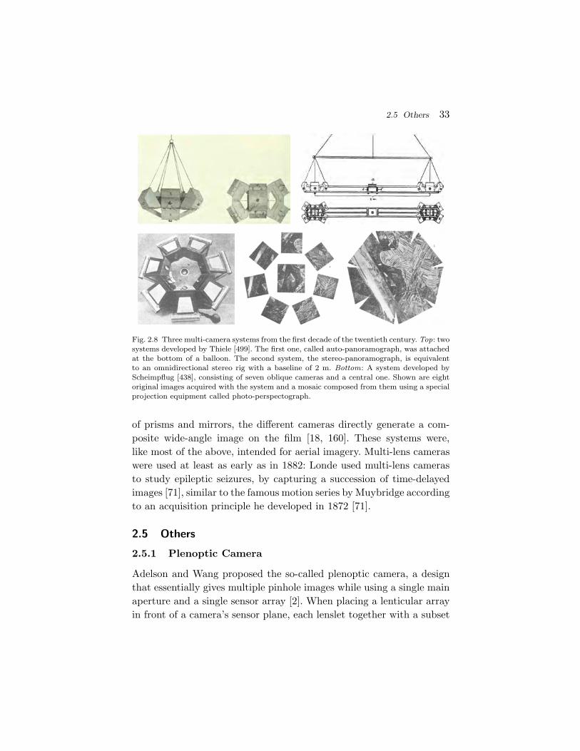
Fig. 2.8 Three multi-camera systems from the first decade of the twentieth century. Top: twosystems developed by Thiele [499]. The first one, called auto-panoramograph, was attachedat the bottom of a balloon. The second system, the stereo-panoramograph, is equivalentto an omnidirectional stereo rig with a baseline of 2 m. Bottom: A system developed byScheimpflug [438], consisting of seven oblique cameras and a central one. Shown are eightoriginal images acquired with the system and a mosaic composed from them using a specialprojection equipment called photo-perspectograph.

of prisms and mirrors, the different cameras directly generate a com-posite wide-angle image on the film [18, 160]. These systems were,like most of the above, intended for aerial imagery. Multi-lens cameraswere used at least as early as in 1882: Londe used multi-lens camerasto study epileptic seizures, by capturing a succession of time-delayedimages [71], similar to the famous motion series by Muybridge accordingto an acquisition principle he developed in 1872 [71].

2.5 Others

2.5.1 Plenoptic Camera

Adelson and Wang proposed the so-called plenoptic camera, a designthat essentially gives multiple pinhole images while using a single mainaperture and a single sensor array [2]. When placing a lenticular arrayin front of a camera’s sensor plane, each lenslet together with a subset

34 Technologies

of the sensor array’s pixels forms a tiny pinhole camera. That pinholecamera effectively only captures rays entering the camera’s main aper-ture within a subregion of the aperture, as opposed to regular cameras,where each pixel integrates light rays from all over the aperture. Con-ceptually, a plenoptic camera thus corresponds to a multi-camera sys-tem consisting of cameras arranged on a planar grid. Acquired imagescan be used to perform stereo computations or various computationalphotography tasks. We will not consider plenoptic cameras further inthis article since they are not usually used for panoramic imaging,although in principle nothing would prevent to use them with fish-eye lenses (besides the drop of spatial resolution for the already low-resolution individual pinhole sub-cameras).

More information on plenoptic cameras and similar designscan for example be found on http://en.wikipedia.org/wiki/

Integral photography and in [429, 162] The concept of plenopticcamera is highly related to that of integral imaging [323] and paral-lax stereogram [248] or panoramagram [249].

2.5.2 Biprism

A single-lens stereo system using a biprism rather than a mirror, thatdirectly produces rectified images, has been developed by Lee et al.[303].

2.5.3 Spherical Lens and Spherical Image Area

Krishnan and Nayar proposed an omnidirectional sensor consisting ofa transparent sphere, around which sensing elements are uniformlyarranged on a spherical surface, with free space between neighboringelements [290]. Hence, individual sensing elements can see through thetransparent sphere and other sensing elements, to perceive the scene.The design goals of the system are an omnidirectional field of view witha single center of projection and uniform spatial resolution.

2.5.4 Krill-Eye

Hiura et al. proposed an optical arrangement for wide-angle imagingsystem, termed krill-eye, that is inspired by compound animal eyes [228]

2.5 Others 35

The system consists of gradient refractive index (GRIN) lenses alignedon a spherical surface. Hiura et al. proposed a theoretical study onimage quality and focusing properties and built a proof-of-conceptprototype.

2.5.5 Rolling Shutter Cameras

Meingast et al. and Ait-Aider et al. studied the case of rolling shutterCMOS cameras, where the image area is not exposed simultaneously,but in a rolling fashion across rows of pixels [10, 171, 340]. The conse-quence is that when taking a picture of a moving object, it will appeardistorted. Meingast et al. developed projection models for the generaland several special cases of object motion and showed how optical flowcan be modeled [340]. They also addressed the calibration of the sensor.Ait-Aider et al. used the rolling shutter’s apparent drawback to developan approach that computes both, the pose of a known object and itsinstantaneous velocity, from a single image thereof [10]. There is a con-ceptual link to pushbroom cameras, as follows, highlighted in a similarfashion in [171, 340]. An alternative way of looking at the rolling shut-ter phenomenon is to consider a static object and a pushbroom cameramoving around it with a velocity that combines the inverse velocityof the object and a motion that compensates the difference in poseassociated with different rows of pixels in the camera.

The effect of rolling shutters was also taken into account by Wilburnet al. who built a multi-camera array with CMOS cameras [529, 530],with several applications such as synthetic aperture imaging or allowingto acquire videos with increased frame rate, dynamic range, resolution,etc. A method for calibrating such a camera array was proposed byVaish et al. [516].

3Camera Models

In the following, we review a certain number of camera models thatwere proposed in the literature. Some of them are based on physicalmodels, others are of a more algebraic nature.

These models can be described and sorted according to various crite-ria. A first characteristic concerns the spatial distribution of the camerarays along which a camera samples light in the environment. Most mod-els have a single optical center through which all camera rays pass. Wealso speak of central camera models. For these, the back-projectionfunction (see below) delivers the direction of the camera ray. Non-central camera models do not possess a single optical center. Inthat case, the back-projection operation has to deliver not only thedirection but also the position of a camera ray, e.g., some finite pointon the ray. We will also use Plucker coordinates to represent camerarays. Special cases of non-central cameras are oblique camera, whereno two camera rays meet [390] and axial cameras where there existsa line that cuts all camera rays. A special case of this are x-slit ortwo-slit models where there exist two lines that cut all camera rays.This is for example the case for linear pushbroom cameras [197].

A second property of camera models and one we would like to stressparticularly, concerns how global or local a model is. The following

36

37

definitions have already been introduced in Section 1.1, cf. also Fig-ure 1.1. Most models have a small set of parameters and in addition,each parameter influences the projection function all across the field ofview. We call these, global models, since they hold for the entire fieldof view/image area. Second, there exist several more local models,e.g., models with different parameter sets for different portions of theimage. These models have usually more parameters than global ones,but have a higher descriptive power. Finally, at the extreme, we havediscrete models, where the projection or back-projection function ismerely sampled at different points, e.g., sampling the back-projectionfunction at every pixel. These models have many parameters, one set ofthem per sampled location. They are sometimes called non-parametricmodels, but we do not find this entirely appropriate, since they do haveparameters; hence the proposed name of discrete models. Let us notethat the transition from global to local to discrete models is not dis-continuous: some local models have the same parametric form as globalones, and to use discrete models, one usually needs some interpolationscheme, for example to be able to back-project any image point, notonly sampled ones. In that respect, discrete models plus, such as inter-polation scheme, are actually local models in our language.

Many of the global and discrete models described in the followingare well known. This is less true for the local models, although theymay represent a good compromise between tractability (numberof parameters, stability of calibration) and generality. We wouldlike to point out the work of Martins et al. [331], which is ratheroften cited but often described only partially or not appropriately.They proposed three versions of the so-called two-plane model, seeSections 3.1.3 and 3.2.1 for more details. These foreshadowed severalimportant contributions by others, mostly achieved independently.First, it contains one of the first proposals for a local camera model(the spline-based version of the developed two-plane model). Second,it sparked works on discrete camera models, where camera rays arecalibrated individually from images of two or more planar calibrationgrids [85, 189], an approach rediscovered by [191, 477]. Third, thelinear and quadratic versions of the two-plane model, when writtenin terms of back-projection matrices, are nothing else than particular

38 Camera Models

instances of rational polynomial models; they are thus closely relatedto the division and rational models explained by Fitzgibbon [145]and Claus and Fitzgibbon [98] or the general linear cameras of Yuand McMillan [559], as well as others, which found a lot of interestrecently. Martins et al. may also be among the first to explicitly uselifted coordinates (cf. Section 1.2) in camera models.

Finally, a third main property of camera models we consider is thatsome models have a direct expression for forward projection, others forback-projections, some work easily both ways. This is important sinceforward and back-projections are convenient for different tasks: forwardprojection for distortion correction of images and bundle adjustment,back-projection for minimal methods for various structure-from-motiontasks, such as pose and motion estimation.

A few more general notes and explanations of notations follow.Back-projection versus forward projection. One defines the

other but one or the other may be more difficult to formulate alge-braically. For example, the classical radial distortion model is writtenusing polynomials; even with only one distortion coefficient, the poly-nomials are cubic, making it cumbersome to write the inverse model.This model is traditionally used for back-projection although someresearchers used the same expression for forward projection. Otherpolynomial models are also used for either direction.

Generally speaking though, back-projection is often easier to for-mulate. This is especially true for catadioptric systems, where back-projection comes down to a deterministic “closed-form” ray-tracingwhereas forward projection entails a search for which light ray(s) emit-ted by a 3D point gets reflected by the mirror(s) into the camera.Also, when using rational polynomial functions in point coordinatesto express camera models, this is straightforward for back-projection;using such a model for forward projection, results in general in curved“camera rays”, i.e., the set of 3D points mapped onto an image point,form a curve, not a straight line (cf. Section 3.1.8 on the cubic cameramodel by Hartley and Saxena [210]).

For these and other reasons, we will emphasize back-projectionformulations in the following. Another reason for this is that back-projection is less often used in the literature although it enables to

39

clearly formulate several structure-from-motion tasks and epipolargeometry.

Back-projection will be formulated in two different ways, either bygiving expressions allowing to compute two points on a camera ray, orby directly giving the Plucker coordinates of the ray. As for the firstcase, one of the two points on the ray will be its point at infinity andthe other, a finite point, denoted by

Bi and Bf ,

respectively. The point at infinity will be given as a 3-vector, the finitepoint as a 4-vector, both in homogeneous coordinates. Note that in thissurvey we do not consider the possibility of camera rays that lie com-pletely on the plane at infinity; such a case is of small practical interestand if necessary, all formulas are easy to adapt. Plucker coordinates ofcamera rays will be written as

Bl.

They can of course be easily computed from the two points Bi and Bf ,cf. Section 1.2.

The reason for using both expressions for back-projection is thatthe two-point expression is better suited to formulate pose estimation,whereas the Plucker-based expression allows to formulate motion esti-mation and epipolar geometry in a straightforward manner. When wedeal with central camera models, we will only give the point at infinityBi of camera rays, i.e., their direction, always assuming that camerasare in canonical position, i.e., with the optical center at the origin.

Whenever possible, we try to write the back-projection operationusing back-projection matrices, operating on (lifted) image point coor-dinates. We will use full back-projection matrices

Bl

of size 6 × n, that map image points to camera rays in Plucker coordi-nates, and partial back-projection matrices

Bi

of size 3 × n, that map image points to camera ray directions. Thevalues of n for different models depend on which liftings of imagecoordinates are required.

40 Camera Models

Finally, let us note that the back-projection for a true camera usu-ally gives rise to a half-line in 3D; many camera models do not takethis fully into account and only model back-projection via infinite lines.We do the same in this monograph and, for ease of language, use theterm ray or camera ray to denote a line of sight of a camera.

Radial distortion. In this section, models are presented in differ-ent forms, depending if they are backward or forward ones, or onlymodel radial distortion or more general distortions. Radial distor-tion models are given in different forms; they are defined by a 1D(un)distortion profile or (un)distortion function, mapping radial dis-tances in the distorted image (distances of image point to distortioncenter) to either radial distances in the undistorted image or the inci-dence angle between camera rays and the optical axis.

We use the following notations. The radial distance is denotedby rd (in distorted images) and ru (in undistorted images). The anglebetween a camera ray and the optical axis is denoted by θ. Radialdistortion models are usually given as a mapping between any of thesethree entities. For simplicity, we always assume in the following thatthe radial distortion center is equal to the principal point and thatit is known and located at the origin. When considering a distortioncenter different from the origin, the given back-projection equationscan be modified in a straightforward manner, by preceding them withthe translation bringing the distortion center to the origin. Whenconsidering a distortion center different from the principal point, themodifications of back-projection equations are equally straightforward.Whereas in the following, we suppose that the perspective back-projection consists merely in “undoing” the focal length, consideringa distortion center that is different from the principal point, requiresa full perspective back-projection.

Extrinsic parameters. Camera pose, or extrinsic parameters,is straightforward to take into account. As for back-projection,translations and rotations can be applied as follows (cf. Section 1.2):

Bf �→(

R t0T 1

)Bf

3.1 Global Camera Models 41

Bi �→ RBi

Bl �→(

R 0−[t]×R R

)Bl.

3.1 Global Camera Models

3.1.1 Classical Models

By “classical models”, we mean those used most often in applicationsand academic research, i.e., the pinhole model, affine camera models,and pinhole models enhanced with classical terms for radial and tan-gential distortions.

Pinhole model. The pinhole model, or perspective projection,assumes that all camera rays pass through a single point, the opti-cal center and that there is a linear relationship between image pointposition and the direction of the associated camera ray. That relation-ship can be expressed via a so-called calibration matrix which dependson up to five intrinsic parameters:

K =

fu s x0

0 fv y0

0 0 1

,

where fu respectively fv is the focal length measured in pixel dimen-sions, horizontally respectively vertically, s is a so-called skew termwhich may for example model non-rectangular pixels or synchroniza-tion errors in the image read-out, and (x0,y0) are the coordinates of theprincipal point, the orthogonal projection of the optical center onto theimage plane. The linear relation between image points and ray direc-tions can be written as:

q ∼ KBi.

The model is equally easy to use for forward and back-projections.In what follows, we will assume square pixels, i.e., s = 0 and fu =fv =f :

K =

f 0 x0

0 f y0

0 0 1

. (3.1)

42 Camera Models

Affine models. We also briefly mention affine camera models, wherethe optical center is a point at infinity. Various submodels thereofexist, often called orthographic, weak-perspective, and para-perspectivemodels, going from the most specific to the most general affinemodel [13, 232]. These models can give good approximations of pin-hole cameras in the case of very large focal lengths or if the sceneis shallow in the direction of the camera’s optical axis as well as farfrom the camera. Back-projection is slightly different from the pinholemodel in that the direction is the same for all camera rays (the directioncorresponding to the optical center) and the essential back-projectionoperation is thus not the computation of the ray direction, but of afinite point on the ray.

Classical polynomial distortion models. The pinhole model hasbeen enhanced by adding various terms for radial, tangential, and otherdistortions. The most widely established models are described for exam-ple in [63, 64, 149, 152, 451]. The usual model for combining radial anddecentering distortion (one type of tangential distortion) is:

xd = xd − x0

yd = yd − y0

r2d = x2

d + y2d (3.2)

xu = xd + p1(r2d + 2x2

d) + 2p2xdyd + xd

n∑i=1

kir2id

yu = yd + 2p1xdyd + p2(r2d + 2y2

d) + yd

n∑i=1

kir2id ,

where n is the number of radial distortion coefficients used. Thedistortion corrected image points correspond to a pinhole model, i.e.,are related to camera ray directions by:

Bi ∼ K−1

xu

yu

1

.

In the above model, it is assumed that the radial distortion center coin-cides with the principal point. Other models exist that consider them asdistinct and/or include additional distortion terms, see e.g., [149, 215].

3.1 Global Camera Models 43

If we neglect tangential distortion and suppose that image coordi-nates are centered in the distortion center and that the latter is equalto the principal point, then we can deduce, from Equation (3.2), theradial (un)distortion function:

ru = rd

(1 +

n∑i=1

kir2id

). (3.3)

This relates the distance of a point from the distortion center, beforeand after distortion. From this, it is easy to extract the relationshipbetween the radial distance in the distorted image and the incidenceangle of the camera ray with the optical axis:

θ = atanru

f= atan

rd

(1 +

∑ni=1 kir

2id

)f

, (3.4)

which depends on the focal length of the camera.Let us now consider a radial distortion with a single coefficient k1.

We can write down the camera ray direction in the following form:

Bi ∼ K−1

xd + k1xdr

2d

yd + k1ydr2d

1

∼

(xd − x0)(1 + k1r

2d)

(yd − y0)(1 + k1r2d)

f

∼ Bi3×10L3(qd),

where the lifting operation L3(·) is given in Equation (1.4) and theback-projection matrix is:

Bi∼

k1 0 k1 0 −3k1x0 −2k1y0 −k1x0 1 + k1a 2k1x0y0 −x0(1 + k1c)0 k1 0 k1 −k1y0 −2k1x0 −3k1y0 2k1x0y0 1 + k1b −y0(1 + k1c)0 0 0 0 0 0 0 0 0 f

,

with a = 3x20 + y2

0, b = x20 + 3y2

0 and c = x20 + y2

0.Since the first and third columns are equal, as well as the second

and fourth ones, we may use a more compact back-projection matrixof size 3 × 8:

Bic ∼

(k1 0 −3k1x0 −2k1y0 −k1x0 1 + k1a 2k1x0y0 −x0(1 + k1c)0 k1 −k1y0 −2k1x0 −3k1y0 2k1x0y0 1 + k1b −y0(1 + k1c)0 0 0 0 0 0 0 f

),

44 Camera Models

which operates on lifted image coordinate vectors of the form:

q31 + q1q

22

q21q2 + q3

2q21q3

q1q2q3

q22q3

q1q23

q2q23

q33

.

If we assume a known principal point (equal to the distortion centerhere) and translate image points such that the principal point lies atthe origin, then the back-projection equations reduce further to:

Bic ∼

k1 0 0 0 0 1 0 0

0 k1 0 0 0 0 1 00 0 0 0 0 0 0 f

,

which can be compacted similarly to the above:

Bicc ∼

k1 0 1 0 0

0 k1 0 1 00 0 0 0 f

operating on

q31 + q1q

22

q21q2 + q3

2q1q

23

q2q23

q33

.

Back-projection matrices for combined radial and tangential dis-tortion models are equally straightforward to derive. Note that thisback-projection formulation allows to easily write down equations forthe epipolar geometry, cf. Section 4.2.1.

Inversion of models. Devernay and Faugeras discussed theanalytical inversion of the classical radial distortion model with onecoefficient, using Cardan’s method. This analysis was adapted by Maet al. to other variants of polynomial radial distortion models, espe-cially rational polynomials [327], cf. also Section 3.1.8. Heikkila showedhow to formulate an approximate inverse model for radial and tangen-tial distortions [215]. A more detailed and accurate inverse model wasproposed by Mallon and Whelan [330].

3.1 Global Camera Models 45

Other models and works. The standard radial and tangential dis-tortion model is a backward one, going from distorted to undistortedcoordinates. Often, the same model is also employed for forward pro-jection, see e.g., [41, 216, 525, 521], in which case the model coefficients’values will differ of course.

Many researchers have used other polynomial models for distortion/undistortion, e.g., the so-called polynomial fisheye transform (PFET)by Basu and Licardie [41], which is nothing else than a general poly-nomial relating rd and ru, including even terms. Such models were forexample applied for endoscope calibration, see [17, 204, 454, 565]. Othercalibration approaches using such models are [8, 42, 134, 148, 215, 216,274, 302, 330, 381, 436, 437, 514, 515, 521, 525, 534]. These approachesoften differ with respect to the choice of calibration object, potentiallycarrying out controlled motions to position it in front of the camera,and with respect to the strategy for estimating the unknowns (e.g., esti-mating some parameters first while keeping others at initial values).

Kolbl proposed to use a trigonometric series to model radialdistortion, in order to better condition the normal equations occur-ring in distortion estimation [283]. Several other distortion models aredescribed in [275, 276].

Shih et al. established an approach for evaluating the errors madewhen neglecting lens distortion during calibration [449]. This is afunction of the actual amount of true distortion, the number andpositions/distribution of calibration points, the amount of noise andpossibly other factors.

Very wide fields of view. It is well known that the above classicalradial distortion model is not appropriate for cameras with a very widefield of view. To see this, refer to Equation (3.4): in order to achievea hemispheric field of view (θ = 90◦), one would need rd and thus theextent of the image area, to be infinitely large. Many alternative modelsexist, described in subsequent sections.

3.1.2 Extensions for Modeling Zooming and Focusing

In [64], Brown explained that lens distortion varies with a camera’sfocus setting but that knowledge of the distortion for two focal settings

46 Camera Models

allows to interpolate the distortion for any other setting. Also, radialdistortion depends on the distance of the object to the camera. Theseeffects are rigorously proven but seem to be used relatively seldomlyin practice.

There exist various approaches for modeling zoom lenses and theinfluence of zooming on the intrinsic parameters, as well as for modelingother intricate phenomena related to camera calibration, see e.g., [11,16, 53, 70, 96, 100, 102, 128, 150, 313, 469, 531, 533, 532].

3.1.3 Two-Plane Model

Chen et al. introduced implicit camera models in computer vision[89, 90]. Their two-plane model is mostly known through the subse-quent paper by Martins et al. [331] and follow-up papers by Wei andMa [522, 524] and others. As explained in the introduction of this sec-tion, the two-plane model is rather rich in ideas, which is why it willbe covered in some detail here.

The model is defined as follows [331]. Consider two images of aplanar calibration grid, put in known positions and assume that wecan extract matches between the image and grid in both images. Sincethe grid positions are known, points on the grid actually define a 3Dcalibration object, which may be used as input to classical calibrationapproaches. The motivations for the two-plane model are to not relyon pre-defined camera models for the calibration and to handle non-central cameras. This may be achieved as follows. If we have densematches, we may compute, for each image point for which we havetwo matches, the associated camera ray, simply by computing the linespanned by the two matched grid points. This idea was fully introducedlater, by Gremban et al. [189] and Grossberg and Nayar [191]. Martinset al. did not assume dense matches; hence, in order to compute camerarays, one must have recourse to some interpolation scheme. Basically,for an image point we want to back-project, we need to determinethe corresponding points on the two grids. To do so, Martins et al.proposed three interpolation schemes to compute corresponding pointson calibration grids, from extracted matches: two global schemes (linear

3.1 Global Camera Models 47

Fig. 3.1 Illustration of the two-plane model. A1 and A2 represent the interpolation trans-formations for the two grids, affine respectively quadratic transformations for the linearrespectively quadratic versions of the model.

and quadratic) and a local one (spline-based). The global schemes areillustrated in Figure 3.1.

First version — “Linear interpolation”. The mapping betweenthe image plane and each planar calibration grid was supposed to bean affine transformation:

Xi

Yi

Zi

= Ai q,

48 Camera Models

where i = 1,2 is the index of the grid and

Ai =

Ai,11 Ai,12 Ai,13

Ai,11 Ai,12 Ai,13

0 0 Zi

,

and it is assumed that q3 = 1. Here, Martins et al. assumed that thetwo calibration grids are parallel to the X,Y plane, at known depths Zi.They stated that other cases can also be handled similarly, but did notdevelop this further.

A more proper formulation using homogeneous coordinates also for3D points, would separate the pose of the grid, parameterized by arotation and translation, from the interpolation function “inside” theplane, which can be an affine transformation (as in Martins et al.’swork) or a projective one:

Qi ∼(

Ri ti

0T3 1

)︸ ︷︷ ︸pose matrix

1 0 00 1 00 0 00 0 1

︸ ︷︷ ︸M

Ai q ∼(

Ri ti

0T2 1

)4×3

Ai q,

where Ri consists of the first two columns of Ri and M maps 2D coor-dinates on the grid plane, to 3D coordinates. The computation of theinterpolation mappings Ai (i.e., the calibration) would be carried outbetween image points and 2D points on calibration grids, instead of 3Dpoints as in the original formulation above.

The back-projection ray of an image point q can be computedfrom the two grid points Q1 and Q2 according to Equation (1.1) inSection 1.2. Let Pi =

(Ri ti

). Then:

Bl ∼(

(A2q)3P1A1q − (A1q)3P2A2q(P1A1q) × (P2A2q)

).

This expression is quadratic in the coordinates of the image point q.It is thus clear that back-projection can be written via a 6 × 6back-projection matrix:

Bl ∼ Bl6×6 L2(q) (3.5)

operating on lifted image point coordinates L2(q) (cf. Equation (1.4)).

3.1 Global Camera Models 49

In the special case of calibration planes parallel to the XY -planeand of affine transformations Ai, we get:

Bl =

0 0 0 A1,11 − A2,11 A1,12 − A2,12 A1,13 − A2,130 0 0 A1,21 − A2,21 A1,22 − A2,22 A1,23 − A2,230 0 0 0 0 Z1 − Z20 0 0 Z2A1,21 − Z1A2,21 Z2A1,22 − Z1A2,22 Z2A1,23 − Z1A2,230 0 0 Z1A2,11 − Z2A1,11 Z1A2,12 − Z2A1,12 Z1A2,13 − Z2A1,13b1 b2 b3 b4 b5 b6

,

(3.6)

where the last row is given by the vector

b =

A1,11A2,21 − A1,21A2,11

A1,11A2,22 + A1,12A2,21 − A1,21A2,12 − A1,22A2,11

A1,12A2,22 − A1,22A2,12

A1,11A2,23 + A1,13A2,21 − A1,21A2,13 − A1,23A2,11

A1,12A2,23 + A1,13A2,22 − A1,22A2,13 − A1,23A2,12

A1,13A2,23 − A1,23A2,13

.

If instead of affine transformations, projective ones are adopted forA1 and A2, then the back-projection matrix Bl has no zero coefficientsanymore.

Second version — “Quadratic interpolation”. Here, the inter-polation function between the image plane and each of the calibrationgrids, is assumed to be quadratic, and modeled by:

Xi

Yi

Zi

= Ai L2(q),

with 3 × 6 matrices Ai. Obviously, camera rays can be expressed viaa back-projection matrix operating on degree-4 liftings of the imagecoordinates:

Bl ∼ Bl6×15 L4(q).

Third version — “Linear spline interpolation”. This is a localcamera model according to our definition and will thus be explained inSection 3.2.1.

50 Camera Models

Observations. In [331] it is noted that “The basic difference betweenthis model and the pinhole model is that all lines of sight are notforced to go through the same point”. A second major difference isthat this model allows to handle non-perspective distortions that mayin principle be quite general.

The linear two-plane model is actually identical to the general lin-ear camera (GLC) model of Yu and McMillan [559], cf. Section 3.4.4,although it is formulated differently. Also, whereas the two-plane modelwas proposed in order to interpolate calibration data, the GLC wasintroduced in order to generate novel spatial distributions of camerarays, with applications for example in image synthesis.

The linear and quadratic two-plane models are particular instancesof rational polynomial camera models, which were later introducedin full generality, cf. Section 3.1.8. Also, the two-plane models maybe among the first to explicitly use lifted image coordinates in theirformulation.

Finally, as mentioned above, they inspired works on discrete cameramodels; with the possibility of getting dense matches, it is indeed natu-ral to calibrate camera rays directly for sampled image positions insteadof computing interpolation transformations, as proposed by Grembanet al. [189], Grossberg and Nayar [191], and others, see Section 3.3.

Extensions. Izaguirre et al. showed how to incorporate the cameramotion in the back-projection matrix [251]. Since we have explicitlywritten the back-projection, this can also be done easily by combiningback-projection (e.g., Equation (3.5) for the linear two-plane model)with extrinsic parameters, as explained in Equation (1.2).

The two-plane model is formulated as a back-projection; Grembanet al. proposed an approach to deduce the forward projection operation[189]. In addition, they already posed the basis for a fully ray-basedcamera calibration, which is treated in Section 3.3.

The two-plane model was further generalized by Wei and Ma in sev-eral articles, as follows. In [522] necessary and sufficient constraints werederived for the back-projection matrix to correspond to a perspectiveback-projection, i.e., when no non-perspective distortion is present.In [523, 524] the authors also modeled the forward projection, using

3.1 Global Camera Models 51

the same algebraic model but with independent parameters and esti-mation processes. There, they also investigated the epipolar geometryassociated with their camera model. The findings of [524] do not seem tobe fully general since both for the forward projection and the epipolargeometry, the existence of an optical center of the cameras seems to beassumed, whereas the considered camera model in general correspondsto non-central cameras.

It would be worthwhile to establish the conditions under which twocameras following the two-plane model, form a stereo pair, along thelines of Seitz and Kim’s study [445], see Section 3.4.2. Further, it wouldbe interesting to establish necessary and sufficient constraints on theback-projection matrices under which the camera is central.

Champleboux et al. extended the two-plane model in two respects[85]. First, by allowing the use of more than two images of calibrationplanes. Second, by modeling the function that maps image points tolines of sight, using bicubic B-splines. They applied their approach tothe calibration of cameras but also of radiographic and range sensors.

Fiala and Basu used a 1D version of the two-plane model to calibratethe radial distortion profile of catadioptric cameras [143].

Lavest, Delherm et al. used the two-plane model to calibrate zoomcameras for different zoom settings and to obtain 3D reconstructionsfrom images taken with different zoom factors but without moving thecamera [109, 300, 301].

3.1.4 Models for Slit Cameras

Consider slit image acquisition proceeding by moving a 1D perspectivecamera with a constant translational velocity while acquiring images,which are stacked together to form a 2D image, i.e., a linear pushb-room panorama (cf. Section 2.1.1 and [197]). It is obviously an axialcamera since all viewpoints lie on a straight line due to the camera’stranslational motion. In addition, all camera rays, for all acquisitions,cut the plane at infinity in the same line — the intersection of the1D camera’s view plane with the plane at infinity. Linear pushbroomcameras are thus a special case of two-slit camera, with one slit beinga line at infinity [389].

52 Camera Models

Gupta and Hartley proposed models for the linear pushbroompanorama and its multi-view geometry [197]. They showed that for-ward projection can be modeled by a 3 × 4 projection matrix, whichrelates 3D point coordinates with lifted coordinates of the correspond-ing image point. They also showed expressions for back-projection. Letus re-derive them here. Let the 1D camera be modeled by the followingback-projection operations, where q are the homogeneous coordinatesof image points:

Bf =(t1

)+

q2

q3

(v0

)∼ q3

(t1

)+ q2

(v0

)Bi =

(a 0 b

)q = q1a + q3b.

Here, the second image coordinate is assumed to correspond to theacquisition time and v gives the translational velocity of the camera; tis the optical center position at the first acquisition and vectors a andb depend on the 1D camera’s intrinsic parameters and orientation. Thelatter are constant, thus the point at infinity of a back-projected raydoes not depend on the second image coordinate (which explains thecolumn of zeroes in the second above equation).

The Plucker coordinates of camera rays may now be expressed asfollows, based on the above two equations defining Bf and Bi (cf.Equation (1.2)):

Bl =( −q3(q1a + q3b)

(q3t + q2v) × (q1a + q3b)

)

=(

0 −a 0 −bv × a t × a v × b t × b

)︸ ︷︷ ︸

Bl6×4

q1q2

q1q3

q2q3

q23

.

The geometry of more general two-slit cameras was studied byPajdla and Zomet et al. [389, 576]. Among other issues, Zomet et al.derived the forward projection equations and have shown that 3D linesare imaged as conics. Feldman et al. showed that the back-projection forthe same two-slit cameras can be expressed via a 6 × 6 back-projectionmatrix, operating on second order lifted image coordinates [139]. As will

3.1 Global Camera Models 53

be seen later (Sections 4.2.1 and 4.3), once it is established that back-projection can be written as a linear mapping operating on order-2lifted image coordinates, it follows automatically that 3D lines areimaged as conics and that there exists a fundamental matrix of size6 × 6.

Models for other slit image systems are in principle straightforwardto establish. Consider the case of a 1D camera rotated about some axis(not necessarily containing the 1D camera’s optical center). Let the axisbe the Z-axis and the optical center at the first acquisition (q2 = 0) beat position t. Further, let the intrinsic parameters and orientation ofthe 1D camera be subsumed by vectors a and b, as above for thelinear pushbroom case. Then, full back-projection operations can bewritten as:

Bf =

cos(kq2/q3) −sin(kq2/q3) 0 0sin(kq2/q3) cos(kq2/q3) 0 0

0 0 1 00 0 0 1

(t1

)

Bi =

cos(kq2/q3) −sin(kq2/q3) 0

sin(kq2/q3) cos(kq2/q3) 00 0 1

(q1a + q3b).

Here, k expresses the rotational velocity and q2/q3 the time. Due to thetrigonometric expressions in the rotation matrix, it is not possible towrite the back-projection in polynomial form though and for exampleto establish fundamental matrices.

3.1.5 Models for Central Catadioptric Cameras

Geyer and Daniilidis proposed a unifying model for single-mirror cen-tral catadioptric systems (cf. Section 2.3.1) [164, 165]. It is embodiedby a two-step projection procedure, defined by a unit sphere and a pin-hole camera, as follows (cf. Figure 3.2). First, a 3D point is mappedonto the sphere, by intersecting the sphere with the line spanned bythe point and the sphere’s center. Second, that intersection point isprojected into a (virtual) pinhole camera. Geyer and Daniilidis showedthat this model subsumes all single-mirror central catadioptric systems

54 Camera Models

Fig. 3.2 Unified central catadioptric model of Geyer and Daniilidis. Left : Projection from3D to 2D. The line joining the 3D point and the center of the sphere, cuts the sphere. Theintersection points are then projected by a virtual pinhole camera. Right : Back-projection.An image point is first back-projected relative to the virtual pinhole camera. The intersec-tions of the camera ray with the sphere are determined. The final camera rays are the linesspanned by the intersections points and the center of the sphere. For clarity, the secondfinal camera ray is shown as a dashed line.

(see Section 2.3.1 for a list of these); the center of the sphere is theeffective viewpoint of the modeled system. Note that the first step,projection onto the sphere, has two mathematical solutions; in practice,one usually knows which one to pick but when formulating multi-viewgeometry for instance, one may have to carry along both solutions. Alsonote that the virtual pinhole camera of the model is not equivalent tothe camera looking at the actual mirror in the true catadioptric system;it is just an algebraic model.

Back-projection with this model can be formulated as follows. With-out loss of generality, let us assume that the sphere is of radius 1 andcentered in the origin. Let the projection matrix of the virtual pinholecamera be given as:

M−13×3(I3×3 −t

).

Then, an image point is back-projected, relative to the virtual pinhole,as:

Bfv ∼

(t1

)Bi

v ∼ Mq.

3.1 Global Camera Models 55

The back-projection ray intersects the sphere in two points, written inhomogeneous coordinates as:(

(Mq)T(Mq)t − (tTMq)Mq ± √DMq

(Mq)T(Mq)

),

with D = (tTMq)2 − (tTt − 1)(Mq)(Mq)T. The final back-projectiondirections are then given by the first three coordinates of these twopoints (since the sphere center is the origin):

Bi ∼ (Mq)T(Mq)t − (tTMq)Mq ±√

DMq.

Due to the square root in this expression, it is in general not possibleto directly obtain polynomial expressions.1 For the special case wherethe virtual pinhole lies on the sphere though, i.e., for tTt = 1, the twodirections are:

Bi1 ∼ t

Bi2 ∼ (Mq)T(Mq)t − 2(tTMq)Mq.

This special case corresponds to para-catadioptric cameras. The firstdirection is independent of the image point q and can thus be discarded;the second one can be written via a 3 × 6 back-projection matrix Bwhich depends on M and t:

Bi2 ∼ Bi

3×6 L2(q).

Let us finally consider the usual special case where the principal pointis supposed to be known and to be the origin and the optical axisof the camera to be aligned with the mirror axis. Further, withoutloss of generality, we assume that the camera’s optical center lies onthe Z-axis. Then, M ∼ diag(1,1,k) and tT = (0,0,−1) and the back-projection becomes:

Bi2 ∼

0 0 0 −2k 0 0

0 0 0 0 −2k 01 0 1 0 0 −k2

L2(q).

1 However, Sturm and Barreto showed that polynomial back-projection expressions can beobtained by using degree-4 liftings of image coordinates [473].

56 Camera Models

The first and third columns are identical and the second one only con-tains zeroes. We can thus write the back-projection in a more compactform as:

Bi2 ∼

0 2k 0 0

0 0 2k 0−1 0 0 k2

q21 + q2

2q1q3

q2q3

q23

.

Geyer and Daniilidis analyzed various properties of catadioptric sys-tems using their model, among which the projection of points and lines,the concepts of projective duality, epipolar geometry, etc. Barreto andAraujo proposed a modified version of this model and used it to studyvarious geometric properties, especially those related to line images andtheir application for calibration [25, 28, 29]. Mei and Rives proposedto extend the model by adding classical terms for radial and tangentialdistortion [339].

A similar model was previously proposed by Smith et al. [453]. Theirtwo-step model is defined by an arbitrary quadric surface, an effectiveviewpoint and a direction for an orthographic projection. A 3D point isfirst mapped onto the quadric surface by intersecting the line spannedby the point and the effective viewpoint, with the quadric. The inter-section point is then orthographically projected to give the final imagepoint. In practice, Smith et al. assumed that the quadric’s highest point,in the direction of the orthogonal projection, lies above the effectiveviewpoint; the orthographic projection of the effective viewpoint itselfis also considered as a distortion center. The final model used by Smithet al. has four parameters and it can model non-radially symmetricsystems. It subsumes central para-catadioptric cameras as well as thedivision model (cf. Section 3.1.8) but not hyper-catadioptric cameras.

Ying and Hu proposed another extension by replacing the spherewith a general quadric of revolution [550]. One of the quadric’s foci ischosen as effective viewpoint. The projection of a 3D point is modeledin two steps analogous to Geyer and Daniilidis’ model: the line spannedby the 3D point and the effective viewpoint is cut by the quadric. Thetwo intersection points are then projected into a virtual pinhole camerawhose optical center is located on the mirror’s revolution axis. This

3.1 Global Camera Models 57

gives the two theoretical images of a 3D point. Back-projection followsthe inverse procedure. Ying and Hu showed that this model, besidescentral catadioptric cameras, also subsumes some fisheye models, suchas stereographic projection (cf. Section 3.1.7) and the division model.A similar extension was proposed by Barreto, who showed that whenreplacing the sphere with a paraboloid, one may represent the divisionmodel [26, 27].

Bayro-Corrochano and Lopez-Franco rewrote the model of Geyerand Daniilidis in terms of conformal geometry and gave the correspond-ing formulas for forward projection of points and lines and the back-projection of image points [44]. Tolvanen et al. expressed the model ofGeyer and Daniilidis in terms of Clifford algebra [507]. Perwass andSommer proposed a model similar to Geyer and Daniilidis’, expressedin geometrical algebra terms; it subsumes the para-catadioptric anddivision models [399].

3.1.6 Non-central Catadioptric Cameras

Consider any non-central catadioptric system. Even if everything isknown about the system, i.e., the shape of the mirror, the calibrationof the camera looking at it as well as the relative camera–mirror pose,forward projection is a difficult problem. As for back-projection, it suf-fices to first back-project an image point relative to the camera, to findthe (first) intersection point of the back-projected ray with the mir-ror and to reflect the ray according to Snell’s law. For some setups,back-projection may be written analytically, e.g., for spherical or cone-shaped mirrors.

Forward projection is much harder since it is not immediately givenat which point on the mirror the reflection happens. Again, for somecases, analytical models can be formulated but in general, there is noclosed-form solution for this problem, so researchers have proposed tosolve it by non-linear optimization. One possibility is for example tooptimize the desired image point coordinates, where the cost functionis the distance between the back-projected and reflected ray, and the3D point whose projection is sought. Another possibility is to optimizethe reflection point on the mirror, using for example a similar cost

58 Camera Models

function: the distance between the camera’s optical center and the linejoining that point and the 3D point, after reflecting that line in themirror.

The special case of quadric-shaped mirrors was investigated byGoncalves and Araujo who showed how to formulate the problem viathree polynomials and to reduce it to an optimization in a single vari-able [179]. Vandeportaele also characterized the problem using poly-nomials and studied the number and nature of roots for the generalas well as special cases of quadric-shaped mirrors [517]. Agrawal et al.contributed similar results for different types of quadric-shaped mirrorsas well as for the case of cameras looking through refractive spheres [5].

3.1.7 Fisheye Models

Classical models. Several models were suggested for fisheye lenses(or rather, the opposite: fisheye lenses are constructed in order to satisfysuch models) [48, 146, 226, 350, 536] — stereographic, equiangular,2

sine-law, and equi-solid angle projection:

rd = k tan(θ/2)

rd = kθ

rd = k sinθ

rd = k sin(θ/2).

Their back-projection equations are given in Table 3.1 (where the coef-ficient k is replaced by f to homogenize notations). We observe thatstereographic back-projection can be written using polynomials; it canbe written via a 3 × 4 back-projection matrix operating on lifted imagecoordinates (here, we suppose that the principal point is known andlocated at the origin) and that it is (not surprisingly) equivalent to theback-projection of para-catadioptric cameras. The other three modelsdo not have back-projection expressions in terms of polynomials.

In [146], Fleck compared these models with respect to several cri-teria, among which the maximum theoretical field of view and light

2 This is more often called equidistant model, but in the context of back-projection, weprefer to use the word equiangular.

3.1 Global Camera Models 59

fall-off. The stereographic model is preferred by Fleck, due to represent-ing a good compromise between field of view, light fall-off, and a goodapproximate local preservation of Euclidean shapes. It seems thoughthat most fisheyes are designed to approach the equiangular model,which is thus the model used most often for fisheye camera calibration.

Hall et al. for example used an equiangular model for a fisheye lens-based imaging system used for robot guidance [80, 382, 383].

An experimental evaluation of some of the above fisheye models fora particular camera was performed by Schneider et al. [439].

As a sidenote, let us remark that interestingly, some ofthe first scientific applications of fisheye lenses concerned thearea of forest management (see http://en.wikipedia.org/wiki/

Hemispherical photography), where they were already used in the1950s. Researchers in agricultural and forestry departments came upwith calibration methods, independently from photogrammetrists. Forexample, Clark and Follin used the equiangular model for fisheyes [94].Their application was forest management and panoramic images wereused for assessing light interception and leaf areas in forests. Therefore,they were interested in images with equi-area properties, i.e., where thearea of an image region is proportional to the solid angle of the corre-sponding field of view. In [94], they assessed how well different fisheyelenses approach this property.

Other models. Various other models were proposed for fisheyelenses, or lenses with a wide field of view in general, some of themaiming at subsuming several of the above classical models.

Herbert proposed the following alternative model for fisheyecameras [219]:

rd = θ +5∑

i=1

ai siniπ θ

θmax,

where θmax is the camera’s field of view (assumed known).Various fisheye lens designs and some performance characteristics

were presented by Kumler and Bauer [294]. They used the followingmodel:

rd = k sin(βθ),

60 Camera Models

which encompasses the sine-law and equi-solid angle models shownabove. Also, if β is very small, this model approaches the equiangularone.

A similar general model was proposed by Gennery [161]:

rd =sin(βθ)

k cos(max(0,βθ)).

For β = 1 this gives the pinhole model, for β = 0.5 stereographic pro-jection, β = −0.5 gives equi-solid angle projection, and β = −1 thesine-law projection. As β approaches zero, this model approaches theequiangular one. Gennery suggested to couple this model (which sub-sumes ideal fisheye models) with a classical polynomial distortionmodel. Gennery’s full model includes also the position of the effec-tive optical center along the optical axis, as a function of θ or rd; hisfull model is thus a non-central one (an axial model to be precise) andresembles in that respect that of Tardif et al. [491], see Section 3.3.2.Besides this effect, Gennery also included the orientation of the opticalaxis relative to the image plane, in order to model non-perpendicularity.

Yet another similar model was suggested by Bakstein andPajdla [23], who used a combination of the stereographic and equi-solidangle models, depending on four parameters:

rd = atanθ

b+ csin

θ

d.

Basu and Licardie proposed a distortion function called fisheyetransform (FET) [41], inspired by the work of Schwartz on the geometryof the human visual system [441]:

rd = s log(1 + λru)

ru =erd/s − 1

λ.

Although it is called fisheye transform, this model does not handlefields of view of 180◦ or higher.

Devernay and Faugeras proposed the FOV model (field-of-viewmodel) [113]:

ru =tan(rd ω)2tan ω

2.

3.1 Global Camera Models 61

According to their description, the model is equivalent to the equiangu-lar model. However, this seems to be the case only for particular valuesof the parameter ω (cf. Figure 3.4(c) in Section 3.5). If we includethe focal length of the perspective projection in the model, we get thefollowing expression for the back-projection angle θ:

θ = atantan(rdω)2f tan ω

2.

For

f =1

2tan 12ω

the FOV model becomes equivalent to the equiangular model:

θ = rdω.

Like Gennery (see above), Devernay and Faugeras suggested to com-plement their model (or other fisheye models) by additional terms, e.g.,the classical polynomial radial distortion model, to calibrate cameras.

3.1.8 Polynomial and Rational Polynomial Models

Most of the models in the previous section were based on trigonometricfunctions, whereas polynomial expressions were used in the classical dis-tortion models of Section 3.1.1. The two-plane models of Section 3.1.3were also embodied by polynomials. In this section, we review severalother polynomial-based models.

A first possibility is to model radial distortion using polynomials,but instead of relating the distorted and undistorted radial distances asin Equation (3.3), one considers the relation between distorted radialdistances and incidence angles between camera rays and the opticalaxis:

rd =n∑

i=1

ciθi. (3.7)

This model was for example used by Herbert [219], Xiong andTurkowksi [539], Kannala and Brandt [266], Kannada et al. [267], Yinget al. [553], and Stehle et al. [459]. Kannala and Brandt further added

62 Camera Models

non-polynomial terms to account for tangential distortions [266]. Theyalso showed an approximation of the inverse (backward) model. Notethat the model in Equation (3.7) subsumes the equiangular model,which corresponds to using only the first coefficient c1.

The reciprocal is of course also possible, i.e., models of the form:

θ =n∑

i=1

ci rid .

This was used for example by Inoue et al. where a 12-th degree poly-nomial was found to be suitable to calibrate a fisheye converter [245].

Beauchemin et al. proposed a polynomial model, but wherepolynomials relate polar image point coordinates before and afterdistortion, instead of Cartesian ones [46, 47]. Their model consistsof two polynomials, one for the radial distortion function (distancefrom distortion center), one for the radial angle, capturing tangentialdistortions.

Hellmeier as well as Remy et al. used splines to model the 1D dis-tortion function [218, 427].

Rational polynomials for radial distortion. Finally, severalresearchers have proposed models based on rational polynomials, asfollows.

Fitzgibbon and independently, Brauer-Burchardt and Voss, pro-posed the so-called division model, which has one distortion coeffi-cient c [145, 62]. Before this, that model was already used by Lenz andTsai [305, 306] (see also the textbook [253, 254] by Jahne); however,they used it as forward model, i.e., in the below equations, one wouldswap the forward and back-projection equations. The division modelas defined by Fitzgibbon and Brauer-Burchardt and Voss, is given as:

ru =rd

1 − cr2d

rd =

√1 + 4cr2

u − 12cru

.

A nice feature is that the model has a closed-form inverse.The division model can be generalized by using general rational

polynomials to relate ru and rd, as proposed by Ma et al. [327]. Rational

3.1 Global Camera Models 63

polynomials were already used before the introduction of the divisionmodel, e.g., by Hellmeier [218].

Micusik and Pajdla [346] and Micusik [344] used a similar model forthe relation between image distance rd and the angle between opticalaxis and camera rays, instead of the relation between image distancesin distorted and undistorted images, as above. Their model has twoparameters and is of the form:

θ =ard

1 + br2d

.

It is in some sense a division model for the equiangular fisheye model,which it extends. Like for the equiangular model, expressing back-projection directions involves trigonometric functions; hence, Micusikand Pajdla proposed to linearize their back-projection model using aTaylor development in order to perform an initial estimation of themodel parameters during (self-)calibration.

Rational polynomials for full back-projection models. Insteadof using rational functions to model the 1D distortion function, asabove, one may use them for the actual back-projection mapping, asforeshadowed by the two-plane methods of Chen and Martins et al.[89, 90, 331] (see Section 3.1.3) and fully introduced by Claus andFitzgibbon [98]. In general, one may write general mappings betweendistorted and undistorted image points:

La(qu) ∼ M Lb(qd),

where the matrix M would contain the coefficients of homogeneous poly-nomials relating the lifted coordinates in the distorted and undistortedimage planes (for full generality, we assume that different liftings maybe possible, i.e., a �= b). We speak of rational polynomial models heresince “undoing” homogeneous point coordinates involves divisions ofcoordinates.

It is more common though to use this kind of model directly for theback-projection mapping of distorted image points to back-projectiondirections or rays:

Bi ∼ Bi Lb(qd), (3.8)

Bl ∼ Bl Lb(qd). (3.9)

64 Camera Models

In practice, Claus and Fitzgibbon used a bi-quadratic such model forcentral cameras, i.e., b = 2 and Bi of size 3 × 6 [98]. It is easy to see thatthis encompasses the division model as well as the para-catadioptricand stereographic models. Note that in order to represent the classicalradial distortion model, higher order liftings are required (cubic in thecase of a single distortion coefficient, cf. Section 3.1.1).

Let us also note that the two-plane models of Chen and Martinset al. (see Section 3.1.3) are instances of rational polynomial back-projection models.

It may be worthwhile to study which instances of the models (Equa-tions (3.8) and (3.9)) correspond for example to radially symmetric,central, perspective, or otherwise special camera models.

Rational polynomial forward models. Rational polynomialmodels are usually either applied for the back-projection function asproposed by Claus and Fitzgibbon [98], or for the 1D radial undis-tortion function as proposed by Ma et al. [327]. Hartley and Saxenaalso proposed a rational camera model, but for the forward projectionfunction [210]: the image point coordinates are expressed via ratio-nal polynomial functions of the 3D point coordinates (Hartley andSaxena used cubic polynomials). In the general case, this correspondsto curved camera rays, i.e., the set of 3D points that get projected ontothe same image point, form a curve. Hartley and Saxena showed thatthis model is a good fit for SAR cameras. It also subsumes “linear”cameras such as perspective and linear pushbroom ones, although fit-ting it to data obtained from these may lead to overfitting due to astrong overparameterization.

Essentially the same approach seems to be in routine use to modelsatellite imagery, cf. [147]. In Section 11.3 of that reference, the gen-eral term of “replacement sensor models” is employed to denote anycamera model that replaces a rigorous, physics-based, model by empir-ical expressions. The most used ones are rational polynomial functions,much like in the above works.

Hall et al. proposed the RTcam (rational tensor camera model)[200]. It essentially proceeds by first transforming 3D points via bi-quadratic rational functions, followed by a perspective projection to a

3.1 Global Camera Models 65

2D image plane (the full RTcam model is defined for arbitrary dimen-sions of scene and image). Together, the two imaging steps still cor-respond to bi-quadratic rational functions. Similar to the GLC model(see Section 3.4.4), the development of the RTcam is mainly motivatedby applications in stylized, or non-photorealistic, rendering.

3.1.9 One-Dimensional Radial Models

Thirthala and Pollefeys formally introduced so-called 1D radial cameramodels [500, 501]. They hinge on the existence of an optical axis anda center of distortion. Planes containing the optical axis are calledradial planes and lines going through the distortion center, radial lines.The only main assumption about the projection function is that all3D points in a radial plane are imaged to points on a same radialline. This effectively allows completely arbitrary radial distortions, andespecially, does not require any radial symmetry of the distortion (thedistortion “function” may be different for each radial plane–line pair)and it allows for non-central projections.

To make the model tractable, a second assumption is used though,namely that the projection can be modeled by a 2 × 4 projectionmatrix, mapping 3D points onto radial lines, represented by two homo-geneous coordinates. In other words, it is assumed that there exists aprojective relationship between the pencil of radial planes in 3D andthat of radial lines in the image. Thirthala and Pollefeys showed thatquadrifocal tensors can be formulated based on these projection matri-ces, and used for self-calibrating cameras. In general, no matching con-straints exist for less than four images. However, for the case of purerotational camera motion, a trifocal tensor exists and can also be usedfor self-calibration.

One-dimensional radial models have actually been used somewhatimplicitly before, especially embodied within the radial alignment con-straint (RAC) of Tsai [515], used also in other works [468, 106]. Tsaiproposed a camera calibration approach for cameras with radial dis-tortion, where one of the initial steps concerns the estimation of thecalibration grid’s pose relative to the camera. At this stage, it isassumed that the camera follows a 1D radial model and that the

66 Camera Models

distortion center is known. Compared to the general model of Thirthalaand Pollefeys, Tsai further assumed that angles between radial lines andassociated radial planes are identical (e.g., he had to know the aspectratio). Using these assumptions, the radial plane associated with eachextracted calibration point can be computed. One may then estimatethe pose of the calibration grid using the constraint that with the cor-rect pose, each point on the grid, must lie in the radial plane of thematched image point. It is clear that the pose cannot be fully com-puted: any translation along the optical axis will still satisfy the aboveconstraint. Hence, 5 degrees of freedom are computed, from a minimumof 5 point matches.

A 1D radial model assumption was also used in the calibrationapproach of Hartley and Kang [209]. In the initial step, they used thisto compute the distortion center from the image of a calibration grid;see more on their approach in Section 5.1.2.

3.1.10 Neural Networks

The projection or back-projection function has also been modeled andcomputed using neural networks, see for example [9, 7, 535, 577]. This isan interesting approach since it is inherently flexible and can be appliedto calibrate various kinds of cameras with various types of distortion.

3.2 Local Camera Models

3.2.1 Two-Plane Model

The third version of the two-plane model proposed by Chen andMartins et al. [89, 90, 331] (cf. Section 3.1.3) is a local camera model.Here, for each of the two calibration images, the extracted matchesdefine triangulations of the image and calibration grids respectively, cf.Figure 3.3. Back-projection is now modeled separately for each pair ofmatching triangles, by an affine transformation as in the first version ofthe two-plane model, computed from the matches associated with thethree triangle vertices. To back-project an image point, the followingis done. For each calibration image, the triangle into which the imagepoint falls is determined. A point on the calibration grid is computed

3.2 Local Camera Models 67

Fig. 3.3 Illustration of a local two-plane model (cf. text). For the second image, the trian-gulation is shown only partially.

via the affine transformation associated with that triangle. This is doneseparately for both calibration images/grids. The back-projected cam-era ray is then computed by spanning the line between the points onthe two calibration grids.

3.2.2 Warping-Based Models

Very similar to the two-plane approach is the following idea. Whereasthe two-plane model interpolates 3D points on calibration grids, thefollowing methods perform an interpolation in the image domain. Theycan all be applied with a single image of a grid, as for the correction ofnon-perspective distortions.

68 Camera Models

The general idea is as follows: consider one calibration plane andan image thereof, as well as matches between the plane and the image.Consider any warping scheme that maps the acquired image into the“ideal” image of the calibration plane (let’s say, a texture map ofthe plane). Since the ideal image is distortion-free (it is a perspec-tive image), this warping thus removes non-perspective distortions.If we determine the parameters of this warping using the acquiredimage, we may then apply it to any other image and thus remove itsnon-perspective distortions. This gives images which are distortion-corrected, i.e., images as acquired by some perspective camera. How-ever, we don’t yet know the associated perspective camera. Still, whenacquiring and then warping one or more images, the resulting imagescorrespond to images acquired by the same perspective camera. Thisenables the application of any algorithm valid for perspective cameras,to these images. For example, if images of a calibration grid are acquired(be it planar or three-dimensional), any classical perspective calibra-tion algorithm may be applied to calibrate the virtual camera. Thesame holds true for self-calibration. The complete calibration of thetrue camera is then the combination of the warp, with the computedperspective (self-)calibration.

Several methods following this general idea were proposed; theymostly differ in the choice of interpolation scheme which is required towarp entire images (the role played by the piecewise affine warp in thetwo-plane method). Without going into details, we cite the approachesof Green et al. [186], Goshtasby [182], Yokobori et al. [557], Brandet al. [59, 60], and Jackowski et al. [252]. Peuchot and Saint-Andre [401]and Bogner [54] also mentioned the feasibility of this type of approach.The method of Jackowski et al. corrects for color non-linearities inaddition to geometrical distortions [252].

Sagawa et al. used the same idea and combined it with a structuredlight-type approach in order to get dense matches between the imageand the calibration grid (a flat screen) [433], an approach used also forexample by Grossberg and Nayar, Tardif et al. and Dunne et al. (seeSection 3.3). From dense matches, the distortion-corrected image canbe constructed pixel-by-pixel instead of requiring piecewise warps andan interpolation scheme.

3.2 Local Camera Models 69

It seems somewhat surprising that apparently, none of the aboveworks went through the last obvious step to obtain a complete cameracalibration. Namely, given these distortion-corrected, hence “virtual”perspective images, one may apply any calibration approach for pinholecameras to calibrate the perspective part of the projection in additionto the non-perspective one. Such approaches were proposed previously,but only in combination with a plumb-line type distortion correctionbased on classical polynomial distortion models, see e.g., the work ofGrosky and Tamburino [190]. Dunne et al. seem to be the first to com-bine the above generic distortion correction with a subsequent pinholecalibration [125]. They also used a structured-light type approach toget dense, per-pixel, matches between calibration grids and images; dueto the per-pixel nature of the approach, we consider it in the discreteclass of models and describe it in the next section.

Comment. All approaches in this section are valid for central cam-eras only since they are based on the idea of (bijective) warps ofdistorted images into perspective ones. The two-plane approach ofSection 3.2.1 is in some sense a non-central counterpart.

3.2.3 Other Local Models

Qiu and Ma proposed an approach that is similar in spirit to the warp-based ones described above [410]. They used as input an image of a 3Dcalibration object, as opposed to a planar grid as in most other simi-lar approaches. From 2D-to-3D matches, they then seemed to computea best-fit perspective projection matrix for that image and projectedthe 3D calibration points using it. The result will constitute the idealimage onto which the distorted input image will be warped, for dis-tortion correction. Input to the next step of calibration are the imagesof calibration points in the distorted image and in the ideal image,respectively. The goal is then to compute distortion functions ∆x and∆y such that: (

xd

yd

)=(

xu + ∆x(xu,yu)yu + ∆y(xu,yu)

).

70 Camera Models

In [410], the distortion functions were estimated at a regular latticeof image pixels using non-parametric regression, and extended to thewhole image by linear or nearest-neighbor interpolation.

As mentioned above, Qiu and Ma used a 3D calibration object andfitted a perspective projection matrix to the 2D-to-3D matches. Theapproach could easily be adopted to using a 2D calibration grid: thenone may directly use the model of the grid as ideal image, such as inmost other similar approaches or, one may compute the best-fit homog-raphy (instead of projection matrix) between the 2D-to-2D matchesand use it to project the calibration points into an ideal image that is“closer” to the actual input image. The rest of the approach would bestrictly identical.

Ragot proposed a similar idea, where 3D-to-2D matches obtainedfrom an image of a calibration grid are interpolated to determine theforward respectively back-projection of generic 3D respectively imagepoints [412]. The interpolation is done within triangular tessellationsof 3D respectively image points.

Munjy proposed another very similar approach, based on the finiteelement method [359, 360]. He considered a regular triangular or rect-angular tessellation of the image plane and modeled the distortionfunction with the help of one focal length per vertex (giving the anglebetween the line of sight associated with the vertex, and the opticalaxis). Focal lengths of all other image points can then be computed viabilinear interpolation of the focal lengths of the vertices of the trian-gle/rectangle in which image points lie. The parameters of the model(principal point, focal lengths of vertices) are computed by bundleadjustment (can be done when using a calibration grid but also in fullself-calibration mode where 3D point coordinates are also optimized,using multiple images).

Lichti and Chapman extended this approach by coupling it with theclassical radial and tangential distortion terms [315]. Back-projectionis thus carried out by correcting for these classical distortions and thenback-projecting the resulting points using the local focal length com-puted from the finite-element model. Lichti and Chapman also dis-cussed correlations among the model’s parameters and how to acquireimages in order to minimize them. In [316], they further extended the

3.2 Local Camera Models 71

approach by including continuity constraints in order to overcome dis-continuities of the distortion function due to the bilinear interpolationcarried out over neighboring rectangles.

Schreier et al. [440] and Cornille [101] used a similar model, whereB-splines are used to map positions in distorted images to those inundistorted ones. They used that approach to calibrate optical andscanning electron microscopes.

Stevenson and Fleck computed a 2D distortion function that ispiecewise over a triangular tessellation of the image plane [463]. Thebasic idea is to apply an affine warp to each individual triangle such thatthe image becomes distortion-free. A notable difference with most othersimilar works is that the distortion-free image is generated with respectto stereographic projection instead of perspective, i.e., distortion-freedoes not mean as usual that straight lines remain straight (as in per-spective projection) but rather that any sphere is imaged as a circle(a property of stereographic projection). Consequently, the input areimages of spherical objects. In a first step, ellipses are fitted to theiroutlines in the images (which is an approximation, precluding the useof too large spheres). Then, the Delaunay triangulation of the cen-ters of all ellipses is computed. Let us now consider one triangle andthe associated three ellipses, centered in the triangle’s vertices. We maycompute an affine transformation that maps the three ellipses as closelyas possible into circles. This transformation is naturally only definedup to a scale change (“circle-ness” does not depend on scale). The goalis then to find a new triangulation that is consistent with the originalone, modulo these local affine transformations. This new triangulationwould be nothing else than the stereographic image of the set of spherecenters. This description does not exactly correspond to the approachtaken by Stevenson and Fleck, but transcribes its basic idea. Once thenew triangulation computed, the input image can be warped into astereographic image by piecewise warping it from the original into thenew triangulation. The result is an uncalibrated stereographic image,i.e., whose “focal length” (overall scale) is arbitrary and whose distor-tion center is unknown.

The approach is somewhat similar in spirit to the warping-basedones of Section 3.2.2, in that it results in a piecewise warp of an image,

72 Camera Models

allowing to undistort it. Differences however are the use of stereographicprojection as reference instead of perspective and that the warp isnot computed on the basis of an ideal input image (the model of a2D calibration grid), but using images of 3D primitives (here, spheres).

3.3 Discrete Camera Models

3.3.1 Ray-Based Models

As explained in the introduction to this section, most discrete cameramodels can be seen as the limiting case of the above local models,where interpolation is required in the immediate vicinity of pixelsinstead of in larger image regions. The main difference betweenthe following discrete approaches and the local ones is the explicitmotivation to calibrate individual camera rays, as opposed to forwardor back-projection mappings.

The idea of calibrating individual camera rays for discrete imagelocations was formulated by several researchers. Among the first wereprobably Gremban et al. who proposed extensions of the two-planemethod in [189] and discussed the possibility of a ray-based calibra-tion. However, they concluded that “A lookup table of calibration datafor each pixel would be prohibitively expensive”. This has to be under-stood in the historical context; such a lookup table requires four coeffi-cients per pixel, i.e., is of a size which does not pose memory problemsanymore nowadays. As alternative solution, Gremban et al. effectivelyproposed global and local camera models, based on global and localinterpolation schemes to compute camera rays for any pixel: globalschemes are based on a function that is valid for the whole image planewhereas local schemes look up the closest image points from calibrationdata (in the case of back-projection) or the closest lines of sight (in thecase of forward projection) and interpolate accordingly.

Using structured light-type acquisition setups, such interpolationscan be avoided altogether, by matching image points directly to calibra-tion points. This has been used by various researchers, e.g., Grossbergand Nayar [191], Dunne et al. [123, 124, 125], Sagawa et al. [433] (cf.Section 3.2.2), and Tardif et al. [491].

3.3 Discrete Camera Models 73

Southwell et al. proposed an idea for a structured-light typeray-based camera calibration approach [455]. The idea was to insertthe camera in a cylinder painted on the inside in smoothly varyingcolor shades such that each “point” on the cylinder has a unique color.Then, for each camera pixel, the scene point it sees can in theory beuniquely determined. Southwell et al. proposed to calibrate a cameraby generating a look-up table where for each pixel, the direction of itscamera ray is stored, after computing it from the matched point onthe cylinder. They did not use this approach in practice though, dueto practical and signal processing problems.

Grossberg and Nayar proposed a generic imaging model consistingof geometric as well as radiometric and optical parts [191]. The geomet-ric part is identical in spirit to the two-plane model and its successors.However, Grossberg and Nayar calibrated pixels individually, withoutany interpolation, using structured light-type approaches allowing todensely match images and calibration objets (e.g., flat screens). Fur-ther, instead of computing lines of sight for individual pixels, they actu-ally computed half-lines. This was mainly achieved by computing andusing the caustic of the imaging system which is used as the hull ofthe imaging system’s model, from which camera rays emanate in anoutward direction. Besides the geometric part of the imaging model, italso contains radiometric and optical aspects: for example, each pixel isassociated with individual radiometric response and point spread func-tions. Overall, a line of sight (or rather, a half-line), together with thesenon-geometric properties, make what Grossberg and Nayar termed araxel, a sort of tiny camera associated with each individual pixel of theimaging system.

Such a ray-based imaging model has been used recently by severalresearchers to devise calibration and structure-from-motion algorithms,for example by Ramalingam et al. [414, 415, 418, 477], Dunne et al.[123, 124, 125], and Goncalves and Araujo [180]. Ray-based calibrationapproaches are described in Section 5.1.2.

Debaecker et al. proposed to model the field of view of each pixelby a cone instead of a (half-)line in order to model the fact that pixelsgather a volume of light rays [108]. This may be seen as an alternativeto using a point spread function like Grossberg and Nayar.

74 Camera Models

Comments. In the above works, it is usually proposed to computeone camera ray per image pixel. Note however that this choice, whilebeing intuitive, is not the only one for a discrete imaging model. Indeed,one may compute rays for any other discrete sample of image locations.With a regular super-pixel-based sampling for example, one ray forevery n-th pixel would be computed; to compute rays for every pixel,an interpolation scheme would then be required, i.e., we are looking atlocal camera models, see the previous section. Even with a per-pixelsampling, interpolation is required to perform back-projection for everyimage point. Finally, nothing prevents in principle to apply a sub-pixelsampling for ray-based calibration. The appropriate choice of samplingdensity is a model selection question and depends on several factors,see the general discussion in Section 3.6.

3.3.2 Discrete Sampling of the Distortion Curve

Instead of computing camera rays at a discrete set of image loca-tions, which is nothing else than gathering samples of a generic back-projection mapping, one may also gather such samples for any variantof the 1D (un) distortion function: rd(θ),θ(rd), rd(ru), or ru(rd).

Most calibration approaches based on this idea then fit some globaldistortion model to these samples. Examples are some collimator-basedcalibration approaches (cf. Section 5.1.4) or an early approach for plane-based calibration by Hallert (cf. Section 5.1.2) [201].

More recent such approaches are the ones by Stevenson andFleck [462] (see Section 5.3.2), Hartley and Kang [209] and Tardif et al.[491] (see Section 5.1.2), as well as Ying and Hu [552] (see Section 5.1.1).In addition to modeling the usual 1D distortion function, Tardif et al.and Ying and Hu also considered a non-central radial distortion model:to each radial distance rd, is associated an angle θ as well as an opticalcenter on the optical axis. This is thus a radially symmetric axial model,similar to the one proposed by Gennery (cf. Section 3.1.7) [161].

3.3.3 “Isolated” Camera Rays

Grossmann et al. have considered what might be the most discretecamera model, consisting of a sparse set of pixels and associated camera

3.4 Models for the Distribution of Camera Rays 75

rays, with no requirement that rays have close-by neighboring rays [192,194]. Their proposed self-calibration approach (see Section 5.3.3) onlymakes the assumption that the camera is central.

3.4 Models for the Distribution of Camera Rays

What a camera sees of a scene depends on the light rays it captures, noton its intrinsic geometry, i.e., which pixel exactly catches the photonsof which light ray. In that respect, we may split the camera’s intrinsicparameters into two sets: one that explains which light rays the cameracaptures (these will then be considered as camera rays) and one thatexplains the mapping between camera rays and image points. To makethe distinction clearer, let us consider any two different central cam-eras, e.g., a perspective camera and a central catadioptric one. Beingcentral, both cameras catch exactly the same set of light rays: all lightrays that contain the optical center (here, we neglect of course thefinite aperture of our cameras and their different fields of view). Whatdiffers is the mapping from image locations to rays and consequencesthereof (e.g., non-perspective distortions and the spatial/angular res-olution profile). On top of this come the extrinsic parameters, tellingthe global orientation and position of the camera, or in other words, ofits set of camera rays.

In this section, we summarize several works which are primarilyconcerned with the first part of the “intrinsic geometry” of cameras,namely a description of which rays a camera captures: the locus, or spa-tial distribution, of camera rays. Several taxonomies and computationalmodels have been proposed in the last years [390, 405, 445, 472, 559].The main motivation of these works is to reason on the spatial distribu-tion of camera rays; the mapping between rays and image points is ofsecondary importance although some of these works also propose sucha mapping in order to obtain a full camera model.

3.4.1 From Central to Oblique Cameras

Cameras may be classified according to the existence of a geometricentity that is incident with all camera rays [390, 405, 472]. For a centralcamera, there exists a 3D point, the optical center, that is incident

76 Camera Models

with all rays. Any other camera is non-central. Among non-centralcameras, several subgroups exist, as follows.

In an axial camera, all rays cut some real 3D line. A special case isthe two-slit camera, where there exist two real lines that cut all rays(for example, linear pushbroom panoramas, cf. Section 2.1.1). Cam-eras falling outside any of these categories are usually termed fullynon-central or the like. A special case here are oblique cameras, forwhich any two camera rays are either identical or skew [390]. Obliquecameras are the most non-central cameras possible. A special case arelinear oblique cameras, see Section 3.4.3, for which all rays are cutby an imaginary 3D line [389] (in fact, by two conjugated imaginarylines [405]).

Other cases are cameras, whose rays are incident with a circle, as isthe case with circular non-central mosaics (cf. Section 2.1.1). Anotherexample is catadioptric camera consisting of a cone-shaped mirror anda camera located on the mirror axis. All reflected rays are incident witha circle centered in the mirror axis. However, such systems are also ofthe axial type, since all reflected rays also intersect the mirror axis.

One may define many other categories of cameras, by choosing othergeometric primitives to which all rays are incident.

3.4.2 Ray Distributions Allowing for StandardStereo Geometry

Pajdla [390] and Seitz and Kim [445] were interested in studying whichsets of camera rays admit stereo imaging conditions. What is meant bythis? To explain this, we look ahead to Section 4 on epipolar geome-try. The basic question of epipolar geometry and stereovision is, givena point in one image, which are the potentially matching points inthe other image. The answer to this is: all points whose camera raysintersect the ray of the first point. These define an epipolar curve inthe second image. Epipolar curves in the first image are defined anal-ogously. Essentially, two cameras are in standard stereo geometry ifepipolar curves in the two images are in a one-to-one relationship: thecamera ray of any point on an epipolar curve in one image cuts allcamera rays of points on the related epipolar curve in the other image

3.4 Models for the Distribution of Camera Rays 77

(for a more precise definition, see [445]). An auxiliary requirement isthat the set of epipolar curves in each image is one dimensional.

Not surprisingly perhaps, the set of rays of two cameras in standardstereo geometry, lie on a set of doubly ruled quadrics3 [390, 445]. Thetwo individual cameras then correspond to the two rulings of thesequadrics. Note that this comprises several types of non-central cameras,such as circular non-central mosaics and others [445] as well as linearoblique cameras [390].

This result concerns the locus of camera rays and is independentof the mapping from rays to image points. What it implies is that forany two cameras in standard stereo geometry, the acquired images maybe warped into images where epipolar curves are horizontal lines andmatching epipolar lines have the same vertical coordinate. In otherwords, it is possible to rectify images and then apply any standardstereo algorithm.

3.4.3 Linear Oblique Cameras

Pajdla studied the case of linear oblique cameras, already mentionedabove [390]. A defining characteristic of these is the existence of a lineartransformation that maps each 3D point to the unique camera raycontaining that point. Pajdla showed that all linear oblique camerasare projectively equivalent to the one defined as follows: the cameraray containing a 3D point (X,Y,Z,W )T is spanned by that point andthe point with coordinates (Y,−X,W,−Z)T.

This defines the set of camera rays in a linear oblique camera.In order to get a full camera model, including the mapping betweenrays and image points, Pajdla proposed to use a plane as reference. Letq be the homogeneous 2D coordinates of a point in the reference plane(the image plane if one likes). Each point inside the plane is mappedto a 3D point by some 4 × 3 pose matrix M:

Q ∼

X

Y

Z

W

∼ Mq.

3 For central cameras, this is the pencil of epipolar planes.

78 Camera Models

The camera ray is then spanned by Q and the second 3D point, definedabove. It is easy to prove that the camera ray can be written as:

Bl ∼ BlL2(q),

with Bl a 6 × 6 back-projection matrix depending on M, operating onlifted image point coordinates. The back-projection matrix is always ofrank at most 4.

For example, if we choose the following pose matrix:

M =

1 0 00 1 00 0 00 0 1

,

which corresponds to choosing the XY -plane as reference plane, thenone obtains the following back-projection matrix:

Bl ∼

0 0 0 0 −1 00 0 0 1 0 00 0 0 0 0 −10 0 0 0 1 00 0 0 −1 0 0

−1 0 −1 0 0 0

. (3.10)

We may see that, similarly to what was shown for the classicalradial distortion model (cf. Section 3.1.1) or para-catadioptric cameras(cf. Section 3.1.5), the back-projection matrix may be compacted. Thesecond column only contains zeroes and the first and third ones areidentical. Hence, back-projection for linear oblique cameras may bewritten as:

Bl ∼

0 0 −1 00 1 0 00 0 0 −10 0 1 00 −1 0 0

−1 0 0 0

q21 + q2

2q1q3

q2q3

q23

.

3.4 Models for the Distribution of Camera Rays 79

Observation. Linear oblique cameras are actually subsumed by thelinear two-plane model of Chen and Martins et al. (cf. Section 3.1.3): itis easy to prove that the back-projection matrix of Equation (3.10) canbe obtained from the one of the two-plane model (cf. Equation (3.6))by an appropriate choice of affine transformations A1 and A2.

3.4.4 General Linear Camera Model (GLC)

Yu and McMillan proposed the so-called General Linear Camera model(GLC) [559, 558], which parameterizes the set of camera rays by affinetransformations of three basis rays. Concretely, they adopted a two-plane parameterization of rays (see also a paper by Gu et al. [196] onthis parameterization) as follows. The three basis rays are given bypoints:

Ai =

ui

vi

01

Bi =

si

ti11

,

where we assume that the two planes are Z = 0 and Z = 1. All otherrays are then given by two parameters α and β, defining points in thetwo planes via affine transformations of the basis points parameterizedby two scalars α and β:

A =

αu1 + βu2 + (1 − α − β)u3

αv1 + βv2 + (1 − α − β)v3

01

B =

αs1 + βs2 + (1 − α − β)s3

αt1 + βt2 + (1 − α − β)t311

.

Yu and McMillan showed that this model allows to generate theset of camera rays of several imaging geometries, such as pinhole andorthographic cameras but also non-central cameras such as some two-slit ones. It also allows to generate less classical imaging geometries,called by Yu and McMillan the pencil camera, the twisted orthographiccamera, and the bilinear camera.

Like for linear oblique cameras, the initial main motivation of theGLC model is to propose a model for the locus of camera rays, notnecessarily a full camera model. For linear oblique cameras, a way to

80 Camera Models

get such a full model, mapping image points to rays, was shown above.As for the GLC, a natural choice is to consider the two parameters α

and β as 2D image coordinates. Before going further, let us replace theimage coordinates by homogeneous ones such that:

q ∼α

β

1

.

Then:

A ∼(u1 − u3)q1 + (u2 − u3)q2 + u3q3

(v1 − v3)q1 + (v2 − v3)q2 + v3q3

0q3

B ∼

(s1 − s3)q1 + (s2 − s3)q2 + s3q3

(t1 − t3)q1 + (t2 − t3)q2 + t3q3

q3

q3

.

Finally, the camera ray, spanned by A and B, can be written viathe following 6 × 6 back-projection matrix, operating on lifted imagecoordinates L2(q):

Bl =

0 0 0 u1 − u3 − s1 + s3 u2 − u3 − s2 + s3 u3 − s3

0 0 0 v1 − v3 − t1 + t3 v2 − v3 − t2 + t3 v3 − t30 0 0 0 0 −10 0 0 v1 − v3 v2 − v3 v3

0 0 0 u3 − u1 u3 − u2 −u3

b1 b2 b3 b4 b5 b6

.

(3.11)

For the sake of conciseness, the coefficients bi are not shown here; theycan be easily computed if necessary.

Observations. We see that the rays in a GLC can be modeled by aquadratic rational camera model, cf. Section 3.1.8. Furthermore, bycomparing the back-projection matrices of the GLC and the linearversion of the two-plane model (Equation (3.6) in Section 3.1.3), weobserve that they have exactly the same form. It can indeed be proventhat the two models are equivalent. This is maybe not surprising sinceboth models are based on affine transformations in two reference planes,although they are parameterized in different ways. Whereas the moti-vation for developing the two-plane model of Chen and Martins et al.

3.4 Models for the Distribution of Camera Rays 81

was to interpolate between calibration data, Yu and McMillan wereaiming at developing novel camera geometries. Compared to works onthe two-plane model, Yu and McMillan carried out an in-depth studyof the modeled camera geometries.

Other considerations on GLCs. In [560], Yu and McMillan gavea projection equation for a special case of GLCs (concretely, a transfor-mation that maps each 3D point to the ray it lies on in the GLC). Theyalso showed how to relate two GLCs which differ in the choice of imageplane. Whereas for perspective cameras, corresponding points in twodifferent image planes (but with the same optical center) are related bya homography, this relationship is a quartic rational function for theconsidered special case of GLCs. In the general case of GLCs, this rela-tion will be even more complicated. However, if parallel reference planesare used, then changing the distance between them does not matter:for any GLC with a particular distance between the planes, there is anequivalent GLC defined with planes separated by another distance.

The GLC model is defined by three basis rays. An extension tomultiple basis rays was proposed and analyzed for up to six rays, byPopescu et al. [406].

3.4.5 Linear Families of Lines

Ponce proposed to model the set of camera rays by two-parameter lin-ear families of straight lines, either degenerate reguli (rank-3 families)and non-degenerate linear congruences (rank-4 families) [405]. Thisframework subsumes the GLCs of Yu and McMillan [558, 559] andthe linear oblique cameras of Pajdla [390]. Ponce gives formulas forprojection, back-projection, and epipolar and multi-view geometry, for-mulated such that the two parameters of the considered linear familiesof camera rays are considered as image point coordinates. The back-projection matrix is of size 4 × 6 for two-slit cameras and linear obliqueones, and 5 × 6 for the “pencil cameras” of Yu and McMillan [559].All models subsumed by Ponce’s formulation can be expressed by6 × 6 back-projection matrices, leading to 6 × 6 fundamental matrices(cf. Section 4). Batog et al. generalized the theoretical framework

82 Camera Models

of [405] by characterizing all admissible maps that allow to model linearcameras, i.e., cameras whose rays form a linear family of lines [43].

3.4.6 Caustics

Roughly speaking, the caustic of an imaging system is the surfaceenveloping the set of camera rays, i.e., it is tangent to all rays. Caus-tics are an excellent tool to analyze properties of imaging devices, asnicely advocated by Swaminathan et al. [484]. A caustic provides onepossible description of a viewpoint locus of a camera, i.e., a point setsuch that any camera ray goes through at least one of the points inthe set (ideally through exactly one). For a central camera, the causticdegenerates into a point and for axial ones, into a line segment. Thecaustic allows to study “how central” a camera is, i.e., how much itsextent deviates from a single point. Swaminathan et al. showed howto compute the extent and shape of the caustic for axial catadiop-tric systems based on conic-shaped mirrors and such that the camera’soptical center lies on the mirror axis [484]. They showed how to usethis analysis to determine a best approximation of a single viewpoint,useful for example for approximate perspective view generation. Theyalso analyzed how resolution varies across the image area, and recipro-cally, proposed an approach to compute a mirror profile that satisfiesa desired resolution profile. Finally, the parametric form of the causticfor a class of catadioptric sensors is used in a calibration approach,described in Section 5.3.2.

Usually, to each image point corresponds exactly one point on thecaustic. This corresponds to the “viewpoint” associated with that imagepoint. To compute the entire camera ray, one still needs its direction.For axial systems, it can be easily computed since the camera ray mustpass through the axis and also be tangent to the caustic. For fully non-central systems, the full determination of camera rays requires a secondmap (of directions), besides a map from image points to the caustic.

3.5 Overview of Some Models

In Table 3.1, some of the models seen in this section are summarized.Note that in the table, we do not always use the same notation for these

3.5 Overview of Some Models 83

Tab

le3.

1.B

ack-

proj

ecti

onan

dfo

rwar

dpr

ojec

tion

equa

tion

sfo

rso

me

cam

era

mod

els.

Nam

eof

mod

elB

iθ(r

d)

ru(r

d)

Pi

rd(θ

)r

d(r

u)

Per

spec

tive

1

00

01

00

0f

at

anr

d fr

d

f

00

0f

00

01

fta

nθ

ru

Cla

ssic

alra

dia

ldis

t.

k

01

00

0k

01

00

00

0f

q3 1

+q1q2 2

q2 1q2

+q3 2

q1q2 3

q2q2 3

q3 3

at

anr

d(1

+k

r2 d)

fr

d(1

+kr2 d)

Req

uir

esso

luti

onof

cubic

equat

ion

Par

a-ca

tadio

ptr

ic

0

2k0

00

02k

0−

10

0k2

q2 1

+q2 2

q1q3

q2q3

q2 3

at

an2

kr

dk2

−r2 d

N/A

Req

uir

esso

luti

onof

quad

rati

ceq

uat

ion

Div

isio

n[6

2,14

5]

0

10

00

01

0kf

00

f

q2 1

+q2 2

q1q3

q2q3

q2 3

at

anr

df(1

+k

r2 d)

rd

1+

kr2 d

N/A

N/A

N/A

Mic

usi

k,Pajd

la[3

44]

N/A

rd

f(1

+k

r2 d)

N/A

N/A

N/A

N/A

Ste

reog

raphic

0

2f0

00

02f

0−

10

0f2

q2 1

+q2 2

q1q3

q2q3

q2 3

2a

tan

rd f

N/A

N/A

fta

n(θ

/2)

N/A

Equ

idis

tant

/-an

gula

rN

/Ar

d fN

/AN

/Af

θN

/ASin

e-la

wN

/Aas

inr

d fN

/AN

/Af

sin

θN

/AE

qui-so

lid

angl

eN

/A2a

sin

rd f

N/A

N/A

fsi

n(θ

/2)

N/A

Fis

hey

etr

ansf

orm

[41]

N/A

atan

er

d/

k−

1f

N/A

N/A

klo

g(1

+f

tan

θ)

N/A

Her

ber

t[2

19]

N/A

N/A

N/A

N/A

θ+

∑5 i=

1a

isi

niπ

θθm

ax

N/A

Kum

ler

and

Bau

er[2

94]

N/A

asi

nr

d fk

N/A

N/A

fsi

n(k

θ)

N/A

FO

Vm

odel

[113

]N

/Aat

anta

n(k

rd)

2f

tan

k 2

tan(k

rd)

2ta

nk 2

N/A

N/A

1 kat

an(2

ru

tan

k 2)

Bak

stei

nan

dPajd

la[2

3]N

/AN

/AN

/AN

/Ak1ta

nθ k2

+k3si

nθ k4

N/A

Gen

ner

y[1

61]

N/A

N/A

N/A

N/A

sin(β

θ)

kcos(

max(0

,βθ))

N/A

84 Camera Models

models as in the previous sections; rather, we try to homogenize nota-tions by naming coefficients of camera models k or k1,k2, . . .. Further,parameters akin to the focal length are denoted by f .

The shown models are all radial distortion models; their equationsare given under the assumption that the distortion center is identicalto the principal point and located at the origin. How to relax theseassumptions is outlined in the introduction to this section.

The table contains six different ways of modeling the imaging trans-formation. Cells annotated by “N/A” correspond to cases where there isno closed-form expression or, if there is no expression of back-projectionin terms of polynomials (second column).

Sample graphs of the function θ(rd) for several camera models aregiven in Figure 3.4.

3.6 So Many Models . . .

This section reviewed some camera models existing in the computervision literature. Although it is certainly not exhaustive, the list ofmodels is rather long. One may ask, which model one should chooseor recommend. For example, recurring questions are, should one use anon-central camera model for a slightly misaligned catadioptric systemor stick with a central model, or should one model fisheye lenses witha central or non-central model.

The general answer to these questions is: it depends . . .The choice of camera model depends of course on how appropriate

a model is in general for the type of camera used. For example, onewould obviously never use a pinhole model for fisheye cameras. Moreinteresting parts of the question are: how to determine the appropriateorder of a polynomial model, how to select among altogether differenttypes of models, how to decide if it is worth using a non-central modelrather than a central one, etc.

The choice of camera model or of the number of coefficients of amodel may depend on several factors:

• The amount of noise in the calibration data.• The amount of calibration data: how many images are used

and how many calibration points (or other primitives usedfor calibration)?

3.6 So Many Models . . . 85

Fig. 3.4 Graphs of the function θ(rd) for some camera models. In the first two rows, dis-tortion model coefficients k are chosen such that for rd = 1, we have θ = 90◦.

• The quality of the spatial distribution of calibration data:how well do the data cover the field of view (both across thefield of view and in depth), how good is the spatial distri-bution of the set of camera positions, how different are thecamera orientations, etc.?

• The “true” camera model: is it central or not, how pro-nounced are non-perspective distortions, etc.?

86 Camera Models

The choice depends on the combination of these and possibly otherfactors. For example, Zhang showed that the self-calibration of theclassical radial distortion model, even with a single coefficient, frommatches between images, is only stable if the actual distortion is pro-nounced and if extracted image points are accurate [566].

Let us consider extreme cases. Without noise in the data, the truemodel can be estimated without error (assuming we are not in a degen-erate situation for the position of the calibration data, such as thetwisted cubic for pinhole camera calibration [67]). Even with noise,the availability of infinitely many calibration data may allow a perfectcalibration of the true camera model.

In practice, there is noise and the number of data is finite and wemust consider the interplay of the above factors. To stress that thechoice of camera model depends on all of these factors, we may notethat even for one and the same camera, different models may be chosenfor different scenarios. For example, fisheye lenses are probably notperfectly central, i.e., not all camera rays go through a same 3D point.However, the viewpoint locus is at most as large as the aperture of thelens, i.e., a few centimeters, and in practice, much smaller. Hence, ifthe fisheye lens is used for an application where the scene of interestis meters away from the camera, then an approximation by a centralimaging model should be sufficient (unless we use many images andextremely accurate image points for calibration). However, if the scenein some hypothetical application is much less than a meter away, anon-central model may make sense.

So far, the discussion was rather qualitative. To actually imple-ment a method for choosing among camera models requires quantita-tive goodness measures.

Clearly, our question is one of model selection, for which a largebody of literature exists. The main principle of model selection is tofind a good compromise between the goodness of fit to the data and thecomplexity of a model; roughly speaking, a good model should explainthe data well but not have too many parameters. The reason for this isthat in general, a model with more parameters has a better chance to

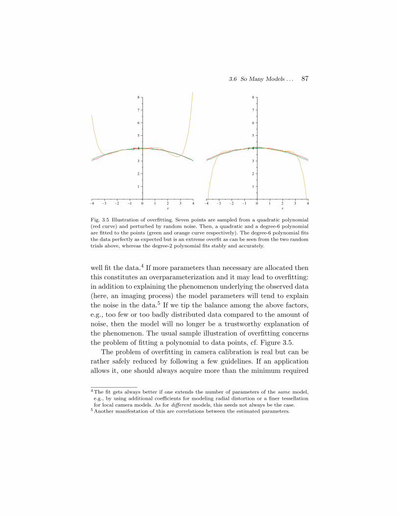
3.6 So Many Models . . . 87

Fig. 3.5 Illustration of overfitting. Seven points are sampled from a quadratic polynomial(red curve) and perturbed by random noise. Then, a quadratic and a degree-6 polynomialare fitted to the points (green and orange curve respectively). The degree-6 polynomial fitsthe data perfectly as expected but is an extreme overfit as can be seen from the two randomtrials above, whereas the degree-2 polynomial fits stably and accurately.

well fit the data.4 If more parameters than necessary are allocated thenthis constitutes an overparameterization and it may lead to overfitting:in addition to explaining the phenomenon underlying the observed data(here, an imaging process) the model parameters will tend to explainthe noise in the data.5 If we tip the balance among the above factors,e.g., too few or too badly distributed data compared to the amount ofnoise, then the model will no longer be a trustworthy explanation ofthe phenomenon. The usual sample illustration of overfitting concernsthe problem of fitting a polynomial to data points, cf. Figure 3.5.

The problem of overfitting in camera calibration is real but can berather safely reduced by following a few guidelines. If an applicationallows it, one should always acquire more than the minimum required

4 The fit gets always better if one extends the number of parameters of the same model,e.g., by using additional coefficients for modeling radial distortion or a finer tessellationfor local camera models. As for different models, this needs not always be the case.

5 Another manifestation of this are correlations between the estimated parameters.

88 Camera Models

amount of data (in terms of number of images, number of calibrationpoints, etc.). The image area should be completely covered by calibra-tion points: distortions are usually strongest, i.e., most observable atthe image border and even in the absence of distortions, a better cov-erage of the image area gives a better leverage on calibration and otherstructure-from-motion tasks (e.g., motion estimation gets stabler thewider the field of view that is effectively used). By design, calibrationgrids usually have well-distributed calibration points. One of the mostimportant aspects is that images should be taken from as different aspossible viewpoints and, crucially, with as different camera orientationsas possible. The latter aspect includes rotations about the optical axis(required if an aspect ratio is to be computed) but more importantly,one should acquire images with different directions of the optical axis(or, orientations of the image plane). Naturally, one should also spendan effort to get the most accurate image point extraction.

These are just a few general guidelines. More intricate ones whichmay be important for high accuracy calibration are that cameras shouldbest be calibrated in the same conditions as in the final application,e.g., same temperature, atmospheric conditions, even in the same ori-entation (tilting a camera may already affect its intrinsic parameters),etc. More on these issues can be found in photogrammetric literature,e.g., [336, 451].

Coming back to the model selection problem: model selection meth-ods for camera calibration were proposed for example by El-Melegyand Farag [127], Ma et al. [327], and Orekhov et al. [387]. See alsothe good discussion by Derrien and Konolidge in [111], who also evalu-ated the geometric error committed when approximating a non-centralcamera by a central model. An alternative to usual model selectionmethods is to evaluate the quality of different camera models (and ofthe estimated coefficients thereof) using other data than that used forcalibration. One possibility is cross-validation, i.e., evaluate calibrationresults using calibration images not used for calibration. Another one isto judge the quality of calibration within an actual intended applicationof the calibration: calibration is rarely a goal in its own but is carriedout in order to realize some application, such as 3D modeling or ego-motion estimation. If ground truth data for these or other applications

3.6 So Many Models . . . 89

are available, then it is obviously a good idea to measure the qualityof a calibration result via the quality of the subsequent result in theconsidered application.

A final comment is that while it is not possible to recommend this orthat camera model in general, it seems a good idea to enhance “ideal”models for cameras with large fields of view (e.g., the equiangular one),with classical radial or tangential models, as proposed for example byDevernay and Faugeras [113], Kannala and Brandt [266], Gennery [161],and Mei and Rives [339].

4Epipolar and Multi-view Geometry

Epipolar geometry is central to stereovision. On the one hand, knowingit enables to strongly constrain the problem of matching two images.On the other hand, it can be estimated from matches and then allowsfor motion estimation, self-calibration, and triangulation of 3D pointsor other geometric primitives. Epipolar geometry has been well stud-ied for perspective cameras, since the nineteenth century (see, e.g.,the excellent paper [144] by Finsterwalder on geometric foundations ofphotogrammetry, as well as modern treatments [137, 213]).

As for non-perspective cameras, much has been done in the last20 years and this section aims at giving a concise overview. It will beseen in the following that epipolar geometry is a very powerful toolfor the self-calibration of non-perspective distortions; this is based ona strong link to the plumb-line calibration approach (cf. Section 5.2.1),explained in Section 4.3.

We start the section by considering the case of calibrated cam-eras, where the epipolar geometry can be represented by an essentialmatrix. Except the question if cameras are central, non-central, axial,etc., the essential matrix is independent of the camera type. In Sec-tion 4.2, we consider the epipolar geometry of uncalibrated cameras

90

4.1 The Calibrated Case 91

and particularly, fundamental matrices for non-perspective cameras.Finally, since epipolar curves are images of straight lines (camera raysof the other camera), we consider the computation of line images inSection 4.3 and, most importantly, the above mentioned strong linksbetween self-calibration and plumb-line calibration of non-perspectivecameras.

4.1 The Calibrated Case

The epipolar geometry for a pair of calibrated central cameras can berepresented by the essential matrix E [324] and the associated epipolarconstraint on back-projected image points:

(Bi2)

T ([t]×R)︸ ︷︷ ︸E

Bi1 = 0, (4.1)

where t and R are the relative translation and rotation between the twoviews. Note that since we directly work with the directions of camerarays, the above formulation is independent of the type of central cameraand also works when considering two cameras of different types.

The essential matrix for non-central cameras was introduced byPless [402]. For non-central cameras, we must consider the completecamera rays instead of only their directions as in Equation (4.1). LetL1 and L2 be the camera rays associated with matching image pointsin a pair of views. They must intersect one another (in the 3D pointwhose images are the two matching image points). Putting togetherEquations (1.2) and (1.3) of Section 1.2, this leads to the essentialmatrix and epipolar constraint for non-central calibrated cameras:

LT2

(−[t]×R RR 0

)L1 = 0. (4.2)

The essential matrix acts on Plucker coordinates of camera rays and isthus of size 6 × 6.

In [402], Pless also gave the epipolar constraint for continuous cam-era motion. We refer to Section 6.2 for notes on the estimation ofthe central and non-central essential matrices and subsequent cameramotion estimation.

92 Epipolar and Multi-view Geometry

Sturm specialized Pless’ epipolar constraint to calibrated axial, two-slit, and central cameras, for all cases with finite/infinite slits respec-tively optical centers [472]. For axial and two-slit cameras, the essentialmatrices are of size 5 × 5 and 4 × 4, respectively. It was also shown howto establish trifocal matching tensors for these camera models.

Gasparini and Sturm showed how to derive matching tensors forline images as opposed to images of points, for central, two-slit, axial,and fully non-central calibrated cameras [158].

4.2 The Uncalibrated Case

4.2.1 Generalities

The epipolar geometry of uncalibrated perspective cameras can be rep-resented by the fundamental matrix [137, 213]. How about other centralcameras or the case of non-central ones? The answer is immediate ifback-projection can be represented as a matrix–vector product (or, bypolynomials or rational polynomials, cf. Section 3.1.8).

Central cameras. Let Bi be the back-projection matrix of a centralcamera, of size 3 × n and operating on lifted image coordinates La(q),where a and n depend on the camera model (e.g., n = 5 and a = 3 forthe one-coefficient classical radial distortion model, cf. Section 3.1.1).By plugging Bi

1 ∼ BiLa(q1) and Bi2 ∼ BiLa(q2) into the epipolar con-

straint (4.1), we directly get the fundamental matrix:

(La(q2))T (Bi)T[t]×R Bi︸ ︷︷ ︸F

La(q1) = 0.

It is of size n × n.It is of course possible to derive the fundamental matrix for two

cameras of different types with back-projection matrices of differentsizes 3 × m respectively 3 × n:

(Lb(q2))T (Bi2)

T[t]×R Bi1︸ ︷︷ ︸

F

La(q1) = 0. (4.3)

The fundamental matrix will accordingly be of size m × n.

4.2 The Uncalibrated Case 93

Due to the presence of the rank-2 skew-symmetric matrix [t]×, thefundamental matrix is always of rank smaller or equal than 2, in generalof rank 2.

Non-central cameras. The situation for non-central cameras isanalogous: it suffices to plug back-projection matrices Bl of size 6 × n

into the non-central epipolar constraint (4.2). A difference from thecentral case is that the rank of the non-central fundamental matrixdepends on the rank of the back-projection matrices as well as on therelative position of the two cameras. For example, the back-projectionmatrices of two-slit cameras are of rank 4; the rank of the two-slit fun-damental matrix is 4 if the two views are in general position, and lowerif the two views share one slit or if their slits are incident (cf. [139] andSection 4.2.2).

Epipolar curves. For perspective cameras, Fq1 represents the epipo-lar line in the second view, associated with a point q1 in the first view.In our general setting, epipolar lines are replaced by epipolar curves. Itis easy to see that the order of epipolar curves is identical to the orderof image coordinate lifting (a and b respectively in Equation (4.3)). Forexample, for liftings of order 2,3 respectively 4, epipolar curves are con-ics, cubic respectively quartic curves. This observation tells us imme-diately that for all cameras that can be modeled by back-projectionmatrices operating on second order lifted image coordinates, epipolarcurves are conics, e.g.,: linear pushbroom cameras and other types oftwo slits (cf. Section 3.1.4), linear oblique cameras (cf. Section 3.4.3),para-catadioptric cameras (cf. Section 2.3.1), the division model (cf.Section 3.1.8), all GLCs (cf. Section 3.4.4), etc. Also, epipolar curves forthe one-coefficient classical radial distortion model (cf. Section 3.1.1),are obviously cubic (cf. [566]).

As described in Section 3.4.2, non-central cameras may or may notbe in standard stereo configuration: they are, if epipolar curves in thetwo images are in a one-to-one correspondence. This is for example thecase for two-slit cameras with relative positions as mentioned above(e.g., they share a slit), which corresponds to a fundamental matrixof rank 2. Otherwise, one can still compute epipolar curves in both

94 Epipolar and Multi-view Geometry

images, but they now form 2D families in each image and are no longerin one-to-one correspondence. An algebraic consequence is an increasein the rank of the fundamental matrix, for the above example of two-slitcameras, an increase from 2 to 3 or 4.

Let us note that Rademacher and Bishop already described how tounderstand epipolar curves for arbitrary non-central images [411]. Theyalso suggested the concept of an internal epipolar geometry, i.e., anepipolar geometry of a non-central camera with itself: when consideringany ray of the camera, all other rays that cut it, are associated with anepipolar curve. For oblique cameras, no internal epipolar curves existby definition.

Epipoles. For central cameras, one may define epipoles analogouslyto the pinhole case: the image of the optical center of one camera isthe epipole in the other camera’s image plane. Further, all epipolarcurves go through the epipole. In general, there may be more than oneepipole, for example for central catadioptric cameras (see an examplein Figure 4.1) for which each 3D point is mathematically imaged in twopoints (cf. Section 3.1.5). In that case, all epipolar curves go throughall epipoles. Another example is the classical radial distortion model;

Fig. 4.1 Epipolar geometry for a perspective and para-catadioptric image pair. Cyan circlesindicate three point matches and associated epipolar lines/curves are shown in red. Epipolesare shown in white; there exist two of them in the para-catadioptric image.

4.2 The Uncalibrated Case 95

in the case of one distortion coefficient, there are three epipoles: eitherthree real points or one real and two conjugate imaginary points.

For non-central cameras, the notion of optical center and thus ofepipole does not exist anymore. However, in the special cases of axialand two-slit cameras, a weaker notion can be defined as follows: theimage of the camera axis (or axes in the case of a two-slit camera) inthe other camera gives a curve that is incident to all epipolar curves.

The non-polynomial case. The results in this section so far onlyapply to cameras whose back-projection can be modeled by matrices.In other cases, e.g., for most of the fisheye models of Section 3.1.7(cf. also Table 3.1), fundamental matrices do not exist. The epipolargeometry is still defined of course, it just cannot be expressed in theusual matrix–vector style. The epipolar geometry has been studied forsome of these cases, see the following section.

4.2.2 Existing Works

In the following, a few existing works on the epipolar geometry of non-perspective cameras are reviewed.

Classical polynomial distortion model. Zhang, in [566], studiedthe epipolar geometry of two radially distorted images and showed thatepipolar curves are cubic if only one radial distortion coefficient is con-sidered. He proposed a non-linear optimization method for estimatingthe distortion coefficients of the two images and the perspective funda-mental matrix.

Central catadioptric cameras. Svoboda et al. studied the epipolargeometry for central catadioptric cameras [482, 479, 481]. They showedthat epipolar curves are conics and gave formulas for computing theseconics, from known camera calibration and motion. They also showedthe existence of two epipoles per image, in general, which are incidentwith each epipolar conic.

Geyer and Daniilidis showed that the epipolar geometry ofpara-catadioptric cameras can be represented via a fundamentalmatrix [166]. It acts on lifted coordinates of image points and is of

96 Epipolar and Multi-view Geometry

size 4 × 4 if one assumes that images have square pixels (in the gen-eral case, it is of size 6 × 6 [471]). It can thus be estimated linearlyfrom 15 or more point matches. Geyer and Stewenius proposed a min-imal 9-point algorithm to compute the fundamental matrix betweentwo para-catadioptric cameras, based on constructing a Grobner basisof the polynomial equation system given by the point matches [172].

Geyer and Daniilidis [168] and independently, Sturm [471], showedhow to systematically derive multi-view relationships for para-catadioptric cameras. Their approaches use a direct extension of theframework used for perspective images by Faugeras and Mourrain [138]and Triggs [511]. They allow to re-derive the above para-catadioptricfundamental matrix and in addition, trifocal or quadrifocal tensors.Sturm showed that using the same framework, one may obtain multi-view relations for any combination of para-catadioptric, perspective,or orthographic images [471]. It is clear from Section 4.2.1 that thiseasily generalizes to all types of camera models represented by back-projection matrices.

Other central catadioptric cameras than para-catadioptric ones,i.e., those based on hyperboloidal or ellipsoidal mirrors, are lessnicely modeled. The main reason for this is that mathematically, eachimage point is back-projected to two camera rays (cf. Section 3.1.5).Although only one of them is physically plausible, it is not possibleto dissociate the two rays while expressing them using polynomialsin the image point coordinates. Sturm and Barreto showed that itis possible to represent the two rays by a single geometric object (aline complex) which can be represented using polynomials [473]. Thisenabled the definition of back-projection and fundamental matrices,the latter being of size 15 × 15.

Non-central catadioptric cameras. Cone-shaped mirrors usuallylead to non-central catadioptric cameras (cf. Section 2.3.1). The epipo-lar geometry for such cameras, when restricted to planar motions, wasderived by Yagi and Kawato [542]. As for two cameras mounted oneon top of the other, with aligned mirror axes, the epipolar geometry issimple [456]: the mirror axes pierce the two image planes in the epipolesand the radial lines going through the epipoles, are epipolar lines. One

4.2 The Uncalibrated Case 97

may see that this situation is always true for pairs of radially symmetricaxial cameras with aligned camera axes.

Wurz-Wessel proposed a numerical approach for computing epipolarcurves in images of free-form mirror surfaces [538].

Central and non-central panoramas. Ishiguro et al. showed thatin central panoramic images (see Section 2.1.1), 3D lines are imagedas sinusoidal curves [246, 247]. Consequently, epipolar curves are sinu-soidal too, a result also derived by McMillan and Bishop [338] and Bun-schoten and Krose [68, 69]. Torii et al. studied the multi-view geometryof central panoramas [509].

Huang et al. studied the epipolar geometry for non-centralpanoramic images generated by a perspective 1D sensor rotated aboutan axis parallel to the sensor line but not necessarily passing throughthe 1D camera’s optical center [236, 237, 238]. Further, the 1D sen-sor may be oriented such that the sensor line, the optical center, andthe rotation axis are not coplanar. Huang et al. derived the epipolargeometry for such images as well as several special cases [236, 238] andproposed motion estimation methods [237]. Sivic and Pajdla proposedan in-depth geometric study of non-central panoramic images and theirstereo configurations [450].

Menem and Pajdla established the epipolar geometry between anon-central panoramic image and a pinhole image [342].

Polynomial and rational polynomial models. Claus and Fitzgib-bon uncovered the fundamental matrix for the bi-quadratic rationalfunction model (see Section 3.1.8) [98]. It is a 6 × 6 matrix that mapslifted image points to the six coefficients (five plus a scale factor) ofthe epipolar conics in the other image. If one restricts the model to theone-parameter division model, then image lines are circles and epipolargeometry may be written via a 4 × 4 fundamental matrix [31, 98].

Barreto and Daniilidis showed that this is the case even if the twocameras have different distortion coefficients [31]. They also showedhow to compute the fundamental matrix and extract the distortioncoefficients from it. In [35], they showed that the combination of apara-catadioptric camera and one following the division model is alsosubject to a fundamental matrix.

98 Epipolar and Multi-view Geometry

Two-slit cameras. Gupta and Hartley showed that the epipolargeometry of linear pushbroom cameras can be modeled by a 4 × 4 fun-damental matrix, expressed in lifted point coordinates [197]:

(q2,1q2,3 q2,1q2,2 q2,2q2,3 q2

2,3)F

q1,1q1,3

q1,1q1,2

q1,2q1,3

q21,3

= 0,

where qj,k denotes the kth homogeneous coordinate of a point inimage j. Images of straight lines are hyperbolas and consequently, soare epipolar curves.

Feldman et al. have developed the fundamental matrix for moregeneral two-slit cameras [139]. To be precise, they considered the casewhere a two-slit image is constructed from images acquired by a per-spective camera that translates by a constant speed parallel to theimage plane, such that at each acquisition instant t, the vertical pixelcolumn at coordinate s(t) = αt + β is taken from the perspective image,where α and β can be arbitrary values. The final image is obtained byconcatenating these pixel columns. For any pair of values α and β, thisconstruction corresponds to a two-slit camera. The first slit is the lineof optical centers corresponding to the translational motion whereasthe second slit depends on the values of α and β. The two slits, whenseen along their common perpendicular, form a right angle.

Feldman et al. showed that two two-slit images constructed fromthe same original image sequence but with different values α and β

are subject to an epipolar constraint embodied by a 6 × 6 fundamentalmatrix, acting on the lifted image coordinates. They also revealed thegeneral conditions under which two two-slit images have an epipolargeometry (see also Section 3.4.2); this is the case if the two camerasshare one slit completely or if each slit of one camera intersects bothslits of the other camera. In the first case, the stereo system has a pencilof epipolar planes, in the second case, these are replaced by epipolarquadrics.

Note that even if the cameras are not in one of these configurations,there exists a fundamental matrix for two-slit images, of size 6 × 6. Itallows, as usual, to compute the epipolar curve (here, a conic) for every

4.2 The Uncalibrated Case 99

image point. However, epipolar curves in the two images are no morein a one-to-one correspondence: different points on the same epipolarcurve in one image, may be associated with different epipolar curves inthe other image.

Khan et al. showed that there exists a fundamental matrix betweena linear pushbroom panorama and a perspective image and used thisfor estimating the position of a query perspective image with respectto a set of georeferenced panoramic images [273].

One-dimensional radial camera model. Thirthala and Pollefeysshowed the existence of quadrifocal tensors for the 1D radial cameramodel [500]; refer to Section 3.1.9 for some more details.

The case of pure rotations. It is well known that two images takenby a pinhole camera undergoing a pure rotation about its optical centerare related by a homography. How about other central cameras?

We consider the case of cameras modeled by back-projection matri-ces of size 3 × n, acting on a-order lifted image coordinates. For anypair of matching points q1 and q2, we must have:

R Bi1 La(q1) ∼ Bi

2 La(q2),

where R is the rotation relating the two images. This constraint can bewritten as:

{RBi1La(q1)} × {Bi

2La(q2)} = 03,

which is equivalent to three bilinear constraints (only two being inde-pendent) on the lifted image coordinate vectors:

(La(q2))TMjLa(q1) = 0, j = 1 · · ·3,

with three matrices Mj of size n × n which depend on the rotationmatrix R and the two back-projection matrices.

There is no bijective homography in general, unlike in the pinholecase, but it is replaced by the above bilinear constraints, which allow,for any point q1, to compute all potential matches q2. In general,there are only finitely many matches. To be precise, since the matchingconstraints are linear in the lifted coordinates of q2, there are in general

100 Epipolar and Multi-view Geometry

at most a2 potential matches (two independent constraints on a-orderlifted coordinates).

As for the 1D radial camera model and the case of pure rotations,Thirthala and Pollefeys showed the existence of trifocal tensors [500,501] (cf. Section 3.1.9).

The case of planar scenes. Like for pinhole cameras, the case ofa planar scene is very similar to that of a rotating central camera. Forexample, Drareni et al. derived the expression for plane homographiesfor linear pushbroom cameras and proposed a calibration approachusing planar grids [120]. Fitzgibbon mentioned plane homographies forthe division model [145]. Sturm and Barreto showed the existence ofplane homographies for all central catadioptric cameras [473].

4.3 Images of Lines and the Link between Plumb-lineCalibration and Self-calibration of Non-perspectiveCameras

As will be discussed in Section 5.2.1, non-perspective camera parame-ters can in general be fully calibrated from images of straight lines.There is a strong link between this, epipolar geometry and self-calibration: from point matches between images, one can computethe epipolar geometry. Epipolar geometry allows to compute epipolarcurves, which are nothing else than images of straight lines (of camerarays of the respective other camera). It is thus obvious that epipo-lar geometry allows for the self-calibration of non-perspective imagingmodels, at least partially. One may even directly use any plumb-linetechnique for self-calibration: from the epipolar geometry, one maygenerate arbitrarily many epipolar curves and use these as input toplumb-line calibration. This direct link between plumb-line calibra-tion, epipolar geometry, and self-calibration is implicitly present in allnon-perspective self-calibration approaches, although it has not beenexplained before in its full generality. It will be developed further inSection 5.3.1.

Line images. As for the computation of a 3D line’s image, this isparticularly simple for cameras modeled by back-projection matrices.

4.3 Plumb-line Calibration and Self-calibration of Non-perspective Cameras 101

In the case of non-central cameras and back-projection matrices of size6 × n, operating on a-order lifted image coordinates La(q), the imageof a 3D line L is computed as follows. An image point q lies on the lineimage if its back-projected camera ray intersects the line L, i.e., if (cf.Equation (1.3)):

LT(

03×3 I3×3

I3×3 03×3

)Bl

︸ ︷︷ ︸cT

La(q) = 0. (4.4)

We immediately see that the image of L is the curve of order a whosecoefficients are given in the vector c. In the case of a = 2 for example,the line image is a conic; the six coefficients defining its symmetricmatrix representation, are contained in c. An example of a line imagein a linear pushbroom panorama is shown in Figure 4.2.

In the case of central cameras, we can obtain the analogous resultafter computing the full back-projection ray from Bf (the origin) andBi ∼ BiLa(q) (the direction of the ray):(

BiLa(q)0

)∼(

Bi

0

)6×n

La(q).

By inserting this in Equation (4.4), we compute the line image forcentral cameras as:

cT ∼ LT(

03×3 I3×3

I3×3 03×3

)(Bi

0

)∼ LT

(0Bi

).

Fig. 4.2 The image of a line in a linear pushbroom panorama.

102 Epipolar and Multi-view Geometry

Fig. 4.3 Line images for the equiangular camera model. The black curve is the image of anyline in the focal plane i.e., the plane containing the optical center and perpendicular to theoptical axis. It is naturally a circle and corresponds to the hemispheric part of the field ofview. The other curves show the images of lines whose interpretation planes (plane spannedby a line and the optical center) form angles of 70,50,30, and 10 degrees with the opticalaxis, respectively. The limiting case of 0 degrees corresponds to lines that are coplanar withthe optical axis and whose images are lines going through the distortion center. Althoughin general, line images are not algebraic curves, the parts within the hemispheric field ofview, i.e., within the black circle, can be relatively well approximated by conics.

Let us denote by l the second sub-vector of length 3 of L. This repre-sents the line at infinity of the plane spanned by the optical center (theorigin) and L. The line image can then also be written as:

cT ∼ lTBi.

Non-polynomial back-projection. In this case, line images cannotbe computed by matrix–vector products. Still, it suffices to plug intoEquation (4.4) the expression of back-projected image points to getan equation defining the line image, allowing for example to plot it.For example, Figure 4.3 shows line images for the equiangular cameramodel; the figure suggests that although they are not algebraic curves,e.g., are not conics, they can be well approximated by conics within ahemispheric field of view.

5Calibration Approaches

This section aims at providing an overview of different calibrationapproaches, mainly with respect to the type of images or other infor-mation that are used for calibration, with an emphasis on approachesdeveloped for omnidirectional cameras. The section is a far fromexhaustive treatment of the topic of calibration. A few other referencesare as follows. An excellent overview of photogrammetric calibrationapproaches and their historical development, together with the devel-opment of distortion models, is the paper [95] by Clarke and Fryer,see also a paper by Remondino and Fraser [426] and a book section byBoland [55]. Among the many books covering the topic, we may citethe Manual of Photogrammetry, its fourth edition of 1980 [451] andthe more recent fifth edition [336]. The article [430] by Roelofs is aninteresting extended account of the state of the art on calibration upto 1951. Other relevant books are [19, 195, 213, 287] to cite just a few.

5.1 Calibration Using Calibration Grids

5.1.1 Three-Dimensional Grids

This is probably the most well-known calibration approach and willnot be detailed much further. Let us just note that in order tocalibrate omnidirectional cameras, several researchers used hollow

103

104 Calibration Approaches

3D calibration objects painted with markers or patterns on the inside,such that cameras are put inside the object for calibration, see,e.g., [23, 61, 83, 413, 455, 506, 519, 552]. Usually, the object was used togather 3D-to-2D matches which could then be used like in traditionalcalibration approaches. Ying and Hu used two hemispherical calibrationobjects with different radius to calibrate a model akin to the two-planeone (cf. Section 3.1.3) [552].

Among the many other approaches, let us mention one by Shih et al.who proposed a method for calibrating one radial distortion coefficientas well as the perspective camera parameters, via the solution of an8 × 8 eigenvalue problem [448]. This is very similar to recent approachesfor the simultaneous estimation of multi-view geometry (e.g., the fun-damental matrix) and a distortion model (e.g., the division model), forexample the approaches of Fitzgibbon and Claus [98, 145] and Micusikand Pajdla [344, 346, 347, 349]. Shih et al. also gave a similar calibrationmethod for the usage of planar grids.

Bastanlar et al. developed a calibration approach for central cata-dioptric cameras that is akin to the DLT approach for pinhole cameras[40]: computation of a projection matrix from 3D-to-2D matches,followed by the extraction of intrinsic parameters. In the case of cata-dioptric cameras, the projection matrix is somewhat different from thatof a pinhole camera: as shown by Sturm and Barreto [473], it is possi-ble to formulate a projection matrix but which does not directly map3D points to 2D points, the reason being the existence of two theoreticalimage points (cf. Section 3.1.5). Instead, the projection matrix maps3D points to a degenerate dual conic, representing these two imagepoints. Besides this difference, DLT-like calibration is also possible, asexploited by Bastanlar et al. [40]. Gasparini et al. and Barreto et al.developed similar procedures for using planar grids [36, 159].

Huang et al. proposed a calibration approach for non-centralpanoramic images and compared it experimentally to a line-based anda self-calibration method [239].

5.1.2 Planar Grids

Many approaches have been developed for using planar grids incamera calibration, due to their ease of manufacture, storage, and use.

5.1 Calibration Using Calibration Grids 105

Planar or near-planar objects, e.g., crosses, are routinely used inphotogrammetry, usually via a (self-calibrating) bundle adjustmentprocedure. Computer vision researchers proposed “closed-form” typesolutions [475, 567], which are suboptimal and should be followed by abundle adjustment (cf. Section 6.4).

In this section, we concentrate on plane-based calibrationapproaches developed for omnidirectional cameras or other cameraswith general distortion profiles. There are many approaches for globalcamera models, which usually apply similar procedures: an optionalinitialization procedure, followed by a bundle adjustment. We will thusnot describe them in any more detail and refer the reader to the ref-erences on camera models in Section 3.1. As for the local models, thecalibration procedures designed for them are mostly already outlinedin Section 3.2. In the following, we give a few details on plane-basedapproaches for discrete camera models, for two variants thereof — ray-based models and discrete samples of the distortion curve.

Ray-based calibration. Several similar approaches for ray-basedor raxel-based calibration were proposed, e.g., by Gremban et al. [189],Champleboux et al. [85], and Grossberg and Nayar [191]. The principleis simple: two or more images of planar calibration grids are acquired,with a known motion of the camera or grid between the acquisitions.A dense matching between the grid in each position, and the cameraimage, is carried out. Hence, for each pixel, one can compute its cameraray by fitting a 3D line to the set of matched grid points, which canbe put in the same coordinate frame since the motion between imageacquisitions is known. This way, camera rays can be computed for eachindividual pixel (or some other spatial sampling of the image area, beit sub-pixel or super-pixel-wise).

Debaecker et al. used a similar procedure to calibrate their cone-based camera model from multiple images of planar grids [108]. Thesemethods can be considered as dense versions of the two-plane approach,cf. Section 3.1.3.

This type of approach was generalized by Sturm and Ramalingamin order to allow an image acquisition without having to know thecamera/grid motion [477]. While the approach based on the knowledgeof camera/grid motion can in theory work with two images, a minimum

106 Calibration Approaches

of three images is required in the case of unknown motion. Sturm andRamalingam showed that from matches for three images, the unknowncamera/grid motion can be recovered via the computation of particulartrifocal tensors. Once the motion is known, the above approach can bereadily applied to compute the camera rays and thus to finalize thecalibration. In [477], the minimal case of three images was considered;this was extended toward using multiple images in [418], allowing for aneasier calibration of omnidirectional cameras. Sturm and Ramalingamdeveloped several variants of their approach, for using planar as well as3D calibration grids, as well as for calibrating fully non-central [477],central [477], or axial cameras [420]. In [416], they gave a minimalsolution for the calibration of a central camera using matches for fourpixels and three grids.

Goncalves and Araujo used this approach to first compute pixel–raymatches, to which they then fitted a catadioptric model [180].

Dunne et al. used a structured-light type approach where an LCDscreen is used as planar calibration grid, allowing to achieve densematches between the grid and the image through the display of asequence of particular patterns [125]. Matches between the grid and oneof the input images are used to define a warping from the image to thegrid. The warping, when applied to that input image, will by definitionlead to a perspectively correct image of the grid — the grid itself. Thiswarping thus eliminates all non-perspective distortions. After apply-ing it to other images of grids (they do not need to be of the samegrid), one may use any calibration approach for perspective camerasto calibrate the perspective part of the camera projection, e.g., themethods of Zhang or Sturm and Maybank for planar grids [475, 567].This approach combines the ideas of warp-based approaches (cf. Sec-tion 3.2.2) and ray-based calibration.

Discrete sampling of the distortion curve. In the 1950s, Hallertdeveloped formulas for non-linearly optimizing either intrinsic or extrin-sic parameters of a camera looking at a planar grid, supposing therespective other set of parameters is known [201]. He also includedthe computation of a radial distortion model in his procedure. Themodel he used is of the discrete sampling type (cf. Section 3.3.2): he

5.1 Calibration Using Calibration Grids 107

used a calibration grid of 5 × 5 regularly distributed points and seemedto assume that the grid can be positioned such that the center pointcoincides with the distortion center. Then, he computed the radial dis-tance in the undistorted image, for every circle centered in the grid’scenter point and going through other points in the grid. From the com-puted values, he seemed to interpolate the complete distortion function,between distorted and undistorted radial distances. This is probablyone of the first examples where radial distortion is determined by com-puting samples of the distortion function, as also done for example byHartley and Kang [209] and Tardif et al. [491], see below.

Hartley and Kang proposed a set of methods for calibrating cameraswith general radial distortion [209]. Their key observation is that pointmatches between a planar calibration grid and an image with what-ever radial distortion are subject to a constraint akin to the epipolarconstraint and that the epipole in the image plane is nothing else thanthe center of radial distortion. The latter may thus be computed byfitting a fundamental matrix to the point matches and extracting theepipole from it (one may also use multiple images and fundamentalmatrices to get a better estimate). It was shown that this can also bedone, in a similar fashion, when using a 3D calibration grid or by self-calibration, i.e., from images of an unknown scene (see Section 5.3.1).Hartley and Kang then used the assumptions of a radially symmetriccamera and of a monotonic distortion curve, to compute the latter,from multiple images of grids. They showed how to compute a discretesampling of the distortion curve as well as how to fit parametric modelsthereof.

Hartley and Kang’s approach was studied experimentally byBarreto et al. for the task of calibrating endoscopic cameras using pla-nar grids [37]. It was found to be superior to using the division or aclassical model for radial distortion.

Tardif et al. proposed two approaches for plane-based calibra-tion of a general radially symmetric radial distortion model (cf. Sec-tion 3.3.2) [491]. The approach is similar in spirit to Hartley and Kang’salthough the method for finding the distortion center is less elegant.The basic versions of these approaches work for central cameras; anextension for non-central ones was also proposed.

108 Calibration Approaches

5.1.3 One-Dimensional Grids: Sticks or CircularGrids Positioned in Radial Planes

Adorni et al. proposed a calibration method for the task of back-projecting an omnidirectional image onto a fronto-parallel ground plane[3]. They made the assumption of a radially symmetric camera andacquired an image of a linear calibration object lying on the groundplane, carefully positioned such that the camera’s optical axis “pierces”the object at a known position. For each marker on the calibrationobject, the distance to the optical axis as well as the distance of theimage point from the assumed distortion center is recorded in a look-uptable. By interpolating the information contained in this look-up tableand using the assumption of radial symmetry, each image point can bemapped to the point on the ground plane that it sees, and vice versa,i.e., back-projecting the image to the ground plane is possible. A simi-lar approach was proposed earlier by Southwell et al. which instead ofmarkers on the calibration object used one with a fractal Grey codepattern printed on it [455].

As for classical cameras, i.e., non-omnidirectional ones, using stickswith markers is probably the de facto standard approach for calibratingcommercial multi-camera systems for motion capture, although manyalternative approaches exist, e.g., [33, 480]. How to calibrate a singlecamera using a 1D object, was shown by Zhang [568].

5.1.4 Calibration Grids at Infinity — Collimators, StellarCalibration, Vanishing Points

A classical photogrammetric calibration technique exploits arrays ofcollimators or devices with a movable collimator [95, 202, 269, 492].The incidence angle of each collimator with the lens to be calibrated ismeasured, e.g., using theodolites or a goniometric apparatus. One caninterpret such an array as a calibration grid lying at infinity: insteadof providing matches between image positions and 3D points, theydirectly provide directions of camera rays for image positions. If a pla-nar array is used (collimator beams are coplanar) and positioned suchthat that plane contains the distortion center, one can directly samplethe radial distortion function from the observations, or fit any radial

5.1 Calibration Using Calibration Grids 109

distortion model to them. In the case of a non-planar array, tangen-tial distortions may be measured as well. More generally speaking, onemay fit any global or local central camera model to data obtained fromcollimators.

Another classical method termed stellar calibration consisted inexploiting the well-known angular position of stars to calibrate cameras(care had to be taken though to take into account, e.g., atmosphericrefractions) [151]. This may again be seen as using a calibration gridlying at infinity.

Finally, we may mention calibration techniques exploiting vanish-ing points arising from scene structure, e.g., associated with paralleledges of buildings. Knowing the angles between the associated direc-tions in 3D gives essentially the same input as collimators and images ofstars, although usually with (much) lower accuracy. Also, the numberof vanishing points in typical scenes is low, often not higher than three.Thus, this kind of observation could typically not be used to measurenon-perspective distortions. However, from three vanishing points withknown angles, up to three intrinsic parameters of the pinhole model canbe estimated. Methods doing so are for example those by Gracie [185],Caprile and Torre [81], and Echigo [126].

Hughes et al. showed that vanishing points arising from sets of paral-lel lines may be used to calibrate the distortion center of radially sym-metric distortion models [241]. They did this for the division model(which was used as an approximation to the equiangular model), byshowing the following properties. Lines are imaged to circles and a setof parallel lines are imaged to circles which intersect in two vanishingpoints; these correspond to the two mathematical images under thedivision model, of the point at infinity associated with the set of lines.The line joining the two vanishing points also contains the center ofradial distortion. Thus, when observing at least two different sets ofparallel lines, the distortion center can be computed in a straightfor-ward manner. It seems that this approach may be used for any radiallysymmetric distortion model. In [240], Hughes et al. extended the pre-vious approach by estimating another intrinsic parameter besides thedistortion center, namely the proportionality factor k of the equiangu-lar camera model (cf. Section 3.1.7).

110 Calibration Approaches

5.2 Using Images of Individual Geometric Primitives

By individual primitives, we mean that their relative position is notknown.

5.2.1 Lines — The Plumb-Line Approach

Brown introduced the so-called plumb-line approach which allows tocalibrate non-perspective distortions from images of straight lines [64].Since then, many such approaches have been proposed for differ-ent camera models, see below. Line-based calibration approaches areattractive since they allow to separate perspective from non-perspectiveparts of the imaging model and since their algebraic complexity istypically lower than that of full calibration formulations, allowing foreasier closed-form type solutions. Further, since lines are omnipresentin urban or interior scenes or in man-made objects, they allow fora calibration in many applications where calibration grids cannot beemployed.

Classical polynomial distortion model. Kang proposed a plumb-line method where snakes that are constrained by the radial distortionmodel are used to fit to images of straight lines, thereby estimating thedistortion coefficients [263].

Alvarez et al. [14] used a classical distortion model and a plumb-linetype method, based on observations of sets of collinear points. Theydefined a cost function which measures how close undistorted pointsare from being collinear. That measure is not based on the Euclideandistance between points and lines, i.e., is an algebraic distance. How-ever, Alvarez et al. showed that it is possible to find the distortioncoefficients that are globally optimal under that measure, using a stan-dard resultant-based technique. This is possible for up to two distortioncoefficients but hints on how to possibly handle more than two are alsogiven in [14].

Many other plumb-line approaches were proposed for the classical aswell as other distortion models, e.g., [127, 240, 241, 272, 337, 408, 427,485, 503, 510, 520, 521, 553, 575]. Ricolfe-Viala and Sanchez-Salmeroncombined a plumb-line constraint with a constraint expressing the

5.2 Using Images of Individual Geometric Primitives 111

invariance of the cross-ratio of collinear points, to calibrate a classi-cal distortion model from images of planar grids [428].

Central panoramas. Smadja et al. proposed a plumb-line calibra-tion method for circular central panoramas, acquired by a 1D camerarotating about its optical center [452].

Catadioptric cameras. As for catadioptric cameras, Geyer andDaniilidis introduced a plumb-line method [164, 165, 167]. Based ontheir unified model (see Section 3.1.5), they showed that from tworespectively three images of lines, one may fully calibrate a centralhyper-catadioptric respectively para-catadioptric camera. They gavean algorithm for the para-catadioptric case; Barreto and Araujo devel-oped an algorithm for hyper-catadioptric cameras [28, 31] as well asan improved algorithm for para-catadioptric ones that is able to fullycompute the mirror shape [30, 32]. Ying and Hu, Vandeportaele et al.,and Wu et al. gave similar algorithms [518, 537, 551]. Previously, Geyerand Daniilidis also proposed a method for calibrating para-catadioptriccameras from images of sets of parallel lines [163].

It is noteworthy that central catadioptric cameras can be fully cali-brated from just images of lines, contrary to perspective cameras, withor without the classical radial or tangential distortion models. In thelatter case, images of straight lines only allow to calibrate the cam-era up to an arbitrary perspective projection, whereas for catadioptriccameras, a full calibration is possible. One explanation for this is thatcatadioptric cameras cannot be modeled by a perspective projection fol-lowed by a distortion in the image plane. Rather, the distortion alreadyhappens in the first step of the projection (in the unified model of Geyerand Daniilidis, when mapping 3D points onto a sphere). Every cameramodel for which this can be said may be fully calibrated from imagesof lines even if their relative position is unknown.

Fish-eye models. Devernay and Faugeras presented a plumb-linemethod in [113] and applied it to different distortion models: the clas-sical backward model used by Brown [64], but also the models proposedby Basu and Licardie and the field-of-view model (see Section 3.1.7).

112 Calibration Approaches

Polynomial and rational polynomial models. Claus and Fitzgib-bon proposed two plumb-line methods for the bi-quadratic rationalfunction camera model (see Section 3.1.8) [97]. They are both basedon the fact that with that model, lines are imaged as conics. Thefirst method starts with estimating conics from extracted line imagesand recovers distortion parameters via the factorization of a measure-ment matrix consisting of the matrices of all image conics. The secondmethod is of the bundle adjustment type; it estimates the distor-tion model’s coefficients using as cost function the Sampson distancebetween image points and line images (conics). Barreto as well asStrand and Hayman proposed similar plumb-line methods for the1-parameter division model, for which line images are circles [26, 466].

Discrete camera models. Tardif et al. showed how to calibrate ageneral radially symmetric radial distortion model with a plumb-lineapproach [489]. Their method is applicable to both, a parametric radialdistortion curve and a discrete sampling of it.

General remarks. Whenever the back-projection operation can bewritten using polynomials, it is easy to set up “closed-form” solutionsfor plumb-line calibration. Consider the case of back-projection matri-ces for central cameras, of size 3 × n, for any n. As we have seen inSection 4.3, the image of a line L can be written as:

cT ∼ lTBi,

where l is the line at infinity of the plane spanned by the optical centerand the line L. If we have m line images, we can set up a system like:

cT1...

cTm

∼

lT1

...lTm

Bi.

It is easy to see that the back-projection matrix can be recoveredby factorizating the matrix on the left, like in factorization-basedmethods for structure-from-motion [508]. It can only be determinedup to the pre-multiplication with an arbitrary 3 × 3 matrix, which

5.2 Using Images of Individual Geometric Primitives 113

corresponds to a projective transformation of the directions of back-projected points — the perspective part of the imaging process. Inother words, the non-perspective distortions are fully recovered. Oncethis is done, one may apply any calibration or self-calibration methoddesigned for perspective cameras, to make the calibration complete.

This approach can work with a minimum of three line images,although this is not recommended in practice; in that case, the matrixon the left of the above equation can directly be adopted as solutionfor Bi. If prior knowledge on the camera is available, i.e., if constraintson Bi are available, fewer line images may be sufficient in theory.

One may apply the same approach to non-central cameras, withmore general back-projection matrices, e.g., of size 6 × n. In that casehowever, it must be taken into account that often, they will be of ranklower than 6, a fact that has to be taken into consideration when esti-mating them.

Finally, as always, the best approach for calibration is to optimizea meaningful geometrical/statistical error criterion, possibly afterinitializing with any of the above approaches, which usually comesdown to a non-linear bundle adjustment like optimization process.For example, one may simultaneously estimate the coefficients ofundistorted lines and of camera model parameters where the costfunction is the sum of Euclidean distances between undistorted linesand points. It will in general be better even to minimize distances inthe original, distorted image, i.e., distances between original imagepoints and line images, where the latter are parameterized by cameramodel parameters and parameters for line images (two for centralcameras, four for non-central ones).

5.2.2 Spheres

Algorithms using images of spheres for the calibration of perspectivecameras were proposed for example by Penna [398], Daucher et al. [104],Teramoto and Xu [498], and Agrawal and Davis [6], to name a few.

Stevenson and Fleck used images of spheres to calibrate a localcamera model, see Section 3.2.3 [463].

Ying and Hu showed how to use sphere images for calibrating centralcatadioptric cameras [551]. In these cameras, spheres are mapped to

114 Calibration Approaches

conics, like in perspective images (to be precise, the mathematicalimage of a sphere is the union of two conics, but in true cameras onlyone of them is usually visible). Ying and Hu showed that from threeor more extracted conics, the catadioptric camera can be calibrated.Ying and Zha analyzed the relationships between sphere images andthe image of the absolute conic and proposed a linear calibration algo-rithm based on these [554, 555, 556].

5.2.3 Circles

Herbert proposed a calibration procedure where instead of pointmatches or images of lines, projections of circles painted on the insideof a hemisphere are used [219]. Coefficients of his distortion models(see Section 3.1.7) are then estimated by measuring and comparing theimaged areas of such circles.

Many algorithms using circles for calibrating pinhole cameras havebeen proposed in the literature, see [91, 199, 257, 476] to name just afew.

5.3 Self-calibration

Self-calibration has attracted great interest in the computer vision com-munity in the last close to 20 years. The possibility of camera self-calibration was already well known in photogrammetry, although itwas usually identified with the non-linear simultaneous optimizationof intrinsic and extrinsic camera parameters and scene structure (self-calibrating bundle adjustment), whereas computer vision researchersaimed at developing initialization approaches.

Most computer vision self-calibration works concern pinholecameras; a good general reference is the book by Hartley and Zisser-man [213]. In the following, we describe approaches for non-perspectivecameras.

5.3.1 Self-calibration from Image Matches

General observations. As explained in Section 4.3, there is a stronglink between plumb-line calibration (calibration from line images) and

5.3 Self-calibration 115

self-calibration. From image matches, epipolar geometry can be recov-ered; epipolar curves can be generated and since they are images ofstraight lines (camera rays) they can be used as input to any plumb-line approach. Instead of this, mainly conceptual, idea of explicitlygenerating line images from a computed epipolar geometry, one maydirectly use fundamental matrices for self-calibration.

In the following, we only consider the self-calibration of the non-perspective part of a central camera model. By this we mean thatit suffices to recover its 3 × n back-projection matrix up to the pre-multiplication by any (invertible) 3 × 3 matrix M. The effect of M isa projective transformation of the directions of back-projected camerarays, i.e., a perspective part of the camera model.

In the following, we consider the case of a fundamental matrixbetween two images taken by the same central camera. Let B beits 3 × n back-projection matrix (we omit the superscript i here forease of notation). The fundamental matrix is then given by (cf. Equa-tion (4.3)):

F ∼ BT[t]×R B.

Consider rows of F; they are linear combinations of the rows of B,with coefficients of these combinations given by the matrix (BT[t]×R).Similarly, the columns of F are linear combinations of the columns ofBT, i.e., of the rows of B. This suggests the idea of determining the rowsof B by computing a basis of the space of row and column vectors of F.To do so, let us now look at the singular value decomposition (SVD)of F:

F ∼ UΣVT,

where all matrices are of size n × n. Since F is of rank 2 in general, theSVD can be reduced by only considering the first two columns of U,the first two rows of VT and the two non-zero singular values in Σ:

F ∼ Un×2Σ2×2VT2×n.

The columns of U as well as the rows of VT are linearly dependenton the rows of B. Let us stack them together in a 4 × n matrix and

116 Calibration Approaches

compute its SVD: (UT

VT

)4×n

= W4×nΓn×nXTn×n.

In the absence of noise, the above matrix is of rank 3 in general, sinceall its rows are linearly dependent on the three rows of B. The threerows of XT corresponding to the non-zero singular values in Γ can nowbe directly adopted as the rows of the back-projection matrix B. It isclear that the rows of B are only defined up to linear combination of therows of XT, but this does not matter: as stated above, B needs only berecovered up to a projective transformation M, and this means nothingelse than a linear combination of its rows.

A more compact alternative procedure would proceed as follows.Stack F on top of FT and compute the SVD of this 2n × n matrix:(

FFT

)= UΣVT.

Using similar arguments as above, the matrix on the left is of rank 3in general and the three rows of VT corresponding to non-zero singularvalues in Σ can directly be chosen as rows of B, which concludes thisself-calibration algorithm.

A similar procedure was proposed by Claus and Fitzgibbon forthe case of 3 × 6 back-projection matrices [98]. The self-calibrationapproach for para-catadioptric cameras by Geyer and Daniilidis (cf.Section 5.3.1) follows the same principle [166, 170]. In their case, theback-projection matrix could be fully determined (up to a rotationinstead of a projective transformation), due to using constraints onthe coefficients of B. More generally speaking, there are two ways ofobtaining more than the self-calibration of “just” the non-perspectivepart of B. (i) Use constraints on the entries of B. (ii) In any case,once B is estimated up to a projective transformation, we are in thesituation of an uncalibrated perspective camera. From the fundamen-tal matrix between two perspective images, one may estimate up totwo intrinsic parameters [206, 474]; usually one just computes the focallength. Hence, in many cases it should be possible to obtain a fullself-calibration of non-perspective cameras from a single fundamentalmatrix.

5.3 Self-calibration 117

From the above, it is straightforward to extend self-calibration tothe use of multiple fundamental matrices for a better stability and/orto the self-calibration of two or more cameras with different parame-ters/models. Without giving a formal proof, it should be possible forexample, to self-calibrate three entirely different cameras (possibly withdifferent sizes of back-projection matrices), from the three pairwise fun-damental matrices. This possibility was demonstrated by Geyer andDaniilidis for para-catadioptric cameras [166, 170].

In the following, we review a few self-calibration approaches pro-posed in the literature for different types of non-perspective cameramodels.

Classical distortion model. Zhang proposed an approach for thesimultaneous estimation of one radial distortion coefficient and the per-spective fundamental matrix, by non-linear optimization of the epipolarconstraint [566]. Based on his experimental results, Zhang concludedthat the distortion coefficients can only be estimated reliably if match-ing points can be extracted accurately and if the actual distortion issignificant (cf. the discussion in Section 3.6). In other cases, the estima-tion is ill-conditioned or in other words, taking into account distortioncoefficients besides the fundamental matrix constitutes an overparam-eterization. One may further add that it seems to be required thatimage matches be well distributed across the image planes, as is alwaysrequired when estimating radial distortion, which is most observabletoward the borders of images.

In [461], Stein proposed a virtually identical method, as well as anextension to three views. Here, trifocal transfer errors are used to definea cost function which is optimized simultaneously over the distortionand trifocal tensor coefficients.

Non-central panoramas. Huang et al. proposed a self-calibrationmethod for non-central panoramic images acquired by rotating 1D cam-eras [239]. In their approach, it is required that images be obtained byrotating about the same axis.

Catadioptric cameras. Gluckman and Nayar showed how to deter-mine the focal length of the camera in a single-lens catadioptric stereo

118 Calibration Approaches

system using one camera and two planar mirrors [174, 175]. Since thissetup is identical to a system of two perspective cameras, perspec-tive self-calibration approaches can be readily applied. Gluckman andNayar used point matches between the two views and the fundamentalmatrix estimated from them. Their reported results were not perfect.We believe that this is because of a generic degeneracy: whenever thetwo mirrors are arranged in a rotationally symmetric position withrespect to the camera’s optical axis, the two virtual cameras (the realcamera reflected in the two mirrors) are in a degenerate relative posefor focal length computation [474]. In situations close to this, resultsmay be expected to be inaccurate.

The first self-calibration approach for non-perspective catadioptricsystems is probably due to Kang, who considered the central para-catadioptric case [262]. Based on an expression of the epipolar geom-etry as a function of the relative motion between two views and therelevant intrinsic parameters, he proposed a cost function consisting ofthe sum of distances between image points and epipolar circles. Thiscost function was minimized non-linearly.

Geyer and Daniilidis showed how to self-calibrate para-catadioptriccameras from point matches, via the estimation of the 4 × 4 funda-mental matrix [166, 170]. Their key observation was that the null-space of the fundamental matrix contains the vector representationof the image of the absolute conic (a circle in their case). They showedthat the fundamental matrix is of rank 2; if both images are takenby the same camera, then the left and right null-spaces may be inter-sected to find the image of the absolute conic and thus to calibratethe camera. Geyer and Daniilidis also showed that if the images aretaken with different para-catadioptric cameras, then their intrinsicparameters can be found from the fundamental matrices between threeimages. These observations can be generalized, cf. the above paragraph“General observations”.

Sturm showed that a similar concept can be used for the self-calibration of para-catadioptric cameras from homographies associatedwith scene planes [471].

In [344, 347, 349], Micusik and Pajdla proposed an approach forthe estimation of the epipolar geometry of non-central catadioptric

5.3 Self-calibration 119

cameras, demonstrated for the examples of a spherical mirror (alwaysnon-central) and misaligned para- and hyper-catadioptric systems.The approach proceeds in several steps. First, an appropriate centralapproximation to the full non-central back-projection is derived. Thisapproximate model is then linearized such that its coefficient(s) canbe estimated simultaneously with the fundamental matrix, by solvinga quadratic eigenvalue problem similarly as in Fitzgibbon’s approachfor the division model (see below). This allows to initialize and thenoptimize the complete, non-central model.

Polynomial and rational polynomial models. Fitzgibbonshowed how to simultaneously estimate radial distortion and perspec-tive multi-view relations such as the fundamental matrix, plane homo-graphies, or trifocal tensors, by solving quadratic or cubic eigenvalueproblems [145]. The approach is based on the division model (see Sec-tion 3.1.8). This was extended by Micusik and Pajdla [344, 346, 349](see previous paragraph), Barreto and Daniilidis [33, 34], Claus andFitzgibbon [98], and Steele and Jaynes [458].

Claus and Fitzgibbon showed how to estimate the coefficients of thefull bi-quadratic rational function model for central cameras (i.e., 3 × 6back-projection matrices) from point matches between two views [98].They also analyzed the nature of epipolar curves (conics) and showedhow to calibrate the model from one image of a planar calibration grid.

Micusik and Pajdla used a division-type model as an extensionto the equiangular fisheye model (see Section 3.1.7) and showed,analogously to Fitzgibbon’s approach, how to simultaneously esti-mate its two parameters and the fundamental matrix [344, 346, 349].If both parameters of their model are used, 15 point matches arerequired; for a one-parameter version 9 matches are sufficient. Theyused an analog approach to self-calibrate a one-parameter model ofpara-catadioptric cameras, leading to a quartic instead of a quadraticeigenvalue problem [344, 348, 349].

Barreto and Daniilidis showed that even if two images with differ-ent distortion coefficients for the division model are considered, theyare subject to a 4 × 4 fundamental matrix [34]. They gave an algo-rithm for linearly estimating the distortion coefficients and the epipolar

120 Calibration Approaches

geometry, from a minimum of 15 point matches. The same factoriza-tion approach is used in [33] to calibrate the nodes of a multi-cameranetwork, including radial distortion, intrinsic and extrinsic parameters.

Li and Hartley proposed a different method for estimating distortioncoefficients of the division model from point matches in two views [311,312]. They decoupled the estimation of distortion coefficients from thatof the fundamental matrix and showed how to estimate one or twocoefficients of the division model from 9 point matches.

Kukelova and Pajdla proposed a minimal method for the self-calibration problem with one distortion coefficient, using 8 pointmatches [292]. In [72, 291, 293], Kukelova, Byrod et al. gave minimalmethods for the following two problems. (i) Estimating the fundamentalmatrix together with two different coefficients for the division model,from 9 point matches (a non-minimal linear solution for this problemwas first given by Barreto and Daniilidis [34], see above). (ii) Estimat-ing the epipolar geometry and one distortion coefficient (identical forboth images) in the case of partially calibrated images (known principalpoint and square pixels); a minimal method for estimating the distor-tion coefficient and the essential matrix (as opposed to the fundamentalmatrix) was given.

Steele and Jaynes extended Fitzgibbon’s approach in two ways [458].First, they solved a more general quadratic eigenvalue problem, allow-ing to obtain less ambiguous and more accurate results in the case ofmore than the minimum of 9 point matches. Second, their approachmay be used to simultaneously estimate a global distortion coefficientand fundamental matrices for multiple image pairs, thus increasing theaccuracy of each of these estimates.

Kannala et al. proposed a bundle adjustment type approach for theself-calibration of a unified central catadioptric model (Section 3.1.5)and the polynomial model of Equation (3.7), from matches betweentwo images [267].

Discrete camera models. Thirthala and Pollefeys showed how toself-calibrate the 1D radial camera model (see Section 3.1.9) from fourimages, based on estimating the associated quadrifocal tensor [500].Their approach is stratified, starting with a projective reconstruction

5.3 Self-calibration 121

and converting it to a Euclidean one. At that stage, the radial dis-tortions of the camera are not yet calibrated, just the mapping fromradial planes to radial lines. To get a full calibration, Thirthala andPollefeys used the assumption of radial symmetry. They either fit adivision model to the reconstruction [501] or a discrete camera model.

In addition to their approaches for grid-based calibration of generalradial distortion models (see Section 5.1.2), Hartley and Kang alsoshowed that self-calibration is possible [209]. They observed howeverthat results are too unstable in the presence of even small amounts ofnoise.

Tardif et al. proposed an approach for the self-calibration of a gen-eral radially symmetric radial distortion model (cf. Section 3.3.2) fromimages of a planar scene with unknown structure [489]. A more robustextension which also works for images with different radial distortionswas presented in [490]. A factorization-based method for the same prob-lem was given by Ramalingam et al. [417].

5.3.2 Special or Known Motions

Like for perspective cameras, using special types of camera motionor actually knowing the camera motion usually allows to simplify theself-calibration problem. This enables less complex algebraic problemformulations, allows to work with fewer images, and often gives moreaccurate results. As for perspective cameras [207], the most used motionis pure rotation about the optical center; an approximate rotation is suf-ficient if the scene is sufficiently far away. In the following, we describeseveral approaches, first ones based on special types of motion (butwith unknown motion parameters), then ones using knowledge of themotion parameters.

Classical distortion model. Stein proposed a method based onpure rotational camera motion [460]. Matching (undistorted) imagepoints are related by a special homography. Distortion coefficients andthat homography are estimated simultaneously, by non-linear optimiza-tion, using a reprojection error type cost function.

Sawhney and Kumar showed the importance of estimatingnon-perspective distortion for generating mosaics based on images

122 Calibration Approaches

acquired with a rotating camera [435]. They proposed a direct method(i.e., based on image intensities rather than feature matches) for simul-taneously estimating distortions and image alignment transformations.In their work, they only considered a single term of the classical radialdistortion model, but it is obvious that other distortion models may beestimated from images taken under pure rotation.

Fish-eye models. Xiong and Turkowski performed the self-calibration of a fisheye camera from pure rotations [539]. The cameramodel they used is the extension of the equiangular model described inSection 3.1.7. The calibration is performed by non-linear minimization,where the distortion center/principal point is initialized as the centerof the image’s bounding ellipse.

Discrete camera models. Thirthala and Pollefeys showed how toself-calibrate the 1D radial camera model (see Section 3.1.9) from threeimages taken under pure rotational motion [500, 501]. To be precise,in the non-central version of the 1D radial model, pure rotation wouldrather correspond to camera poses such that all optical axes intersectin a single point. A full self-calibration algorithm was given for centralcameras.

Tardif et al. showed how to self-calibrate a general radiallysymmetric radial distortion model using either pure rotational or puretranslational camera motion [489]. They used both a parametric radialdistortion curve and a discrete sampling thereof.

The probably most general self-calibration problem considered todate, besides the work of Grossmann et al. (see Section 5.3.3), con-cerns the ray-based self-calibration of a general central camera. In thefollowing works, the only assumption made is that of continuity —neighboring image points have neighboring camera rays.

Ramalingam et al. showed that from pure translational motions,the self-calibration of camera rays is possible up to a projectivetransformation of their directions [419]. They stated that a com-plete self-calibration is possible from two rotational motions and gavean algorithm for full self-calibration from one translational and tworotational motions. In [421], they proposed an algorithm that onlyrequires two rotational motions.

5.3 Self-calibration 123

Nister et al. and Grossmann et al. [193] gave several similar results,mainly for the case of infinitesimal rotations or translations [380, 193].Their main result is an algorithm for self-calibration from rotationaloptical flow. They issued the conjecture that two infinitesimal rotationsabout different axes are sufficient for a complete self-calibration. Thiswas theoretically proven by Espuny and Burgos Gil who also gave apractical algorithm [130, 131].

Known motions. Stevenson and Fleck developed an approach usinga robot arm and a light source to calibrate a camera [462]. The cam-era is mounted on the robot arm which then rotates the camera byknown angles (the rotation should be about the camera’s optical cen-ter, although this is not further discussed in [462]). The image of thefixed light source is extracted in each frame. The approach calibrates aradially symmetric central model, as well as optical parameters such aslight fall-off across the image plane. The gist of the proposed approachis as follows. An initial estimate of the distortion center is assumed;the camera is rotated such that the light source is seen at the distor-tion center. Then, the camera is successively rotated in one directionby some small angle increment. The observed image positions of thelight source, together with the known rotation angles, directly allow toconstruct a discrete sampling of the distortion function. Stevenson andFleck also described how to correct the initial estimate of the distortioncenter.

Similar active approaches were also proposed by Du and Brady[122] and Kojima et al. [282] and seem to be in use for the calibrationof cameras for space and planetary exploration, see e.g., [334].

Swaminathan et al. proposed an approach for calibrating non-central catadioptric cameras, using image matches and knowledge ofthe camera motion [484]. The approach is based on a parametric modelfor the caustic of catadioptric cameras; its coefficients are non-linearlyoptimized in a bundle adjustment like manner.

5.3.3 Image Statistics

Farid and Popescu showed in [135] that distortion coefficients, as well ascoefficients of non-linear intensity transformations, may be estimated

124 Calibration Approaches

from single images without the use of calibration objects. This is basedon a frequency analysis of the image and on the assumption that non-linear transformations (geometric or intensity distortions) introducespecific higher-order correlations in the frequency domain. In somesense, this approach is an example of using natural image statistics, herefor camera calibration. A similar approach was developed by Yu [561].

Grossmann et al. showed that a highly discrete camera model,consisting of “isolated” camera rays (see Section 3.3.3), can be self-calibrated just by taking images of unknown scenes, based on simpleassumptions about their appearance [192, 194]. Roughly speaking, itis assumed that the smaller the angle between two camera rays, themore likely it is that the associated pixels produce similar greylevels;this is in some sense, an assumption on the statistics of natural images.When acquiring a sufficiently large set of images, observed differencesbetween greylevels of different pixels, allow to infer the topology of thecamera rays. Based on a simple off-line training, one may even recoverthe angles between rays and finally, their directions in a common coor-dinate system.

5.4 Special Approaches Dedicated to Catadioptric Systems

In this section we only cover methods that were not explained in anyof the above sections. When using catadioptric cameras, one rarelydoes not know anything at all about the shape of the mirror, unlessit is taken “off-the-shelf” or if the producer of a catadioptric cameradoes not disclose any information about the mirror’s shape. In case themirror shape is known, calibration can be considered as estimating therelative pose between camera and mirror, and possibly the camera’sintrinsic parameters. Otherwise, several possibilities exist, as explainedbelow.

Known mirror shape. One of the two (self-)calibration methodsproposed in [262] by Kang is based on the extraction of the mirror’supper circular rim in the image. From this, some or all intrinsic param-eters can be computed. This idea was used in several other works, forexample [110].

5.4 Special Approaches Dedicated to Catadioptric Systems 125

Strelow et al. proposed a calibration method using 3D calibrationgrids [467]. They assumed that the perspective camera looking at themirror is already calibrated. The calibration of the catadioptric sensorthen comes down to estimating relative mirror-to-camera pose. Strelowet al. estimated this together with the pose of the calibration grid,by non-linearly optimizing the reprojection error of calibration points.Lhuillier showed how to optimize the mirror-to-camera pose and the 3Dposition of points observed and matches in several images, via bundleadjustment [308].

Aliaga used a parabolic mirror, looked at by a perspectivecamera [12]. Hence, the catadioptric system is non-central. A calibra-tion procedure was proposed that estimates the focal length of theperspective camera and its position relative to the mirror (the orien-tation seems to be assumed to be perfect, i.e., the optical axis to beparallel to the mirror axis), as well as a radial distortion coefficient.

Similar but more restrictive approaches exist that require knowl-edge of the mirror shape and the camera’s intrinsic parameters, i.e.,calibration comes down to estimating the relative mirror-to-camerapose. Mashita et al. [332] supposed that the perspective camera is cali-brated and that the mirror’s circular upper boundary can be extractedin the image. Then, classical algorithms for estimating the pose of acircle in 3D can be applied, e.g., [114], after which the pose of theentire mirror, relative to the camera, is known. This effectively givesthe calibration of the entire catadioptric system. This is similar to theapproach by Kang described above, which was developed for centralpara-catadioptric cameras, whereas the one by Mashita et al. is forperspective cameras and central as well as non-central setups.

Another such method was proposed by Fabrizio et al. where besidesthe upper boundary of the mirror, a second circular section of it mustbe observable in the image, e.g., the footprint of a black needle gluedon the mirror of some prototypes of catadioptric systems [133]. Fromthe images of these two circles, the mirror pose is computed along withsome intrinsic camera parameters.

Unknown mirror shape. Several possibilities exist to perform cal-ibration in this case, some of which are explained in the following.

126 Calibration Approaches

If it is known that the catadioptric camera is one of the centraltypes (cf. Section 2.3.1), then one may for example use any of theunified models (cf. Section 3.1.5) to calibrate it.

A more general approach was proposed by Caglioti et al. for the casewhere all that is assumed is that the mirror is a surface of revolution[78]. The perspective camera looking at the mirror can be positionedarbitrarily and the mirror shape can be arbitrary (besides being a sur-face of revolution), hence the system is non-central in general. Theproposed calibration approach requires to extract the silhouette of themirror in the image as well as the image of at least one straight line inthe scene. This input allows to calibrate intrinsic camera parameters(focal length and principal point), the shape of the mirror (its profile)and the relative pose of mirror and camera.

It is of course possible to cut the calibration process in two steps,where in a first step one reconstructs the mirror shape using any ofthe many methods for specular surface reconstruction available in theliterature, most of which are based on analyzing images of patternsreflected in the mirror (a representative list of references is out of scopefor this manuscript). An alternative to these classical approaches is touse polarization imaging, as proposed for example by Morel et al. [352].

Naturally, another possibility is to calibrate the catadioptric systemusing any of the global, local, or discrete models described in the pre-vious section. If the mirror is of arbitrary shape, only local or discretemodels might work.

6Structure-from-Motion

The goal of this section is to briefly describe the main building blocksof structure-from-motion in a simple way, that is independent of thecamera model used. This is to highlight the underlying (simple) princi-ples, allowing to establish links between seemingly different approachesthat abound in the literature and to easily adapt these principles tonew camera models.

The first three sections are dedicated to the main building blocksfor calibrated cameras: pose and motion estimation, and triangulationof points. These will be explained for central and non-central cam-eras. The fourth section aims at highlighting the central role of bundleadjustment in all of structure-from-motion and calibration. The fifthsection lists a few works on 3D scene modeling from omnidirectionalcameras, from single or multiple views. In the last section, the relatedissues of distortion correction and stereo rectification are discussed;they are not really structure-from-motion topics, but necessary for 3Dscene modeling.

Overall, we believe that the most important ingredients of structure-from-motion systems are: algorithms working with the minimumrequired amount of data, to be embedded in robust estimation schemessuch as RANSAC, and a (robust) bundle adjustment, allowing to get

127

128 Structure-from-Motion

optimal results for all of the individual problems. Other important con-tributions, not discussed further in this section, are methods determin-ing globally optimal solutions of structure-from-motion problems, seee.g., [260] and references therein. Besides the minimal methods, otheralgorithms that give suboptimal results may be useful, e.g., to get abetter initial estimate from the set of inliers of a model determinedusing a minimal method. Finally, this section only covers some mainstructure-from-motion problems; many special cases exist, using linesor other primitives than the points considered in the following, con-cerning dynamic scenes or objects, etc.

6.1 Pose Estimation

Computing the pose relative to a calibrated perspective camera, of anobject with known structure, is one of the most classical problems inphotogrammetry (where it is called “resection”) and computer vision,see, e.g., a review paper by Haralick et al. [205]. Pose, i.e., object posi-tion and orientation, is usually computed using point or line correspon-dences between the object and the image, although other possibilitiesexist, for example computing the pose of a spherical object from itssilhouette in the image [114]. The minimum number of required pointcorrespondences is three, in which case there may be up to four pos-sible solutions [230]. Any of the numerous algorithms that were pro-posed for the perspective camera model can be easily adapted to anyother central camera model, since instead of working with the original2D image coordinates, each algorithm uses, explicitly or implicitly, thedirections of the back-projected camera rays. Hence, these algorithmscan be used for any central camera as soon as it is calibrated. Thereexist different formulations for the pose estimation problem. Here, weuse one that is directly suited for central as well as non-central cam-eras. Minimal solutions for the non-central pose estimation problemwere proposed independently by Chen and Chang [88], Nister [378],Nister and Stewenius [379], and Ramalingam and Sturm [414, 415].See also papers by Fabrizio and Devars [132] and Schweighofer andPinz [442] about the n-point pose problem for central and non-centralcameras.

6.1 Pose Estimation 129

General problem formulation. The problem can be formulated asfollows. Instead of explicitly estimating the rotation and translation ofthe object model, we estimate the depth of object points relative to thecamera, i.e., their position along the known camera rays, associatedwith the matched image points. Given the position of 3 points, therotation and translation for the entire object can then be computedeasily (via absolute pose estimation, see for example [233]). We usethe finite and infinite parts of back-projection, cf. the introduction ofSection 3: a camera ray is defined by a finite point Bf (for centralcameras, the optical center) and the direction Bi. A point on the rayis then parameterized by a scalar λ:

Q ∼ Bf + λ

(Bi

0

).

With three object points Qj , parameterized by λj , j = 1 · · ·3, wecan set up three constraint equations: the Euclidean distances betweenthese points must be identical to the prior known values. The squareddistance between two points Qj and Qk is quadratic in λj and λk. Fromthe three pairs of points, we thus get a total of three quadratic equationsin three unknowns. One may use any appropriate numerical method forsolving such a system; it is simple for example to convert the equationsystem into a degree-8 polynomial in one of the unknowns and thento use any numerical root finding method to get the up to eight realsolutions. This should naturally be embedded in a robust estimationscheme, such as RANSAC, where each of the potential solutions isscored against the other point matches.

Central cameras. The usual special case of central cameras allowsfor a slight simplification. As finite point Bf , the origin may be adoptedfor all camera rays; our points can then be parameterized as:

Qj ∼(

λjBij

1

).

If we swap the sign for all three λj , the distances between the Qj arenot affected. Hence, for each solution of our three constraint equations,there exists a mirror solution with all signs swapped. This allows to

130 Structure-from-Motion

reduce the complexity of the estimation problem: instead of solving theequivalent of a degree-8 polynomial, a degree-4 polynomial is sufficient.

Other pose problems. Josephson and Byrod gave a minimalmethod for estimating camera pose, together with the focal lengthand one radial distortion coefficient (division model), from fourmatches [259].

A special case is that of planar pose, where the unknown objectpose consists of a translation in one plane (usually, a horizontal groundplane) and a rotation about the normal of that plane. Minimal solutionsrequiring 2 point matches only exist [12, 393]. Gourichon et al. proposeda bio-inspired method for planar pose estimation [184].

6.2 Motion Estimation

Generalities. Motion or egomotion estimation, or relative orienta-tion, is another classical problem. The goal is to estimate the motionof a camera or the relative pose of calibrated cameras, from matchesbetween images but without using information on the scene structure.

The first truly minimal solution for central cameras was developedby Nister [377]: an approach for estimating all possible essential matri-ces [324] from 5 point matches (up to 10 theoretical solutions).

As for non-central cameras, the concept of essential matrix wasintroduced by Pless [402], cf. Section 4.1. It can be estimated by solvinga linear equation system, established from 17 or more point matches;extracting the motion parameters from the essential matrix is thenrelatively straightforward. Note that if the cameras are not “fully non-central”, e.g., are of the axial type, then such a linear estimation pro-cess may be underconstrained, as pointed out by Mouragnon et al.[357]. Other degeneracies were studied by Kim and Kanade [279]. Kimet al. proposed two motion estimation algorithms for the case where thenon-central system consists of two or more central cameras with non-overlapping fields of view, i.e., where points are only tracked by indi-vidual cameras but where no handover between cameras occurs [277].Finally, a minimal solution for the general non-central case, from 6point matches, was given by Stewenius et al. [464].

6.2 Motion Estimation 131

Contrary to motion estimation from central cameras, the scale ofthe translation can also be estimated with non-central cameras. How-ever, this is only accurate if the trade-off of several factors is favorable(cf. the general discussion in Section 3.6): the cameras should be suf-ficiently non-central, compared to the amount of noise, the distance ofthe scene from the cameras, etc. The other way round: if a camera isnot sufficiently non-central, then it is advisable to model it as a centralsystem and use traditional motion estimation, cf. also a study by Kimet al. [278].

In the following, we briefly cite a few works on motion estimationfor omnidirectional cameras.

Works on motion estimation for omnidirectional cameras.Yagi et al. considered the motion estimation with a central hyper-catadioptric camera [543]. The robot-mounted camera is supposed tomove on a horizontal ground plane; the topic of [543] is to estimatesmall perturbances to perfect planar motion (so-called rolling), fromoptical flow.

McMillan and Bishop estimated the motion between two calibratedcylindrical images [338]. This is done by non-linear minimization ofthe distances between back-projection rays associated with match-ing image points. Kang and Szeliski [264] used the classical 8-pointmethod for linearly estimating the essential matrix in the same case.Other approaches for motion estimation that are based on computingthe essential matrix, explicitly or implicitly from directions of back-projected image points, are [86, 479]. Svoboda discussed the issue ofproperly normalizing coordinates of image matches to ensure a goodconditioning [391, 479], along the lines of Hartley’s approach [208].Bazin et al. proposed a motion estimation method for catadioptric cam-eras that decouples the estimation of rotation and translation param-eters [45]. The method is designed for man-made environments andrequires the detection of sets of parallel lines.

Gluckmann and Nayar estimated motion from the optical flow [173].In order to use a wide field of view and to use the same method formotion estimation for different imaging geometries, they mapped theflow field to a sphere centered in the optical center, using camera

132 Structure-from-Motion

calibration information. Then, extensions of classical algorithms formotion estimation from optical flow, from planar to spherical viewingsurfaces, can be readily applied, independently of the actual camera’simaging geometry. We also refer to the seminal work on determiningcamera motion from the flow field on the viewing sphere, by Nelsonand Aloimonos [373], where they also clearly explained why wide fieldsof view are superior to narrow ones for motion estimation. See also thepapers [141] by Fermuller and Aloimonos who studied the same issuewhile drawing analogies with the evolution of biological eyes, [304] byLee et al., and [375] by Neumann et al. who proposed a mathematicalformulation for designing non-central cameras that are optimal formotion estimation. Shakernia et al. proposed a similar approach tothat of Gluckman and Nayar, but instead of back-projecting opticalflow to a sphere, they used another curved surface which is implicitlydefined by the lifting operation carried out when back-projectingimage points [446].

In [468], Strelow and Singh described how to combine image pointmatches in omnidirectional cameras with inertial sensor readings, forstructure and motion estimation. A first approach assumes a calibratedcamera. A second approach works for uncalibrated cameras — only theassumption of a radial projection function is required (cf. Section 3.1.9).This is highly related to work by Thirthala and Pollefeys, see Sec-tions 3.1.9 and 5.3.1, and to the RAC (radial alignment constraint) byTsai [515].

Shakernia et al. formulated motion estimation under the assumptionof small displacements between images [447].

Lim et al. introduced a so-called antipodal-epipolar constraint thatallows to decouple the estimation of rotation and translation for cam-eras with larger than hemispheric fields of view [318]. This result isbased on the notion of antipodal image points: points whose camerarays are aligned but which correspond to opposite viewing directions.If two antipodal points in one camera can both be matched in the othercamera, then a specific epipolar constraint becomes available. Lim et al.showed how to independently estimate translation and/or rotation fromtwo or more pairs of such antipodal point matches. In [317], they showed

6.3 Triangulation 133

a similar decoupling approach whose inputs are optical flows measuredat antipodal point pairs.

6.3 Triangulation

Points. Reconstructing a 3D point from matches in two or more cal-ibrated images (called intersection in photogrammetry) is of course anessential module in structure-from-motion. Like for the other problems,an optimal solution requires in general a bundle adjustment or a globaloptimization approach. For the special cases of two or three perspec-tive images, “direct” optimal solutions were proposed by Hartley andSturm [211] and Stewenius et al. respectively [465].

Suboptimal but generic solutions are to estimate the 3D point thatminimizes some distance measure relative to the camera rays associatedwith the input image matches, for example the Euclidean distance [478]or an angle-based measure, see Section 6.4.

Lines. The triangulation of lines or line segments is useful, especiallyin 3D modeling of man-made objects. Whereas for points, it does notmatter if they are reconstructed from central or non-central cameras(a single ray is used per camera), there is a difference in the case oflines. As for central cameras, whatever type they are, a line image canbe back-projected to an interpretation plane in 3D — the plane spannedby the optical center and the original 3D line. From two images, theline can thus be triangulated by computing the intersection of the twointerpretation planes.

As for non-central cameras, they allow in general the triangulationof 3D lines from single images. The reason is that the back-projectionis no longer a plane but some other surface and in general, the original3D line is the only straight line on that surface. Another way of formu-lating this is by considering image points lying on a line image, and theassociated camera rays. It is well known that for four lines in generalposition, there exist two lines incident to all of them. If more than fourcamera rays associated with a line image are considered, the original3D line can be found as the only one incident to all of them, usingthe approach of Teller and Hohmeyer [494]. Of course, if the camera

134 Structure-from-Motion

is of the axial type, all camera rays are incident with the camera axis;this can be taken care off by computing all candidate 3D lines (twoin general) and by discarding the camera axis. There may be ambigu-ous solutions for the 3D line, depending on the camera used and theposition of the original line.

Algorithms and in-depth theoretical studies for line triangulationfrom non-central images are given by Caglioti and Gasparini [75, 76, 77]as well as Lanman et al. [299]. Morita et al. described an early methodfor reconstructing 3D lines from two fisheye images [353]. Although notdescribed as such, the method seems equivalent to intersecting interpre-tation planes. Like other researchers, for example Vasseur and Mouad-dib [519], Morita et al. used the fact that 3D lines in spherical images,appear as great circles. Yamazawa et al. described a Hough-transform-based approach for detecting line segments in omnidirectional imagesand demonstrated the 3D reconstruction of lines from image triplets[545]. Another approach for 3D line (segment) triangulation for omni-directional images is for example [242].

6.4 Bundle Adjustment

As mentioned earlier, bundle adjustment is imperative for obtaining anaccurate solution of any structure-from-motion, calibration, or othersimilar problem, an exception being problems for which global opti-mizers exist. Bundle adjustment means in principle nothing else thana simultaneous non-linear optimization of all unknowns; in addition, itimplies that a meaningful cost function is used, see below. Other impor-tant issues are the exploitation of the problem structure at hand toobtain efficient algorithms; this includes the well-known sparsity of thenormal equations solved at each iteration of the usually employed non-linear least-squares methods but also the question of how to order datain the case of image sequences with multiple overlaps. More on bundleadjustment can be found in the overview paper by Triggs et al. [512].

Bundle adjustment is most often a non-real-time process. Recently,approaches that may be qualified as hybrids between bundle adjust-ment and simultaneous localization and mapping (SLAM) [107] wereproposed, by Mouragnon et al. [356, 358] and Engels et al. [129]. SLAM,

6.4 Bundle Adjustment 135

mostly used in robotics, solves in principle exactly the same problem asstructure-from-motion: estimating camera motion and scene structure.The main difference is the real-time requirement in robotics applica-tions, which lead to sequential solutions for cameras and other sensors(SLAM), whereas bundle adjustment and structure-from-motion sys-tems were often developed without having to satisfy this requirement.The hybrid approaches of Mouragnon et al. and Engels et al. allow forreal-time performance by following an overall sequential scheme, whilecontinuously performing a complete non-linear optimization on as longsubsequences as possible with the available computing power.

As mentioned above, an important aspect of bundle adjustment isthe choice of cost function. As generally agreed, the “best” cost functionis based on the reprojection error, i.e., the distance between measuredimage points and those predicted by the unknowns (scene structure,camera intrinsics or extrinsics). To be more precise, the cost functionshould be defined based on a statistical model of the noise in the inputdata, whenever this is available. If the input, as usual, are extractedimage points then one should use an uncertainty estimate of the inter-est point extractor; under the default assumption of i.i.d. Gaussiannoise this automatically leads to the standard cost function defined asthe sum of squared distances between measured and predicted imagepoints. Ideally, actual uncertainty estimates of image point positionsshould be used.

Minimizing reprojection errors requires carrying out forward projec-tions of 3D points; as described elsewhere in this manuscript, for somecameras back-projection is easier to formulate. Further, if already cali-brated cameras are considered, then one may develop a generic bundleadjustment working with camera rays instead of image points as basicinput. Such procedures were for example proposed by Ramalingamet al. [414, 415], Schweighofer et al. [443], and Lhuillier [309, 310].

Ramalingam et al. used as cost function, the distance betweencamera rays and 3D points, which is simple to use but subopti-mal. Schweighofer et al. gave a provably convergent algorithm forestimating camera motion and 3D structure, using the same costfunction [443]. As an alternative solution for non-central cameras,Ramalingam et al. proposed to partition the set of camera rays into

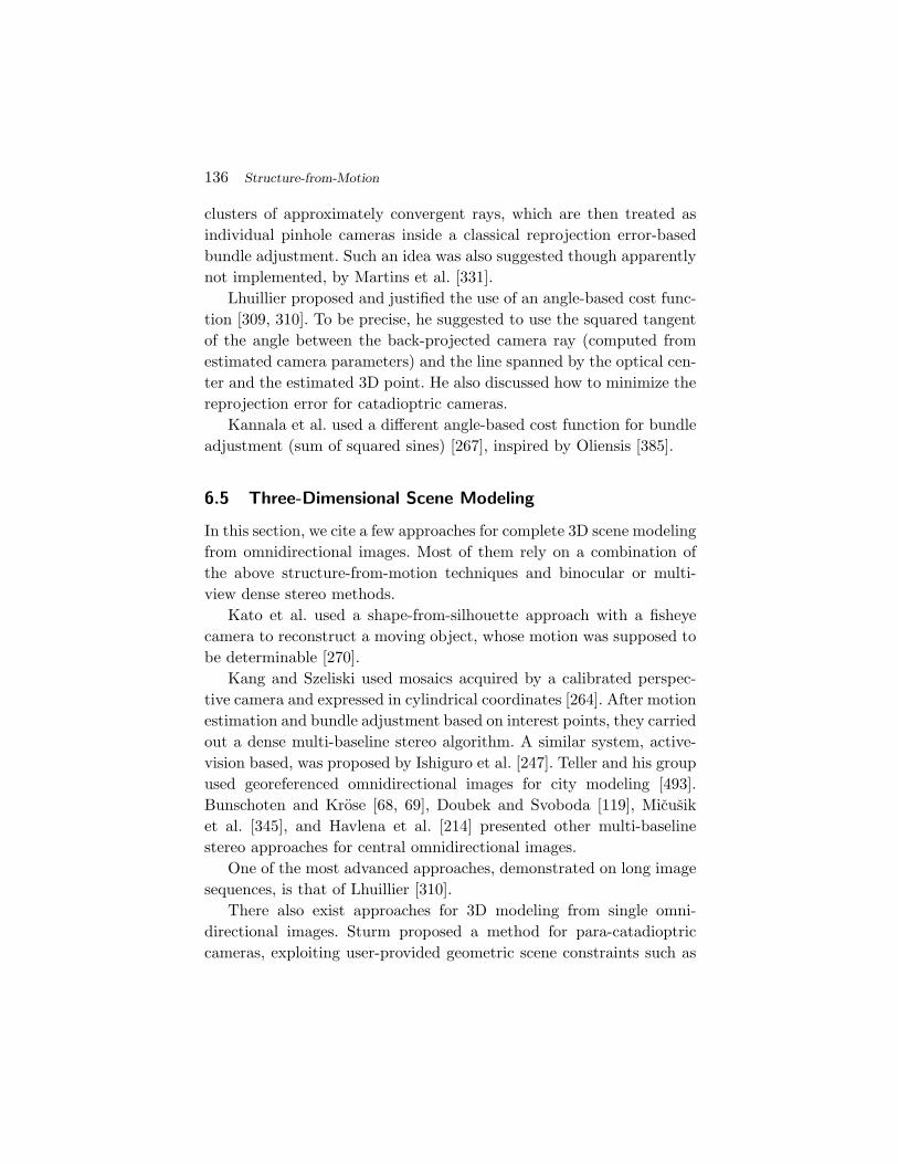
136 Structure-from-Motion

clusters of approximately convergent rays, which are then treated asindividual pinhole cameras inside a classical reprojection error-basedbundle adjustment. Such an idea was also suggested though apparentlynot implemented, by Martins et al. [331].

Lhuillier proposed and justified the use of an angle-based cost func-tion [309, 310]. To be precise, he suggested to use the squared tangentof the angle between the back-projected camera ray (computed fromestimated camera parameters) and the line spanned by the optical cen-ter and the estimated 3D point. He also discussed how to minimize thereprojection error for catadioptric cameras.

Kannala et al. used a different angle-based cost function for bundleadjustment (sum of squared sines) [267], inspired by Oliensis [385].

6.5 Three-Dimensional Scene Modeling

In this section, we cite a few approaches for complete 3D scene modelingfrom omnidirectional images. Most of them rely on a combination ofthe above structure-from-motion techniques and binocular or multi-view dense stereo methods.

Kato et al. used a shape-from-silhouette approach with a fisheyecamera to reconstruct a moving object, whose motion was supposed tobe determinable [270].

Kang and Szeliski used mosaics acquired by a calibrated perspec-tive camera and expressed in cylindrical coordinates [264]. After motionestimation and bundle adjustment based on interest points, they carriedout a dense multi-baseline stereo algorithm. A similar system, active-vision based, was proposed by Ishiguro et al. [247]. Teller and his groupused georeferenced omnidirectional images for city modeling [493].Bunschoten and Krose [68, 69], Doubek and Svoboda [119], Micusiket al. [345], and Havlena et al. [214] presented other multi-baselinestereo approaches for central omnidirectional images.

One of the most advanced approaches, demonstrated on long imagesequences, is that of Lhuillier [310].

There also exist approaches for 3D modeling from single omni-directional images. Sturm proposed a method for para-catadioptriccameras, exploiting user-provided geometric scene constraints such as

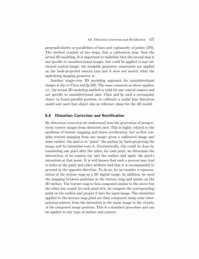
6.6 Distortion Correction and Rectification 137

perpendicularity or parallelism of lines and coplanarity of points [470].The method consists of two steps, first a calibration step, then theactual 3D modeling. It is important to underline that the second step isnot specific to omnidirectional images, but could be applied to any cal-ibrated central image: the available geometric constraints are appliedon the back-projected camera rays and it does not matter what theunderlying imaging geometry is.

Another single-view 3D modeling approach for omnidirectionalimages is due to Chen and Ip [93]. The same comment as above applies,i.e., the actual 3D modeling method is valid for any central camera andnot specific to omnidirectional ones. Chen and Ip used a rectangularobject in fronto-parallel position, to calibrate a radial lens distortionmodel and used that object also as reference plane for the 3D model.

6.6 Distortion Correction and Rectification

By distortion correction we understand here the generation of perspec-tively correct images from distorted ones. This is highly related to theproblems of texture mapping and stereo rectification. Let us first con-sider texture mapping from one image: given a calibrated image andsome surface, the goal is to “paint” the surface by back-projecting theimage and its intensities onto it. Geometrically, this could be done byconsidering one pixel after the other; for each pixel, we determine theintersection of its camera ray and the surface and apply the pixel’sintensities at that point. It is well known that such a process may leadto holes in the paint and other artifacts and that it is recommended toproceed in the opposite direction. To do so, let us consider a represen-tation of the texture map as a 2D digital image. In addition, we needthe mapping between positions in the texture map and points on the3D surface. The texture map is then computed similar to the above butthe other way round: for each pixel of it, we compute the correspondingpoint on the surface and project it into the input image. The intensitiesapplied to the texture map pixel are then computed using some inter-polation scheme, from the intensities in the input image in the vicinityof the computed image position. This is a standard procedure and canbe applied to any type of surface and camera.

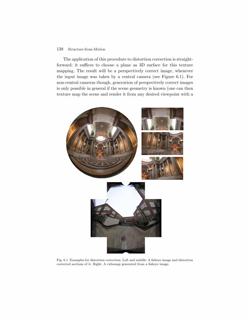
138 Structure-from-Motion

The application of this procedure to distortion correction is straight-forward: it suffices to choose a plane as 3D surface for this texturemapping. The result will be a perspectively correct image, wheneverthe input image was taken by a central camera (see Figure 6.1). Fornon-central cameras though, generation of perspectively correct imagesis only possible in general if the scene geometry is known (one can thentexture map the scene and render it from any desired viewpoint with a

Fig. 6.1 Examples for distortion correction. Left and middle: A fisheye image and distortioncorrected sections of it. Right: A cubemap generated from a fisheye image.

6.6 Distortion Correction and Rectification 139

virtual perspective camera). Swaminathan et al. proposed an approachto obtain good approximations of perspective views if the scene struc-ture is unknown but if simple priors on it are available [483]. A similarapproach, for misaligned hyper-catadioptric cameras, was proposed byJeng and Tsai [256]. Ding and Yu proposed an interactive approach forminimizing distortions in multi-perspective images that can be modeledusing the general linear camera model (GLC, see Section 3.4.4) [116].This problem is an instance of the more general image-based renderingproblem [181, 307].

As a sidenote, let us mention an optical procedure for generatingperspective images from a fisheye image, explained and demonstratedin 1925 by Beck [48]: he placed the negative of the fisheye image in thecamera and reversed the action of the latter, by illuminating the neg-ative and placing a photoplate in front of the camera. The photoplatethen gets imprinted with a perspective photograph corresponding tothe part of the fisheye’s field of view covered by the plate.

Using planar 3D surfaces for distortion correction has its limits,since a hemispheric field of view would require an infinitely large texturemap to hold the entire distortion-corrected input image. An alternativeis to use cubemaps, i.e., where partial perspective view are renderedonto the insides of a virtual cube, see Figure 6.1 and for example thepaper [265] by Kangni and Laganiere. Cubemaps and other useful pro-jections for environment mapping were well explained by Greene [187].See also the work [564] by Zelnik-Manor et al. for various other sugges-tions for projections used to warp spherical images to flat ones.

The above texture mapping scheme can be applied for other tasksthan the correction of non-perspective distortions. A typical exampleis to warp the usual circular omnidirectional images, which are hardto interpret by humans, into panoramic images; in that case, the 3Dsurface is the inside of a cylinder and the texture map corresponds tothe unrolled cylinder. Besides this, the generation of the texture mapis done exactly the same way as above.

Another application is stereo rectification. This consists in warpingan image pair such that the warped images have an epipolar geome-try where epipolar curves correspond to scanlines, i.e., where they arestraight lines and such that in addition corresponding epipolar lines

140 Structure-from-Motion

have the same vertical image coordinate. This enables efficient imple-mentations of stereo matching algorithms. As for perspective images,rectification can be achieved by applying appropriate homographies toeach image (there exist infinitely many solutions for these homogra-phies; different methods differ in the choice of a particular solution),see for example [21, 65, 176, 212, 325, 451].

Geyer and Daniilidis proposed a stereo rectification method forpara-catadioptric cameras, which applies conformal warping transfor-mations [169]. Banno and Kanade showed a rectification method forspherical images [24]. Heller and Pajdla proposed a stereographic rec-tification procedure for omnidirectional stereo pairs [217]. Instead ofmapping epipolar curves to scanlines, they suggested to map them tocircles; this is based on the observation that this way of rectifying min-imizes, in some sense, the distortions between original and rectifiedimages.

In 3D, one may picture stereo rectification as follows. Rectifiedimages correspond to perspective cameras which are oriented identically(i.e., their optical axes are parallel and the image planes are rotatedthe same way) have the same focal length and whose baseline is par-allel to the horizontal image direction. Given an input stereo pair, onemay transform it into a rectified geometry, as follows. First, computethe baseline and choose any planar surface that is parallel to the base-line, at some finite distance from it. That surface will play the role ofimage plane for the rectified images. Next, for each camera, computethe rotation that would make the optical axis orthogonal to that planeand such that the image plane’s horizontal axis becomes parallel to thebaseline. Finally, one has to zoom in or out one or both of the viewsby appropriate factors that lead to equal focal lengths for both images.Rotating a camera in 3D and changing its focal length is equivalent toapplying an appropriate projective transformation on its 2D image, thehomography used in rectification algorithms.

This principle can be applied to any central camera, even non-perspective ones. The warping transformations are no longer homo-graphies in general but this does not matter; all that is needed is theforward projection for the cameras, the determination of the rectified

6.6 Distortion Correction and Rectification 141

image plane, and the application of the above distortion correctionmethod.

One problem with this approach is that a planar image surface is notadequate for handling wide field of view cameras, as explained above.A second main problem is that the case where an epipole lies insidethe image cannot be handled; it would again require an infinitely largerectified image.

For a fully general solution, one thus has to use other projectionsurfaces than planes. Roy et al. used a cylindrical surface, whose axis isorthogonal to the baseline [431]. The final rectified images are obtainedby projecting the input images on the cylinder and unrolling it. If aparametric projection model is available for both cameras, then themapping from rectified to original images can be written in closed form.

Fig. 6.2 Example of the rectification procedure of Pollefeys et al. On the left, two inputimages (the epipoles are marked as white dots), on the right the two rectified images.Courtesy of Marc Pollefeys [404].

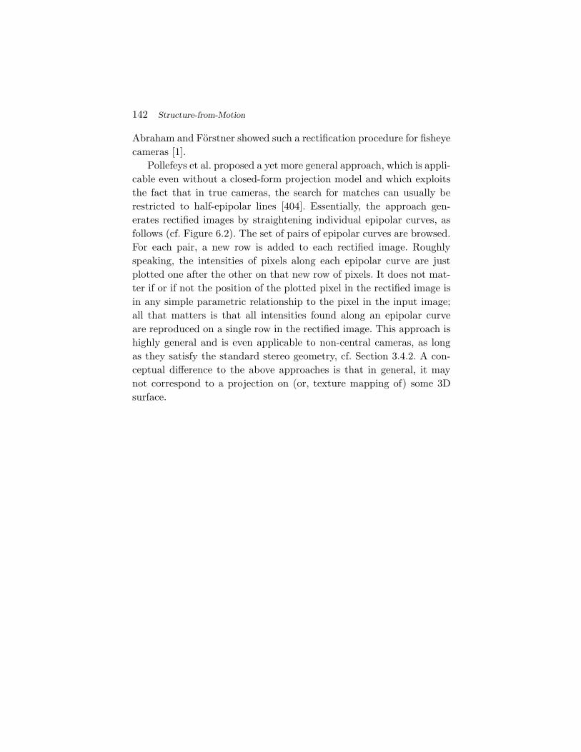
142 Structure-from-Motion

Abraham and Forstner showed such a rectification procedure for fisheyecameras [1].

Pollefeys et al. proposed a yet more general approach, which is appli-cable even without a closed-form projection model and which exploitsthe fact that in true cameras, the search for matches can usually berestricted to half-epipolar lines [404]. Essentially, the approach gen-erates rectified images by straightening individual epipolar curves, asfollows (cf. Figure 6.2). The set of pairs of epipolar curves are browsed.For each pair, a new row is added to each rectified image. Roughlyspeaking, the intensities of pixels along each epipolar curve are justplotted one after the other on that new row of pixels. It does not mat-ter if or if not the position of the plotted pixel in the rectified image isin any simple parametric relationship to the pixel in the input image;all that matters is that all intensities found along an epipolar curveare reproduced on a single row in the rectified image. This approach ishighly general and is even applicable to non-central cameras, as longas they satisfy the standard stereo geometry, cf. Section 3.4.2. A con-ceptual difference to the above approaches is that in general, it maynot correspond to a projection on (or, texture mapping of) some 3Dsurface.

7Concluding Remarks

We have described some image acquisition technologies and associatedcamera models, with an emphasis on omnidirectional cameras. Princi-ples and existing works on basic issues for geometric computer vision,such as epipolar geometry, calibration, and structure-from-motion, werereviewed. One of the goals in writing this monograph was to give a sur-vey of the literature and to highlight links between existing works andunderlying principles. While aiming at a certain level of exhaustivenessin the coverage of the literature, such a survey can never be complete;we apologize for any significant omission. The reader is invited to notifythe authors of works that should be cited; an addendum to this mono-graph shall be maintained on the first author’s website.

Let us briefly summarize what we consider some of the mainissues we were trying to convey. We concentrated on models for back-projection, in order to stress that these enable a simple and system-atic formulation of epipolar geometry, self-calibration, pose and motionestimation, and the projection of 3D lines. For distortion correctionand bundle adjustment however, forward projection should ideally beused. An important issue we discussed concerns the choice of cameramodel, for example if or if not a non-central model is appropriate in

143

144 Concluding Remarks

some application. Our conclusion is that there is no single and simpleanswer, but that this choice depends on multiple factors such as the“true” camera geometry, the amount of noise in data, the distributionof calibration points, and so forth.

Finally, we note that this monograph is restricted to geometricaspects of omnidirectional vision. Equally if not more important, areoptical and photometric characteristics; these are well explained andstudied for example by Okatani and Deguchi [384] and in various papersby Nayar et al.

Acknowledgments

P. Sturm is grateful to the Alexander-von-Humboldt Foundation for aResearch Fellowship supporting his sabbatical at TU Munich, duringwhich the largest part of this manuscript was written. He also acknowl-edges support by the French ANR project CAVIAR which supportedpart of the research carried out that eventually lead to the idea of writ-ing this monograph. J. Barreto and P. Sturm are thankful for their sup-port by the French-Portuguese collaboration program PHC Pessoa. Theauthors wish to thank Tomas Pajdla for comments on the manuscriptand Aseem Agarwala, Frederic Devernay, Sujit Kuthirummal, MarcPollefeys, Ryusuke Sagawa, and Steve Seitz for kindly allowing us touse images of their work.

145

References

[1] S. Abraham and W. Forstner, “Fish-eye-stereo calibration and epipolar rec-tification,” ISPRS Journal of Photogrammetry and Remote Sensing, vol. 59,no. 5, pp. 278–288, 2005.

[2] E. Adelson and J. Wang, “Single lens stereo with a plenoptic camera,”IEEE Transactions on Pattern Analysis and Machine Intelligence, vol. 14,pp. 99–106, February 1992.

[3] G. Adorni, M. Mordonini, S. Cagnoni, and A. Sgorbissa, “Omnidirectionalstereo systems for robot navigation,” in Proceedings of the Workshop on Omni-directional Vision and Camera Networks, Madison, Wisconsin, USA, 2003.

[4] A. Agarwala, M. Agrawala, M. Cohen, D. Salesin, and R. Szeliski, “Pho-tographing long scenes with multi-viewpoint panoramas,” in Proceedings ofSIGGRAPH, Boston, USA, pp. 853–861, 2006.

[5] A. Agrawal, Y. Taguchi, and S. Ramalingam, “Analytical forward projec-tion for axial non-central dioptric & catadioptric cameras,” in Proceedingsof the 11th European Conference on Computer Vision, Heraklion, Greece,pp. 129–143, 2010.

[6] M. Agrawal and L. Davis, “Camera calibration using spheres: A semi-definiteprogramming approach,” in Proceedings of the 9th IEEE International Con-ference on Computer Vision, Nice, France, pp. 782–791, 2003.

[7] M. Ahmed and A. Farag, “A neural approach to zoom-lens camera calibrationfrom data with outliers,” Image and Vision Computing, vol. 20, no. 9–10,pp. 619–630, 2002.

[8] M. Ahmed and A. Farag, “Nonmetric calibration of camera lens distortion:Differential methods and robust estimation,” IEEE Transactions on ImageProcessing, vol. 14, pp. 1215–1230, August 2005.

146

References 147

[9] M. Ahmed, E. Hemayed, and A. Farag, “Neurocalibration: A neural networkthat can tell camera calibration parameters,” in Proceedings of the 7th IEEEInternational Conference on Computer Vision, Kerkyra, Greece, pp. 463–468,1999.

[10] O. Ait-Aider, N. Andreff, J.-M. Lavest, and P. Martinet, “Simultaneous objectpose and velocity computation using a single view from a rolling shutter cam-era,” in Proceedings of the 9th European Conference on Computer Vision,Graz, Austria, (H. Bischof and A. Leonardis, eds.), pp. 56–68, Springer-Verlag,2006.

[11] S. Al-Ajlouni and C. Fraser, “Zoom-dependent calibration for consumer grade-cameras,” in Proceedings of the ISPRS Commission V Symposium on ImageEngineering and Vision Metrology, Dresden, Germany, pp. 20–25, September2006.

[12] D. Aliaga, “Accurate catadioptric calibration for real-time pose estimation inroom-size environments,” in Proceedings of the 8th IEEE International Con-ference on Computer Vision, Vancouver, Canada, pp. 127–134, 2001.

[13] J. Aloimonos, “Perspective approximations,” Image and Vision Computing,vol. 8, pp. 179–192, August 1990.

[14] L. Alvarez, L. Gomez, and J. Sendra, “An algebraic approach to lens distortionby line rectification,” Journal of Mathematical Imaging and Vision, vol. 35,pp. 36–50, September 2009.

[15] J. Arnspang, H. Nielsen, M. Christensen, and K. Henriksen, “Using mirrorcameras for estimating depth,” in Proceedings of the 6th International Confer-ence on Computer Analysis of Images and Patterns, Prague, Czech Republic,pp. 711–716, 1995.

[16] N. Asada, A. Amano, and M. Baba, “Photometric calibration of zoom lenssystems,” in Proceedings of the 13th International Conference on PatternRecognition, Vienna, Austria, pp. 186–190, IEEE Computer Society Press,August 1996.

[17] K. Asari, S. Kumar, and D. Radhakrishnan, “A new approach for nonlin-ear distortion correction in endoscopic images based on least squares estima-tion,” IEEE Transactions on Medical Imaging, vol. 18, pp. 345–354, April1999.

[18] C. Aschenbrenner, “Neue Gerate und Methoden fur die photogrammetrischeErschließung unerforschter Gebiete,” Bildmessung und Luftbildwesen, vol. 4,no. 1, pp. 30–38, 1929.

[19] K. Atkinson, ed., Close Range Photogrammetry and Machine Vision. WhittlesPublishing, 1996.

[20] O. Avni, T. Baum, G. Katzir, and E. Rivlin, “Recovery of 3D animal motionsusing cameras and mirrors,” Machine Vision and Applications, vol. 21, no. 6,pp. 879–888, 2010.

[21] N. Ayache, Stereovision and Sensor Fusion. Cambridge, MA, USA: The MITPress, 1990.

[22] S. Baker and S. Nayar, “A theory of single-viewpoint catadioptric image for-mation,” International Journal of Computer Vision, vol. 35, no. 2, pp. 1–22,1999.

148 References

[23] H. Bakstein and T. Pajdla, “Panoramic mosaicing with a 180◦ field of viewlens,” in Proceedings of the Workshop on Omnidirectional Vision, Copenhagen,Denmark, pp. 60–68, 2002.

[24] A. Banno and K. Ikeuchi, “Omnidirectional texturing based on robust 3D reg-istration through Euclidean reconstruction from two spherical images,” Com-puter Vision and Image Understanding, vol. 114, no. 4, pp. 491–499, 2010.

[25] J. Barreto, “General central projection systems: Modeling, calibration andvisual servoing,” PhD thesis, Department of Electrical and Computer Engi-neering, University of Coimbra, Portugal, September 2003.

[26] J. Barreto, “A unifying geometric representation for central projectionsystems,” Computer Vision and Image Understanding, vol. 103, no. 3,pp. 208–217, 2006.

[27] J. Barreto, “Unifying image plane liftings for central catadioptric and diop-tric cameras,” in Imaging Beyond the Pinhole Camera, (K. Daniilidis andR. Klette, eds.), Springer-Verlag, August 2006.

[28] J. Barreto and H. Araujo, “Issues on the geometry of central catadioptricimage formation,” in Proceedings of the IEEE Conference on Computer Visionand Pattern Recognition, Kauai, Hawaii, USA, pp. 422–427, 2001.

[29] J. Barreto and H. Araujo, “Geometric properties of central catadioptric lineimages,” in Proceedings of the 7th European Conference on Computer Vision,Copenhagen, Denmark, pp. 237–251, 2002.

[30] J. Barreto and H. Araujo, “Paracatadioptric camera calibration using lines,”in Proceedings of the 9th IEEE International Conference on Computer Vision,Nice, France, pp. 1359–1365, 2003.

[31] J. Barreto and H. Araujo, “Geometric properties of central catadioptric lineimages and their application in calibration,” IEEE Transactions on PatternAnalysis and Machine Intelligence, vol. 27, no. 8, pp. 1327–1333, 2005.

[32] J. Barreto and H. Araujo, “Fitting conics to paracatadioptric projectionsof lines,” Computer Vision and Image Understanding, vol. 103, no. 3,pp. 151–165, 2006.

[33] J. Barreto and K. Daniilidis, “Wide area multiple camera calibration and esti-mation of radial distortion,” in Proceedings of the 5th Workshop on Omnidirec-tional Vision, Camera Networks and Non-Classical Cameras, Prague, CzechRepublic, 2004.

[34] J. Barreto and K. Daniilidis, “Fundamental matrix for cameras with radial dis-tortion,” in Proceedings of the 10th IEEE International Conference on Com-puter Vision, Beijing, China, pp. 625–632, 2005.

[35] J. Barreto and K. Daniilidis, “Epipolar geometry of central projection systemsusing veronese maps,” in Proceedings of the IEEE Conference on ComputerVision and Pattern Recognition, New York, USA, pp. 1258–1265, 2006.

[36] J. Barreto, J. Roquette, P. Sturm, and F. Fonseca, “Automatic camera cal-ibration applied to medical endoscopy,” in Proceedings of the 20th BritishMachine Vision Conference, London, England, 2009.

[37] J. Barreto, R. Swaminathan, and J. Roquette, “Non parametric distortioncorrection in endoscopic medical images,” in Proceedings of 3DTV-CON Con-ference on The True Vision, Capture, Transmission and Display of 3D Video,Kos, Greece, 2007.

References 149

[38] M. Barth and C. Barrows, “A fast panoramic imaging system and intelli-gent imaging technique for mobile robots,” in Proceedings of the IEEE/RSJInternational Conference on Intelligent Robots and Systems, Osaka, Japan,pp. 626–633, 1996.

[39] O. Baschin, “Eine einfache Methode der stereophotogrammetrischenKustenvermessung,” Petermanns Mitteilungen, 1908.

[40] Y. Bastanlar, L. Puig, P. Sturm, J. Guerrero, and J. Barreto, “DLT-like cali-bration of central catadioptric cameras,” in Proceedings of the 8th Workshopon Omnidirectional Vision, Camera Networks and Non-Classical Cameras,Marseille, France, October 2008.

[41] A. Basu and S. Licardie, “Alternative models for fish-eye lenses,” PatternRecognition Letters, vol. 16, pp. 433–441, April 1995.

[42] J. Batista, H. Araujo, and A. de Almeida, “Iterative multi-step explicit cam-era calibration,” in Proceedings of the 6th IEEE International Conference onComputer Vision, Bombay, India, pp. 709–714, January 1998.

[43] G. Batog, X. Goaoc, and J. Ponce, “Admissible linear map models of linearcameras,” in Proceedings of the IEEE Conference on Computer Vision andPattern Recognition, San Francisco, USA, 2010.

[44] E. Bayro-Corrochano and C. Lopez-Franco, “Omnidirectional vision: Unifiedmodel using conformal geometry,” in Proceedings of the 8th European Confer-ence on Computer Vision, Prague, Czech Republic, pp. 536–548, 2004.

[45] J. Bazin, C. Demonceaux, P. Vasseur, and I. Kweon, “Motion estimation bydecoupling rotation and translation in catadioptric vision,” Computer Visionand Image Understanding, vol. 114, no. 2, pp. 254–273, 2010.

[46] S. Beauchemin and R. Bajcsy, “Modelling and removing radial and tangen-tial distortions in spherical lenses,” in Proceedings of the 10th InternationalWorkshop on Theoretical Foundations of Computer Vision, Dagstuhl Castle,Germany, (R. Klette, T. Huang, and G. Gimel’farb, eds.), pp. 1–21, Springer-Verlag, March 2000.

[47] S. Beauchemin, R. Bajcsy, and G. Givaty, “A unified procedure for calibratingintrinsic parameters of fish-eye lenses,” in Proceedings of Vision interface,Trois-Rivieres, Canada, pp. 272–279, 1999.

[48] C. Beck, “Apparatus to photograph the whole sky,” Journal of ScientificInstruments, vol. 2, no. 4, pp. 135–139, 1925.

[49] R. Benosman, E. Deforas, and J. Devars, “A new catadioptric sensor for thepanoramic vision of mobile robots,” in Proceedings of the IEEE Workshop onOmnidirectional Vision, Hilton Head Island, South Carolina, 2000.

[50] R. Benosman and S. Kang, “A brief historical perspective on panorama,”in Panoramic Vision: Sensors, Theory, and Applications, (R. Benosman andS. Kang, eds.), pp. 5–20, Springer-Verlag, 2001.

[51] R. Benosman and S. Kang, eds., Panoramic Vision. Springer-Verlag, 2001.[52] R. Benosman, T. Maniere, and J. Devars, “Multidirectional stereovision

sensor, calibration and scenes reconstruction,” in Proceedings of the 13th Inter-national Conference on Pattern Recognition, Vienna, Austria, pp. 161–165,1996.

[53] H. Beyer, “Accurate calibration of CCD cameras,” in Proceedings of the IEEEConference on Computer Vision and Pattern Recognition, Urbana-Champaign,Illinois, USA, pp. 96–101, 1992.

150 References

[54] S. Bogner, “An introduction to panospheric imaging,” in Proceedings of theIEEE International Conference on Systems, Man and Cybernetics, Vancouver,Canada, pp. 3099–3106, 1995.

[55] J. Boland, “Cameras and sensing systems,” in Manual of Photogrammetry,Fifth Edition, (C. McGlone, ed.), ch. 8, pp. 581–676, Falls Church, Virginia,USA: American Society of Photogrammetry and Remote Sensing, 2004.

[56] R. Bolles, H. Baker, and D. Marimont, “Epipolar-plane image analysis: Anapproach to determining structure from motion,” International Journal ofComputer Vision, vol. 1, pp. 7–55, 1987.

[57] R. Boutteau, X. Savatier, J.-Y. Ertaud, and B. Mazari, “An omnidirec-tional stereoscopic system for mobile robot navigation,” in Proceedings of theIEEE International Workshop on Robotic and Sensors Environment, Ottawa,Canada, pp. 138–143, 2008.

[58] A. Bouwers and J. van der Sande, “A new camera of extremely high luminosityand resolution based on the concentric optical mirror system,” in Proceedingsof the VII ISPRS-Congress, Washington, USA, pp. 246/1–246/3, 1952.

[59] P. Brand, R. Mohr, and P. Bobet, “Distorsions optiques: Correction dans unmodele projectif,” Technical Report 1933, LIFIA–IMAG–INRIA Rhone-Alpes,Grenoble, France, June 1993.

[60] P. Brand, R. Mohr, and P. Bobet, “Distorsion optique: Correction dans unmodele projectif,” in Actes du 9eme Congres AFCET de Reconnaissance desFormes et Intelligence Artificielle, Paris, France, pp. 87–98, Paris, January1994.

[61] E. Brassart, L. Delahoche, C. Cauchois, C. Drocourt, C. Pegard, andM. Mouaddib, “Experimental results got with the omnidirectional vision sen-sor: SYCLOP,” in Proceedings of the IEEE Workshop on OmnidirectionalVision, Hilton Head Island, South Carolina, pp. 145–152, 2000.

[62] C. Brauer-Burchardt and K. Voss, “A new algorithm to correct fish-eye andstrong wide-angle-lens-distortion from single images,” in Proceedings of theIEEE International Conference on Image Processing, Thessaloniki, Greece,pp. 225–228, 2001.

[63] D. Brown, “Decentering distortion of lenses,” Photogrammetric Engineering,vol. 32, pp. 444–462, May 1966.

[64] D. Brown, “Close-range camera calibration,” Photogrammetric Engineering,vol. 37, no. 8, pp. 855–866, 1971.

[65] L. Brown, “A survey of image registration techniques,” ACM Computing Sur-veys, vol. 24, pp. 325–376, December 1992.

[66] A. Bruckstein and T. Richardson, “Omniview cameras with curved surfacemirrors,” in Proceedings of the IEEE Workshop on Omnidirectional Vision,Hilton Head Island, South Carolina, pp. 79–84, 2000.

[67] T. Buchanan, “The twisted cubic and camera calibration,” Computer Vision,Graphics and Image Processing, vol. 42, pp. 130–132, April 1988.

[68] R. Bunschoten and B. Krose, “3D scene reconstruction from cylindricalpanoramic images,” Robotics and Autonomous Systems, vol. 41, no. 2–3,pp. 111–118, 2002.

[69] R. Bunschoten and B. Krose, “Robust scene reconstruction from an omni-directional vision system,” IEEE Transactions on Robotics and Automation,vol. 19, no. 2, pp. 351–357, 2002.

References 151

[70] A. Burner, “Zoom lens calibration for wind tunnel measurements,” in Proceed-ings of the SPIE Conference on Videometrics IV, Philadelphia, Pennsylvania,USA, (S. El-Hakim, ed.), pp. 19–33, SPIE — Society of Photo-Optical Instru-mentation Engineers, October 1995.

[71] P. Burns, “The history of the discovery of cinematography,” http://www.precinemahistory.net.

[72] M. Byrod, Z. Kukelova, K. Josephson, T. Pajdla, and K. Astrom, “Fast androbust numerical solutions to minimal problems for cameras with radial dis-tortion,” in Proceedings of the IEEE Conference on Computer Vision andPattern Recognition, Anchorage, USA, 2008.

[73] E. Cabral, J. de Souza Junior, and M. Hunold, “Omnidirectional stereo visionwith a hyperbolic double lobed mirror,” in Proceedings of the 15th Interna-tional Conference on Pattern Recognition, Cambridge, UK, pp. 1–4, 2004.

[74] C. Cafforio and F. Rocca, “Precise stereopsis with a single video camera,” inProceedings of the 3rd European Signal Processing Conference (EUSIPCO):Theories and Application, The Hague, Netherlands, pp. 641–644, 1986.

[75] V. Caglioti and S. Gasparini, “Localization of straight lines from single imagesusing off-axis catadioptric cameras,” in Proceedings of the 6th Workshop onOmnidirectional Vision, Camera Networks and Non-Classical Cameras, Bei-jing, China, 2005.

[76] V. Caglioti and S. Gasparini, “On the localization of straight lines in 3D spacefrom single 2D images,” in Proceedings of the IEEE Conference on ComputerVision and Pattern Recognition, San Diego, USA, pp. 1129–1134, 2005.

[77] V. Caglioti and S. Gasparini, ““How many planar viewing surfaces are there innoncentral catadioptric cameras?” Towards singe-image localization of spacelines,” in Proceedings of the IEEE Conference on Computer Vision and Pat-tern Recognition, New York, USA, pp. 1266–1273, 2006.

[78] V. Caglioti, P. Taddei, G. Boracchi, S. Gasparini, and A. Giusti, “Single-image calibration of off-axis catadioptric cameras using lines,” in Proceedingsof the 7th Workshop on Omnidirectional Vision, Camera Networks and Non-Classical Cameras, Rio de Janeiro, Brazil, 2007.

[79] S. Cagnoni, M. Mordonini, L. Mussi, and G. Adorni, “Hybrid stereo sensorwith omnidirectional vision capabilities: Overview and calibration proce-dures,” in Proceedings of the 14th International Conference on Image Analysisand Processing, Modena, Italy, pp. 99–104, 2007.

[80] Z. Cao, S. Oh, and E. Hall, “Dynamic omnidirectional vision for mobilerobots,” Journal of Robotic Systems, vol. 3, no. 1, pp. 5–17, 1986.

[81] B. Caprile and V. Torre, “Using vanishing points for camera calibration,”International Journal of Computer Vision, vol. 4, pp. 127–140, 1990.

[82] C. Cauchois, E. Brassart, L. Delahoche, and A. Clerentin, “3D localizationwith conical vision,” in Proceedings of the Workshop on OmnidirectionalVision and Camera Networks, Madison, Wisconsin, USA, 2003.

[83] C. Cauchois, E. Brassart, C. Drocourt, and P. Vasseur, “Calibration of theomnidirectional vision sensor: SYCLOP,” in Proceedings of the IEEE Inter-national Conference on Robotics and Automation, Detroit, Michigan, USA,pp. 1287–1292, May 1999.

152 References

[84] J. Chahl and M. Srinivasan, “Reflective surfaces for panoramic imaging,”Applied Optics, vol. 36, no. 31, pp. 8275–8285, 1997.

[85] G. Champleboux, S. Lavallee, P. Sautot, and P. Cinquin, “Accurate calibrationof cameras and range imaging sensors: The NPBS method,” in Proceedings ofthe IEEE International Conference on Robotics and Automation, Nice, France,pp. 1552–1558, May 1992.

[86] P. Chang and M. Hebert, “Omni-directional structure from motion,” in Pro-ceedings of the IEEE Workshop on Omnidirectional Vision, Hilton HeadIsland, South Carolina, pp. 127–133, 2000.

[87] A. Charriou and S. Valette, “Appareil photographique multiple pour etudessur la prise de vues aeriennes,” in Proceedings of the V ISPRS-Congress, Rome,Italy, pp. 154–157, 1938.

[88] C.-S. Chen and W.-Y. Chang, “On pose recovery for generalized visual sen-sors,” IEEE Transactions on Pattern Analysis and Machine Intelligence,vol. 26, pp. 848–861, July 2004.

[89] N.-Y. Chen, “Visually estimating workpiece pose in a robot hand using thefeature points method,” PhD thesis, University of Rhode Island, Kingston,1979.

[90] N.-Y. Chen, J. Birk, and R. Kelley, “Estimating workpiece pose using thefeature points method,” IEEE Transactions on Automatic Control, vol. 25,pp. 1027–1041, December 1980.

[91] Q. Chen, H. Wu, and T. Wada, “Camera calibration with two arbitrary copla-nar circles,” in Proceedings of the 8th European Conference on ComputerVision, Prague, Czech Republic, pp. 521–532, 2004.

[92] S. Chen, “Quicktime vr — an image-based approach to virtual environmentnavigation,” in Proceedings of SIGGRAPH, Los Angeles, USA, pp. 29–38,1995.

[93] Y. Chen and H. Ip, “Single view metrology of wide-angle lens images,” TheVisual Computer, vol. 22, no. 7, pp. 445–455, 2006.

[94] J. Clark and G. Follin, “A simple “equal area” calibration for fisheye photog-raphy,” Agricultural and Forest Meteorology, vol. 44, pp. 19–25, 1988.

[95] T. Clarke and J. Fryer, “The development of camera calibration methods andmodels,” Photogrammetric Record, vol. 91, no. 16, pp. 51–66, 1998.

[96] T. Clarke, X. Wang, and J. Fryer, “The principal point and CCD cameras,”Photogrammetric Record, vol. 92, no. 16, pp. 293–312, 1998.

[97] D. Claus and A. Fitzgibbon, “A plumbline constraint for the rational functionlens distortion model,” in Proceedings of the 16th British Machine VisionConference, Oxford, England, pp. 99–108, 2005.

[98] D. Claus and A. Fitzgibbon, “A rational function lens distortion model forgeneral cameras,” in Proceedings of the IEEE Conference on Computer Visionand Pattern Recognition, San Diego, USA, pp. 213–219, 2005.

[99] T. Conroy and J. Moore, “Resolution invariant surfaces for panoramicvision systems,” in Proceedings of the 7th IEEE International Conference onComputer Vision, Kerkyra, Greece, pp. 392–397, 1999.

[100] K. Cornelis, M. Pollefeys, and L. van Gool, “Lens distortion recoveryfor accurate sequential structure and motion recovery,” in Proceedings of

References 153

the 7th European Conference on Computer Vision, Copenhagen, Denmark,pp. 186–200, 2002.

[101] N. Cornille, “Accurate 3D shape and displacement measurement using a scan-ning electron microscope,” PhD thesis, University of South Carolina and Insti-tut National des Sciences Appliquees de Toulouse, June 2005.

[102] J. Crowley, P. Bobet, and C. Schmid, “Maintaining stereo calibration by track-ing image points,” in Proceedings of the IEEE Conference on Computer Visionand Pattern Recognition, New York, USA, pp. 483–488, June 1993.

[103] K. Daniilidis, “The page of omnidirectional vision,” http://www.cis.upenn.edu/∼kostas/omni.html.

[104] N. Daucher, M. Dhome, and J.-T. Lapreste, “Camera calibration from sphereimages,” in Proceedings of the 3rd European Conference on Computer Vision,Stockholm, Sweden, pp. 449–454, 1994.

[105] A. Davidhazy, “Camera for conical peripheral and panoramic photography,”SIGGRAPH Course, 2007.

[106] C. Davis and T.-H. Ho, “Using geometrical constraints for fisheye cameracalibration,” in Proceedings of the 6th Workshop on Omnidirectional Vision,Camera Networks and Non-Classical Cameras, Beijing, China, 2005.

[107] A. Davison, I. Reid, N. Molton, and O. Stasse, “MonoSLAM: Real-time singlecamera SLAM,” IEEE Transactions on Pattern Analysis and Machine Intel-ligence, vol. 29, no. 6, pp. 1052–1067, 2007.

[108] T. Debaecker, R. Benosman, and S. Ieng, “Cone-pixels camera models,” inProceedings of the 8th Workshop on Omnidirectional Vision, Camera Networksand Non-Classical Cameras, Marseille, France, 2008.

[109] C. Delherm, J.-M. Lavest, M. Dhome, and J.-T. Lapreste, “Dense reconstruc-tion by zooming,” in Proceedings of the 4th European Conference on ComputerVision, Cambridge, England, (B. Buxton and R. Cipolla, eds.), pp. 427–438,Springer-Verlag, 1996.

[110] X.-M. Deng, F.-C. Wu, and Y.-H. Wu, “An easy calibration method for centralcatadioptric cameras,” Acta Automatica Sinica, vol. 33, no. 8, pp. 801–808,2007.

[111] S. Derrien and K. Konolige, “Approximating a single viewpoint in panoramicimaging devices,” in Proceedings of the IEEE International Conference onRobotics and Automation, pp. 3931–3938, 2000.

[112] R. Descartes, Discours de la methode pour bien conduire sa raison, et chercherla verite dans les sciences. Ian Maire, Leyden, 1637.

[113] F. Devernay and O. Faugeras, “Straight lines have to be straight,” MachineVision and Applications, vol. 13, pp. 14–24, August 2001.

[114] M. Dhome, J. Lapreste, G. Rives, and M. Richetin, “Spatial localization ofmodelled objects of revolution in monocular perspective vision,” in Proceed-ings of the 1st European Conference on Computer Vision, Antibes, France,pp. 475–488, 1990.

[115] H. Dietz, “Fisheye digital imaging for under twenty dollars,” Technical Report,University of Kentucky, April 2006.

[116] Y. Ding and J. Yu, “Multiperspective distortion correction usingcollineations,” in Proceedings of the Asian Conference on Computer Vision,Tokyo, Japan, pp. 95–105, 2007.

154 References

[117] E. Dolezal, “Photogrammetrische Losung des Wolkenproblems aus einemStandpunkt unter Verwendung der Reflexe,” Sitzungsberichte KaiserlicheAkademie der Wissenschaften, mathematisch-naturwissenschaftliche Klasse,Abteilung IIa, vol. 111, pp. 788–813, 1902.

[118] F. Dornaika and J. Elder, “Image registration for foveated omnidirectionalsensing,” in Proceedings of the 7th European Conference on Computer Vision,Copenhagen, Denmark, pp. 606–620, 2002.

[119] P. Doubek and T. Svoboda, “Reliable 3D reconstruction from a few cata-dioptric images,” in Proceedings of the Workshop on Omnidirectional Vision,Copenhagen, Denmark, 2002.

[120] J. Drareni, P. Sturm, and S. Roy, “Plane-based calibration for linear cameras,”in Proceedings of the 8th Workshop on Omnidirectional Vision, Camera Net-works and Non-Classical Cameras, Marseille, France, October 2008.

[121] D. Drucker and P. Locke, “A natural classiffication of curves and surfaceswith reflection properties,” Mathematics Magazine, vol. 69, no. 4, pp. 249–256, 1996.

[122] F. Du and M. Brady, “Self-calibration of the intrinsic parameters of camerasfor active vision systems,” in Proceedings of the IEEE Conference on Com-puter Vision and Pattern Recognition, New York, USA, pp. 477–482, IEEEComputer Society Press, 1993.

[123] A. Dunne, J. Mallon, and P. Whelan, “A comparison of new generic cameracalibration with the standard parametric approach,” in Proceedings of IAPRConference on Machine Vision Applications, Tokyo, Japan, pp. 114–117, 2007.

[124] A. Dunne, J. Mallon, and P. Whelan, “Efficient generic calibration method forgeneral cameras with single centre of projection,” in Proceedings of the 11thIEEE International Conference on Computer Vision, Rio de Janeiro, Brazil,2007.

[125] A. Dunne, J. Mallon, and P. Whelan, “Efficient generic calibration methodfor general cameras with single centre of projection,” Computer Vision andImage Understanding, vol. 114, no. 2, pp. 220–233, 2010.

[126] T. Echigo, “A camera calibration technique using three sets of parallel lines,”Machine Vision and Applications, vol. 3, no. 3, pp. 159–167, 1990.

[127] M. El-Melegy and A. Farag, “Nonmetric lens distortion calibration: Closed-form solutions, robust estimation and model selection,” in Proceedings ofthe 9th IEEE International Conference on Computer Vision, Nice, France,pp. 554–559, 2003.

[128] R. Enciso, T. Vieville, and A. Zisserman, “An affine solution to euclideancalibration for a zoom lens,” in Proceedings of the ALCATECH Workshop,Denmark, pp. 21–27, July 1996.

[129] C. Engels, H. Stewenius, and D. Nister, “Bundle adjustment rules,” in Pro-ceedings of ISPRS Symposium on Photogrammetric Computer Vision, Bonn,Germany, 2006.

[130] F. Espuny, “A closed-form solution for the generic self-calibration of cen-tral cameras from two rotational flows,” in Proceedings of the InternationalConference on Computer Vision Theory and Applications, Barcelona, Spain,pp. 26–31, 2007.

References 155

[131] F. Espuny and J. Burgos Gil, “Generic self-calibration of central camerasfrom two “real” rotational flows,” in Proceedings of the 8th Workshop onOmnidirectional Vision, Camera Networks and Non-Classical Cameras, Mar-seille, France, 2008.

[132] J. Fabrizio and J. Devars, “An analytical solution to the perspective-n-pointproblem for common planar camera and for catadioptric sensor,” InternationalJournal of Image and Graphics, vol. 8, pp. 135–155, January 2008.

[133] J. Fabrizio, J. Tarel, and R. Benosman, “Calibration of panoramic catadiop-tric sensors made easier,” in Proceedings of the Workshop on OmnidirectionalVision, Copenhagen, Denmark, pp. 45–52, 2002.

[134] W. Faig, “Calibration of close-range photogrammetric systems: Mathemati-cal formulation,” Photogrammetric Engineering & Remote Sensing, vol. 41,pp. 1479–1486, December 1975.

[135] H. Farid and A. Popescu, “Blind removal of image non-linearities,” in Pro-ceedings of the 8th IEEE International Conference on Computer Vision, Van-couver, Canada, pp. 76–81, 2001.

[136] O. Fassig, “A revolving cloud camera,” Monthly Weather Review, vol. 43, no. 6,pp. 274–275, 1915.

[137] O. Faugeras, Q.-T. Luong, and T. Papadopoulo, The Geometry of MultipleImages. MIT Press, March 2001.

[138] O. Faugeras and B. Mourrain, “On the geometry and algebra of the point andline correspondences between n images,” in Proceedings of the 5th IEEE Inter-national Conference on Computer Vision, Cambridge, Massachusetts, USA,pp. 951–956, June 1995.

[139] D. Feldman, T. Pajdla, and D. Weinshall, “On the epipolar geometry of thecrossed-slits projection,” in Proceedings of the 9th IEEE International Con-ference on Computer Vision, Nice, France, pp. 988–995, 2003.

[140] R. Fergus, A. Torralba, and W. Freeman, “Random lens imaging,” MIT-CSAIL-TR-2006-058, Massachusetts Institute of Technology, September 2006.

[141] C. Fermuller and Y. Aloimonos, “Geometry of eye design: Biology andtechnology,” in Proceedings of the 10th International Workshop on Theoret-ical Foundations of Computer Vision, Dagstuhl Castle, Germany, pp. 22–38,Springer-Verlag, 2001.

[142] R. Feynman, R. Leighton, and M. Sands, The Feynman Lectures on Physics,Vol. 1, Mainly Mechanics, Radiation, and Heat. Addison-Wesley, 1963.

[143] M. Fiala and A. Basu, “Feature extraction and calibration for stereo recon-struction using non-svp optics in a panoramic stereo-vision sensor,” in Pro-ceedings of the Workshop on Omnidirectional Vision, Copenhagen, Denmark,2002.

[144] S. Finsterwalder, “Die geometrischen Grundlagen der Photogrammetrie,”Jahresbericht Deutscher Mathematik, vol. 6, pp. 1–44, 1899.

[145] A. Fitzgibbon, “Simultaneous linear estimation of multiple view geometry andlens distortion,” in Proceedings of the IEEE Conference on Computer Visionand Pattern Recognition, Kauai, Hawaii, USA, pp. 125–132, 2001.

[146] M. Fleck, “Perspective projection: The wrong imaging model,” TechnicalReport TR 95–01, Department of Computer Science, University of Iowa, IowaCity, IA 52242, USA, 1995.

156 References

[147] W. Forstner, B. Wrobel, F. Paderes, R. Craig, C. Fraser, and J. Dolloff, “Ana-lytical photogrammetric operations,” in Manual of Photogrammetry, FifthEdition, (C. McGlone, ed.), ch. 11, pp. 763–948, Falls Church, Virginia, USA:American Society of Photogrammetry and Remote Sensing, 2004.

[148] O. Frank, R. Katz, C. Tisse, and H. Durrant-Whyte, “Camera calibration forminiature, low-cost, wide-angle imaging system,” in Proceedings of the 18thBritish Machine Vision Conference, Warwick, England, 2007.

[149] C. Fraser, “Digital camera self-calibration,” ISPRS Journal of Photogramme-try and Remote Sensing, vol. 52, no. 4, pp. 149–159, 1997.

[150] C. Fraser and S. Al-Ajlouni, “Zoom-dependent calibration for consumer grade-cameras,” Photogrammetric Engineering & Remote Sensing, vol. 72, pp. 1017–1026, September 2006.

[151] L. Fritz and H. Schmid, “Stellar calibration of the orbigon lens,” Photogram-metric Engineering, vol. 40, no. 1, pp. 101–115, 1974.

[152] J. Fryer and D. Brown, “Lens distortion for close-range photogrammetry,”Photogrammetric Engineering & Remote Sensing, vol. 52, pp. 51–58, January1986.

[153] S. Gachter, T. Pajdla, and B. Micusık, “Mirror design for an omnidirectionalcamera with a space variant imager,” in Proceedings of the Workshop on Omni-directional Vision Applied to Robotic Orientation and Nondestructive Testing,Budapest, Hungary, 2001.

[154] C. Gao and N. Ahuja, “Single camera stereo using planar parallel plate,”in Proceedings of the 15th International Conference on Pattern Recognition,Cambridge, UK, pp. 108–111, 2004.

[155] C. Gao, H. Hua, and N. Ahuja, “A hemispherical imaging camera,” ComputerVision and Image Understanding, vol. 114, no. 2, pp. 168–178, 2010.

[156] J. Gaspar, “Omnidirectional vision for mobile robot navigation,” PhD thesis,Universidade Tecnica de Lisboa, Portgual, December 2002.

[157] J. Gaspar, C. Decco, J. Okamoto Jr, and J. Santos-Victor, “Constant resolu-tion omnidirectional cameras,” in Proceedings of the Workshop on Omnidirec-tional Vision, Copenhagen, Denmark, pp. 27–34, 2002.

[158] S. Gasparini and P. Sturm, “Multi-view matching tensors from lines for gen-eral camera models,” in Tensors in Image Processing and Computer Vision,(S. Aja-Fernandez, R. de Luis Garcıa, D. Tao, and X. Li, eds.), Springer-Verlag, 2009.

[159] S. Gasparini, P. Sturm, and J. Barreto, “Plane-based calibration of centralcatadioptric cameras,” in Proceedings of the 12th IEEE International Confer-ence on Computer Vision, Kyoto, Japan, 2009.

[160] M. Gasser, “Mehrfachkammer fur Aufnahmen aus Luftfahrzeugen,” PatentNo. 469,413, Reichspatentamt, Germany, 1926.

[161] D. Gennery, “Generalized camera calibration including fish-eye lenses,” Inter-national Journal of Computer Vision, vol. 68, pp. 239–266, July 2006.

[162] T. Georgiev, C. Intwala, and D. Babacan, “Light-field capture by multiplexingin the frequency domain,” Technical Report, Adobe Systems Incorporated,April 2007.

References 157

[163] C. Geyer and K. Daniilidis, “Catadioptric camera calibration,” in Proceed-ings of the 7th IEEE International Conference on Computer Vision, Kerkyra,Greece, pp. 398–404, 1999.

[164] C. Geyer and K. Daniilidis, “A unifying theory of central panoramic systemsand practical applications,” in Proceedings of the 6th European Conference onComputer Vision, Dublin, Ireland, (D. Vernon, ed.), pp. 445–461, Springer-Verlag, June 2000.

[165] C. Geyer and K. Daniilidis, “Catadioptric projective geometry,” InternationalJournal of Computer Vision, vol. 45, no. 3, pp. 223–243, 2001.

[166] C. Geyer and K. Daniilidis, “Structure and motion from uncalibrated cata-dioptric views,” in Proceedings of the IEEE Conference on Computer Visionand Pattern Recognition, Kauai, Hawaii, USA, pp. 279–286, 2001.

[167] C. Geyer and K. Daniilidis, “Paracatadioptric camera calibration,” IEEETransactions on Pattern Analysis and Machine Intelligence, vol. 24,pp. 687–695, May 2002.

[168] C. Geyer and K. Daniilidis, “Properties of the catadioptric fundamentalmatrix,” in Proceedings of the 7th European Conference on Computer Vision,Copenhagen, Denmark, (A. Heyden, G. Sparr, M. Nielsen, and P. Johansen,eds.), pp. 140–154, 2002.

[169] C. Geyer and K. Daniilidis, “Conformal rectification of an omnidirectionalstereo pair,” in Proceedings of the Workshop on Omnidirectional Vision andCamera Networks, Madison, Wisconsin, USA, 2003.

[170] C. Geyer and K. Daniilidis, “Mirrors in motion: Epipolar geometry and motionestimation,” in Proceedings of the 9th IEEE International Conference on Com-puter Vision, Nice, France, pp. 766–773, 2003.

[171] C. Geyer, M. Meingast, and S. Sastry, “Geometric models of rolling-shuttercameras,” in Proceedings of the 6th Workshop on Omnidirectional Vision,Camera Networks and Non-Classical Cameras, Beijing, China, 2005.

[172] C. Geyer and H. Stewenius, “A nine-point algorithm for estimating para-catadioptric fundamental matrices,” in Proceedings of the 11th IEEE Inter-national Conference on Computer Vision, Rio de Janeiro, Brazil, pp. 1–8,2007.

[173] J. Gluckman and S. Nayar, “Ego-motion and omnidirectional cameras,” inProceedings of the 6th IEEE International Conference on Computer Vision,Bombay, India, pp. 999–1005, January 1998.

[174] J. Gluckman and S. Nayar, “Planar catadioptric stereo: geometry and cal-ibration,” in Proceedings of the IEEE Conference on Computer Vision andPattern Recognition, Fort Collins, Colorado, USA, pp. 22–28, 1999.

[175] J. Gluckman and S. Nayar, “Catadioptric stereo using planar mirrors,” Inter-national Journal of Computer Vision, vol. 44, pp. 65–79, August 2001.

[176] J. Gluckman and S. Nayar, “Rectifying transformations that minimize resam-pling effects,” in Proceedings of the IEEE Conference on Computer Vision andPattern Recognition, Kauai, Hawaii, USA, pp. 111–117, 2001.

[177] J. Gluckman and S. Nayar, “Rectified catadioptric stereo sensors,” IEEETransactions on Pattern Analysis and Machine Intelligence, vol. 24, pp. 224–236, February 2002.

158 References

[178] S. Godber, R. Petty, M. Robinson, and J. Evans, “Panoramic line-scan imagingsystem for teleoperator control,” in Proceedings of SPIE, Stereoscopic Displaysand Virtual Reality Systems, pp. 247–257, 1994.

[179] N. Goncalvez and H. Araujo, “Projection model, 3D reconstruction and rigidmotion estimation from non-central catadioptric images,” in Proceedings ofthe Second International Symposium on 3D Data Processing, Visualizationand Transmission, Chapel Hill, USA, pp. 325–332, 2004.

[180] N. Goncalvez and H. Araujo, “Estimating parameters of noncentral catadiop-tric systems using bundle adjustment,” Computer Vision and Image Under-standing, vol. 113, pp. 11–28, January 2009.

[181] S. Gortler, R. Grzeszczuk, R. Szeliski, and M. Cohen, “The lumigraph,” inProceedings of SIGGRAPH, New Orleans, LA, pp. 43–54, 1996.

[182] A. Goshtasby, “Correction of image deformation from lens distortion usingBezier patches,” Computer Vision, Graphics and Image Processing, vol. 47,pp. 385–394, 1989.

[183] A. Goshtasby and W. Gruver, “Design of a single-lens stereo camera system,”Pattern Recognition, vol. 26, no. 6, pp. 923–938, 1993.

[184] S. Gourichon, J. Meyer, S. Ieng, L. Smadja, and R. Benosman, “Estimat-ing ego-motion using a panoramic sensor: Comparison between a bio-inspiredand a camera-calibrated method,” in Proceedings of the AISB Symposium onBiologically Inspired Vision, Theory and Application, pp. 91–101, 2003.

[185] G. Gracie, “Analytical photogrammetry applied to single terrestrial photo-graph mensuration,” in Proceedings of the XIth International Congress ofPhotogrammetry, Lausanne, Switzerland, July 1968.

[186] W. Green, P. Jepsen, J. Kreznar, R. Ruiz, A. Schwartz, and J. Seidman,“Removal of instrument signature from mariner 9 television images of mars,”Applied Optics, vol. 14, no. 1, pp. 105–114, 1975.

[187] N. Greene, “Environment mapping and other applications of world projec-tions,” IEEE Transactions on Computer Graphics and Applications, vol. 6,no. 11, pp. 21–29, 1986.

[188] P. Greguss, “The tube peeper: A new concept in endoscopy,” Optics & LaserTechnology, vol. 17, no. 1, pp. 41–45, 1985.

[189] K. Gremban, C. Thorpe, and T. Kanade, “Geometric camera calibration usingsystems of linear equations,” in Proceedings of the IEEE International Confer-ence on Robotics and Automation, Philadelphia, Pennsylvania, USA, pp. 562–567, IEEE Computer Society Press, 1988.

[190] W. Grosky and L. Tamburino, “A unified approach to the linear camera cali-bration problem,” IEEE Transactions on Pattern Analysis and Machine Intel-ligence, vol. 12, pp. 663–671, July 1990.

[191] M. Grossberg and S. Nayar, “The raxel imaging model and ray-based calibra-tion,” International Journal of Computer Vision, vol. 61, no. 2, pp. 119–137,2005.

[192] E. Grossmann, J. Gaspar, and F. Orabona, “Discrete camera calibration frompixel streams,” Computer Vision and Image Understanding, vol. 114, no. 2,pp. 198–209, 2010.

[193] E. Grossmann, E.-J. Lee, P. Hislop, D. Nister, and H. Stewenius, “Are tworotational flows sufficient to calibrate a smooth non-parametric sensor?” in

References 159

Proceedings of the IEEE Conference on Computer Vision and Pattern Recog-nition, New York, USA, pp. 1222–1229, 2006.

[194] E. Grossmann, F. Orabona, and J. Gaspar, “Discrete camera calibration fromthe information distance between pixel streams,” in Proceedings of the 7thWorkshop on Omnidirectional Vision, Camera Networks and Non-ClassicalCameras, Rio de Janeiro, Brazil, 2007.

[195] A. Gruen and T. Huang, eds., Calibration and Orientation of Cameras inComputer Vision. Springer-Verlag, 2001.

[196] X. Gu, S. Gortler, and M. Cohen, “Polyhedral geometry and the two-planeparameterization,” in Proceedings of the Eurographics Workshop on RenderingTechniques, St. Etienne, France, pp. 1–12, 1997.

[197] R. Gupta and R. Hartley, “Linear pushbroom cameras,” IEEE Transactionson Pattern Analysis and Machine Intelligence, vol. 19, pp. 963–975, September1997.

[198] R. Gupta and R. Hartley, “Camera estimation for orbiting pushbroom imagingsystems,” unpublished, 2007.

[199] P. Gurdjos, P. Sturm, and Y. Wu, “Euclidean structure from n >= 2 parallelcircles: Theory and algorithms,” in Proceedings of the 9th European Confer-ence on Computer Vision, Graz, Austria, (H. Bischof and A. Leonardis, eds.),pp. 238–252, May 2006.

[200] P. Hall, J. Collomosse, Y. Song, P. Shen, and C. Li, “RTcams: A new perspec-tive on non-photorealistic rendering from photographs,” IEEE Transactionson Visualization and Graphics, vol. 13, no. 5, pp. 966–979, 2007.

[201] B. Hallert, “A new method for the determination of the distortion andthe inner orientation of cameras and projectors,” Photogrammetria, vol. 11,pp. 107–115, 1954–1955.

[202] B. Hallert, “The method of least squares applied to multicollimator cameracalibration,” Photogrammetric Engineering, vol. 29, no. 5, pp. 836–840, 1963.

[203] J. Han and K. Perlin, “Measuring bidirectional texture reflectance with akaleidoscope,” ACM Transactions on Graphics, vol. 22, no. 3, pp. 741–748,2003.

[204] H. Haneishi, Y. Yagihashi, and Y. Miyake, “A new method for distortioncorrection of electronic endoscope images,” IEEE Transactions on MedicalImaging, vol. 14, pp. 548–555, September 1995.

[205] R. Haralick, C. Lee, K. Ottenberg, and M. Nolle, “Review and analysis of solu-tions of the three point perspective pose estimation problem,” InternationalJournal of Computer Vision, vol. 13, no. 3, pp. 331–356, 1994.

[206] R. Hartley, “Estimation of relative camera positions for uncalibratedcameras,” in Proceedings of the 2nd European Conference on Computer Vision,Santa Margherita Ligure, Italy, (G. Sandini, ed.), pp. 579–587, Springer-Verlag, 1992.

[207] R. Hartley, “An algorithm for self calibration from several views,” in Proceed-ings of the IEEE Conference on Computer Vision and Pattern Recognition,Seattle, Washington, USA, pp. 908–912, 1994.

[208] R. Hartley, “In defence of the 8-point algorithm,” in Proceedings of the5th IEEE International Conference on Computer Vision, Cambridge, Mas-sachusetts, USA, pp. 1064–1070, June 1995.

160 References

[209] R. Hartley and S. Kang, “Parameter-free radial distortion correction withcenter of distortion estimation,” IEEE Transactions on Pattern Analysis andMachine Intelligence, vol. 29, no. 8, pp. 1309–1321, 2007.

[210] R. Hartley and T. Saxena, “The cubic rational polynomial camera model,”in Proceedings of the DARPA Image Understanding Workshop, New Orleans,Louisiana, USA, pp. 649–653, 1997.

[211] R. Hartley and P. Sturm, “Triangulation,” Computer Vision and ImageUnderstanding, vol. 68, no. 2, pp. 146–157, 1997.

[212] R. Hartley and A. Zisserman, Multiple View Geometry in Computer Vision.Cambridge University Press, June 2000.

[213] R. Hartley and A. Zisserman, Multiple View Geometry in Computer Vision.Cambridge University Press, 2nd Edition, March 2004.

[214] J. Havlena, A. Torii, J. Knopp, and T. Pajdla, “Randomized structure frommotion based on atomic 3D models from camera triplets,” in Proceedings ofthe IEEE Conference on Computer Vision and Pattern Recognition, Miami,USA, pp. 2874–2881, 2009.

[215] J. Heikkila, “Geometric camera calibration using circular control points,”IEEE Transactions on Pattern Analysis and Machine Intelligence, vol. 22,no. 10, pp. 1066–1077, 2000.

[216] J. Heikkila and O. Silven, “Calibration procedure for short focal length off-the-shelf CCD cameras,” in Proceedings of the 13th International Conference onPattern Recognition, Vienna, Austria, pp. 166–170, IEEE Computer SocietyPress, August 1996.

[217] J. Heller and T. Pajdla, “Stereographic rectification of omnidirectional stereopairs,” in Proceedings of the IEEE Conference on Computer Vision and Pat-tern Recognition, Miami, USA, pp. 1414–1421, 2009.

[218] H.-J. Hellmeier, “Fisheye-Objektive in der Nahbereichsphotogrammetrie —Theoretische und praktische Untersuchungen,” PhD thesis, Technische Uni-versitat Braunschweig, Germany, 1983.

[219] T. Herbert, “Calibration of fisheye lenses by inversion of area projections,”Applied Optics, vol. 25, no. 12, pp. 1875–1876, 1986.

[220] R. Hicks, “The page of catadioptric sensor design,” http://www.math.drexel.edu/ ahicks/design/.

[221] R. Hicks, “Designing a mirror to realize a given projection,” Journal of theOptical Society of America A, vol. 22, no. 2, pp. 323–330, 2005.

[222] R. Hicks and R. Bajcsy, “Catadioptric sensors that approximate wide-angleperspective projections,” in Proceedings of the IEEE Conference on ComputerVision and Pattern Recognition, Hilton Head Island, South Carolina, USA,pp. 545–551, 2000.

[223] R. Hicks and R. Bajcsy, “Reflective surfaces as computational sensors,” Imageand Vision Computing, vol. 19, no. 11, pp. 773–777, 2001.

[224] R. Hicks, V. Nasis, and T. Kurzweg, “Programmable imaging with two-axismicromirrors,” Optics Letters, vol. 32, no. 9, pp. 1066–1068, 2007.

[225] R. Hicks and R. Perline, “Equi-areal catadioptric sensors,” in Proceedings ofthe Workshop on Omnidirectional Vision, Copenhagen, Denmark, pp. 13–18,2002.

References 161

[226] R. Hill, “A lens for whole sky photographs,” Quarterly Journal of the RoyalMeteorological Society, vol. 50, no. 211, pp. 227–235, 1924.

[227] historiccamera.com, “Illustrated history of photography,” http://www.historiccamera.com/history1/photo history300.html.

[228] S. Hiura, A. Mohan, and R. Raskar, “Krill-eye: Superposition compound eyefor wide-angle imaging via GRIN lenses,” in Proceedings of the 9th Workshopon Omnidirectional Vision, Camera Networks and Non-Classical Cameras,Kyoto, Japan, 2009.

[229] O. Holmes, “The stereoscope and the stereograph,” The Atlantic Monthly,vol. 3, pp. 738–749, June 1859.

[230] R. Holt and A. Netravali, “Camera calibration problem: Some new results,”Computer Vision, Graphics and Image Processing: Image Understanding,vol. 54, pp. 368–383, November 1991.

[231] J. Hong, X. Tan, B. Pinette, R. Weiss, and E. Riseman, “Image-based hom-ing,” in Proceedings of the IEEE International Conference on Robotics andAutomation, Sacramento, California, USA, pp. 620–625, April 1991.

[232] R. Horaud, F. Dornaika, B. Lamiroy, and S. Christy, “Object pose: The linkbetween weak perspective, paraperspective and full perspective,” Interna-tional Journal of Computer Vision, vol. 22, pp. 173–189, March 1997.

[233] B. Horn, H. Hilden, and S. Negahdaripour, “Closed-form solution of absoluteorientation using orthonormal matrices,” Journal of the Optical Society ofAmerica A, vol. 5, pp. 1127–1135, July 1988.

[234] H. Hua and N. Ahuja, “A high-resolution panoramic camera,” in Proceedingsof the IEEE Conference on Computer Vision and Pattern Recognition, Kauai,Hawaii, USA, pp. 960–967, 2001.

[235] H. Hua, N. Ahuja, and C. Gao, “Design analysis of a high-resolution panoramiccamera using conventional imagers and a mirror pyramid,” IEEE Transactionson Pattern Analysis and Machine Intelligence, vol. 29, no. 2, pp. 356–361,2007.

[236] F. Huang, “Epipolar geometry in concentric panoramas,” TechnicalReport CTU-CMP-2000-07, Center for Machine Perception, Czech TechnicalUniversity, Prague, 2000.

[237] F. Huang, R. Klette, and Y.-H. Xie, “Sensor pose estimation from multi-centercylindrical panoramas,” in Proceedings of the Third Pacific Rim Symposiumon Advances in Image and Video Technology, Tokyo, Japan, pp. 48–59, 2008.

[238] F. Huang, S. Wei, and R. Klette, “Epipolar geometry in polycentric panora-mas,” in Proceedings of the 10th International Workshop on Theoretical Foun-dations of Computer Vision, Dagstuhl Castle, Germany, (R. Klette, T. Huang,and G. Gimel’farb, eds.), pp. 39–50, Springer-Verlag, 2000.

[239] F. Huang, S.-K. Wei, and R. Klette, “Comparative studies of line-basedpanoramic camera calibration,” in Proceedings of the Workshop on Omni-directional Vision and Camera Networks, Madison, Wisconsin, USA, 2003.

[240] C. Hughes, P. Denny, M. Glavin, and E. Jones, “Equidistant fish-eye calibra-tion and rectification by vanishing point extraction,” IEEE Transactions onPattern Analysis and Machine Intelligence, vol. 32, no. 12, pp. 2289–2296,2010.

162 References

[241] C. Hughes, R. McFeely, P. Denny, M. Glavin, and E. Jones, “Equidistant (fθ)fish-eye perspective with application in distortion centre estimation,” Imageand Vision Computing, vol. 28, no. 3, pp. 538–551, 2010.

[242] Y. Hwang, J. Lee, and H. Hong, “Omnidirectional camera calibration and3D reconstruction by contour matching,” in Proceedings of the SecondInternational Symposium on Visual Computing, Lake Tahoe, USA, pp. 881–890, 2006.

[243] N. Ichimura and S. K. Nayar, “A framework for 3D pushbroom imaging,”Technical Report CUCS-002-03, Department of Computer Science, ColumbiaUniversity, 2003.

[244] M. Inaba, T. Hara, and H. Inoue, “A stereo viewer based on a single camerawith view-control mechanisms,” in Proceedings of the IEEE/RSJ InternationalConference on Intelligent Robots and Systems, Tokyo, Japan, pp. 1857–1864,1993.

[245] A. Inoue, K. Yamamoto, N. Mizoue, and Y. Kawahara, “Calibrating viewangle and lens distortion of the Nikon fish-eye converter FC-E8,” Journal forForestry Research, vol. 9, pp. 177–181, 2004.

[246] H. Ishiguro, M. Yamamoto, and S. Tsuji, “Omni-directional stereo for makingglobal map,” in Proceedings of the 3rd IEEE International Conference onComputer Vision, Osaka, Japan, pp. 540–547, 1990.

[247] H. Ishiguro, M. Yamamoto, and S. Tsuji, “Omni-directional stereo,” IEEETransactions on Pattern Analysis and Machine Intelligence, vol. 14, no. 2,pp. 257–262, 1992.

[248] F. Ives, “Parallax stereogram and process of making same, U.S. Patent725,567,” 1903.

[249] H. Ives, “A camera for making parallax panoramagrams,” Journal of the Opti-cal Society of America, vol. 17, pp. 435–437, 1928.

[250] U. Iwerks, “Panoramic motion picture camera arrangement, U.S. Patent 3,118,340,” 1964.

[251] A. Izaguirre, P. Pu, and J. Summers, “A new development in camera cali-bration — calibrating a pair of mobile cameras,” in Proceedings of the IEEEInternational Conference on Robotics and Automation, Saint Louis, Michigan,USA, pp. 74–79, 1985.

[252] M. Jackowski, A. Goshtasby, S. Bines, D. Roseman, and C. Yu, “Cor-recting the geometry and color of digital images,” IEEE Transactions onPattern Analysis and Machine Intelligence, vol. 19, pp. 1152–1158, October1997.

[253] B. Jahne, Digitale Bildverarbeitung. Springer-Verlag, 1st Edition, 1989.[254] B. Jahne, Digital Image Processing: Concepts, Algorithms, and Scientific

Applications. Springer-Verlag, 1st Edition, 1991.[255] G. Jang, S. Kim, and I. Kweon, “Single camera catadioptric stereo system,” in

Proceedings of the 6th Workshop on Omnidirectional Vision, Camera Networksand Non-Classical Cameras, Beijing, China, 2005.

[256] S. Jeng and W. Tsai, “Analytic image unwarping by a systematic calibrationmethod for omni-directional cameras with hyperbolic-shaped mirrors,” Imageand Vision Computing, vol. 26, pp. 690–701, May 2008.

References 163

[257] G. Jiang, H.-T. Tsui, L. Quan, and A. Zisserman, “Single axis geometry byfitting conics,” in Proceedings of the 7th European Conference on ComputerVision, Copenhagen, Denmark, pp. 537–550, 2002.

[258] A. Jones, P. Debevec, M. Bolas, and I. McDowall, “Concave surround opticsfor rapid multi-view imaging,” in Proceedings of the 25th Army Science Con-ference, Orlando, USA, 2006.

[259] K. Josephson and M. Byrod, “Pose estimation with radial distortion andunknown focal length,” in Proceedings of the IEEE Conference on ComputerVision and Pattern Recognition, Miami, USA, 2009.

[260] F. Kahl, S. Agarwal, M. Chandraker, D. Kriegman, and S. Belongie, “Prac-tical global optimization for multiview geometry,” International Journal ofComputer Vision, vol. 79, no. 3, pp. 271–284, 2008.

[261] S. Kaneko and T. Honda, “Calculation of polyhedral objects using directand mirror images,” Journal of the Japan Society for Precision Engineering,vol. 52, no. 1, pp. 149–155, 1986.

[262] S. Kang, “Catadioptric self-calibration,” in Proceedings of the IEEE Confer-ence on Computer Vision and Pattern Recognition, Hilton Head Island, SouthCarolina, USA, pp. 201–207, 2000.

[263] S. Kang, “Radial distortion snakes,” IEICE Transactions on Information andSystems, vol. E84-D, no. 12, pp. 1603–1611, 2001.

[264] S. Kang and R. Szeliski, “3-D scene data recovery using omnidirectional multi-baseline stereo,” International Journal of Computer Vision, vol. 25, no. 2,pp. 167–183, 1997.

[265] F. Kangni and R. Laganiere, “Epipolar geometry for the rectification of cubicpanoramas,” in Proceedings of the 3rd Canadian Conference on Computer andRobot Vision, Quebec City, Canada, 2006.

[266] J. Kannala and S. Brandt, “A generic camera model and calibration methodfor conventional, wide-angle, and fish-eye lenses,” IEEE Transactions on Pat-tern Analysis and Machine Intelligence, vol. 28, no. 8, pp. 1335–1340, 2006.

[267] J. Kannala, S. Brandt, and J. Heikkila, “Self-calibration of central camerasby minimizing angular error,” in Proceedings of the International Conferenceon Computer Vision Theory and Applications, Funchal, Portugal, 2008.

[268] U.-P. Kappeler, M. Hoferlin, and P. Levi, “3D object localization via stereovision using an omnidirectional and a perspective camera,” in Proceedingsof the 2nd Workshop on Omnidirectional Robot Vision, Anchorage, Alaska,pp. 7–12, 2010.

[269] R. Karren, “Camera calibration by the multicollimator method,” Photogram-metric Engineering, vol. 34, no. 7, pp. 706–719, 1968.

[270] K. Kato, T. Nakanishi, A. Shio, and K. Ishii, “Structure from image sequencescaptured through a monocular extra-wide angle lens,” in Proceedings ofthe IEEE Conference on Computer Vision and Pattern Recognition, Seattle,Washington, USA, pp. 919–924, 1994.

[271] T. Kawanishi, K. Yamazawa, H. Iwasa, H. Takemura, and N. Yokoya, “Gener-ation of high-resolution stereo panoramic images by omnidirectional imagingsensor using hexagonal pyramidal mirrors,” in Proceedings of the 14th Interna-tional Conference on Pattern Recognition, Brisbane, Australia, pp. 485–489,1998.

164 References

[272] M. Kedzierski and A. Fryskowska, “Precise method of fisheye lens calibration,”in Proceedings of the ISPRS-Congress, Beijing, China, pp. 765–768, 2008.

[273] S. Khan, F. Rafi, and M. Shah, “Where was the picture taken: Image local-ization in route panoramas using epipolar geometry,” in Proceedings of theIEEE International Conference on Multimedia and Expo, Toronto, Canada,pp. 249–252, 2006.

[274] E. Kilpela, “Compensation of systematic errors of image and model coordi-nates,” International Archives of the Photogrammetry, Remote Sensing andSpatial Information Sciences, vol. XXIII, no. B9, pp. 407–427, 1980.

[275] E. Kilpela, “Compensation of systematic of image and model coordinates,”Photogrammetria, vol. 37, no. 1, pp. 15–44, 1981.

[276] E. Kilpela, J. Heikkila, and K. Inkila, “Compensation of systematic errors inbundle adjustment,” Photogrammetria, vol. 37, no. 1, pp. 1–13, 1981.

[277] J.-H. Kim, H. Li, and R. Hartley, “Motion estimation for nonoverlapping mul-ticamera rigs: Linear algebraic and l∞ geometric solutions,” IEEE Transac-tions on Pattern Analysis and Machine Intelligence, vol. 32, no. 6, pp. 1044–1059, 2010.

[278] J.-S. Kim, M. Hwangbo, and T. Kanade, “Spherical approximation formultiple cameras in motion estimation: Its applicability and advantages,”Computer Vision and Image Understanding, vol. 114, no. 10, pp. 1068–1083,2010.

[279] J.-S. Kim and T. Kanade, “Degeneracy of the linear seventeen-point algo-rithm for generalized essential matrix,” Journal of Mathematical Imaging andVision, vol. 37, no. 1, pp. 40–48, 2010.

[280] W. Kim and H. Cho, “Learning-based constitutive parameters estimation inan image sensing system with multiple mirrors,” Pattern Recognition, vol. 33,no. 7, pp. 1199–1217, 2000.

[281] R. Klette, G. Gimel’farb, S. Wei, F. Huang, K. Scheibe, M. Scheele, A. Borner,and R. Reulke, “On design and applications of cylindrical panoramas,” inProceedings of the 10th International Conference on Computer Analysis ofImages and Patterns, Groningen, The Netherlands, pp. 1–8, Springer-Verlag,2003.

[282] Y. Kojima, R. Sagawa, T. Echigo, and Y. Yagi, “Calibration and performanceevaluation of omnidirectional sensor with compound spherical mirrors,” inProceedings of the 6th Workshop on Omnidirectional Vision, Camera Networksand Non-Classical Cameras, Beijing, China, 2005.

[283] O. Kolbl, “Analytische Verzeichnungsdarstellung bei der vollstandigen Kalib-rierung,” Bildmessung und Luftbildwesen, vol. 39, no. 4, pp. 169–176, 1971.

[284] K. Kondo, Y. Mukaigawa, T. Suzuki, and Y. Yagi, “Evaluation of HBP mirrorsystem for remote surveillance,” in Proceedings of the IEEE/RSJ InternationalConference on Intelligent Robots and Systems, Beijing, China, pp. 3454–3461,2006.

[285] K. Kondo, Y. Mukaigawa, and Y. Yagi, “Free-form mirror design inspiredby photometric stereo,” in Proceedings of the 8th Workshop on Omnidi-rectional Vision, Camera Networks and Non-Classical Cameras, Marseille,France, 2008.

References 165

[286] K. Kondo, Y. Yagi, and M. Yachida, “Non-isotropic omnidirectional imagingsystem for an autonomous mobile robot,” in Proceedings of the IEEE Interna-tional Conference on Robotics and Automation, Barcelona, Spain, pp. 1228–1233, 2005.

[287] K. Kraus, Photogrammetry: Geometry from Images and Laser Scans. Walterde Gruyter, Berlin, 2nd Edition, 2007.

[288] A. Krishnan and N. Ahuja, “Panoramic image acquisition,” in Proceedingsof the IEEE Conference on Computer Vision and Pattern Recognition, SanFrancisco, California, USA, pp. 379–384, 1996.

[289] G. Krishnan and S. Nayar, “Cata-fisheye camera for panoramic imaging,” inProceedings of the IEEE Workshop on Applications of Computer Vision, 2008.

[290] G. Krishnan and S. Nayar, “Towards a true spherical camera,” in Proceedingsof the SPIE — Human Vision and Electronic Imaging XIV, 2009.

[291] Z. Kukelova, M. Byrod, K. Josephson, T. Pajdla, and K. Astrom, “Fast androbust numerical solutions to minimal problems for cameras with radial distor-tion,” Computer Vision and Image Understanding, vol. 114, no. 2, pp. 234–244,2010.

[292] Z. Kukelova and T. Pajdla, “A minimal solution to the autocalibration ofradial distortion,” in Proceedings of the IEEE Conference on Computer Visionand Pattern Recognition, Minneapolis, USA, 2007.

[293] Z. Kukelova and T. Pajdla, “Two minimal problems for cameras with radialdistortion,” in Proceedings of the 7th Workshop on Omnidirectional Vision,Camera Networks and Non-Classical Cameras, Rio de Janeiro, Brazil, 2007.

[294] J. Kumler and M. Bauer, “Fish-eye lens designs and their relative perfor-mance,” in Proceedings of the SPIE Conference on Current Developments inLens Design and Optical Systems Engineering, San Diego, USA, pp. 360–369,2000.

[295] S. Kuthirummal and S. Nayar, “Multiview radial catadioptric imaging forscene capture,” ACM Transactions on Graphics, vol. 25, no. 3, pp. 916–923,2006.

[296] S. Kuthirummal and S. Nayar, “Flexible mirror imaging,” in Proceedings ofthe 7th Workshop on Omnidirectional Vision, Camera Networks and Non-Classical Cameras, Rio de Janeiro, Brazil, 2007.

[297] G.-I. Kweon, H.-B. Seung, G.-H. Kim, S.-C. Yang, and Y.-H. Lee, “Wide-angle catadioptric lens with a rectilinear projection scheme,” Applied Optics,vol. 45, no. 34, pp. 8659–8673, 2006.

[298] D. Lanman, D. Crispell, M. Wachs, and G. Taubin, “Spherical catadioptricarrays: Construction, multi-view geometry, and calibration,” in Proceedingsof the Third International Symposium on 3D Data Processing, Visualization,and Transmission, Chapel Hill, USA, pp. 81–88, 2006.

[299] D. Lanman, M. Wachs, G. Taubin, and F. Cukierman, “Reconstructing a 3Dline from a single catadioptric image,” in Proceedings of the Third Interna-tional Symposium on 3D Data Processing, Visualization, and Transmission,Chapel Hill, USA, pp. 89–96, 2006.

[300] J.-M. Lavest, C. Delherm, B. Peuchot, and N. Daucher, “Implicit reconstruc-tion by zooming,” Computer Vision and Image Understanding, vol. 66, no. 3,pp. 301–315, 1997.

166 References

[301] J.-M. Lavest, B. Peuchot, C. Delherm, and M. Dhome, “Reconstruction byzooming from implicit calibration,” in Proceedings of the 1st IEEE Interna-tional Conference on Image Processing, pp. 1012–1016, 1994.

[302] J.-M. Lavest, M. Viala, and M. Dhome, “Do we really need an accurate cal-ibration pattern to achieve a reliable camera calibration?,” in Proceedingsof the 5th European Conference on Computer Vision, Freiburg, Germany,pp. 158–174, May 1998.

[303] D. Lee, I. Kweon, and R. Cipolla, “A biprism-stereo camera system,” in Pro-ceedings of the IEEE Conference on Computer Vision and Pattern Recogni-tion, Fort Collins, Colorado, USA, pp. 82–87, 1999.

[304] J. Lee, S. You, and U. Neumann, “Large motion estimation for omnidirectionalvision,” in Proceedings of the IEEE Workshop on Omnidirectional Vision,Hilton Head Island, South Carolina, 2000.

[305] R. Lenz and R. Tsai, “Techniques for calibration of the scale factor and imagecenter for high accuracy 3D machine vision metrology,” in Proceedings of theIEEE International Conference on Robotics and Automation, Raleigh, NorthCarolina, USA, pp. 68–75, 1987.

[306] R. Lenz and R. Tsai, “Techniques for calibration of the scale factor and imagecenter for high accuracy 3D machine vision metrology,” IEEE Transactions onPattern Analysis and Machine Intelligence, vol. 10, pp. 713–720, September1988.

[307] M. Levoy and P. Hanrahan, “Light field rendering,” in Proceedings of theSIGGRAPH, New Orleans, LA, pp. 31–42, 1996.

[308] M. Lhuillier, “Automatic structure and motion using a catadioptric camera,”in Proceedings of the 6th Workshop on Omnidirectional Vision, Camera Net-works and Non-Classical Cameras, Beijing, China, 2005.

[309] M. Lhuillier, “Effective and generic structure from motion using angularerror,” in Proceedings of the 18th International Conference on Pattern Recog-nition, Hong Kong, pp. 67–70, 2006.

[310] M. Lhuillier, “Automatic scene structure and camera motion using a cata-dioptric system,” Computer Vision and Image Understanding, vol. 109,pp. 186–203, February 2008.

[311] H. Li and R. Hartley, “A non-iterative method for correcting lens distor-tion from nine point correspondences,” in Proceedings of the 6th Workshopon Omnidirectional Vision, Camera Networks and Non-Classical Cameras,Beijing, China, 2005.

[312] H. Li and R. Hartley, “Plane-based calibration and auto-calibration of a fish-eye camera,” in Proceedings of the Asian Conference on Computer Vision,Hyderabad, India, pp. 21–30, 2006.

[313] M. Li and J.-M. Lavest, “Some aspects of zoom lens camera calibration,”IEEE Transactions on Pattern Analysis and Machine Intelligence, vol. 18,pp. 1105–1110, November 1996.

[314] Y. Li, H.-Y. Shum, C.-K. Tang, and R. Szeliski, “Stereo reconstruction frommultiperspective panoramas,” IEEE Transactions on Pattern Analysis andMachine Intelligence, vol. 26, no. 1, pp. 45–62, 2004.

[315] D. Lichti and M. Chapman, “CCD camera calibration using the finite ele-ment method,” in Proceedings of the SPIE Conference on Videometrics IV,

References 167

Philadelphia, Pennsylvania, USA, (S. El-Hakim, ed.), SPIE - Society of Photo-Optical Instrumentation Engineers, October 1995.

[316] D. Lichti and M. Chapman, “Constrained FEM self-calibration,” Photogram-metric Engineering & Remote Sensing, vol. 63, pp. 1111–1119, September1997.

[317] J. Lim and N. Barnes, “Estimation of the epipole using optical flow at antipo-dal points,” Computer Vision and Image Understanding, vol. 114, no. 2,pp. 245–253, 2010.

[318] J. Lim, N. Barnes, and H. Li, “Estimating relative camera motion from theantipodal-epipolar constraint,” IEEE Transactions on Pattern Analysis andMachine Intelligence, vol. 32, no. 10, pp. 1907–1914, 2010.

[319] S.-S. Lin and R. Bajcsy, “Single-view-point omnidirectional catadioptric conemirror imager,” IEEE Transactions on Pattern Analysis and Machine Intel-ligence, vol. 28, pp. 840–845, May 2006.

[320] S.-S. Lin and R. Bajcsy, “Single-viewpoint, catadioptric cone mirror omni-directional imaging theory and analysis,” Journal of the Optical Society ofAmerica A, vol. 23, no. 12, pp. 2997–3015, 2006.

[321] S.-S. Lin and R. Bajczy, “High resolution catadioptric omni-directional stereosensor for robot vision,” in Proceedings of the IEEE International Conferenceon Robotics and Automation, Taipei, Taiwan, pp. 1694–1699, 2003.

[322] A. Lippman, “Movie-maps: An application of the optical videodisc to com-puter graphics,” ACM Transactions on Graphics, vol. 14, no. 3, pp. 32–42,1980.

[323] G. Lippmann, “Epreuves reversibles donnant la sensation du relief,” Journalde Physique, vol. 7, pp. 821–825, 1908.

[324] H. Longuet-Higgins, “A computer program for reconstructing a scene fromtwo projections,” Nature, vol. 293, pp. 133–135, September 1981.

[325] C. Loop and Z. Zhang, “Computing rectifying homographies for stereo vision,”in Proceedings of the IEEE Conference on Computer Vision and PatternRecognition, Fort Collins, Colorado, USA, pp. 125–131, 1999.

[326] T. Luhmann, “A historical review on panoramic photogrammetry,” in Pro-ceedings of the ISPRS Workshop on Panorama Photogrammetry, Dresden,Germany, 2004.

[327] L. Ma, Y. Chen, and K. Moore, “Rational radial distortion models of cameralenses with analytical solution for distortion correction,” International Journalof Information Acquisition, vol. 1, no. 2, pp. 135–147, 2004.

[328] Y. Ma, S. Soatto, J. Kosecka, and S. Sastry, An Invitation to 3-D Vision —From Images to Geometric Models. Springer-Verlag, 2005.

[329] A. Majumder, W. Seales, M. Gopi, and H. Fuchs, “Immersive teleconferencing:A new algorithm to generate seamless panoramic video imagery,” in Proceed-ings of the seventh ACM international conference on Multimedia, Orlando,USA, pp. 169–178, 1999.

[330] J. Mallon and P. Whelan, “Precise radial un-distortion of images,” in Proceed-ings of the 15th International Conference on Pattern Recognition, Cambridge,UK, pp. 18–21, 2004.

[331] H. Martins, J. Birk, and R. Kelley, “Camera models based on data fromtwo calibration planes,” Computer Graphics and Image Processing, vol. 17,pp. 173–180, 1981.

168 References

[332] T. Mashita, Y. Iwai, and M. Yachida, “Calibration method for misalignedcatadioptric camera,” in Proceedings of the 6th Workshop on Omnidirec-tional Vision, Camera Networks and Non-Classical Cameras, Beijing, China,2005.

[333] H. Mathieu and F. Devernay, “Systeme de miroirs pour la stereoscopie,” Tech-nical Report Rapport Technique 0172, INRIA, 1995.

[334] M. Maurette, “Mars rover autonomous navigation,” Autonomous Robots,vol. 14, pp. 199–208, March 2003.

[335] B. McBride, “A timeline of panoramic cameras,” http://www.panoramicphoto.com/timeline.htm.

[336] C. McGlone, ed., Manual of Photogrammetry. Falls Church, Virginia, USA:American Society of Photogrammetry and Remote Sensing, 5th Edition, 2004.

[337] G. McLean, “Image warping for calibration and removal of lens distortion,” inProceedings of the IEEE Pacific Rim Conference on Communications, Com-puters and Signal Processing, Victoria, Canada, pp. 170–173, 1993.

[338] L. McMillan and G. Bishop, “Plenoptic modeling: An image-based renderingsystem,” in Proceedings of the SIGGRAPH, Los Angeles, USA, pp. 39–46,1995.

[339] C. Mei and P. Rives, “Single view point omnidirectional camera calibrationfrom planar grids,” in Proceedings of the IEEE International Conference onRobotics and Automation, Rome, Italy, pp. 3945–3950, April 2007.

[340] M. Meingast, C. Geyer, and S. Sastry, “Geometric models of rolling-shuttercameras,” in Proceedings of the 6th Workshop on Omnidirectional Vision,Camera Networks and Non-Classical Cameras, Beijing, China, 2005.

[341] E. Menegatti, “Omnidirectional Vision for Mobile Robots,” PhD thesis, Uni-versita di Padova, Italy, December 2002.

[342] M. Menem and T. Pajdla, “Constraints on perspective images and circularpanoramas,” in Proceedings of the 15th British Machine Vision Conference,Kingston upon Thames, England, 2004.

[343] H. Mitsumoto, S. Tamura, K. Okazaki, N. Kajimi, and Y. Fukui, “3-D recon-struction using mirror images based on a plane symmetry recovering method,”IEEE Transactions on Pattern Analysis and Machine Intelligence, vol. 14,pp. 941–946, September 1992.

[344] B. Micusik, “Two-view geometry of omnidirectional cameras,” PhD thesis,Faculty of Electrical Engineering, Czech Technical University, Prague, June2004.

[345] B. Micusik, D. Martinec, and T. Pajdla, “3D metric reconstruction from uncal-ibrated omnidirectional images,” in Proceedings of the Asian Conference onComputer Vision, Jeju Island, Korea, 2004.

[346] B. Micusik and T. Pajdla, “Estimation of omnidirectional camera model fromepipolar geometry,” in Proceedings of the IEEE Conference on ComputerVision and Pattern Recognition, Madison, Wisconsin, USA, 2003.

[347] B. Micusik and T. Pajdla, “Autocalibration and 3D reconstruction with non-central catadioptric cameras,” in Proceedings of the IEEE Conference on Com-puter Vision and Pattern Recognition, Washington, USA, pp. 58–65, 2004.

[348] B. Micusik and T. Pajdla, “Para-catadioptric camera auto-calibration fromepipolar geometry,” in Proceedings of the Asian Conference on ComputerVision, Jeju Island, Korea, 2004.

References 169

[349] B. Micusik and T. Pajdla, “Structure from motion with wide circular field ofview cameras,” IEEE Transactions on Pattern Analysis and Machine Intelli-gence, vol. 28, no. 7, pp. 1–15, 2006.

[350] K. Miyamoto, “Fish eye lens,” Journal of the Optical Society of America,vol. 54, no. 8, pp. 1060–1061, 1964.

[351] P. Moessard, Le cylindrographe, appareil panoramique. Gauthier-Villars et fils,Paris, 1889.

[352] O. Morel, R. Seulin, and D. Fofi, “Catadioptric camera calibration by polariza-tion imaging,” in Proceedings of the Iberian Conference on Pattern Recognitionand Image Analysis, Girona, Spain, pp. 396–403, 2007.

[353] T. Morita, Y. Yasukawa, Y. Inamoto, U. Takashi, and S. Kawakami, “Mea-surement in three dimensions by motion stereo and spherical mapping,” inProceedings of the IEEE Conference on Computer Vision and Pattern Recog-nition, San Diego, California, USA, pp. 422–428, 1989.

[354] E. Mouaddib, R. Sagawa, T. Echigo, and Y. Yagi, “Stereovision with a sin-gle camera and multiple mirrors,” in Proceedings of the IEEE InternationalConference on Robotics and Automation, Barcelona, Spain, pp. 800–805, 2005.

[355] E. Mouaddib, R. Sagawa, T. Echigo, and Y. Yagi, “Two or more mirrors forthe omnidirectional stereovision?,” in Proceedings of the 2nd IEEE-EURASIPInternational Symposium on Control, Communications, and Signal Process-ing, Marrakech, Morocco, 2006.

[356] E. Mouragnon, M. Lhuillier, M. Dhome, F. Dekeyser, and P. Sayd, “Real-timelocalization and 3D reconstruction,” in Proceedings of the IEEE Conferenceon Computer Vision and Pattern Recognition, New York, USA, pp. 363–370,June 2006.

[357] E. Mouragnon, M. Lhuillier, M. Dhome, F. Dekeyser, and P. Sayd, “Genericand real-time structure from motion,” in Proceedings of the 18th BritishMachine Vision Conference, Warwick, England, 2007.

[358] E. Mouragnon, M. Lhuillier, M. Dhome, F. Dekeyser, and P. Sayd, “Genericand real-time structure from motion using local bundle adjustment,” Imageand Vision Computing, vol. 27, no. 8, pp. 1178–1193, 2009.

[359] R. Munjy, “Calibrating non-metric cameras using the finite-element method,”Photogrammetric Engineering & Remote Sensing, vol. 52, pp. 1201–1205,August 1986.

[360] R. Munjy, “Self-calibration using the finite element approach,” Photogram-metric Engineering & Remote Sensing, vol. 52, pp. 411–418, March 1986.

[361] J. Murphy, “Application of panospheric imaging to a teleoperated lunarrover,” in Proceedings of the IEEE International Conference on Systems, Manand Cybernetics, Vancouver, Canada, pp. 3117–3121, 1995.

[362] D. Murray, “Recovering range using virtual multi-camera stereo,” ComputerVision and Image Understanding, vol. 61, no. 2, pp. 285–291, 1995.

[363] H. Nagahara, Y. Yagi, and M. Yachida, “Super wide field of view headmounted display using catadioptrical optics,” Presence, vol. 15, no. 5,pp. 588–598, 2006.

[364] H. Nagahara, K. Yoshida, and M. Yachida, “An omnidirectional vision sensorwith single view and constant resolution,” in Proceedings of the 11th IEEEInternational Conference on Computer Vision, Rio de Janeiro, Brazil, 2007.

170 References

[365] V. Nalwa, “A true omnidirectional viewer,” Technical Report Bell Laborato-ries Technical Memorandum, BL0115500-960115-01, AT&T Bell Laboratories,1996.

[366] S. Nayar, “Sphereo: Determining depth using two specular spheres and a singlecamera,” in Proceedings of the SPIE Conference on Optics, Illumination, andImage Sensing for Machine Vision III, Cambridge, USA, pp. 245–254, Novem-ber 1988.

[367] S. Nayar, “Catadioptric omnidirectional camera,” in Proceedings of the IEEEConference on Computer Vision and Pattern Recognition, Puerto Rico, USA,pp. 482–488, 1997.

[368] S. Nayar, “Omnidirectional vision,” in Proceedings of the Eight InternationalSymposium on Robotics Research, Shonan, Japan, October 1997.

[369] S. Nayar, “Computational cameras: Redefining the image,” Computer, vol. 39,no. 8, pp. 30–38, 2006.

[370] S. Nayar, V. Branzoi, and T. Boult, “Programmable imaging: Towards aflexible camera,” International Journal of Computer Vision, vol. 70, no. 1,pp. 7–22, 2006.

[371] S. Nayar and A. Karmarkar, “360 × 360 mosaics,” in Proceedings of the IEEEConference on Computer Vision and Pattern Recognition, Hilton Head Island,South Carolina, USA, pp. 380–387, 2000.

[372] S. Nayar and V. Peri, “Folded catadioptric cameras,” in Proceedings of theIEEE Conference on Computer Vision and Pattern Recognition, Fort Collins,Colorado, USA, pp. 217–223, 1999.

[373] R. Nelson and J. Aloimonos, “Finding motion parameters from sphericalmotion fields (or the advantages of having eyes in the back of your head),”Biological Cybernetics, vol. 58, no. 4, pp. 261–273, 1988.

[374] S. Nene and S. Nayar, “Stereo with mirrors,” in Proceedings of the 6th IEEEInternational Conference on Computer Vision, Bombay, India, pp. 1087–1094,January 1998.

[375] J. Neumann, C. Fermuller, and Y. Aloimonos, “Polydioptric camera designand 3D motion estimation,” in Proceedings of the IEEE Conference onComputer Vision and Pattern Recognition, Madison, Wisconsin, USA,pp. 294–301, 2003.

[376] Y. Nishimoto and Y. Shirai, “A feature-based stereo model using small dispar-ities,” in Proceedings of the IEEE International Workshop on Industrial Appli-cations of Machine Vision and Machine Intelligence, Tokyo, Japan, pp. 192–196, 1987.

[377] D. Nister, “An efficient solution to the five-point relative pose problem,”IEEE Transactions on Pattern Analysis and Machine Intelligence, vol. 26,pp. 756–770, June 2004.

[378] D. Nister, “A minimal solution to the generalized 3-point pose problem,” inProceedings of the IEEE Conference on Computer Vision and Pattern Recog-nition, Washington, USA, pp. 560–567, 2004.

[379] D. Nister and H. Stewenius, “A minimal solution to the generalised 3-pointpose problem,” Journal of Mathematical Imaging and Vision, vol. 27, no. 1,pp. 67–79, 2007.

References 171

[380] D. Nister, H. Stewenius, and E. Grossmann, “Non-parametric self-calibration,” in Proceedings of the 10th IEEE International Conference onComputer Vision, Beijing, China, pp. 120–127, October 2005.

[381] Y. Nomura, M. Sagara, H. Naruse, and A. Ide, “Simple calibration algorithmfor high-distortion-lens camera,” IEEE Transactions on Pattern Analysis andMachine Intelligence, vol. 14, pp. 1095–1099, November 1992.

[382] S. Oh and E. Hall, “Guidance of a mobile robot using an omnidirectional visionnavigation system,” in Proceedings of spie, Mobile Robots II, Cambridge,USA, pp. 288–300, 1987.

[383] S. Oh and E. Hall, “Calibration of an omnidirectional vision navigation systemusing an industrial robot,” Optical Engineering, vol. 28, no. 9, pp. 955–962,1989.

[384] T. Okatani and K. Deguchi, “On photometric aspects of catadioptric cam-eras,” in Proceedings of the IEEE Conference on Computer Vision and PatternRecognition, Kauai, Hawaii, USA, pp. 1106–1113, 2001.

[385] J. Oliensis, “Exact two-image structure from motion,” IEEE Transactions onPattern Analysis and Machine Intelligence, vol. 24, no. 12, pp. 1618–1633,2002.

[386] M. Ollis, H. Herman, and S. Singh, “Analysis and design of panoramic stereovision using equi-angular pixel cameras,” Technical Report CMU-RI-TR-99-04, Carnegie Mellon University, 1999.

[387] V. Orekhov, B. Abidi, C. Broaddus, and M. Abidi, “Universal camera cal-ibration with automatic distortion model selection,” in Proceedings of theIEEE International Conference on Image Processing, San Antonio, USA,pp. 397–400, 2007.

[388] R. Orghidan, J. Salvi, and E. Mouaddib, “Calibration of a structured light-based stereo catadioptric sensor,” in Proceedings of the Workshop on Omni-directional Vision and Camera Networks, Madison, Wisconsin, USA, 2003.

[389] T. Pajdla, “Geometry of two-slit camera,” Technical Report CTU-CMP-2002-02, Center for Machine Perception, Czech Technical University, Prague, March2002.

[390] T. Pajdla, “Stereo with oblique cameras,” International Journal of ComputerVision, vol. 47, no. 1–3, pp. 161–170, 2002.

[391] T. Pajdla, T. Svoboda, and V. Hlavac, “Epipolar geometry of centralpanoramic cameras,” in Panoramic Vision: Sensors, Theory, and Applica-tions, (R. Benosman and S. Kang, eds.), pp. 85–114, Springer-Verlag, 2001.

[392] F. Pardo, B. Dierickx, and D. Scheffer, “CMOS foveated image sensor: Signalscaling and small geometry effects,” IEEE Transactions on Electron Devices,vol. 44, no. 10, pp. 1731–1737, 1997.

[393] C. Pegard and E. Mouaddib, “A mobile robot using a panoramic view,” inProceedings of the IEEE International Conference on Robotics and Automa-tion, pp. 89–94, April 1996.

[394] S. Peleg and M. Ben-Ezra, “Stereo panorama with a single camera,” in Pro-ceedings of the IEEE Conference on Computer Vision and Pattern Recogni-tion, Fort Collins, Colorado, USA, pp. 1395–1401, 1999.

[395] S. Peleg, M. Ben-Ezra, and Y. Pritch, “Omnistereo: Panoramic stereo imag-ing,” IEEE Transactions on Pattern Analysis and Machine Intelligence,vol. 23, pp. 279–290, March 2001.

172 References

[396] S. Peleg, Y. Pritch, and M. Ben-Ezra, “Cameras for stereo panoramic imag-ing,” in Proceedings of the IEEE Conference on Computer Vision and PatternRecognition, Hilton Head Island, South Carolina, USA, pp. 208–214, 2000.

[397] S. Peleg, B. Rousso, A. Rav-Acha, and A. Zomet, “Mosaicing on adaptivemanifolds,” IEEE Transactions on Pattern Analysis and Machine Intelligence,vol. 22, pp. 1144–1154, October 2000.

[398] M. Penna, “Camera calibration: A quick and easy way to determine the scalefactor,” IEEE Transactions on Pattern Analysis and Machine Intelligence,vol. 13, pp. 1240–1245, December 1991.

[399] C. Perwass and G. Sommer, “The inversion camera model,” in Proceedings ofthe 28th DAGM Symposium, Berlin, Germany, pp. 647–656, 2006.

[400] R. Petty, S. Godber, M. Robinson, and J. Evans, “3-D vision systems usingrotating 1-D sensors,” in Proceedings of the IEE Colloquium on Applicationof Machine Vision. London, UK, pp. 6/1–6/6, 1995.

[401] B. Peuchot and M. Saint-Andre, “CCD camera calibration virtual equiva-lent model,” in 14th Annual International Conference IEEE EMBS, Paris,pp. 1960–1961, October 1992.

[402] R. Pless, “Using many cameras as one,” in Proceedings of the IEEE Con-ference on Computer Vision and Pattern Recognition, Madison, Wisconsin,USA, pp. 587–593, June 2003.

[403] G. Poivilliers, “Une chambre photographique quadruple de 20 milllimetres defocale,” in Proceedings of the IV ISPRS-Congress, Paris, France, pp. 132–134,1934.

[404] M. Pollefeys, R. Koch, and L. van Gool, “A simple and efficient rectificationmethod for general motion,” in Proceedings of the 7th IEEE InternationalConference on Computer Vision, Kerkyra, Greece, pp. 496–501, 1999.

[405] J. Ponce, “What is a camera?,” in Proceedings of the IEEE Conference onComputer Vision and Pattern Recognition, Miami, USA, 2009.

[406] V. Popescu, J. Dauble, C. Mei, and E. Sacks, “An efficient error-boundedgeneral camera model,” in Proceedings of the Third International Symposiumon 3D Data Processing, Visualization and Transmission, Thessaloniki, Greece,2006.

[407] I. Powell, “Panoramic lens,” Applied Optics, vol. 33, no. 31, pp. 7356–7361,1994.

[408] B. Prescott and G. McLean, “Line-based correction of radial lens distortion,”Graphical Models and Image Processing, vol. 59, pp. 39–47, January 1997.

[409] C. Pulfrich, “Uber die stereoskopische Betrachtung eines Gegenstandes undseines Spiegelbildes,” Zeitschrift fur Instrumentenkunde, vol. 25, no. 4,pp. 93–96, 1905.

[410] M. Qiu and S. Ma, “The nonparametric approach for camera calibration,” inProceedings of the 5th IEEE International Conference on Computer Vision,Cambridge, Massachusetts, USA, (E. Grimson, ed.), pp. 224–229, IEEE, IEEEComputer Society Press, June 1995.

[411] P. Rademacher and G. Bishop, “Multiple-center-of-projection images,” in Pro-ceedings of the SIGGRAPH, pp. 199–206, 1998.

[412] N. Ragot, “Conception d’un capteur de stereovision omnidirectionnelle: Archi-tecture, etalonnage et applications a la reconstruction de scenes 3D,” PhDthesis, Universite de Rouen, France, 2009.

References 173

[413] N. Ragot, J.-Y. Ertaud, X. Savatier, and B. Mazari, “Calibration of apanoramic stereovision sensor: Analytical vs interpolation-based methods,” inProceedings of the 32nd Annual Conference of the IEEE Industrial ElectronicsSociety, Paris, France, pp. 4130–4135, 2006.

[414] S. Ramalingam, S. Lodha, and P. Sturm, “A generic structure-from-motionalgorithm for cross-camera scenarios,” in Proceedings of the 5th Workshopon Omnidirectional Vision, Camera Networks and Non-Classical Cameras,Prague, Czech Republic, pp. 175–186, May 2004.

[415] S. Ramalingam, S. Lodha, and P. Sturm, “A generic structure-from-motion framework,” Computer Vision and Image Understanding, vol. 103,pp. 218–228, September 2006.

[416] S. Ramalingam and P. Sturm, “Minimal solutions for generic imaging mod-els,” in Proceedings of the IEEE Conference on Computer Vision and PatternRecognition, Anchorage, USA, June 2008.

[417] S. Ramalingam, P. Sturm, and E. Boyer, “A factorization based self-calibration for radially symmetric cameras,” in Proceedings of the Third Inter-national Symposium on 3D Data Processing, Visualization and Transmission,Chapel Hill, USA, June 2006.

[418] S. Ramalingam, P. Sturm, and S. Lodha, “Towards complete generic cameracalibration,” in Proceedings of the IEEE Conference on Computer Vision andPattern Recognition, San Diego, USA, pp. 1093–1098, June 2005.

[419] S. Ramalingam, P. Sturm, and S. Lodha, “Towards generic self-calibrationof central cameras,” in Proceedings of the 6th Workshop on Omnidirec-tional Vision, Camera Networks and Non-Classical Cameras, Beijing, China,pp. 20–27, October 2005.

[420] S. Ramalingam, P. Sturm, and S. Lodha, “Theory and calibration algorithmsfor axial cameras,” in Proceedings of the Asian Conference on ComputerVision, Hyderabad, India, pp. 704–713, January 2006.

[421] S. Ramalingam, P. Sturm, and S. Lodha, “Generic self-calibration of cen-tral cameras,” Computer Vision and Image Understanding, vol. 114, no. 2,pp. 210–219, 2010.

[422] B. Ramsgaard, I. Balslev, and J. Arnspang, “Mirror-based trinocular systemsin robot-vision,” in Proceedings of the 15th International Conference on Pat-tern Recognition, Barcelona, Spain, pp. 499–502, 2000.

[423] O. Reading, “The nine lens air camera of the U.S. coast and geodetic survey,”Photogrammetric Engineering, vol. IV, no. 3, pp. 184–192, 1938.

[424] D. Rees, “Panoramic television viewing system, U.S. patent no. 3,505,465,”1970.

[425] D. Rees, “Panoramic imaging block for three-dimensional space, U.S. patentno. 4,566,763,” 1985.

[426] F. Remondino and C. Fraser, “Digital camera calibration methods: consid-erations and comparisons,” in ISPRS Commission V Symposium, Dresden,Germany, pp. 266–272, 2006.

[427] S. Remy, M. Dhome, N. Daucher, and J. Lapreste, “Estimating the radial dis-tortion of an optical system; effect on a localization process,” in Proceedings ofthe 12th International Conference on Pattern Recognition, Jerusalem, Israel,pp. 997–1001, 1994.

174 References

[428] C. Ricolfe-Viala and A.-J. Sanchez-Salmeron, “Robust metric calibrationof non-linear camera lens distortion,” Pattern Recognition, vol. 43, no. 4,pp. 1688–1699, 2010.

[429] D. Roberts, “History of lenticular and related autostereoscopic methods, whitepaper,” Leap Technologies, 2003.

[430] R. Roelofs, “Distortion, principal point, point of symmetry and calibratedprincipal point,” Photogrammetria, vol. 7, pp. 49–66, 1951.

[431] S. Roy, J. Meunier, and I. Cox, “Cylindrical rectification to minimize epipolardistortion,” in Proceedings of the IEEE Conference on Computer Vision andPattern Recognition, Puerto Rico, USA, pp. 393–399, 1997.

[432] R. Sagawa, N. Kurita, T. Echigo, and Y. Yagi, “Compound catadioptric stereosensor for omnidirectional object detection,” in Proceedings of the IEEE/RSJInternational Conference on Intelligent Robots and Systems, Sendai, Japan,pp. 2612–2617, September 2004.

[433] R. Sagawa, M. Takatsuji, T. Echigo, and Y. Yagi, “Calibration of lens dis-tortion by structured-light scanning,” in Proceedings of the IEEE/RSJ Inter-national Conference on Intelligent Robots and Systems, Edmonton, Canada,pp. 1349–1354, August 2005.

[434] K. Sarachik, “Visual navigation: Constructing and utilizing simple maps ofan indoor environment,” PhD thesis, Massachusetts Institute of Technology,published as technical report AITR-1113 of the MIT AI Lab, 1989.

[435] H. Sawhney and R. Kumar, “True multi-image alignment and its applicationto mosaicing and lens distortion correction,” IEEE Transactions on PatternAnalysis and Machine Intelligence, vol. 21, no. 3, pp. 235–243, 1999.

[436] D. Scaramuzza, A. Martinelli, and R. Siegwart, “A toolbox for easily calibrat-ing omnidirectional cameras,” in Proceedings of the IEEE/RSJ InternationalConference on Intelligent Robots and Systems, Beijing, China, pp. 5695–5701,2006.

[437] D. Scaramuzza and R. Siegwart, “A practical toolbox for calibrating omni-directional cameras,” in Vision Systems: Applications, (G. Obinata andA. Dutta, eds.), pp. 297–310, I-Tech Education and Publishing, Vienna,Austria, 2007.

[438] T. Scheimpflug, “Der Perspektograph und seine Anwendung,” Photographis-che Korrespondenz, 1906.

[439] D. Schneider, E. Schwalbe, and H.-G. Maas, “Validation of geometric modelsfor fisheye lenses,” ISPRS Journal of Photogrammetry and Remote Sensing,vol. 64, no. 3, pp. 259–266, 2009.

[440] H. Schreier, D. Garcia, and M. Sutton, “Advances in light microscope stereovision,” Experimental Mechanics, vol. 44, pp. 278–288, June 2004.

[441] E. Schwartz, “Computational anatomy and functional architecture of striatecortex: A spatial mapping approach to perceptual coding,” Vision Research,vol. 20, no. 8, pp. 645–669, 1980.

[442] G. Schweighofer and A. Pinz, “Globally optimal O(n) solution to the PnPproblem for general camera models,” in Proceedings of the 19th BritishMachine Vision Conference, Leeds, England, pp. 1–10, 2008.

[443] G. Schweighofer, S. Segvic, and A. Pinz, “Online/realtime structure andmotion for general camera models,” in Proceedings of the IEEE Workshopon Applications of Computer Vision, Copper Mountain, USA, 2008.

References 175

[444] S. Seitz, A. Kalai, and H.-Y. Shum, “Omnivergent stereo,” International Jour-nal of Computer Vision, vol. 48, no. 3, pp. 159–172, 2002.

[445] S. Seitz and J. Kim, “The space of all stereo images,” International Journalof Computer Vision, vol. 48, pp. 21–38, June 2002.

[446] O. Shakernia, R. Vidal, and S. Sastry, “Omnidirectional egomotion estima-tion from back-projection flow,” in Proceedings of the Workshop on Omnidi-rectional Vision and Camera Networks, Madison, Wisconsin, USA, 2003.

[447] O. Shakernia, R. Vidal, and S. Sastry, “Structure from small baselinemotion with central panoramic cameras,” in Proceedings of the Workshop onOmnidirectional Vision and Camera Networks, Madison, Wisconsin, USA,2003.

[448] S. Shih, Y. Hung, and W. Lin, “Accurate linear technique for camera cali-bration considering lens distortion by solving an eigenvalue problem,” OpticalEngineering, vol. 32, pp. 138–149, January 1993.

[449] S. Shih, Y. Hung, and W. Lin, “When should we consider lens distortion incamera calibration,” Pattern Recognition, vol. 28, no. 3, pp. 447–461, 1995.

[450] J. Sivic and T. Pajdla, “Geometry of concentric multiperspective panoramas,”Technical Report CTU-CMP-2002-05, Center for Machine Perception, CzechTechnical University, Prague, 2002.

[451] C. Slama, ed., Manual of Photogrammetry. Falls Church, Virginia, USA:American Society of Photogrammetry and Remote Sensing, 4th Edition, 1980.

[452] L. Smadja, R. Benosman, and J. Devars, “Cylindrical sensor calibration usinglines,” in Proceedings of the IEEE International Conference on Image Pro-cessing, Singapore, pp. 1851–1854, 2004.

[453] P. Smith, K. Johnson, and M. Abidi, “Efficient techniques for wide-angle stereovision using surface projection models,” in Proceedings of the IEEE Conferenceon Computer Vision and Pattern Recognition, Fort Collins, Colorado, USA,pp. 113–118, 1999.

[454] W. Smith, N. Vakil, and S. Maislin, “Correction of distortion in endoscopeimages,” IEEE Transactions on Medical Imaging, vol. 11, pp. 117–122, March1992.

[455] D. Southwell, A. Basu, M. Fiala, and J. Reyda, “Panoramic stereo,” in Pro-ceedings of the 13th International Conference on Pattern Recognition, Vienna,Austria, pp. 378–382, 1996.

[456] L. Spacek, “Coaxial omnidirectional stereopsis,” in Proceedings of the8th European Conference on Computer Vision, Prague, Czech Republic,pp. 354–365, Lecture Notes in Computer Science, 2004.

[457] M. Srinivasan, “New class of mirrors for wide-angle imaging,” in Proceedingsof the Workshop on Omnidirectional Vision and Camera Networks, Madison,Wisconsin, USA, 2003.

[458] R. Steele and C. Jaynes, “Overconstrained linear estimation of radial distor-tion and multi-view geometry,” in Proceedings of the 9th European Conferenceon Computer Vision, Graz, Austria, pp. 253–264, 2006.

[459] T. Stehle, D. Truhn, T. Aach, C. Trautwein, and J. Tischendorf, “Camera cal-ibration for fish-eye lenses in endoscopy with an application to 3D reconstruc-tion,” in Proceedings IEEE International Symposium on Biomedical Imaging,Washington, D.C., pp. 1176–1179, 2007.

176 References

[460] G. Stein, “Accurate internal camera calibration using rotation, with analy-sis of sources of error,” in Proceedings of the 5th IEEE International Con-ference on Computer Vision, Cambridge, Massachusetts, USA, (E. Grimson,ed.), pp. 230–236, IEEE Computer Society Press, June 1995.

[461] G. Stein, “Lens distortion calibration using point correspondences,” in Pro-ceedings of the IEEE Conference on Computer Vision and Pattern Recogni-tion, Puerto Rico, USA, pp. 602–608, 1997.

[462] D. Stevenson and M. Fleck, “Robot aerobics: Four easy steps to a more flexi-ble calibration,” in Proceedings of the 5th IEEE International Conference onComputer Vision, Cambridge, Massachusetts, USA, pp. 34–39, 1995.

[463] D. Stevenson and M. Fleck, “Nonparametric correction of distortion,” in Pro-ceedings of the IEEE Workshop on Applications of Computer Vision, Sarasota,Florida, pp. 214–219, 1996.

[464] H. Stewenius, D. Nister, M. Oskarsson, and K. Astrom, “Solutions to mini-mal generalized relative pose problems,” in Proceedings of the 6th Workshopon Omnidirectional Vision, Camera Networks and Non-Classical Cameras,Beijing, China, 2005.

[465] H. Stewenius, F. Schaffalitzky, and D. Nister, “How hard is three-view trian-gulation really?,” in Proceedings of the 10th IEEE International Conferenceon Computer Vision, Beijing, China, pp. 686–693, 2005.

[466] R. Strand and E. Hayman, “Correcting radial distortion by circle fitting,” inProceedings of the 16th British Machine Vision Conference, Oxford, England,2005.

[467] D. Strelow, J. Mishler, D. Koes, and S. Singh, “Precise omnidirectional cameracalibration,” in Proceedings of the IEEE Conference on Computer Vision andPattern Recognition, Kauai, Hawaii, USA, pp. 689–694, 2001.

[468] D. Strelow and S. Singh, “Reckless motion estimation from omnidirec-tional image and inertial measurements,” in Proceedings of the Workshop onOmnidirectional Vision and Camera Networks, Madison, Wisconsin, USA,2003.

[469] P. Sturm, “Self-calibration of a moving zoom-lens camera by pre-calibration,”Image and Vision Computing, vol. 15, pp. 583–589, August 1997.

[470] P. Sturm, “A method for 3D reconstruction of piecewise planar objects fromsingle panoramic images,” in Proceedings of the IEEE Workshop on Omni-directional Vision, Hilton Head Island, South Carolina, pp. 119–126, IEEE,June 2000.

[471] P. Sturm, “Mixing catadioptric and perspective cameras,” in Proceedings ofthe Workshop on Omnidirectional Vision, Copenhagen, Denmark, pp. 37–44,June 2002.

[472] P. Sturm, “Multi-view geometry for general camera models,” in Proceedingsof the IEEE Conference on Computer Vision and Pattern Recognition, SanDiego, USA, pp. 206–212, June 2005.

[473] P. Sturm and J. Barreto, “General imaging geometry for central catadiop-tric cameras,” in Proceedings of the 10th European Conference on ComputerVision, Marseille, France, (D. Forsyth, P. Torr, and A. Zisserman, eds.),pp. 609–622, October 2008.

References 177

[474] P. Sturm, Z. Cheng, P. Chen, and A. Poo, “Focal length calibration from twoviews: Method and analysis of singular cases,” Computer Vision and ImageUnderstanding, vol. 99, pp. 58–95, July 2005.

[475] P. Sturm and S. Maybank, “On plane-based camera calibration: A generalalgorithm, singularities, applications,” in Proceedings of the IEEE Conferenceon Computer Vision and Pattern Recognition, Fort Collins, Colorado, USA,pp. 432–437, June 1999.

[476] P. Sturm and L. Quan, “Affine stereo calibration,” Technical Report LIFIA-29, LIFIA–IMAG, Grenoble, France, June 1995.

[477] P. Sturm and S. Ramalingam, “A generic concept for camera calibration,”in Proceedings of the 8th European Conference on Computer Vision, Prague,Czech Republic, (T. Pajdla and J. Matas, eds.), pp. 1–13, Springer-Verlag,May 2004.

[478] P. Sturm, S. Ramalingam, and S. Lodha, “On calibration, structure frommotion and multi-view geometry for generic camera models,” in ImagingBeyond the Pinhole Camera, (K. Daniilidis and R. Klette, eds.), Springer-Verlag, August 2006.

[479] T. Svoboda, “Central Panoramic Cameras: Design, Geometry, Egomotion,”PhD thesis, Faculty of Electrical Engineering, Czech Technical University,Prague, September 1999.

[480] T. Svoboda, D. Martinec, and T. Pajdla, “A convenient multicamera self-calibration for virtual environments,” Presence, vol. 14, no. 4, pp. 407–422,2005.

[481] T. Svoboda and T. Pajdla, “Epipolar geometry for central catadioptric cam-eras,” International Journal of Computer Vision, vol. 49, no. 1, pp. 23–37,2002.

[482] T. Svoboda, T. Pajdla, and V. Hlavac, “Epipolar geometry for panoramiccameras,” in Proceedings of the 5th European Conference on Computer Vision,Freiburg, Germany, pp. 218–231, 1998.

[483] R. Swaminathan, M. Grossberg, and S. Nayar, “A perspective on distortions,”in Proceedings of the IEEE Conference on Computer Vision and PatternRecognition, Madison, Wisconsin, USA, pp. 594–601, June 2003.

[484] R. Swaminathan, M. Grossberg, and S. Nayar, “Non-single viewpoint cata-dioptric cameras: Geometry and analysis,” International Journal of ComputerVision, vol. 66, no. 3, pp. 211–229, 2006.

[485] R. Swaminathan and S. Nayar, “Nonmetric calibration of wide-angle lensesand polycameras,” IEEE Transactions on Pattern Analysis and Machine Intel-ligence, vol. 22, no. 10, pp. 1172–1178, 2000.

[486] R. Swaminathan, S. Nayar, and M. Grossberg, “Designing mirrors for cata-dioptric systems that minimize image errors,” in Proceedings of the 5thWorkshop on Omnidirectional Vision, Camera Networks and Non-ClassicalCameras, Prague, Czech Republic, 2004.

[487] R. Szeliski, “Image alignment and stitching: A tutorial,” Foundations andTrends in Computer Graphics and Vision, vol. 2, pp. 1–104, December 2006.

[488] A. Takeya, T. Kuroda, K.-I. Nishiguchi, and A. Ichikawa, “Omnidirectionalvision system using two mirrors,” in Proceedings of the SPIE, Novel OpticalSystems and Large-Aperture Imaging, pp. 50–60, 1998.

178 References

[489] J.-P. Tardif, P. Sturm, and S. Roy, “Self-calibration of a general radiallysymmetric distortion model,” in Proceedings of the 9th European Confer-ence on Computer Vision, Graz, Austria, (H. Bischof and A. Leonardis, eds.),pp. 186–199, May 2006.

[490] J.-P. Tardif, P. Sturm, and S. Roy, “Plane-based self-calibration of radialdistortion,” in Proceedings of the 11th IEEE International Conference onComputer Vision, Rio de Janeiro, Brazil, IEEE Computer Society Press, Octo-ber 2007.

[491] J.-P. Tardif, P. Sturm, M. Trudeau, and S. Roy, “Calibration of cameras withradially symmetric distortion,” IEEE Transactions on Pattern Analysis andMachine Intelligence, vol. 31, no. 9, pp. 1552–1566, 2009.

[492] W. Tayman, “Analytical multicollimator camera calibration,” Photogramme-tria, vol. 34, pp. 179–197, 1978.

[493] S. Teller, “Toward urban model acquisition from geo-located images,” in Pro-ceedings of the Pacific Conference on Computer Graphics and Applications,Singapore, pp. 45–51, 1998.

[494] S. Teller and M. Hohmeyer, “Determining the lines through four lines,”Journal of Graphics Tools, vol. 4, no. 3, pp. 11–22, 1999.

[495] L. Teodosio and W. Bender, “Salient video stills: Content and contextpreserved,” in Proceedings of the first ACM International Conference onMultimedia, Anaheim, USA, pp. 39–46, 1993.

[496] L. Teodosio and M. Mills, “Panoramic overviews for navigating real-worldscenes,” in Proceedings of the first ACM International Conference on Multi-media, Anaheim, USA, pp. 359–364, 1993.

[497] W. Teoh and X. Zhang, “An inexpensive stereoscopic vision system forrobots,” in Proceedings of the IEEE International Conference on Robotics andAutomation, Atlanta, Georgia, USA, pp. 186–189, 1984.

[498] H. Teramoto and G. Xu, “Camera calibration by a single image of balls: Fromconics to the absolute conic,” in Proceedings of the Fifth Asian Conference onComputer Vision, Melbourne, Australia, pp. 499–506, 2002.

[499] R. Thiele, “Metrophotographie aerienne a l’aide de mon auto-panoramographe,” International Archives of Photogrammetry, vol. 1,no. 1, pp. 35–45, 1908.

[500] S. Thirthala and M. Pollefeys, “Multi-view geometry of 1D radial camerasand its application to omnidirectional camera calibration,” in Proceedings ofthe 10th IEEE International Conference on Computer Vision, Beijing, China,pp. 1539–1546, October 2005.

[501] S. Thirthala and M. Pollefeys, “The radial trifocal tensor: A tool for calibrat-ing the radial distortion of wide-angle cameras,” in Proceedings of the IEEEConference on Computer Vision and Pattern Recognition, San Diego, USA,pp. 321–328, 2005.

[502] E. Thompson, “The seven lens air survey camera,” Photogrammetric Engi-neering, vol. IV, no. 3, pp. 137–145, 1938.

[503] T. Thormahlen, H. Broszio, and I. Wassermann, “Robust line-based cal-ibration of lens distortion from a single view,” in Proceedings of theMIRAGE Conference on Computer Vision/Computer Graphics Collaboration

References 179

for Model-based Imaging, Rendering, Image Analysis and Graphical SpecialEffects, Rocquencourt, France, pp. 105–112, 2003.

[504] G. Tissandier, La photographie en ballon. Gauthier-Villars, 1886.[505] M. Tistarelli and G. Sandini, “On the advantage of polar and log-polar

mapping for direct estimation of time-to-impact from optical flow,” IEEETransactions on Pattern Analysis and Machine Intelligence, vol. 15, no. 4,pp. 401–410, 1993.

[506] C. Toepfer and T. Ehlgen, “A unifying omnidirectional camera model andits applications,” in Proceedings of the 7th Workshop on OmnidirectionalVision, Camera Networks and Non-Classical Cameras, Rio de Janeiro, Brazil,2007.

[507] A. Tolvanen, C. Perwass, and G. Sommer, “Projective model for central cata-dioptric cameras using Clifford algebra,” in Proceedings of the 27th DAGMSymposium, Vienna, Austria, pp. 192–199, 2005.

[508] C. Tomasi and T. Kanade, “Shape and motion from image streams underorthography: A factorization method,” International Journal of ComputerVision, vol. 9, pp. 137–154, November 1992.

[509] A. Torii, A. Sugimoto, and A. Imiya, “Mathematics of a multiple omni-directional system,” in Proceedings of the Workshop on OmnidirectionalVision and Camera Networks, Madison, Wisconsin, USA, 2003.

[510] J. Torres and J. Menendez, “A practical algorithm to correct geometricaldistortion of image acquisition cameras,” in Proceedings of the IEEE Interna-tional Conference on Image Processing, Singapore, pp. 2451–2454, 2004.

[511] B. Triggs, “Matching constraints and the joint image,” in Proceedings ofthe 5th IEEE International Conference on Computer Vision, Cambridge,Massachusetts, USA, (E. Grimson, ed.), pp. 338–343, IEEE, IEEE ComputerSociety Press, June 1995.

[512] B. Triggs, P. McLauchlan, R. Hartley, and A. Fitzgibbon, “Bundle adjust-ment — a modern synthesis,” in Proceedings of the International Workshopon Vision Algorithms: Theory and Practice, Corfu, Greece, (B. Triggs, A. Zis-serman, and R. Szeliski, eds.), pp. 298–372, Springer-Verlag, 2000.

[513] E. Trucco and A. Verri, Introductory Techniques for 3-D Computer Vision.Prentice-Hall, 1998.

[514] R. Tsai, “An efficient and accurate camera calibration technique for 3Dmachine vision,” in Proceedings of the IEEE Conference on Computer Visionand Pattern Recognition, Miami Beach, Florida, USA, pp. 364–374, 1986.

[515] R. Tsai, “A versatile camera calibration technique for high-accuracy 3Dmachine vision metrology using off-the-shelf TV cameras and lenses,” IEEEJournal of Robotics and Automation, vol. 3, pp. 323–344, August 1987.

[516] V. Vaish, B. Wilburn, N. Joshi, and M. Levoy, “Using plane + parallax forcalibrating dense camera arrays,” in Proceedings of the IEEE Conference onComputer Vision and Pattern Recognition, Washington, USA, pp. 2–9, 2004.

[517] B. Vandeportaele, “Contributions a la vision omnidirectionnelle: Etude,Conception et Etalonnage de capteurs pour l’acquisition d’images et lamodelisation 3D,” PhD thesis, Institut National Polytechnique de Toulouse,France, in french, December 2006.

180 References

[518] B. Vandeportaele, M. Cattoen, P. Marthon, and P. Gurdjos, “A new linearcalibration method for paracatadioptric cameras,” in Proceedings of the 18thInternational Conference on Pattern Recognition, Hong Kong, pp. 647–651,2006.

[519] P. Vasseur and E. Mouaddib, “Central catadioptric line detection,” in Proceed-ings of the 15th British Machine Vision Conference, Kingston upon Thames,England, 2004.

[520] A. Wang, T. Qiu, and L. Shao, “A simple method of radial distortion correc-tion with centre of distortion estimation,” Journal of Mathematical Imagingand Vision, vol. 35, no. 3, pp. 165–172, 2009.

[521] J. Wang, F. Shi, J. Zhang, and Y. Liu, “A new calibration model of cameralens distortion,” Pattern Recognition, vol. 41, no. 2, pp. 607–615, 2008.

[522] G. Wei and S. Ma, “Two plane camera calibration: a unified model,” in Pro-ceedings of the IEEE Conference on Computer Vision and Pattern Recogni-tion, Maui, Hawaii, USA, pp. 133–138, 1991.

[523] G. Wei and S. Ma, “Implicit and explicit camera calibration: Theory andexperiments,” IEEE Transactions on Pattern Analysis and Machine Intelli-gence, vol. 16, no. 5, pp. 469–480, 1994.

[524] G.-Q. Wei and S. Ma, “A complete two-plane camera calibration methodand experimental comparisons,” in Proceedings of the 4th IEEE InternationalConference on Computer Vision, Berlin, Germany, pp. 439–446, 1993.

[525] J. Weng, P. Cohen, and M. Herniou, “Camera calibration with distortionmodels and accurate evaluation,” IEEE Transactions on Pattern Analysis andMachine Intelligence, vol. 14, pp. 965–980, October 1992.

[526] C. Wheatstone, “Contributions to the physiology of vision — part thefirst — on some remarkable, and hitherto unobserved, phenomena of binocularvision,” Philosophical Transactions of the Royal Society of London, vol. 128,pp. 371–394, 1838.

[527] C. Wheatstone, “Contributions to the physiology of vision — part thesecond — on some remarkable, and hitherto unobserved, phenomena of binoc-ular vision (continued),” Philosophical Transactions of the Royal Society ofLondon, vol. 142, pp. 1–17, 1852.

[528] Wikipedia, “Catadioptric system,” http://en.wikipedia.org/wiki/Catadioptricsystem.

[529] B. Wilburn, N. Joshi, V. Vaish, M. Levoy, and M. Horowitz, “High-speedvideography using a dense camera array,” in Proceedings of the IEEE Con-ference on Computer Vision and Pattern Recognition, Washington, USA,pp. 294–301, 2004.

[530] B. Wilburn, N. Joshi, V. Vaish, E.-V. Talvala, E. Antunez, A. Barth,A. Adams, M. Horowitz, and M. Levoy, “High performance imaging usinglarge camera arrays,” ACM Transactions on Graphics, vol. 24, no. 3, pp. 765–776, 2005.

[531] A. Wiley and K. Wong, “Metric aspects of zoom vision,” InternationalArchives of Photogrammetry and Remote Sensing, vol. 28, no. 5, pp. 112–118,1990. also in SPIE Vol. 1395: Close-Range Photogrammetry Meets MachineVision (1990).

References 181

[532] R. Willson and S. Shafer, “A perspective projection camera model for zoomlenses,” in Proceedings of the Second Conference on Optical 3D MeasurementTechniques, Zurich, Switzerland, October 1993.

[533] R. Willson and S. Shafer, “What is the center of the image?,” in Proceedingsof the IEEE Conference on Computer Vision and Pattern Recognition, NewYork, USA, pp. 670–671, 1993.

[534] K. Wong, “Photogrammetric calibration of television systems,” in Proceedingsof the XII ISPRS-Congress, Ottawa, Canada, 1972.

[535] D.-M. Woo and D.-C. Park, “Implicit camera calibration based on a nonlinearmodeling function of an artificial neural network,” in Proceedings of the 6thInternational Symposium on Neural Networks, Wuhan, China, pp. 967–975,Springer-Verlag, 2009.

[536] R. Wood, “Fish-eye views, and vision under water,” Philosophical MagazineSeries 6, vol. 12, no. 68, pp. 159–162, 1906.

[537] F. Wu, F. Duan, Z. Hu, and Y. Wu, “A new linear algorithm for calibratingcentral catadioptric cameras,” Pattern Recognition, vol. 41, no. 10, pp. 3166–3172, 2008.

[538] A. Wurz-Wessel, “Free-formed Surface Mirrors in Computer Vision Systems,”PhD thesis, Eberhard-Karls-Universitat Tubingen, Germany, June 2003.

[539] Y. Xiong and K. Turkowski, “Creating image-based VR using a self-calibratingfisheye lens,” in Proceedings of the IEEE Conference on Computer Vision andPattern Recognition, Puerto Rico, USA, pp. 237–243, June 1997.

[540] M. Yachida, “Omnidirectional sensing and combined multiple sensing,” inProceedings of the IEEE and ATR Workshop on Computer Vision for VirtualReality Based Human Communications, Bombay, India, pp. 20–27, 1998.

[541] Y. Yagi, “Omnidirectional sensing and applications,” IEICE Transactions onInformation and Systems, vol. E82-D, no. 3, pp. 568–579, 1999.

[542] Y. Yagi and S. Kawato, “Panoramic scene analysis with conic projection,”in Proceedings of the IEEE International Workshop on Intelligent Robots andSystems, Ibaraki, Japan, pp. 181–187, 1990.

[543] Y. Yagi, W. Nishii, K. Yamazawa, and M. Yachida, “Rolling motion estimationfor mobile robot by using omnidirectional image sensor hyperomnivision,”in Proceedings of the 13th International Conference on Pattern Recognition,Vienna, Austria, pp. 946–950, 1996.

[544] Y. Yagi, H. Okumura, and M. Yachida, “Multiple visual sensing systemfor mobile robot,” in Proceedings of the IEEE International Conference onRobotics and Automation, pp. 1679–1684, 1994.

[545] K. Yamazawa, Y. Yagi, and M. Yachida, “3D line segment reconstruction byusing hyperomni vision and omnidirectional hough transforming,” in Proceed-ings of the 15th International Conference on Pattern Recognition, Barcelona,Spain, pp. 483–486, 2000.

[546] K. Yamazawa, Y. Yagi, and M. Yachida, “Omindirectional imaging withhyperboloidal projection,” in Proceedings of the IEEE/RSJ International Con-ference on Intelligent Robots and Systems, Tokyo, Japan, pp. 1029–1034,1993.

[547] S. Yelick, “Anamorphic image processing,” Bachelor Thesis, MassachusettsInstitute of Technology, May 1980.

182 References

[548] S. Yi and N. Ahuja, “An omnidirectional stereo vision system using a sin-gle camera,” in Proceedings of the 18th International Conference on PatternRecognition, Hong Kong, pp. 861–865, 2006.

[549] W. Yin and T. Boult, “Physical panoramic pyramid and noise sensitivity inpyramids,” in Proceedings of the IEEE Conference on Computer Vision andPattern Recognition, Hilton Head Island, South Carolina, USA, pp. 90–97,2000.

[550] X. Ying and Z. Hu, “Can we consider central catadioptric cameras and fisheyecameras within a unified imaging model,” in Proceedings of the 8th EuropeanConference on Computer Vision, Prague, Czech Republic, pp. 442–355, 2004.

[551] X. Ying and Z. Hu, “Catadioptric camera calibration using geometric invari-ants,” IEEE Transactions on Pattern Analysis and Machine Intelligence,vol. 26, pp. 1260–1271, October 2004.

[552] X. Ying and Z. Hu, “Distortion correction of fisheye lenses using a non-parametric imaging model,” in Proceedings of the Asian Conference onComputer Vision, Jeju Island, Korea, pp. 527–532, 2004.

[553] X. Ying, Z. Hu, and H. Zha, “Fisheye lenses calibration using straight-linespherical perspective projection constraint,” in Proceedings of the Asian Con-ference on Computer Vision, Hyderabad, India, pp. 61–70, 2006.

[554] X. Ying and H. Zha, “Linear catadioptric camera calibration from sphereimages,” in Proceedings of the 6th Workshop on Omnidirectional Vision,Camera Networks and Non-Classical Cameras, Beijing, China, 2005.

[555] X. Ying and H. Zha, “Geometric interpretations of the relation between theimage of the absolute conic and sphere images,” IEEE Transactions on PatternAnalysis and Machine Intelligence, vol. 28, pp. 2031–2036, December 2006.

[556] X. Ying and H. Zha, “Identical projective geometric properties of central cata-dioptric line images and sphere images with applications to calibration,” Inter-national Journal of Computer Vision, vol. 78, pp. 89–105, June 2008.

[557] N. Yokobori, P. Yeh, and A. Rosenfeld, “Selective geometric correction ofimages,” in Proceedings of the IEEE Conference on Computer Vision andPattern Recognition, Miami Beach, Florida, USA, pp. 530–533, 1986.

[558] J. Yu, Y. Ding, and L. McMillan, “Multiperspective modeling and renderingusing general linear cameras,” Communications in Information and Systems,vol. 7, no. 4, pp. 359–384, 2007.

[559] J. Yu and L. McMillan, “General linear cameras,” in Proceedings of the 8thEuropean Conference on Computer Vision, Prague, Czech Republic, (T. Pajdlaand J. Matas, eds.), pp. 14–27, Springer-Verlag, May 2004.

[560] J. Yu and L. McMillan, “Multiperspective projection and collineation,” inProceedings of the 10th IEEE International Conference on Computer Vision,Beijing, China, pp. 580–587, 2005.

[561] W. Yu, “Image-based lens geometric distortion correction using minimizationof average bicoherence index,” Pattern Recognition, vol. 37, no. 6, pp. 1175–1187, 2004.

[562] K. Zaar, “Spiegelphotographie und ihre Auswertung zu Messzwecken,” Inter-national Archives of Photogrammetry, vol. 3, no. 2, pp. 96–105, 1912.

References 183

[563] K. Zaar, “Beitrage zur Spiegelphotogrammetrie,” International Archives ofPhotogrammetry, vol. 3, no. 4, pp. 269–276, 1913.

[564] L. Zelnik-Manor, G. Peters, and P. Perona, “Squaring the circle in panora-mas,” in Proceedings of the 10th IEEE International Conference on ComputerVision, Beijing, China, pp. 1292–1299, 2005.

[565] C. Zhang, J. Helferty, G. McLennan, and W. Higgins, “Nonlinear distortioncorrection in endoscopic video images,” in Proceedings of the IEEE Inter-national Conference on Image Processing, Vancouver, Canada, pp. 439–442,2000.

[566] Z. Zhang, “On the epipolar geometry between two images with lensdistortion,” in Proceedings of the 13th International Conference on PatternRecognition, Vienna, Austria, pp. 407–411, IEEE Computer Society Press,August 1996.

[567] Z. Zhang, “A flexible new technique for camera calibration,” IEEE Trans-actions on Pattern Analysis and Machine Intelligence, vol. 22, no. 11,pp. 1330–1334, 2000.

[568] Z. Zhang, “Camera calibration with one-dimensional objects,” IEEE Transac-tions on Pattern Analysis and Machine Intelligence, vol. 26, no. 7, pp. 892–899,2004.

[569] Z. Zhang and H. Tsui, “3D reconstruction from a single view of an objectand its image in a plane mirror,” in Proceedings of the 14th InternationalConference on Pattern Recognition, Brisbane, Australia, pp. 1174–1176, 1998.

[570] J. Zheng and S. Tsuji, “From anorthoscope perception to dynamic vision,” inProceedings of the IEEE International Conference on Robotics and Automa-tion, pp. 1154–1160, 1990.

[571] J. Zheng and S. Tsuji, “Panoramic representation of scenes for route under-standing,” in Proceedings of the 10th International Conference on PatternRecognition, Atlantic City, New Jersey, USA, pp. 161–167, 1990.

[572] J. Zheng and S. Tsuji, “Panoramic representation for route recognition bya mobile robot,” International Journal of Computer Vision, vol. 9, no. 1,pp. 55–76, 1992.

[573] Z. Zhu, “Omnidirectional stereo vision,” in Proceedings of the Workshop onOmnidirectional Vision, Budapest, Hungary, 2001.

[574] Z. Zhu, E. Riseman, and A. Hanson, “Geometrical modeling and real-timevision applications of a panoramic annular lens (PAL) camera system,” Tech-nical Report 99-11, University of Massachusetts at Amherst, 1999.

[575] H. Zollner and R. Sablatnig, “A method for determining geometrical distortionof off-the-shelf wide-angle cameras,” in Proceedings of the DAGM Symposiumon Pattern Recognition, Vienna, Austria, pp. 224–229, 2005.

[576] A. Zomet, D. Feldman, S. Peleg, and D. Weinshall, “Mosaicing new views: Thecrossed-slit projection,” IEEE Transactions on Pattern Analysis and MachineIntelligence, vol. 25, pp. 741–754, June 2003.

[577] A. Zou, Z. Hou, L. Zhang, and M. Tan, “A neural network-based cameracalibration method for mobile robot localization problems,” in Proceedings ofthe Second International Symposium on Neural Networks, Chongqing, China,pp. 277–284, Springer-Verlag, 2005.