can google search data be used as a housing bubble indicator?

I

Can Google Search Data be Used as a Housing Bubble Indicator?

- a US 2006/07 Bubble Case Study

Ole Martin Eidjord and Are Oust

NTNU Business School, NTNU, Trondheim, Norway

Abstract

The aim of this paper is to test whether Google search volume indices can be used to predict

house prices and to identify bubbles in the housing market. We analyse the 06/07 U.S. housing

bubble, taking advantage of the hetrogenius house price development in different U.S. states

with both bubble and non-bubble states. From 204 housing related keywords, we test both

single search terms and indexes with sets of search terms and finds that the several keywords

preforms very well as a bubble indicator. Google search for Real Estate Agent displayed the

most predictive power for the house prices, of all the keywords and indexes tested, globally in

the US. Google searches volume outperforms the well-established Consumer Confidence Index

as a leading indicator for the housing market.

Keywords: Google Trends, Housing, Cointegration, Housing Bubble, Real Estate Agent

2

1. Introduction

Asset-price bubbles have been the cause for some of history’s biggest economic downturns.

House price bubbles, in particular, have a massive impact on the economy and tend to have

longer-term effects than other types of bubbles. Housing comprises the majority of many

households’ wealth, and the wealth effect on consumption is significant and apparently larger

than the wealth effect of financial assets (see e.g. Case et al. (2001); Benjamin et al. (2004);

Campbell and Cocco, 2004). Also, spillover effects from a housing bubble can be major due to

the large share of housing debt in bank portfolios. Amplification mechanisms that arise during

financial crises can be either direct, i.e. caused by direct contractual links, or indirect, i.e. caused

by spillovers or externalities that are due to common exposure or the endogenous response of

various market participants (Brunnermeier and Oehmke, 2012).

The idea behind this paper is that the Google search volume is able to capture/measure the

general public interest for a given topic. Case and Shiller (2004) used newspaper articles related

to housing to try to measure the extent of housing-related media frenzy. Development in

information technology and the widespread use of search engines enables a new way of

predicting the future (see e.g., Ettredge et al. (2005), Kuruzovich et al. (2008); Horrigan (2008);

Choi and Varian, (2009); Damien and Ahmed (2013)). Pentland (2010) found Google searches

to precede purchase decisions and in many cases to be a more “honest signal” of actual interests

and preferences because no bargaining, gaming, or strategic signalling is involved, in contrast

to many market-based transactions or other types of data gathering such as surveys. Others are

more skeptical to the use of web searches in prediction. Goel et al. (2010) points out that even

search data is easy to acquire and is often helpful in making forecasts, it may not provide

dramatic increases in predictability. Since Google started to provide search volume data in

2004 it have become increasingly popular as an economic indicator (see e.g. Bijl et al. 2015;

Preis et al. 2010 and 2013). Wu and Brynjolfsson (2015) find evidence that queries submitted

to Google`s search engine are correlated with both the volume of housing sales as well as a

house price index – specifically the Case-Shiller index – released by the Federal Housing

Agency. They further found that search queries can reveal the current housing trend, but

Google search is especially well suited for predicting the future unit sales of housing.

3

We analyse the 06/07 U.S. housing bubble, taking advantage of different house price

development in different U.S. states. We define that four stats California, Nevada, Arizona,

Florida experienced a real bubble, and that the six next stats in size of the boom bust cycle in

the house prices as minor bubble states. These bubble states, along with the ten states that

experienced the smallest price decrease, are used as benchmark states in an in-sample bubble

identification test. Based on our review of asset pricing bubble literature, we identify 204

search terms related to housing bubbles and the real estate market and reduces these to twenty

search terms by testing for correlation between the house prices in the identified bubble states.

Next, we test whether the different Google Search Volume Indexes was leading, coincident or

lagged compared to the house prices in the different states. Then we propose a housing bubble

identification approach based on the differences in Google Search Volume Index, henceforth

GSVI, levels in the housing bubble period compared to a non-bubble period. Then we test

whether the different GSVI was leading, coincident or lagged compared to the house prices in

the different states. We also test the different Google Search Volume Indexes predictability

power in a simple error correction model for the house prices and compare it with an error

correction model for the house prices including the Consumer Confidence Index.

We find that Housing Bubble and Real Estate Agent performs best of the single search terms

in the in-sample prediction and that they also outperform the self-created indexes consisting

of the average GSVI for different search terms. Housing Bubble performs especially well as a

house price bubble indicator, but so do several of the other search terms. When optimising

the result about finding all bubble states, GSVI for Housing Bubble indicates all bubble states

and erroneously indicates bubbles in only one non-bubble state. Changing the objective to not

erroneously detecting non-bubble states as bubbles, GSVI for Housing Bubble indicates

bubbles in all four real bubble states and four out of six minor bubble states. Predicting the

house prices in the U.S. with GSVI for Housing Bubble, Real Estate Agent and the best

performing index, we found GSVI for Real Estate Agent to give the best results. GSVI for

Real Estate Agent displays the highest correlation with the house price index, especially for

the non-bubble period. The correlation between them is largest when we use lagged values

for the Google searches, implying Real Estate Agent is leading the house prices. Furthermore,

we find the two time-series to be cointegrated, and there is a long run effect running from

GSVI for Real Estate Agent to HPI. This effect is strongest in the states experiencing a real

bubble, somewhat less for the states experiencing a minor bubble and the least significant for

the non-bubble states. GSVI for Real Estate Agent show good in-sample predictive abilities

4

at the state level, using simple linear models including only GSVI, and lead the house prices

during both the bubble and non-bubble period. We also find that including GSVI for Real

Estate Agent in our error correction model for the house prices, improved all points of criteria

compared with an error correction model with the well-established Consumer Confidence

Index yielded worse result for all assessments. The results are valid for the real, minor and

non-bubble states. In addition to the thirty states not defined as either bubble nor non-bubble

states.

Based on the results found in this paper, we conclude that GSVI for Housing Bubble can be a

strong housing bubble indicator while GSVI for Real Estate Agent can predict the housing

trend and be included in price models to improve their predictive abilities at state levels.

The rest of the paper is organised as follows. First, we present our data in section 2 and

empirical approach in section 3. Our results comes in section 4 and we present our

conclusions in section 5.

2. Data

2.1 House Prices

We use the quarterly, all-transactions Housing Price Index (henceforth referred to as HPI)

published by the Federal Housing Finance Agency (FHFA) as a housing market indicator. The

all-transactions HPI is a broad measure of the development of house prices for each geographic

area (i.e. state or district). The prices are estimated using repeated observations of housing

values for individual single-family residential properties on which at least two mortgages were

originated and subsequently purchased by either Freddie Mac or Fannie Mae.

2.2 Google Search Volume Indices

Google has made data on Google Search Volume available on their web page

www.google.com/trend, from Q1 2004. The data is publiced as Google Search Volume Indices

(henceforth referred to as GSVI) where with a level between 0 and100, where 100 implies the

point in time where the use of this search term picked in relative terms. All other GSVI values

are relative to the maximum. The indices are adjusted for the total use of google search.

5

2.3 Other explonetal variabels

The rest of our exponential data is collected using the database DataStream and are presented

in Table 1. The data, as relevant to, are adjusted for seasonality effects using the Centered

Moving Average (CMA) method and adjusted for inflation using the consumer price index

(CPI).

# Variable Name Abbreviations Available at Data are adjusted for

1 Housing Price Index 𝐻𝑃𝐼𝑠,𝑡 State Level Seasonality & Inflation

2 Disposable Personal Income 𝐷𝑃𝐼𝑡 Country Seasonality & Inflation

3 Housing Permits Authorised 𝐻𝑃𝐴𝑠,𝑡 State Level Seasonality effects

4 Unemployment Rate 𝑈𝑅𝑠,𝑡 State Level Seasonality effects

5 Interest Rate 𝐼𝑅 Country

6 Population 𝑃𝑂𝑠,𝑡 State Level Dummy of Population

7 Google Search Volume Index 𝐺𝑆𝑉𝐼𝑤,𝑠,𝑡 State Level Seasonality effects

8 Consumer Confidence Index 𝐶𝐶𝐼𝑡 Country Seasonality effects

Table 1: The table display the eight variables, which are used in the different error correction models (ECM) throughout

this paper.

3 Empirical Approach

3.1 Bubble Identification and Ranking

We use a descriptive bubble definition (Lind (2009) and Oust and Hrafnkelsson (2017)). We

first use Harding & Pagan’s (2002) algorithm to identify housing price peaks and troughs in

the different states, with q=j=6 (Bracke, 2013). We then use the peak with the highest value

and corresponding date (quarter/year) in our calculations and find the housing price three and

five years before the peak to calculate the changes. Then we find the trough with the lowest

housing price value after the peak and use this in the calculation of price fall, as per the bubble

definition. We identify bubble states and rank all states by the total price decrease. As we want

to compare bubble states to non-bubble states, we include the same number of non-bubble

states as identified bubble states as benchmark states. The non-bubble states selected are the

ones that experienced the smallest price decrease, if any. See Appendix A. Among the 50 states

four states standing out from the rest, Nevada, Arizona, Florida and California, we regards this

6

states as big bubble states. To compare the effects in the states that experienced a real housing

bubble with those that experienced a large correction, we add the following six states according

to their total price fall and the ten states that experienced the least correction in house prices

during the housing bubble in 06/07.

3.2 Selection of Search Terms

The first step in testing Google Search Volume Index (GSVI) as a housing bubble indicator is

to identify potential search terms. We want to identify search terms that identify the public’s

interests in housing as an asset class. We include search terms both connected to rational

bubbles and irrational housing bubbles. We do not include local search terms, for example the

name of a real estate agent company, and we do not include search terms we believe to be time

specific. Using this approach, we identify 204 search terms; see Appendix B for the full list.

Testing the correlation among each of the 204 search terms and the Housing Price index for

the identified bubble states found from 4.1, we reduce the number of search terms by removing

those with low correlation in the bubble period. After screening the 204 search terms, we end

up with 20 different keywords presented in Table 2.

Google Search Queries Related to Housing Bubbles and the Housing Market

Apartment Home Lending Real Estate Bubble

Broker Home Equity Mortgage Real Estate Investment

Bubble Housing Bubble Real Estate Real Estate Listings

Construction Housing Market Real Estate Agent Realtor

Flat Investment Real Estate Broker Rent

Table 2: The table presents the search terms that passed our initial inclusion criterion. These are queries displaying a

relatively high correlation with the house prices in the identified bubble states and we believe the interest for them will

increase in times of great economic confidence.

In addition to test single search terms, we construct indices based on average Google Search

Volume Index (GSVI) for sets of search terms. We construct one index based on all 20 search

terms, henceforth Index20. One based on the twelve best performing search terms, henceforth

Index12. One based on the six best performing search terms, henceforth Index6. And one based

on the three best performing search, henceforth Index3.

7

3.3 Testing GSVI as Housing Bubble Indicator (Red flag test)

To test whether Google search volume indices can be used as a housing bubble indicator, we

propose a red flag test based on differences in search volume levels during the housing bubble

period compared to the time after. The intuition being that if the search volume changes

dramatically something might have happened. The reason way we use the after period as our

baseline comparison period is simply caused by data availability, Google search volume indices

was not available before 2004 giving us no pre-bubble period.

The period for the housing bubble are defined as follows:

BP = Q1.2004 until Q4.2008

While we use the following period as a proxy for a non-bubble period1:

NBP = Q1.2009 until Q3.2016

The tests use the average of 𝐺𝑆𝑉𝐼𝑤,𝑠 in the non-bubble period as benchmark. If the 𝐺𝑆𝑉𝐼𝑤,𝑠is

above M times the average level for the non-bubble period, it is flagged. The 𝐺𝑆𝑉𝐼𝑤 should

ideally flag a bubble in all bubble states, and zero of the non-bubble states. We list test names

with short descriptions below. Figure 1 illustrates the general principle of the tests.

Figure 1: The figure illustrates the test principle. The vertical axis represents the value of the Google Search

Volume Index (GSVI), with time on the horizontal axis. The black line represents the average value of the

GSVIw,s during the normal period, which is defined to run from Q1 2009 to Q3 2016. The red line represents M

times the average level during the normal period.

1 A study conducted by Chen et al. (2012) indicates that the crisis was easing in 2009.

8

The general description of the test is as follows: The “1 in a row test” checks if 𝐺𝑆𝑉𝐼𝑤,𝑠,𝑡 is M

times higher than normal in at least one quarter. “2 in a row test” checks if 𝐺𝑆𝑉𝐼𝑤,𝑠,𝑡 is M times

higher than normal in at least two quarters, and so on. We test with multiples 𝑀 =

[1.25, 1.5, 1.75, 2, 2.25, 2.5, 2.75, 3, 3.5, 5, 7, 10]. The test becomes “stricter” either by

increasing M or the required number of subsequent periods with high GSVIw,s,t levels.

We rank the performance of the different GSVI for the specific search terms and indices based

on two different types of errors:

Type I-error: 𝐺𝑆𝑉𝐼𝑤,𝑠does not flag bubble state as bubble

Type II-error: 𝐺𝑆𝑉𝐼𝑤,𝑠flags non-bubble state as bubble

Type I-errors have a ”sub-error”, which is that the GSVIw,s does not flag a real bubble. If the

GSVIw,s is not able to detect a real bubble state this is more problematic than if the GSVIw,s

does not detect a minor bubble. Based on this we make a point system. Three points are given

for detecting a real bubble state, one point is given for detecting a minor bubble state, and three

points are deducted for wrongly detecting a non-bubble state as a bubble state. We conduct

four different tests and rank the search terms according to their total points given.

3.4 Johansen test

Based on the results from the red flag test (Table 3), we analyse the causality between the two

best performing GSVI and the best performing index, namely Housing Bubble, Real Estate

Agent and Index12 and the house price. We use Dickey-Fuller Generalized Least Square

method on level form and with one lag and find starsonarity with one lag globally for the US.

See Appendix D for the full test results, including state level and the explanatory variables in

the house price model.

Next, we test for cointegration among the variables, using the Johansen test method, and find

that there exist one or more cointegrating relationship in all 50 states with a 5% significance

level. See Appendix E for the full test results.

9

3.5 Testing for Short and Long Run Effects from GSVI

According to Wooldridge (2012), when two variables 𝑦𝑡 and 𝑥𝑡 are both 𝐼(1) and cointegrated,

we can first run a linear regression of the HPI with the variables in levels and interpret the

results as long-run effects.

Thereafter we run the regression on the first differenced variables, including the error term

from the previously model, creating an Error Correction Model (ECM). Now we can interpret

the results from the ECM as short run effects and the coefficient of the error term, also called

the error correction term, as the speed of adjustment.

Combining the use of OLS regression on variables at levels with the ECM to test for both short

and long run relationship between HPI and GSVI, compared to e.g. vector error correction

models (VECM), have several advantages. First is the interpretation of the results. The results

from this method are easier to interpret, especially when having a model with several variables

with more than one cointegrating relationship. This would have become increasingly

problematic when testing for short and long run causalities in the three baseline models, for

each of the 50 states, which includes seven variables. Secondly, VECMs demand the same

amount of lags on all variables. This is not suitable when only testing the effect from GSVI

with different lags on house prices.

The general regression model used to model the long-run effect from GSVI for Housing Bubble

and Real Estate Agent on the Housing Price Index are shown in (1). Since Real Estate Agent

showed the best results of the GSVI, we only tested this variable at state level. 𝛽𝑖 = 0 for the

variables not included in the specific test. The general regression model used to find the short

run effect from GSVI for Housing Bubble, Real Estate Agent and Index, on the Housing Price

Index and the speed of adjustment are shown in (2). 𝛽𝑖 = 0 for the variables not included in

the specific test.

𝐻𝑃𝐼𝑡 = α + 𝛽1𝐻𝑃𝐼𝑡−1 + 𝛽2𝐺𝑆𝑉𝐼𝐻𝐵,𝑡 + 𝛽3𝐺𝑆𝑉𝐼𝐻𝐵,𝑡−2 + 𝛽4𝐺𝑆𝑉𝐼𝑅𝐸𝐴,𝑡 (1)

+ 𝛽5𝐺𝑆𝑉𝐼𝑅𝐸𝐴,𝑡−2 + 𝛽6𝐺𝑆𝑉𝐼𝐼𝑛𝑑𝑒𝑥12,𝑡 + 𝛽7𝐺𝑆𝑉𝐼𝐼𝑛𝑑𝑒𝑥12,𝑡−2

And

∆𝐻𝑃𝐼𝑡 = α + 𝛽1∆𝐻𝑃𝐼𝑡−1 + 𝛽2∆𝐺𝑆𝑉𝐼𝐻𝐵,𝑡 + 𝛽3∆𝐺𝑆𝑉𝐼𝐻𝐵,𝑡−2 + 𝛽4∆𝐺𝑆𝑉𝐼𝑅𝐸𝐴,𝑡 (2)

+ 𝛽5∆𝐺𝑆𝑉𝐼𝑅𝐸𝐴,𝑡−2 + 𝛽6∆𝐺𝑆𝑉𝐼𝐼𝑛𝑑𝑒𝑥12,𝑡 + 𝛽7∆𝐺𝑆𝑉𝐼𝐼𝑛𝑑𝑒𝑥12,𝑡−2 + 𝛾𝜖𝐻𝑃𝐼,𝑡−1

10

Where

𝐻𝑃𝐼𝑠,𝑡 = The House Price Index for state 𝑠, at time 𝑡

𝐺𝑆𝑉𝐼𝑤,𝑠,𝑡 = Google Search Volume Index for search term 𝑤, in state 𝑠, at time 𝑡

We start regressing the house prices using only GSVI for Housing Bubble, next we only use

GSVI for Real Estate Agent and last we use Index12. Regressing the house prices with only

one variable gives a good indication of both its short and long run effects. In addition to how

much it alone can explain the house prices. Next, we regress the house prices using GSVI for

Housing Bubble and different lags of it, then GSVI for Real Estate Agent with different lags

before we do the same for Index12.

By including several lags of the independent variable, we want to find whether this improves

the model's in-sample prediction results. After testing GSVI for the two search terms and

Index12 independently, we include both of the search terms to find whether it can further

improve the result and if so, by how much. This will give indications of whether the two search

terms captures different information and thereby improves the in-sample prediction results.

Finally, we include a one period lag of the house prices in the different regression models. We

expect this to improve the model, in both the short and long run. By including a one period lag

of the dependent variable, we want to find how the explanatory power of the Google searches

change and whether the results are coinciding with which search terms/Index gave the best

results alone.

Regressing the house prices on the state level will show how Google search performs in the

states that experienced a bubble compared to those who did not. When moving from country

to state level the total amount of Google searches will be lower and we assume the quality of

the data reduced. Thus, we expect GSVI to have higher explanatory power on the house prices

in states with a large population compared to states with a low population. We start regressing

the house prices using only GSVI for Real Estate Agent. Next, we try adding different lags of

GSVI for Real Estate Agent, finding that more than two lags seldom improve the model. Last,

we regress the house prices using a one period lag of the house prices and GSVI for Real Estate

Agent without any lags. Due to the inclusion of one period lag of the dependent variable, we

expect the last model to have better in-sample predictive abilities. We want to find how this

11

simple model performs compared to our baseline models, and therefore, calculates the mean

absolute error (MAE) for both �̅��̅�𝐼�̅�,𝑡 and ∆𝐻𝑃𝐼𝑠,𝑡.

3.6 Testing Whether GSVI for Real Estate Agent Improves the Baseline

Housing Price Model

Finding the short and long run dynamics between GSVI for Real Estate Agent and HPI, we

want to find whether Google searches can improve the baseline model. Due to the existence of

cointegration, we first run a linear regression of the HPI with the variables in levels and

interpret the results as long-run effects. Next, we run the regression on the first differenced

variables, including the error term from the previously model, creating an Error Correction

Model (ECM). Now we interpret the results from the ECM as short-run effects and the

coefficient of the error term as the speed of adjustment.

The general regression model used to model the long-run effect of the independent variables

on the Housing Price Index are shown in (3). 𝛽𝑖 = 0 for the variables not included in the

specific test. The general error correction model used to model the short run effect of the

independent variables on the Housing Price Index and the speed of adjustment are shown in

(4). 𝛽𝑖 = 0 for the variables not included in the specific test.

𝐻𝑃𝐼𝑠,𝑡 = α + 𝛽1𝐻𝑃𝐼𝑠,𝑡−1 + 𝛽2𝑈𝑅𝑠,𝑡 + 𝛽3𝑃𝑂𝑠,𝑡 + 𝛽4𝐷𝑃𝐼𝑡 + 𝛽5𝐼𝑅𝑡 (3)

+𝛽6𝐻𝑃𝐴𝑠,𝑡 + 𝛽7𝐺𝑆𝑉𝐼𝑅𝐸𝐴,𝑠,𝑡 + 𝛽8𝐶𝐶𝐼𝑡

And

∆�̅��̅�𝐼�̅�,𝑡 = α + 𝛽1∆𝐻𝑃𝐼𝑠,𝑡−1 + 𝛽2∆𝑈𝑅𝑠,𝑡 + 𝛽3∆𝑃𝑂𝑠,𝑡 + 𝛽4∆𝐷𝑃𝐼𝑡 + 𝛽5∆𝐼𝑅𝑡 (4)

+𝛽6∆𝐻𝑃𝐴𝑠,𝑡 + 𝛽7∆𝐺𝑆𝑉𝐼𝑅𝐸𝐴,𝑠,𝑡 + 𝛽8∆𝐶𝐶𝐼𝑡 + 𝛾𝜖𝐻𝑃𝐼,𝑠,𝑡−1

Where

𝐻𝑃𝐼𝑠,𝑡 = The House Price Index for state 𝑠, at time 𝑡 𝐷𝑃𝐼𝑡 = Disposable Personal Income at time 𝑡 𝐻𝑃𝐴𝑠,𝑡 = Housing Permits Authorized for state 𝑠, at time 𝑡

𝑈𝑅𝑠,𝑡 = Unemployment Rate for state 𝑠, at time 𝑡 𝐼𝑅𝑡 = Interest Rate at time 𝑡 𝑃𝑂𝑠,𝑡 = Population in state 𝑠, at time 𝑡

𝛽𝑖 = Is the corresponding coefficient for the respective variable


𝐶𝐶𝐼𝑡 = The Consumer Confidence Index at time 𝑡

12

First, we regress the house prices without including GSVI nor the Consumer Confidence Index

(CCI), setting 𝛽7 and 𝛽8 equal to zero. Thus, finding how the baseline, error correction, model

performs in both the short and long run in all 50 states. Then, we calculate the MAE of the in-

sample prediction error of both �̅��̅�𝐼�̅�,𝑡 and ∆𝐻𝑃𝐼𝑠,𝑡 using equation (3) and (4). Next, we include

GSVI for Real Estate Agent by removing the requirement of 𝛽7 being equal to zero, to test

whether Google searches improve the baseline model. Last, we substitute the GSVI with CCI,

setting 𝛽7 = 0 again and removing the requirement of 𝛽8 being equal to zero. Including CCI

instead of GSVI in the baseline model allows us test how well GSVI performs compared to a

well-established indicator of consumer confidence. See Appendix F to view the three specific

baseline models used to regress the house prices for each of the 50 states.

4 Results

4.1 Leading, coincident or lagging

From the result in Table 4, we see GSVI for both search terms and Index12 peaks before the

house prices, on average, for the real, minor and non-bubble states. We further find GSVI for

Real Estate Agent to peak before Housing Bubble and Index12 for all three state groups and

seems to be leading during the bubble period. GSVI for Housing Bubble is not published by

Google in nine out of the ten non-bubble states due to search volume levels being under a

minimum threshold. We interpret the low search volume levels in two ways; first, low interest

in the housing market and housing bubbles, which is understandable for states that did not

experience a sharp increase in house prices and high level of animal spirits. Second, several

of the non-bubble states have a relatively low population, which diminishes the quality of the

data and are prone to low search volumes for specific queries such as Housing Bubble.

∆Time Housing Bubble Real Estate Agent Index12

State ∆Q

Peak

∆Q

Trough

∆Q

Peak

∆Q

Trough

∆Q

Peak

∆Q

Trough

Nevada 1.00 -6.00 1.00 -6.00 2 -10

Arizona 5.00 1.00 9.00 -6.00 5 -13

Florida 5.00 -7.00 8.00 3.00 6 -2

California 3.00 -3.00 5.00 5.00 4 5

Average RBS 3.50 -3.75 5.75 -1.00 4.25 -5

Maryland 5.00 4.00 9.00 6.00 6 -7

Oregon 7.00 -14.00 11.00 -9.00 7 -14

13

Washington 4.00 -6.00 5.00 2.00 7 -6

New Jersey 5.00 1.00 11.00 8.00 5 -8

Connecticut 2.00 0.00 8.00 18.00 2 5

Virginia 5.00 -11.00 8.00 7.00 5 -11

Average MBS 4.67 -4.33 8.67 5.33 5.3 -6.8

Kansas N/A N/A 4.00 -8.00 5 -8

Nebraska N/A N/A 5.00 4.00 -1 -12

Wyoming N/A N/A 11.00 6.00 10 -15

Louisiana N/A N/A 12.00 2.00 6 -7

Alaska N/A N/A 11.00 12.00 4 -10

Texas 3.00 -6.00 10.00 5.00 8 -7

Iowa N/A N/A 1.00 -18.00 -1 -7

South Dakota N/A N/A 12.00 15.00 -2 -9

Oklahoma N/A N/A 12.00 -22.00 8 -25

North Dakota N/A N/A 9.00 -5.00 7 -25

Average NBS 3.00 -6.00 8.70 -0.90 4.4 -12.5

Table 4: The table show number of quarters, ∆Q, that Google Search Volume Index (GSVI) for Housing Bubble, Real

Estate Agent and a self-created index (Index12) peaked and troughed before the Housing Price Index (HPI) peaked and

troughed for the real, minor and non-bubble states. A positive value for ∆Q indicates that the GSVI for the respective

queries peaked/troughed before the HPI peaked/troughed and vice versa. N/A means there are missing GSVI data for the

respective state.

Figure 2: The figure display the Housing Price Index (HPI) on the left y-axis against Google Search Volume Index (GSVI)

for Housing Bubble, Real Estate Agent and Google Search Volume Index (GSVI) for a self-created index (index12) on the

02

04

06

08

0

300

425

550

675

800

2004q1 2006q1 2008q1 2010q1 2012q1 2014q1 2016q1time

Housing Price Index (HPI) GSVI Housing Bubble

HPI and Housing Bubble for the U.S.

40

50

60

70

80

90

300

350

400

450

2004q1 2006q1 2008q1 2010q1 2012q1 2014q1 2016q1time

Housing Price Index (HPI) GSVI Real Estate Agent

HPI and Real Estate Agent for the U.S.

20

40

60

80

300

350

400

450

2004q1 2006q1 2008q1 2010q1 2012q1 2014q1 2016q1time

Housing Price Index (HPI) Index12

HPI and Index12 for the U.S.

14

right y-axis for the United States. Index12 consist of the average GSVI for the twelve single best search terms from an in-

sample prediction test.

Figure 2, show that GSVI for the two search terms and Index12 behaved quite different. The

search volume levels for Housing Bubble indicated a bubble in the United States housing

market. Search term levels seem to be low, without any trend, before and after the housing

bubble. The graph in the upper figure shows how GSVI for Housing Bubble have a rather

extreme development in search volumes during the actual bubble, increasing several 100% in

a short amount of time before falling back before the house prices start to decrease. Both graphs

seem to hit bottom in 2012, but while house prices increase steadily each year, GSVI for

Housing Bubble stays at a low level. Viewing the graph in Figure 2, it seems as search volume

levels for Housing Bubble have high correlation during bubble periods and lower during

normal economic times. Due to its explosive increase in search volume level during bubble

periods and leading the house prices, GSVI for Housing Bubble could work as a strong bubble

indicator on both country and state level.

Search volume levels for both Real Estate Agent and Index12 shows a falling trend from the

top in 2005, indicating that housing would fall, but did not display the same explosive increase

in search volume levels during the bubble period as Housing Bubble. The search volume seems

to be at a more normal level, increasing and decreasing before the Housing Price Index during

the housing bubble. GSVI for Real Estate Agent troughs in 2011 while the graph of the HPI

flattens out a year later in 2012. The graph displaying Index12 in the lower figure, do not hit

bottom before several years later in 2015 and while the other two graphs start increasing year

by year from the trough, Index12 stays at a low level. Both GSVI for Real Estate Agent and

Index12 seems to be leading the house prices during the bubble period. Real Estate Agent also

leads the house prices in the non-bubble period.

15

Figure 3: The figures labels the Housing Price Index (HPI) on the left y-axis and the Google Search Volume Index (GSVI)

for Real Estate Agent on the right y-axis. The figures display the graphs for two of the states defined as real bubble states.

Both time-series are transformed to logarithmic form and adjusted for inflation and seasonal effects.


for Real Estate Agent on the right y-axis. The figures display the graphs for two of the states defined as minor bubble states.



for Real Estate Agent on the right y-axis. The figures display the graphs for two of the states defined as non-bubble states.


3.5

3.7

85

4.0

74

.355

5.6

5.8

56

.16

.35

2004q1 2006q1 2008q1 2010q1 2012q1 2014q1 2016q1time

Housing Price Index (HPI) Real Estate Agent

HPI and GSVI for Real Estate Agent in Florida

3.4

3.7

14

.02

4.3

3

66

.26

.46

.6

2004q1 2006q1 2008q1 2010q1 2012q1 2014q1 2016q1time


HPI and GSVI for Real Estate Agent in California

3.6

3.8

84

.16

4.4

4

6

6.1

25

6.2

56

.375

2004q3 2007q3 2010q3 2013q3 2016q3time


HPI and GSVI for Real Estate Agent in Washington

3.4

3.6

73

.94

4.2

1

6

6.1

56

.36

.45

2004q1 2006q1 2008q1 2010q1 2012q1 2014q1 2016q1time


HPI and GSVI for Real Estate Agent in Maryland

22

.63

.23

.8

5.6

5.6

75

.74

5.8

1

2004q1 2006q1 2008q1 2010q1 2012q1 2014q1 2016q1time


HPI and GSVI for Real Estate Agent in Alaska

2.6

2.9

55

3.3

13

.665

5.5

55

.59

5.6

35

.67

2004q1 2006q1 2008q1 2010q1 2012q1 2014q1 2016q1time


HPI and GSVI for Real Estate Agent in Iowa

16

Figure 3, Figure 4 and Figure 5 display the GSVI for Real Estate Agent against the house prices

for two of the real, minor and non-bubble states. Viewing the graphs, we see how the fit

between the time-series changes in the different groups of states. Starting at the states

experiencing a real bubble, we find GSVI for Real Estate Agent to fit the house prices

extremely well, indicating a high correlation between the two time series for the whole period.

Next, viewing the graphs in the two middle figures for the minor bubble states, we find the two

time-series following closely but less than for the real bubble states. For the non-bubble states,

we can still see that the two time-series moves together in the long run, but they do not fit as

closely as for the real and minor bubble states. The tendency of higher correlation, between

Google searches and the house price, the more of a bubble the respective state experienced is

in accordance with the result we found in Table 6 and Table 7. In general, the GSVI for Real

Estate Agent is leading the house prices in all the six states during the bubble period, but in the

non-bubble period, the results are more coinciding.

Appendix C display the correlation between GSVI for Housing Bubble, Real Estate Agent, and

Index12 against the house prices in the bubble period, Q1 2004 – Q2 2010, the normal period,

Q3 2010 – Q3 2016, and the whole period, Q1 2004 – Q3 2016. GSVI for both search terms

and the index displays significantly higher correlation during the bubble period than the non-

bubble period. In general, the results show higher correlation for Real Estate Agent, then

Housing Bubble, for the whole period, the bubble period and the non-bubble period. For the

real and minor bubble states during the bubble period, Index12 displays even higher correlation

than Real Estate Agent, 91.3% and 74.7% respectively. For the non-bubble period Index12,

show negative correlation to the housing prices for all three state groups.

GSVI for Real Estate Agent shows highest correlation in the real bubble states with an average

of 91%. In the states defined as minor bubble states, we see that the average correlation is

slightly lower at 83.4% and in the non-bubble states even less with 55.6%. In general, for the

three groups, the correlation is higher for lagged values of the Google Searches. This indicates

that GSVI for Real Estate Agent is leading the Housing Price Index.

GSVI for Housing Bubble display slightly higher correlation in the minor bubble states, 81.6%,

compared to the real bubble states, 78.8%. GSVI for Housing Bubble is not recorded/published

by Google in nine out of the ten non-bubble states due to search volume levels being under a

minimum threshold. Comparing GSVI for Housing Bubble with Real Estate Agent and

17

Index12, we find the former and latter to require fewer lags to reach the highest correlation

with the house prices. This indicates that Real Estate Agent is leading the house prices more

than Housing Bubble and Index12 is leading the house prices.

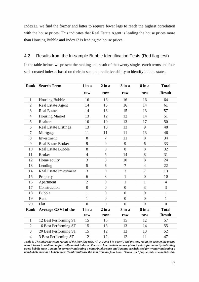
4.2 Results from the In-sample Bubble Identification Tests (Red flag test)

In the table below, we present the ranking and result of the twenty single search terms and four

self -created indexes based on their in-sample predictive ability to identify bubble states.

Rank Search Term 1 in a

row

2 in a

row

3 in a

row

8 in a

row

Total

Result

1 Housing Bubble 16 16 16 16 64

2 Real Estate Agent 14 15 16 14 61

3 Real Estate 14 13 15 13 57

4 Housing Market 13 12 12 14 51

5 Realtors 10 10 13 17 50

6 Real Estate Listings 13 13 13 9 48

7 Mortgage 11 11 11 13 46

8 Investment 8 7 11 8 34

9 Real Estate Broker 9 9 9 6 33

10 Real Estate Bubble 8 8 8 8 32

11 Broker 4 5 14 8 31

12 Home equity 3 3 10 8 24

13 Lending 5 6 7 4 22

14 Real Estate Investment 3 0 3 7 13

15 Property 6 3 1 0 10

16 Apartment 2 0 1 1 4

17 Construction 0 0 0 3 3

18 Bubble 1 0 0 0 1

19 Rent 1 0 0 0 1

20 Flat 0 0 0 0 0

Rank Average GSVI of the 1 in a

row

2 in a

row

3 in a

row

8 in a

row

Total

Result

1 12 Best Performing ST 15 15 15 12 57




Table 3: The table shows the results of the four flag tests, “1, 2, 3 and 8 in a row”, and the total result for each of the twenty

search terms in addition to four self-created indexes. The search terms/indexes are given 3 points for correctly indicating

a real bubble state, 1 point for correctly indicating a minor bubble state and 3 points are deducted for wrongly indicating a

non-bubble state as a bubble state. Total results are the sum from the four tests. “# in a row” flags a state as a bubble state

18

if GSVI for the specific search query is above a constant M times the GSVI level during the non-bubble period for #

consecutive quarters, where # = {𝟏, 𝟐, 𝟑 𝒂𝒏𝒅 𝟖}.

Table 3 shows the ranking and score from four different, in-sample prediction, tests based on

identifying the states that experienced a bubble for the twenty single search terms and the four

self-created indexes. To rank the different search terms and indexes we created a point system

where each query is given three points for correctly identifying a real bubble state, one point

for correctly identifying a minor bubble state and three points are deducted for erroneously

identifying a non-bubble state. The maximum number of points a search term may receive in

each of the four tests are; three points for each of the four bubble states, one point for each of

the six minor bubble states, equaling a maximum of eighteen points. We illustrate this through

an example, e.g. Housing Bubble has received sixteen points in all four tests for correctly

including all four real bubble states, four out of six minor bubble states and zero non-bubble

states.

From the results in Table 3, we see that GSVI for the two best performing search terms, namely

Housing Bubble and Real Estate Agent, outperforms the self-created indexes. We created four

different indexes consisting of the average GSVI for the twenty, twelve, six and three single

best-performing search terms to improve the robustness and the level of information captured.

Viewing the results, we see that this is not the case. From the full test results, we find that the

top two single search terms, in addition to getting the highest test score, are displaying more

robustness by performing rather well on a wide range of M values. Taking predictive ability,

robustness and simplicity into account, GSVI for single search terms seems most fitting as

housing bubble indicators. The search term Housing Bubble seems particularly suitable as a

bubble indicator as it performed best on all four tests. An advantage of using single queries,

such as Housing Bubble and Real Estate Agent over indexes, is that they can be combined and

hence increase the robustness and level of market information captured by the bubble indicator.

Also, GSVI for single search terms is easier to download and compute.

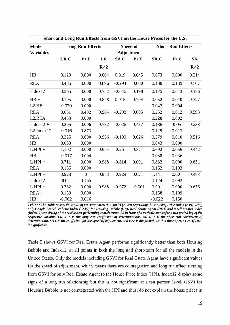
4.3 ECM Results for the United States

In the table below, we display the results from the regression of the house prices at level for

assessment of the long-run effects from Google searches and the result from the error correction

model to assess the short-run effects and the speed of adjustment from Google searches for the

whole of the United States.

19

Short and Long Run Effects from GSVI on the House Prices for the U.S.

Model

Variables

Long Run Effects Speed of

Adjustment

Short Run Effects

LR C P>Z LR

R^2

SA C P>Z SR C P>Z SR

R^2

HB 0.120 0.000 0.804 0.019 0.645 0.073 0.000 0.314

REA 0.486 0.000 0.896 -0.294 0.000 0.180 0.139 0.567

Index12 0.265 0.000 0.752 -0.046 0.198 0.175 0.013 0.176

HB +

L2.HB

0.195

-0.079

0.000

0.000

0.848 0.015 0.704 0.052

0.042

0.010

0.004

0.327

REA +

L2.REA

0.051

0.453

0.492

0.000

0.964 -0.298 0.005 0.252

0.228

0.012

0.002

0.593

Index12 +

L2.Index12

0.296

-0.016

0.006

0.873

0.782 -0.026 0.437 0.186

0.129

0.05

0.013

0.238

REA +

HB

0.325

0.053

0.000

0.000

0.956 -0.190 0.026 0.279

0.043

0.010

0.000

0.516

L.HPI +

HB

1.102

-0.017

0.000

0.004

0.974

-0.261

0.371

0.692

0.038

0.056

0.036

0.442

L.HPI +

REA

0.711

0.156

0.000

0.000

0.988

-0.814

0.001

0.832

0.162

0.000

0.103

0.651

L.HPI +

Index12

0.928

0.02

0

0.165

0.973

-0.929

0.021

1.441

0.124

0.001

0.092

0.483

L.HPI +

REA +

HB

0.732

0.153

-0.002

0.000

0.000

0.616

0.988

-0.972

0.001

0.991

0.158

-0.022

0.000

0.109

0.150

0.656

Table 5: The Table shows the result of an error correction model (ECM) regressing the Housing Price Index (HPI) using

only Google Search Volume Index (GSVI) for Housing Bubble (HB), Real Estate Agent (REA) and a self-created index

(index12) consisting of the twelve best-performing search terms. L2 in front of a variable stands for a two period lag of the

respective variable. LR R^2 is the long run coefficient of determinations, SR R^2 is the short-run coefficient of

determination, SA C is the coefficient for the speed of adjustment, and P>Z is the probability that the respective coefficient

is significant.

Table 5 shows GSVI for Real Estate Agent performs significantly better than both Housing

Bubble and Index12, at all points in both the long and short-term for all the models in the

United States. Only the models including GSVI for Real Estate Agent have significant values

for the speed of adjustment, which means there are cointegration and long run effect running

from GSVI for only Real Estate Agent to the House Price Index (HPI). Index12 display some

signs of a long run relationship but this is not significant at a ten percent level. GSVI for

Housing Bubble is not cointegrated with the HPI and thus, do not explain the house prices in

20

the long run. Housing Bubble is not an everyday term, and we expect search volume levels for

it to be relatively low except for in bubble phases as outlined by Aliber and Kindleberger

(2005). Therefore, we find it as no surprise that GSVI for Housing Bubble and the house prices

are not cointegrated. Index12 will have some of the same problems but to a lesser extent.

In the short run, both GSVI for Housing Bubble and Index12 display explanatory power on the

house prices. When including GSVI for both Housing Bubble and Real Estate Agent, we find

the results to be similar to those produced using only GSVI for Real Estate Agent. Substituting

Housing Bubble with a two period lag of Real Estate Agent yields improved results. This

indicates that inclusion of GSVI for Housing Bubble does not capture more of the market

information than Real Estate Agent do alone.

Real Estate Agent shows good predictive results, explaining the house prices in both the short

and long run. We also see that the speed of adjustment is relatively high for all models. When

only including GSVI for Real Estate Agent, without any lags, to explain the house prices, we

see the long run coefficient is 48.6%, and the long run coefficient of determinations (R^2) is

89.6%. The speed of adjustment is -29.4%, the short-run coefficient is 18%, and the short-run

coefficient of determinations is 56.7%. The r-squared values are high for both the short and

long run effects. The speed of adjustment is 29.4%, meaning that every period/quarter the error

correction term will move by 29.4% towards the long run equilibrium between GSVI for Real

Estate Agent and HPI. Taking into account that lags of the dependent variable is not included

shows the explanatory power of GSVI for Real Estate Agent on the HPI. When including a two

period lag of GSVI for Real Estate Agent, we see that the coefficient of determinations

increases to respectively 96.4% and 59.3%, while the speed of adjustment stays the same.

Substituting the two period lag of GSVI with a one period lag of the independent variable HPI

creates major changes. The coefficient of determinations increases to respectively 98.8% and

65.1%, and we see that the one period lag of HPI now stands for most of the explanation in

both the short and long run. Still, GSVI for Real Estate Agent is significant with a short run

coefficient of 15.6% and long run coefficient of 16.2%. We find the greatest change in the

speed of adjustment, which has increased to from -29.8% to -81.4%. These results show that

even simple linear models, including only GSVI and a one period, lagged variable of HPI can

explain the house prices.

21

4.4 ECM Results for all 50 States Using Only Google Searches

In the table below, we present the results from the regression of the house prices at level for

assessment of the long-run effects from GSVI for Real Estate Agent and the result from the

error correction model to assess the short-run effects, and the speed of adjustment from Google

searches for each the fifty states.

Linear Regression of HPI Using Only Google Searches. Long Run Effects

Model Variables L1.HPI P>Z GSVI P>Z L2.GSVI P>Z R^2

Average Results for the Real Bubble States

Only GSVI 0.734 0.000

0.709

GSVI + L2.GSVI 0.622 0.005 0.198 0.325 0.822

L1.HPI + GSVI 0.836 0.00 0.162 0.001 0.985

Average Results for the Minor Bubble States

Only GSVI 0.347 0.000

0.345

GSVI + L2.GSVI 0.54 0.089 -0.125 0.325 0.522

L1.HPI + GSVI 0.931 0.00 0.062 0.065 0.978

Average Results for the 30 states not defined

Only GSVI 0.278 0.029

0.496

GSVI + L2.GSVI 0.652 0.143 0.136 0.243 0.611

L1.HPI + GSVI 0.916 0.00 0.037 0.118 0.971

Average Results for the Non-Bubble States

Only GSVI 0.059 0.141

0.245

GSVI + L2.GSVI -0.002 0.346 0.071 0.298 0.241

L1.HPI + GSVI 0.967 0.00 0.003 0.384 0.932

Table 6: The Table shows the long run result of an error correction model (ECM) of the Housing Price Index (HPI) using

only Google Search Volume Index (GSVI) for Housing Bubble (HB) and Real Estate Agent (REA). L2 in front of a variable

stands for a two period lag of the respective variable. LR R^2 is the long run coefficient of determinations. LR MAE is the

Mean Absolute Error (MAE) between predicted value and real value of HPI at level.

ECM Using Only Google Searches to Explain the House Prices. Short Run Effects

Model Variables SA C P>Z L1

HPI

P>Z GSVI P>Z L2

GSVI

P>Z R^2

Average Results for the Real Bubble States

22

From Table 6 and Table 7, we see the model using only GSVI for Real Estate to regress the

house prices shows good in-sample predictive results. For the states experiencing a real bubble,

we see the average long run coefficient is 73.4% and significant, and the average long run

coefficient of determination is 70.9%. The average short-run coefficient is 17.6% and

significant at 10% confidence interval, and the average short-run coefficient of determination

is 36.3%. The speed of adjustment is -15.6%. Inspecting the full results more closely, we find

the in-sample prediction results to be significantly better for California and Florida than for

Nevada and Arizona (One can receive the results upon request). The short-run coefficient of

determination is respectively 57.3% and 50.8% for the former and respectively 15.2 and 21.9%

for the latter.

Including a two period lag of GSVI for Real Estate Agent increases the long run coefficient of

determination to 82.2%, while decreasing the short run coefficient of determination and speed

of adjustment to respectively 34.3% and -10.1%. Substituting the two-period lag with a one

Only GSVI -0.16 0.003 0.176 0.094

0.36

GSVI + L2.GSVI -0.10 0.065 0.201 0.106 0.17 0.158 0.34

L1.HPI + GSVI -0.58 0.009 1.074 0.000 0.12 0.050 0.71

Average Result for the Minor Bubble States

Only GSVI -0.08 0.068 0.003 0.515

0.17

GSVI + L2.GSVI -0.07 0.185 0.062 0.402 0.03 0.344 0.17

L1.HPI + GSVI -0.69 0.047 1.126 0.004 0.02 0.382 0.53

Average Results for the 30 states not defined

Only GSVI -0.09 0.123 0.045 0.319

0.18

GSVI + L2.GSVI -0.09 0.135 0.043 0.356 0.04 0.268 0.19

L1.HPI + GSVI -0.84 0.088 1.127 0.018 0.05 0.335 0.38

Average Results for the Non-Bubble States

Only GSVI -0.04 0.334 0.015 0.472

0.08

GSVI + L2.GSVI -0.04 0.352 0.013 0.46 0.02 0.495 0.11

L1.HPI + GSVI -0.96 0.159 0.928 0.055 0.01 0.538 0.22

Table 7: The Table shows the short run result of an error correction model (ECM) of the Housing Price Index (HPI) using

only Google Search Volume Index (GSVI) for Real Estate Agent (REA). L2 in front of a variable stands for a two period lag

of the respective variable. SR R^2 is the short-run coefficient of determination. SR MAE is the Mean Absolute Error between

predicted change in HPI and real value. SA C is the coefficient for speed of adjustment and P>Z is the probability that the

respective coefficient is significant.

23

period lag of the dependent variable HPI creates more major changes. Both the long and short

run coefficient of determinations increases to respectively 98.5% and 71.4%, while the speed

of adjustment increases to -58.1%. We find the same throughout the groups of real, minor, and

non-bubble states.

Evaluating the other state groups in Table 6 and Table 7, we find the coefficient of determinants

for both the long and short run to be largest for the real bubble states and least for the non-

bubble states. For the minor bubble states and the thirty states not defined as either bubble nor

non-bubble states, we find the opposite result. This might be explained by two factors; first is

the general bubble that existed globally in the U.S. housing market. Secondly, we suspect the

size of the population in each state to affects the quality of the respective Google Trend data in

the state.

In our work with this paper, we also constructed a Vector error correction model (VECM) to

investigate the relationship between Google search and the house prices at state level. Due to

the rigidity of the model and problems interpreting the results from the baseline models, which

had several long run relationships, we decided to use other models. Never the less, the result

from the VECM was coinciding with those presented above.

4.5 ECM Results for all 50 States Using the Baseline Variables

In this section, we will go through and compare the results from the baseline model with and

without the inclusion of Google searches. To say something about how valuable it is to include

Google search volume in a model for estimating the house prices, we compare the baseline

model not only to a model including Google search volume, but also with a model including

the Consumer Confidence Index (CCI). The Consumer Confidence Index is a well-known and

widely used leading indicator and should be a good benchmark.

Model

Description

LR

R^2

LR

MAE

SR

R^2

SR

MAE

SA C P>Z

Average results for the Real Bubble States

Baseline Model 0.992 1.494% 0.816 1.153% -0.616 0.006

Baseline GSVI Model 0.993 1.440% 0.834 1.146% -0.664 0.002

Baseline CCI Model 0.992 1.492% 0.824 1.182% -0.594 0.008

Average results for the Minor Bubble States

24

Baseline Model 0.987 1.017% 0.739 0.847% -0.695 0.004



Average results of the Thirty States not Defines as either Bubble nor non-bubble

Baseline Model 0.979 0.879% 0.634 0.772% -0.782 0.003



Average results for the Non-Bubble States

Baseline Model 0.944 0.715% 0.488 0.661% -0.858 0.009



Table 8: The table summarises three different versions of a baseline housing price model with Disposable Personal Income,

Housing Permits Authorised, Unemployment Rate, Interest Rate and Population as explanatory variables. Also, a one

period lag of the dependent variable is included. The “Baseline Model” includes the former variables, “Baseline Model

Including GSVI” includes Google Search Volume Index (GSVI) for Real Estate Agent in addition to the other variables

and “Baseline Model Including CCI” includes Consumer Confidence Index (CCI) instead of Google searches. In addition

to this these three Baseline Models, we have “Model Only Using GSVI and L1.HPI” which is the best performing model

using only GSVI for Real Estate and a one period lag of the dependent variable the Housing Price Index (HPI). The four

models are assessed after the following criteria’s; LR R^2 is the adjusted long run coefficient of determinations, LR MAE

is the Mean Absolute Error (MAE) between predicted value and real value for HPI at level, SR R^2 is the adjusted short-

run coefficient of determination, SR MAE is the MAE between predicted change in HPI and real value, SA C is the

coefficient for speed of adjustment and P>Z is the probability that the coefficient is significant.

Viewing the result in Table 8, we see that all points of criteria are improved when including

GSVI for Real Estate Agent in the baseline model. The adjusted coefficient of determination

is increased for both the long and short run, and the speed of adjustment is both higher and

more significant. These results apply for the real, minor and non-bubble states. In addition to

the thirty states not defined as either bubble nor non-bubble states.

For the real bubble states, including GSVI for Real Estate Agent reduced the mean absolute

error (MAE) on average with respectively 0.61% for the long run in-sample prediction and

3.78% for the short run in-sample prediction. For the minor bubble states, the MAE was

reduced with respectively 4.42% for the long run in-sample prediction and 3.78% for the short

run in-sample prediction. In the thirty states not defined as either bubble nor non-bubble states,

there was the following improvement for the long and short run in-sample prediction MAE

with respectively 3.1% and 2.97%. Last, for the non-bubble states, the average improvement

in reduced MAE was respectively 1.11% and 1.21%.

Substituting Google searches with the Consumer Confidence Index (CCI) yields significantly

worse results on all points of criteria except one, the short run MAE for the non-bubble states

are on average reduced by 0.15%. Including CCI in the Baseline Model improves the MAE in

25

both the long and short run but display a decreased coefficient of determination and lower

speed of adjustment. Based on the results above, we conclude that GSVI for Real Estate Agent

improves both the fitness of the Baseline Model and reduces the MAE of the in-sample

prediction in both the long and short run. Also, the inclusion of GSVI for Real Estate Agent

yields significantly better results than the inclusion of CCI.

As described in the previously section, we also constructed a vector error correction model

(VECM) using all the baseline variables. We included GSVI for Real Estate Agent and

Index12, separately, for all the 50 states. Our findings was coinciding with those above.

Comparing the result from the model using only GSVI for Real Estate Agent and a one period

lag of the dependent variable with the Baseline Model, we find the latter to perform better. The

former model shows higher speed of adjustment for the thirty states not defined as either bubble

nor non-bubble states and the non-bubble states. Assessing the long run coefficient of

determination results, we find them to be coinciding with slightly better results for the Baseline

Model. The major difference in performance is in the short run, where the Baseline Model

display better fit. Still, we find the in-sample prediction results for such a simple model to be

rather good.

5 Conclusion

The aim of this paper is to test whether Google search volume indices can be used to predict

house prices and to identify bubbles in the housing market. We use Google Trends data, and

tested several Google Search Volume Indexes (GSVI) and find good in-sample predictive

abilities. Taking predictive abilities, simplicity and robustness into consideration, we conclude

that the best candidate as a housing bubble indicator is GSVI for Housing Bubble. When

optimising to detect all the states experiencing a bubble, GSVI for Housing Bubble erroneously

included only one non-bubble state and when optimising on not wrongly including any non-

bubble states, it detected all four real bubble states and four out of six minor bubble states. It

repeatedly produced the same results for a wide variety of tests. For the states experiencing a

housing bubble, GSVI for Housing Bubble displays relative low search volume levels, without

any trends both before and after the bubble, but during the actual bubble period the search

volume levels “explodes”, increasing several 100%. Search volume levels for Housing Bubble

26

globally in the U.S. displayed the same characteristics, leading the house prices and strongly

indicating a real estate bubble. The extreme characteristics of GSVI for Housing Bubble during

a bubble period, means there is no need to adjust the data for neither seasonally affects nor

trends. Thus, simplifying the surveillance of the indicator.

GSVI for Real Estate Agent displays the highest correlation with the Housing Price Index (HPI)

and yield the best in-sample predictive results of the house prices in both the short and long

run. Also, GSVI for Real Estate Agent and the HPI are cointegrated in 45 out of 50 states, and

the former is leading the house prices in both the bubble and the non-bubble period. When

testing the relationship between GSVI for Real Estate Agent and the HPI, we found both short

and long-term effects running from the former to the latter. These effects were significant in

states experiencing a real, minor and no bubble. Constructing a simple linear model using only

GSVI for Real Estate Agent and a one period lag of the dependent variable, HPI, produced

good in-sample prediction results. The fit of the model and the mean absolute error results was

best for the states experiencing a real bubble, followed by the states experiencing a minor

bubble and least for the states experiencing no bubble. Predicting the house prices, using the

same model, globally in the U.S. gave even better results than for the states experiencing a real

housing bubble.

Including GSVI for Real Estate Agent in our Baseline error correction model for the house

prices, improved all points of criteria. The adjusted coefficient of determination increases for

both the short and long run and the speed of adjustment is higher and more significant.

Substituting Google searches with the well-established Consumer Confidence Index yielded

worse result for all assessments. The results are valid for the real, minor and non-bubble states.

In addition to the thirty states not defined as either bubble nor non-bubble states.

Based on the results found in this paper, we conclude that GSVI for Housing Bubble can be a

strong housing bubble indicator while GSVI for Real Estate Agent can predict the housing

trend and be included in price models to improve their predictive abilities at state levels.

27

Reference List

Benjamin, J., Chinloy, P. and Jud, D. (2004), ”Real estate versus financial wealth in

consumption”. In: Journal of Real Estate Finance and Economics 29, pp. 341-354.

Bracke, P. (2013), ”How long do housing cycles last? A duration analysis for 19 OECD

countries”. In: Journal of Housing Economics Vol. 22 No. 3, pp. 213–230.

Brunnermeier, M.K. and Oehmke, M. (2012), “Bubbles, Financial Crises, and Systemic

Risk”, National Bureau of Economic Research, Working Paper No. 18398.

Campbell, J. and J. Cocco (2004), “How Do Housing Price Affect Consumption? Evidence

from Micro Data”, Harvard Institute of Economic Research, Discussion Paper No. 2045.

Case, K.E., Quigley, J. and Shiller R. (2001), “Comparing wealth effects: the stock market

versus the housing market”, National Bureau of Economic Research, Working Paper No.

8606.

Case, K.E. and Shiller, R.J. (2004), “Is there a Bubble in the Housing Market?”, Cowless

foundation paper no. 10 89.

Chen, B., Schoeni, R. and Stafford, F. (2012), “Mortgage Distress and Financial Liquidity:

How U.S. Families are Handling Savings, Mortgages and Other Debts”, Technical Series

Paper 12-02, Survey Research Center, Institute for Social Research, University of

Michigan.

Choi, H., and H. R. Varian. 2012, “Predicting the Present with Google Trends”,

Economic Record, 88:1 pp 2-9.

Damien, C. and Ahmed, B. H. A. 2013, “Ahmed, Predicting Financial Markets with Google

Trends and Not so Random Keywords” (August 14, 2013). Available at

SSRN: https://ssrn.com/abstract=2310621 or http://dx.doi.org/10.2139/ssrn.2310621.

Ettredge, M., Gerdes, J. and G. Karuga (2005), “Using web-based search data to predict

macroeconomic statistics”, Communications of the ACM, 48(11):87–92.

Goel, S., Hofman, J.M., Lahaie, S., Pennock, D.M., and Watts D.J. (2010), “Predicting

consumer behavior with web search”, Proceedings of the National Academy of Sciences,

7(41):17486–17490, Sep 27 2010.

Harding, D. and Pagan, A. (2002), ”Dissecting the cycle: a methodological investigation”,

Journal of Monetary Economics Volume 49, Issue 2, pp. 365–381

Horrigan, J. B. (2008),“The Internet and Consumer Choice: Online Americans Use Different

Search and Purchase Strategies for Different Goods”, Technical Report, Pew Internet and

American Life Project.

28

Kindleberger, C. and R. Aliber, R. (2005), "Manias, Panics and Crashes –A History of

Financial Crises", John Wiley and Sons, Hoboken, NJ.

Kuruzovich, J., S. Viswanathan, R. Agarwal, S. Gosain, and S. Weitzman. (2008)

“Marketspace or Marketplace? Online Information Search and Channel Outcomes in Auto

Retailing”, Information Systems Research 19 (2): 182–201.

Lind, H. (2009). “Price bubbles in housing markets: concept, theory and indicators”. In:

International Journal of Housing Markets and Analysis Vol. 2 No. 1, pp. 78-90.

Oust, A. and Hrafnkelsson, K. (2017) ''What is a housing bubble?'', Economics Bulletin,

Volume 37, Issue 2, pages 806-836

Pentland, A. S. (2010), Honest Signals. Cambridge, MA: MIT Press.

Preis, T., Moat, H. S. and Stanley, H. E. (2013), “Quantifying Trading Behavior in Financial

Markets Using Google Trends”. Scientific Reports, 3, Article number 1684.

Preis, T., Reith, D. and Stanley, H. E. (2010) “Complex dynamics of our economic life on

different scales: insights from search engine query data”, Philosophical Transactions of the

Royal Society of London, 5707–19.

Wu, L. and Brynjolfsson, E. (2015) The Future of Prediction How Google Searches

Foreshadow Housing Prices and Sales, Chapter in NBER book Economic Analysis of the

Digital Economy, editors Avi Goldfarb, Shane M. Greenstein, and Catherine E. Tucker,

editors (p. 89 - 118).

29

Appendix A

The 50 United States Sorted After their Total Price Fall from Top to Bottom

Rank State 3 years 5 years Top HPI Peak Bottom Trough Price Fall

1 Nevada 65.1% 79.5% 491.2 Q1 2006 191.4 Q2 2012 -61.0%

2 Arizona 55.2% 68.8% 506.2 Q4 2006 247.4 Q3 2011 -51.1%

3 Florida 50.2% 78.4% 570.9 Q4 2006 280.4 Q2 2012 -50.9%

4 California 56.2% 84.9% 770.1 Q2 2006 402.7 Q1 2012 -47.7%

5 Michigan 3.0% 9.3% 394.5 Q2 2005 240.1 Q2 2012 -39.1%

6 Rhode Island 36.5% 72.5% 726.0 Q1 2006 448.2 Q4 2013 -38.3%

7 Maryland 42.5% 72.1% 630.2 Q4 2006 420.4 Q1 2013 -33.3%

8 Idaho 35.3% 40.0% 398.5 Q1 2007 266.7 Q2 2011 -33.1%

9 Oregon 34.2% 45.1% 533.6 Q2 2007 357.7 Q2 2012 -33.0%

10 Washington 36.1% 43.7% 580.0 Q1 2007 396.1 Q2 2012 -31.7%

11 Georgia 6.1% 9.8% 382.7 Q4 2006 262.0 Q2 2012 -31.5%

12 New Jersey 26.3% 53.2% 682.8 Q4 2006 469.2 Q4 2013 -31.3%

13 New Hampshire 21.0% 44.0% 561.8 Q1 2006 388.8 Q1 2013 -30.8%

14 Minnesota 14.8% 30.2% 442.7 Q1 2006 306.4 Q2 2012 -30.8%

15 Connecticut 25.6% 43.1% 560.8 Q1 2006 389.8 Q1 2014 -30.5%

16 Illinois 11.9% 21.5% 440.0 Q4 2006 306.1 Q1 2013 -30.4%

17 Delaware 28.7% 47.6% 591.9 Q4 2006 420.2 Q1 2014 -29.0%

18 Massachusetts 24.4% 50.2% 880.5 Q2 2005 628.6 Q4 2012 -28.6%

19 Ohio 2.8% 7.1% 328.2 Q2 2005 241.4 Q1 2014 -26.4%

20 Hawaii 46.5% 78.9% 631.3 Q1 2007 466.4 Q2 2012 -26.1%

21 Virginia 34.9% 54.9% 552.1 Q4 2006 408.0 Q2 2012 -26.1%

22 New Mexico 26.6% 34.1% 382.6 Q1 2007 288.6 Q1 2014 -24.6%

23 Utah 30.4% 30.2% 439.9 Q3 2007 333.4 Q4 2003 -24.2%

24 New York 19.8% 42.0% 760.4 Q4 2006 577.9 Q1 2014 -24.0%

25 Maine 15.6% 34.9% 600.6 Q4 2006 458.3 Q1 2014 -23.7%

26 Wisconsin 12.7% 18.6% 387.0 Q1 2006 297.3 Q1 2014 -23.2%

27 Missouri 6.7% 13.5% 351.3 Q4 2006 275.8 Q1 2014 -21.5%

28 South Carolina 12.7% 15.4% 395.0 Q4 2006 310.5 Q1 2014 -21.4%

29 North Carolina 10.2% 12.7% 387.6 Q2 2007 310.0 Q4 2013 -20.0%

30 Alabama 11.5% 14.5% 349.1 Q2 2007 280.7 Q4 2013 -19.6%

31 Mississippi 11.9% 13.4% 301.6 Q1 2007 243.7 Q4 2013 -19.2%

32 Pennsylvania 19.3% 32.0% 463.4 Q4 2006 375.7 Q1 2014 -18.9%

33 Indiana 1.5% 4.8% 306.5 Q2 2005 249.8 Q1 2014 -18.5%

30

34 Colorado 14.2% 21.7% 427.9 Q4 2006 349.5 Q1 2012 -18.3%

35 Vermont 23.5% 40.5% 533.9 Q4 2006 440.3 Q1 2014 -17.5%

36 Tennessee 9.7% 12.8% 350.6 Q2 2007 292.1 Q1 2013 -16.7%

37 Montana 20.8% 35.8% 431.5 Q3 2007 363.1 Q2 2012 -15.9%

38 Arkansas 9.3% 13.6% 299.2 Q1 2007 252.1 Q2 2012 -15.7%

39 West Virginia 13.0% 16.8% 259.5 Q4 2006 219.0 Q1 2013 -15.6%

40 Kentucky 3.3% 6.6% 340.4 Q4 2006 292.2 Q1 2014 -14.1%

41 Kansas 2.6% 6.3% 280.6 Q4 2006 241.9 Q1 2014 -13.8%

42 Nebraska 4.7% 7.4% 302.5 Q2 2005 262.2 Q4 2012 -13.3%

43 Wyoming 24.2% 38.6% 323.8 Q3 2007 281.9 Q1 2012 -13.0%

44 Louisiana 15.2% 21.1% 284.2 Q1 2007 251.4 Q1 2013 -11.5%

45 Alaska 22.1% 31.5% 332.6 Q1 2007 294.7 Q2 2012 -11.4%

46 Texas 6.0% 10.0% 257.5 Q2 2007 232.7 Q1 2012 -9.6%

47 Iowa 5.4% 9.6% 289.8 Q2 2005 270.0 Q3 2008 -6.8%

48 South Dakota 3.9% 6.8% 331.1 Q1 2007 309.1 Q3 2012 -6.6%

49 Oklahoma 2.5% 5.2% 231.8 Q1 2007 222.6 Q3 2008 -4.0%

50 North Dakota 12.4% 19.4% 280.0 Q1 2007 271.6 Q3 2008 -3.0%

Table appendix A: The table display the fifty states sorted according to their price fall from the peak to the trough.”3 years”

and “5 years” is the percentage price increase the last three and five years before the price top in each respective state.

“Top HPI” and “Bottom” is the highest and lowest value for the Housing Price index (HPI) in each respective state. “Peak”

and “Trough” is the quarter and year for the highest and lowest value of HPI. “Price Fall” is the percentage price fall

from peak to trough in each respective state.

Appendix B

Search Terms

List of Alphabetically Sorted Search Terms

A Acres, Acres of Land, Affordable Housing, Analyst

B Backyard, Beach Front, Broker, Bubble, Building a House, Building Cost, Buying Out

C CBS Constructed Homes, Consumer Loans, Consumer Credit, Consumer Lending, Condos,

Credit

D Debt, Disposable Income, Down Payment, Duplex Home, Dwelling, Dwellings

E Equity, Equity Requirement

F Financial, Financial Analysis, First Time Homebuyer, Future Interest

G Gated Communities, GDP

H Home Equity, Home Equity Loan, Homes in up and Coming Communities, House Analysis,

I Income, Income Change, Income Increase, Income Raise, Increasing Property Prices

Increasing Real Estate Prices, Inflation, Installments, Interest Forecast, Interest,

31

Interest Rate

L Land Price, Land Prices, Leasing, Lending, Lending Standard, Low Down Payment, Low

M Middle Class Homes, Mortgage, Mortgage Payment, Mortgage Requirements

N Net Immigration, New Buildings, Newly Renovated, Number of Completed Homes

O One Story Home, Overpriced, Overvaluation

P Part Payment, Patio, Peak, Pet Approval, Pool, Pricing, Property Bubble, Property, Property

Investment, Property Tax, Property Under Construction, Population

R Raising Property, Real Estate, Real Estate Advisor, Real Estate Agent, Real Estate Bubble,

Real Estate Broker, Realtor, Real Estate Listings

S Salary Increase, Salary Change, Salary Raise, School District, Second Mortgage

T Turmoil, Two Storey Home, Two Storey House

U Unemployment, Unemployment Rate

V Vacation House, Valuation

W Wage, Wages, Wage Increase, Wage raise, Waterfront Property

Z Zero Interest Rate

Table appendix B: The table presents the 204 search term, originally tested, sorted alphabetically.

Appendix C

Correlation Housing Bubble - HPI Real Estate Agent - HPI Index12 - HPI

State Name WP BP NP WP BP NP WP BP NP

Nevada 0.486 0.301 -0.11 0.874 0.794 0.326 0.78 0.923 -0.695

Arizona 0.855 0.701 0.397 0.846 0.902 -0.048 0.73 0.886 -0.718

Florida 0.887 0.776 0.478 0.957 0.955 0.955 0.84 0.922 -0.489

California 0.925 0.938 0.793 0.963 0.968 0.898 0.78 0.920 -0.465

Ave RBS 0.788 0.679 0.390 0.910 0.905 0.533 0.78 0.913 -0.592

Maryland 0.919 0.638 0.633 0.940 0.820 0.736 0.88 0.787 0.182

Oregon 0.697 0.308 -0.22 0.620 0.118 -0.624 0.67 0.750 -0.540

Washington 0.766 0.385 0.617 0.817 0.573 0.433 0.64 0.497 -0.416

New Jersey 0.939 0.686 0.407 0.884 0.746 0.576 0.89 0.797 0.478

Virginia 0.854 0.479 -0.41 0.860 0.921 0.721 0.81 0.834 -0.585

Connecticut 0.723 0.577 0.366 0.880 0.873 -0.285 0.91 0.815 0.722

Ave MBS 0.816 0.512 0.231 0.833 0.675 0.260 0.80 0.747 -0.027

Kansas N/A N/A N/A 0.752 0.729 -0.012 0.66 0.436 -0.296

Nebraska N/A N/A N/A 0.705 0.658 0.444 0.44 0.232 -0.507

32

Wyoming N/A N/A N/A 0.544 0.647 0.493 0.19 0.231 -0.505

Louisiana N/A N/A N/A 0.675 0.532 -0.140 0.54 0.321 -0.263

Alaska N/A N/A N/A 0.628 0.332 0.141 0.34 0.152 -0.409

Texas 0.045 0.114 0.464 0.271 0.060 0.848 0.25 0.073 -0.576

Iowa N/A N/A N/A 0.753 0.591 0.178 0.62 0.175 -0.212

South Dakota N/A N/A N/A 0.360 0.198 0.350 -0.37 0.123 -0.695

Oklahoma N/A N/A N/A 0.563 0.468 -0.488 0.36 -0.14 -0.402

North Dakota N/A N/A N/A 0.307 -0.09 0.616 -0.23 0.338 -0.726

Average NBS N/A N/A N/A 0.556 0.412 0.243 0.28 0.202 -0.459

Table appendix C: The table shows the correlation between: Google Search Volume Index (GSVI) for Housing Bubble and

the Housing Price Index (HPI), GSVI for Real Estate Agent and HPI, GSVI for Index12 and HPI. The correlation is

displayed for the whole period (WP), Q1 2004 – Q3 2016, the bubble period (BP), Q1 2004 – Q2 2010, and the normal

period (NP), Q3 2010 – Q3 2016. The correlation is calculated for the states defined as real bubble states (RBS), minor

bubble states (MBS) and non-bubble states (NBS). Also, the average for each of the three groups is calculated.. N/A means

there are missing GSVI data for the respective state.

Appendix D

D.1 Stationarity Test of the Variables at Level for all 50 States

Country General Variables ln CCI ln IR ln DPI

t-statistics -1.493 -0.843 -1.234

Table appendix D 1.1: The table shows the results from the Dickey-Fuller Generalized Least Square unit root test of the

following time series at Level. The natural logarithm to Consumer Confidence Index (CCI), 1 + Interest Rate in percentage

(IR) and Disposable Personal Income (DPI). The three time-series are all general for the United States.

State Specific Variables ln HPI ln UR ln DPO ln HPA ln GSVI

State Name t-statistics t-statistics t-statistics t-statistics t-statistics

Nevada -1.4 -3.1 * -2.3 -1.4 -1.2

Arizona -1.5 -3.9 *** -2.8 -1.1 -0.9

Florida -1.3 -2.9 -2 -1 -0.9

California -1.7 -3.2 ** -2.2 -0.9 -1.4

Maryland -1.3 -2.3 -2.1 -1.7 -1.4

Idaho -1.4 -1.3 -1.7 -1.9 -1.7

Oregon -1.4 -1.3 -1.7 -1.9 -1.4

Washington -1.4 -3.3 ** -2.1 -1.8 -1.0

Hawaii -1.3 -2.7 -2.2 -1.5 -5.2 ***

Virginia -1.3 -2.1 -2.2 -1.2 -1.6

Rhode Island -0.9 -2.6 -2.5 -1.5 -1.9

33

Michigan -0.8 -2.2 -1.6 -1.7 -2.4 **

Georgia -1.0 -1.8 -1.2 -1.0 -0.6

New Jersey -1.1 -2.6 -2.1 -1.5 -1.0

New Hampshire -0.8 -2.5 -2.1 -2.2 * -4.5 ***

Minnesota -0.9 -2.2 -3.7 ** -2.4 ** -1.3

Connecticut -0.5 -2.1 -2.7 -1.8 -1.5

Illinois -0.7 -1.9 -3.3 ** -1.2 -1.5

Delaware -1.0 -2.7 -2.7 -1.6 -0.5

Massachusetts -1.0 -2.8 -2.2 -1.6 -1.6

Ohio -0.6 -2.1 -2.5 -1.8 -1.1

New Mexico -1.1 -2.8 -2.5 -1.0 -1.0

Utah -1.5 -2.1 -3.8 *** -1.9 -1.9

New York -1.1 -2.6 -2.8 -2.3 ** -1.6

Maine -1.0 -2.3 -2.8 -2.5 ** -2.1 *

Wisconsin -0.8 -2.5 -2.4 -2.3 ** -0.8

Missouri -0.9 -2.8 -1.8 -1.4 -0.9

South Carolina -1.3 -2.1 -3.2 ** -1.4 -1.2

Alabama -1.0 -2.5 -3.2 ** -0.9 -1.0

Mississippi -0.9 -1.6 -3.4 ** -1.3 -2.5 **

Pennsylvania -1.2 -2.1 -2.4 -1.7 -2.2 *

Indiana -0.7 -1.9 -3.0 * -1.9 -2.0 *

Colorado -0.6 -2.5 -3.6 ** -1.4 -1.7

Vermont -1.0 -1.9 -4.2 *** -3.2 *** -2.3 **

Tennessee -1.2 -2.1 -1.7 -1.1 -1.1

Montana -0.8 -2.1 -3.0 * -2.9 *** -4.4 ***

Arkansas -1.1 -2.2 -3.1 * -1.9 -1.6

West Virginia -1.1 -2.3 -3.0 * -1.8 -3.4 ***

Kentucky -1.0 -2.1 -3.4 ** -1.6 -2.4 **

Kansas -1.0 -2.5 -2.8 -1.8 -1.6

Nebraska -1.1 -2.4 -2.2 -3.1 *** -2.0 *

Wyoming -0.8 -2.7 -2.6 -3.8 *** -1.8

Louisiana -1.2 -2.7 -2.4 -1.8 -1.3

Alaska -0.9 -2.5 -2.7 -3.9 *** -2.5 **

Texas 0.0 -2.6 -2.2 -1.6 -1.0

Iowa -1.2 -2.8 -2.2 -3.4 *** -3.2 ***

South Dakota -0.3 -2.5 -2.0 -4.9 *** -2.1 *

Oklahoma -1.3 -3.5 *** -2.6 -1.7 -0.7

North Dakota -1.4 -2.6 -2.6 -3.0 *** -5.1 ***

Table appendix D1.2: The table show the result from the Dickey-Fuller Generalized Least Square (DF-GLS) unit root test

of the following time series in Level. The natural logarithm to Housing Price Index (HPI), 1+Unemployment Rate in

percentage (UR), Housing Permits Authorized (HPA), Population (PO) and Google Search Volume Index (GSVI). The five

time-series are state specific for each of the 50 states. The DF-GLS tests are performed with the No Trend option for all

variables except Unemployment Rate.

34

D.2 Stationarity Test of the First Differenced Variables for all 50 States

Country General Variables ∆ ln CCI ∆ ln IR ∆ ln DPI

t-statistics -5.333 *** -3.557 *** -4.968 ***

Table appendix D2.1: The table shows the results from the Dickey-Fuller Generalized Least Square unit root test of the

following first differenced time series. The natural logarithm to Consumer Confidence Index (CCI), 1 + Interest Rate in

percentage (IR) and Disposable Personal Income (DPI). The three time-series are general for the United States. The tests

are performed with the no trend option for all variables.

State Specific Variables ∆ ln HPI ∆ ln UR ∆ ln DPO ∆ ln HPA ∆ ln GSVI

States t-statistics t-statistics t-statistics t-statistics t-statistics

Nevada -1.8 -1.6 -5.1 *** -6.5 *** -8.4 ***

Arizona -2 * -2 * -5.6 *** -4.2 *** -5.5 ***

Florida -2.1 * -1.9 * -5.0 *** -3.2 *** -5.1 ***

California -1.9 * -1.6 -2.6 *** -3.4 *** -4.9 ***

Maryland -2.1 * -2.7 *** -2.4 *** -5.8 *** -3.8 ***

Idaho -2.9 *** -2.4 ** -5.0 *** -5.1 *** -3.9 ***

Oregon -2.9 *** -2.4 ** -5.0 *** -5.1 *** -8.0 ***

Washington -2.3 ** -2.8 *** -2.5 *** -5.0 *** -4.9 ***

Hawaii -1.9 * -2.6 *** -2.4 *** -6.6 *** -9.3 ***

Virginia -2.6 *** -2.7 *** -2.4 *** -5.5 *** -4.6 ***

Rhode Island -2.5 ** -2.7 *** -2.72 -5.0 *** -6.0 ***

Michigan -4.4 *** -3.6 *** -5.0 *** -5.9 *** -1.2

Georgia -4.0 *** -2.1 * -5.2 *** -6.7 *** -3.5 ***

New Jersey -2.6 *** -2.8 *** -3.1 *** -4.6 *** -1.6

New Hampshire -3.1 *** -3.6 *** -4.6 *** -5.5 *** -2.8 ***

Minnesota -4.6 *** -2.9 *** -3.5 *** -3.9 *** -6.6 ***

Connecticut -2.9 *** -2.5 *** -3.5 *** -4.7 *** -4.1 ***

Illinois -3.2 *** -3.1 *** -4.9 *** -4.4 *** -3.7 ***

Delaware -2.7 *** -3.0 * -4.9 *** -8.3 *** -0.8

Massachusetts -3.1 *** -2.2 * -2.9 * -3.0 *** -3.4 ***

Ohio -5.4 *** -3.0 *** -2.9 * -4.7 *** -5.9 ***

New Mexico -2.9 *** -3.9 *** -4.7 *** -6.4 *** -7.9 ***

Utah -3.1 *** -2.9 *** -6.6 *** -5.1 *** -4.5 ***

New York -3.1 *** -2.6 ** -3.2 ** -3.9 *** -1.4

Maine -3.0 *** -3.6 *** -5.0 *** -3.8 *** -2 *

Wisconsin -3.7 *** -3.6 *** -4.7 *** -5.1 *** -2.3 **

Missouri -4.3 *** -2.4 ** -5.0 *** -5.6 *** -4.5 ***

South Carolina -4.1 *** -3.2 *** -2.9 * -5.2 *** -2.5 **

Alabama -4.1 *** -3.3 *** -2.9 * -8.0 *** -4.0 ***

Mississippi -4.1 *** -3.3 *** -4.9 *** -9.1 *** -7.3 ***

Pennsylvania -3.2 *** -3.0 *** -3.0 * -5.2 *** -4.5 ***

35

Indiana -5.9 *** -3.3 *** -2.9 *** -4.9 *** -2.2 ***

Colorado -3.6 *** -1.8 -3.0 * -4.8 *** -7.5 ***

Vermont -2.9 *** -4.0 *** -6.5 *** -4.4 *** -7.3 ***

Tennessee -4.0 *** -3.8 *** -5.0 *** -5.7 *** -6.1 ***

Montana -3.0 *** -2.9 *** -3.5 *** -4.6 *** -5.9 ***

Arkansas -3.6 *** -3.8 *** -7.2 *** -4.5 *** -4.6 ***

West Virginia -4.4 *** -4.5 *** -3.3 ** -6.2 *** -1.9

Kentucky -5.1 *** -3.3 *** -4.9 *** -7.3 *** -6.6 ***

Kansas -4.9 *** -2.6 *** -3.5 ** -5.6 *** -9.7 ***

Nebraska -4.6 *** -3.0 *** -2.4 -3.9 *** -8.4 ***

Wyoming -2.6 *** -3.6 *** -2.9 * -5.9 *** -8.2 ***

Louisiana -4.0 *** -5.7 *** -3.5 *** -4.1 *** -4.6 ***

Alaska -3.4 *** -3.2 *** -3.7 *** -4.2 *** -3.9 ***

Texas -3.5 *** -2.6 *** -2.6 -4.8 *** -4.8 ***

Iowa -5.0 *** -3.2 *** -2.4 -4.4 *** -10.8 ***

South Dakota -4.2 *** -3.6 *** -2.4 -9.3 *** -4.3 ***

Oklahoma -5.0 *** -3.5 *** -3.2 ** -7.5 *** -2.0 *

North Dakota -4.3 *** -4.9 *** -2.7 -3.7 *** -10.0 ***

Table appendix D2.1: The table shows the results from the Dickey-Fuller Generalized Least Square (DF-GLS) unit root

test of the first difference of the following time series. The tests are performed with the No Trend option for all variables.

The natural logarithm to Housing Price Index (HPI), 1+Unemployment Rate in percentage (UR). Housing Permits

Authorized (HPA), Population (PO) and Google Search Volume Index (GSVI). The five time-series are state specific for

each of the fifty states. The DF-GLS tests are performed with the No Trend option for all variables except Unemployment

Rate.

Appendix E

E.1 Test of Cointegration among all Variables for all 50 States

Johansen Cointegration Test

Maximum

Rank

Standard Model CCI Model GSVI Model

5% Critical Value 5% Critical Value 5% Critical Value

0 94.15 124.24 124.24

1 68.52 94.15 94.15

2 47.21 68.52 68.52

3 29.68 47.21 47.21

4 15.41 29.68 29.68

5 3.76 15.41 15.41

6 3.76 3.76

State Name No of

CR

Trace

Statistics

No of

CR

Trace

Statistics

No of

CR

Trace

Statistics

Nevada 2 40.3627 3 43.7198 3 41.3831

Arizona 3 23.9541 3 45.1838 4 23.6582

Florida 3 28.8519 3 44.5998 4 28.8787

36

California 3 25.6202 5 10.3180 5 10.3595

Maryland 2 45.2226 4 24.8237 3 43.2934

Idaho 3 16.3943 3 41.7381 4 16.1368

Oregon 3 16.3943 3 16.3943 4 16.1368

Washington 3 17.6006 4 15.6217 3 40.8641

Hawaii 3 22.5517 3 45.0867 4 22.5375

Virginia 3 23.9379 4 24.3824 3 34.4096

Rhode Island * 3 24.4648 4 19.0211 4 22.7024

Michigan 2 31.6738 3 39.7405 3 31.0343

Georgia 2 43.4937 3 44.6179 3 40.4820

New Jersey 3 23.9767 4 18.7800 4 21.8624

New

Hampshire *

2 35.5841 3 41.7453 3 35.5357

Minnesota 2 42.2711 3 33.3372 3 45.0350

Connecticut 2 46.2505 3 46.1145 3 44.0273

Illinois 2 32.5926 3 31.6180 3 28.6395

Delaware 2 37.3162 2 64.4077 3 40.5506

Massachusetts 2 41.3113 3 39.4561 3 29.6629

Ohio 1 66.0071 2 60.5332 2 53.4324

New Mexico 2 40.6647 3 41.9667 3 36.4998

Utah 2 45.7809 3 43.7825 4 22.8082

New York 2 44.4772 3 31.2727 3 43.4184

Maine * 2 39.8359 3 30.2518 3 39.7884

Wisconsin 2 35.5670 3 36.8299 2 61.2751

Missouri 2 42.3427 2 67.6795 3 37.6629

South Carolina 3 22.2126 3 44.4371 4 22.9054

Alabama 2 42.3577 2 67.0684 2 67.5585

Mississippi 2 41.8859 2 62.5591 3 39.9526

Pennsylvania 3 25.7204 4 25.0029 4 25.4845

Indiana 2 41.9070 3 45.1118 3 43.1139

Colorado 2 31.3916 3 38.1430 3 31.0629

Vermont 3 22.4250 3 40.7536 4 22.2068

Tennessee 1 68.1641 3 37.7474 2 61.8224

Montana 4 8.8941 4 27.6188 5 8.7579

Arkansas 3 23.3949 3 45.6645 2 63.6456

West Virginia 2 45.6584 3 47.1587 3 42.4379

Kentucky 1 61.5666 1 93.5387 1 93.6420

Kansas 2 45.8627 3 42.8021 3 43.0793

Nebraska 2 26.7690 2 63.7105 2 63.6124

Wyoming 3 20.0871 4 22.6715 4 19.8079

Louisiana 1 56.0549 1 91.7284 2 53.4080

Alaska 2 39.9938 3 42.5329 2 67.8711

37

Texas 2 33.3084 3 32.9837 2 66.0308

Iowa 2 30.7638 3 32.0965 2 65.6164

South Dakota 1 67.6594 3 42.0215 2 65.7291

Oklahoma * 1 43.2096 2 38.1231 2 38.9640

North Dakota 1 60.7251 1 88.9476 2 62.0380

Table appendix E.1: The table shows the result from the Cointegration test implemented by vecrank in Stata, which is based

on Johansen`s method. The test check if there is one or more cointegrating relationships among variables in the three

models Standard, CCI and GSVI. The Standard Model consist of the variables Housing Price Index (HPI), Unemployment

Rate (UR), Interest Rate (IR), Housing Permits Authorized, Population (PO) and Disposable Personal Income (DPI). The

CCI Model includes the same variables in addition to the Consumer Confidence Index (CCI). The GSVI Model includes

the same variables as the Standard Model in addition to the Google Search Volume Index (GSVI). All three models are

tested with only one lag. The null hypothesis are that there are Maximum Rank (0, 1, 2, …., n-1, where n is number of

variables in the model) cointegrating relationships among variables. * Indicates collinearity in the model in the specific

state. The Stata function noreduce have been used on these models. Noreduce do not perform checks and corrections for

collinearity among lags of dependent variables.

E.2 Test of Cointegration among Housing Price Index and Google Search

Volume Index for Real Estate Agent in all 50 States

Johansen Cointegration Test of Housing Price Index and Google Search Volume Index

State Name No of CE Trace

Statistics

5% Critical

Value

Max

Statistics

5% Critical

Value

Nevada 1 0.0661 ** 3.76 0.0661 3.76

Arizona 1 0.8579 ** 3.76 0.8579 3.76

Florida 1 1.3191 ** 3.76 1.3191 3.76

California 1 1.2571 ** 3.76 1.2571 3.76

Maryland 1 1.2694 ** 3.76 1.2694 3.76

Idaho 1 0.6684 ** 3.76 0.6684 3.76

Oregon 0 13.1988 15.41 13.1988 15.41

Washington 1 1.1240 ** 3.76 1.1240 3.76

Hawaii 1 3.5763 ** 3.76 3.5763 3.76

Virginia 1 2.0193 ** 3.76 2.0193 3.76

Rhode Island 1 0.5224 ** 3.76 0.5224 3.76

Michigan 1 2.5222 ** 3.76 2.5222 3.76

Georgia 1 1.2616 ** 3.76 1.2616 3.76

New Jersey 1 0.3889 ** 3.76 0.3889 3.76

New

Hampshire

1 0.4260 ** 3.76 0.4260 3.76

Minnesota 1 1.0042 ** 3.76 1.0042 3.76

Connecticut 1 0.0656 ** 3.76 0.0656 3.76

Illinois 1 0.8502 ** 3.76 0.8502 3.76

Delaware 1 0.1084 ** 3.76 0.1084 3.76

Massachusetts 1 1.0299 ** 3.76 1.0299 3.76

Ohio 1 3.0872 ** 3.76 3.0872 3.76

38

New Mexico 1 0.3967 ** 3.76 0.3967 3.76

Utah 1 1.1838 ** 3.76 1.1838 3.76

New York 1 1.0557 ** 3.76 1.0557 3.76

Maine 1 0.4965 ** 3.76 0.4965 3.76

Wisconsin 1 0.8712 ** 3.76 0.8712 3.76

Missouri 1 1.2948 ** 3.76 1.2948 3.76

South Carolina 1 0.7458 ** 3.76 0.7458 3.76

Alabama 1 1.2938 ** 3.76 1.2938 3.76

Mississippi 1 0.3842 ** 3.76 0.3842 3.76

Pennsylvania 1 1.0007 ** 3.76 1.0007 3.76

Indiana 1 2.1225 ** 3.76 2.1225 3.76

Colorado 1 1.3479 ** 3.76 1.3479 3.76

Vermont 1 1.7154 ** 3.76 1.7154 3.76

Tennessee 1 0.5677 ** 3.76 0.5677 3.76

Montana 1 3.9230 3.76 3.9230 3.76

Arkansas 0 14.8727 15.41 13.1080 14.07

West Virginia 1 0.7659 ** 3.76 0.7659 3.76

Kentucky 1 0.9502 ** 3.76 0.9502 3.76

Kansas 1 1.1206 ** 3.76 1.1206 3.76

Nebraska 1 0.8089 ** 3.76 0.8089 3.76

Wyoming 0 8.1668 3.76 8.1668 3.76

Louisiana 1 1.7536 ** 3.76 1.7536 3.76

Alaska 0 7.5477 3.76 7.5477 3.76

Texas 0 8.7813 15.41 5.1980 14.07

Iowa 1 1.0014 ** 3.76 1.0014 3.76

South Dakota 1 0.1783 ** 3.76 0.1783 3.76

Oklahoma 1 0.7905 ** 3.76 0.7905 3.76

North Dakota 1 0.8032 ** 3.76 0.8032 3.76

Table appendix E.2: The table shows the result from the Cointegration test implemented by vecrank in Stata, which is based

on Johansen`s method. The test check if there is Cointegration between the Housing Price Index time-series and the Google

Search Volume Index time-series, individually, in each of the 50 states. The null hypothesis are that there are Maximum

Rank (0 or 1) cointegrating relationships among variables. ** = 5% significance level for one cointegrating relationship

among variables

Appendix F

The Baseline Error Correction Model for all 50 states

For all the models shown in this sub-chapter, the following abbreviations are applicable:

𝐻𝑃𝐼𝑠,𝑡 = The House Price Index for state 𝑠, at time 𝑡 𝐷𝑃𝐼𝑡 = Disposable Personal Income at time 𝑡 𝐻𝑃𝐴𝑠,𝑡 = Housing Permits Authorized for state 𝑠, at time 𝑡 𝑈𝑅𝑠,𝑡 = Unemployment Rate for state 𝑠, at time 𝑡

39

𝐼𝑅𝑡 = Interest Rate at time 𝑡 𝑃𝑂𝑠,𝑡 = Population in state 𝑠, at time 𝑡


𝐶𝐶𝐼𝑡 = The Consumer Confidence Index

𝜖𝐻𝑃𝐼,𝑡−1 = The error correction term

The Baseline Model

The long run effect

𝐻𝑃𝐼𝑠,𝑡 = α + 𝛽1𝐻𝑃𝐼𝑠,𝑡−1 + 𝛽2𝑈𝑅𝑠,𝑡 + 𝛽3𝑃𝑂𝑠,𝑡 + 𝛽4𝐷𝑃𝐼𝑡 + 𝛽5𝐼𝑅𝑡 + 𝛽6𝐻𝑃𝐴𝑠,𝑡 (5)

The Short run effect and the speed of adjustment

∆𝐻𝑃𝐼𝑠,𝑡 = α + 𝛽1∆𝐻𝑃𝐼𝑠,𝑡−1 + 𝛽2∆𝑈𝑅𝑠,𝑡 + 𝛽3∆𝑃𝑂𝑠,𝑡 + 𝛽4∆𝐷𝑃𝐼𝑡 + 𝛽5∆𝐼𝑅𝑡 +

𝛽6∆𝐻𝑃𝐴𝑠,𝑡 + 𝛾𝜖𝐻𝑃𝐼,𝑠,𝑡−1 (6)

The Baseline Model Including GSVI for Real Estate Agent

The long run effect

𝐻𝑃𝐼𝑠,𝑡 = α + 𝛽1𝐻𝑃𝐼𝑠,𝑡−1 + 𝛽2𝑈𝑅𝑠,𝑡 + 𝛽3𝑃𝑂𝑠,𝑡 + 𝛽4𝐷𝑃𝐼𝑡 + 𝛽5𝐼𝑅𝑡 + 𝛽6𝐻𝑃𝐴𝑠,𝑡 +

𝛽7𝐺𝑆𝑉𝐼𝑅𝐸𝐴,𝑠,𝑡 (7)

The Short run effect and the speed of adjustment

∆𝐻𝑃𝐼𝑠,𝑡 = α + 𝛽1∆𝐻𝑃𝐼𝑠,𝑡−1 + 𝛽2∆𝑈𝑅𝑠,𝑡 + 𝛽3∆𝑃𝑂𝑠,𝑡 + 𝛽4∆𝐷𝑃𝐼𝑡 + 𝛽5∆𝐼𝑅𝑡 +

𝛽6∆𝐻𝑃𝐴𝑠,𝑡 + 𝛽7∆𝐺𝑆𝑉𝐼𝑅𝐸𝐴,𝑠,𝑡 + 𝛾𝜖𝐻𝑃𝐼,𝑠,𝑡−1 (8)

The Baseline Model Including the Consumer Confidence Index (CCI)

The long run effect

𝐻𝑃𝐼𝑠,𝑡 = α + 𝛽1𝐻𝑃𝐼𝑠,𝑡−1 + 𝛽2𝑈𝑅𝑠,𝑡 + 𝛽3𝑃𝑂𝑠,𝑡 + 𝛽4𝐷𝑃𝐼𝑡 + 𝛽5𝐼𝑅𝑡 + 𝛽6𝐻𝑃𝐴𝑠,𝑡

+𝛽7𝐶𝐶𝐼𝑡 (9)

The short run effect and the speed of adjustment

∆𝐻𝑃𝐼𝑠,𝑡 = α + 𝛽1∆𝐻𝑃𝐼𝑠,𝑡−1 + 𝛽2∆𝑈𝑅𝑠,𝑡 + 𝛽3∆𝑃𝑂𝑠,𝑡 + 𝛽4∆𝐷𝑃𝐼𝑡 + 𝛽5∆𝐼𝑅𝑡 + 𝛽6∆𝐻𝑃𝐴𝑠,𝑡 +

𝛽7∆𝐶𝐶𝐼𝑅𝐸𝐴,𝑠,𝑡 + 𝛾𝜖𝐻𝑃𝐼,𝑠,𝑡−1 (10)

can google search data be used as a housing bubble indicator?

Documents