can migration reduce educational attainment? evidence from...

1

Can migration reduce educational attainment? Evidence from Mexico *

David McKenzie, World Bank, IZA and BREAD Hillel Rapoport, Department of Economics, Bar-Ilan University, EQUIPPE,

University of Lille II, and CReAM, University College London

Abstract: This paper examines the impact of migration on educational attainment in rural Mexico. Using historical migration rates by state to instrument for current migration, we find evidence of a significant negative effect of migration on schooling attendance and attainment of 12 to 18 year-old boys and 16 to 18 year-old girls. IV-Censored Ordered Probit results show that living in a migrant household lowers the chances of boys completing junior high school and of boys and girls completing high school. The negative effect of migration on schooling is somewhat mitigated for younger girls with low educated mothers, which is consistent with remittances relaxing credit constraints on education investment for the very poor. However, for the majority of rural Mexican children, family migration depresses educational attainment. Comparison of the marginal effects of migration on school attendance and on participation in other activities shows that the observed decrease in schooling of 16 to 18 year-olds is accounted for by the current migration of boys and increased housework for girls. Keywords: Migration, migrant networks, education attainments, Mexico JEL codes: O15, J61, D31

* Corresponding author: David McKenzie, MSN MC3-307, The World Bank, 1818 H Street N.W., Washington D.C., USA 20433. Email: [email protected]. We thank Thomas Bauer, Gordon Hanson, Frédéric Jouneau, Omar Licandro, Ernesto Lopez-Cordoba, François-Charles Wolff, and various seminar and conference audiences for useful comments on earlier drafts.

2

1. Introduction

Migration from poor to rich countries has increased dramatically in recent years, a

trend which is predicted to gain strength in the foreseeable future. This large increase

in the number of international migrants worldwide has triggered considerable

attention in policy circles and has led to renewed research attention to the

development impacts of migration.1 One important aspect of the migration and

development debate concerns the effect of migration on educational attainments in the

migrants' origin countries. Several recent empirical studies have emphasized the

potential for remittance transfers to alleviate credit constraints and thereby increase

educational attainment of children in migrant families.2 A recent theoretical and

empirical literature on the “beneficial brain drain” or “brain gain” suggests another

channel through which migration can increase educational attainment. The basic idea

of such theories is that education has a high return when migrating, and so the

prospect of migrating in the future raises the expected return to education, inducing

higher domestic enrollment in schools.3

The implicit assumption in most of the existing studies of remittances is that

migration only affects educational outcomes through remittances, and not through any

other channel such as the incentive effect just described.4 However, in addition to this

potential incentive effect, migration of a family member may have a number of other

effects on child schooling. For example, parental absence as a result of migration may

1 For example, the World Bank's 2006 Global Economic Prospects were fully dedicated to exploring the "Economic Implications of Remittances and Migration" (World Bank, 2005). 2 See Cox Edwards and Ureta (2003) for Nicaragua, Lopez-Cordoba (2005) for Mexico and Yang (2006) for the Philippines. Rapoport and Docquier (2006) provide an extensive discussion of different motives for remitting. 3 See Commander, Kangasniemi and Winters (2004) for a review of the various channels through which a beneficial brain drain can be obtained, and Beine et al. (2007) for empirical evidence on the incentive effect. 4 See the appendix in McKenzie (2005) for a methodological discussion of this point. Examples of papers which just look at the impact of remittances on education are Acosta (2006) and Lopez-Cordoba (2005).

3

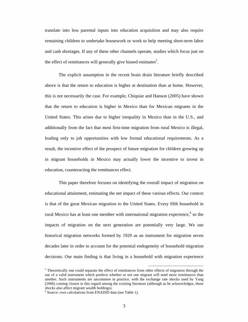
translate into less parental inputs into education acquisition and may also require

remaining children to undertake housework or work to help meeting short-term labor

and cash shortages. If any of these other channels operate, studies which focus just on

the effect of remittances will generally give biased estimates5.

The explicit assumption in the recent brain drain literature briefly described

above is that the return to education is higher at destination than at home. However,

this is not necessarily the case. For example, Chiquiar and Hanson (2005) have shown

that the return to education is higher in Mexico than for Mexican migrants in the

United States. This arises due to higher inequality in Mexico than in the U.S., and

additionally from the fact that most first-time migration from rural Mexico is illegal,

leading only to job opportunities with low formal educational requirements. As a

result, the incentive effect of the prospect of future migration for children growing up

in migrant households in Mexico may actually lower the incentive to invest in

education, counteracting the remittances effect.

This paper therefore focuses on identifying the overall impact of migration on

educational attainment, estimating the net impact of these various effects. Our context

is that of the great Mexican migration to the United States. Every fifth household in

rural Mexico has at least one member with international migration experience,6 so the

impacts of migration on the next generation are potentially very large. We use

historical migration networks formed by 1920 as an instrument for migration seven

decades later in order to account for the potential endogeneity of household migration

decisions. Our main finding is that living in a household with migration experience

5 Theoretically one could separate the effect of remittances from other effects of migration through the use of a valid instrument which predicts whether or not one migrant will send more remittances than another. Such instruments are uncommon in practice, with the exchange rate shocks used by Yang (2006) coming closest in this regard among the existing literature (although as he acknowledges, these shocks also affect migrant wealth holdings). 6 Source: own calculations from ENADID data (see Table 1).

4

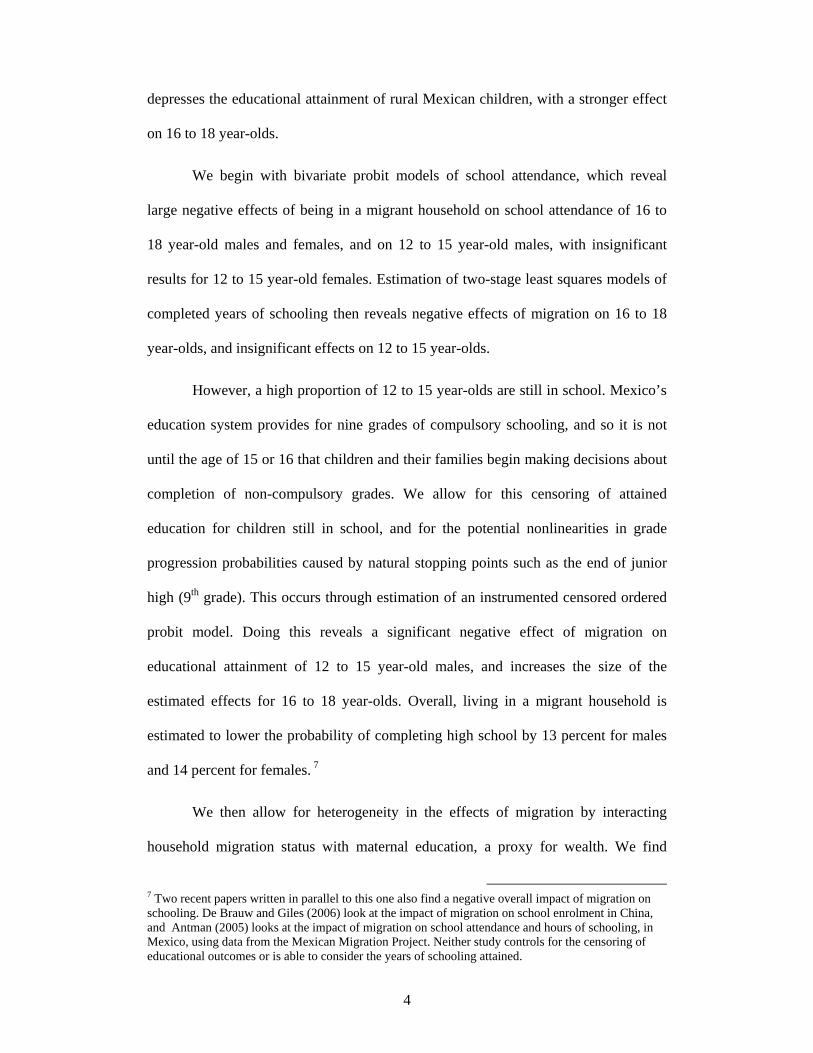
depresses the educational attainment of rural Mexican children, with a stronger effect

on 16 to 18 year-olds.

We begin with bivariate probit models of school attendance, which reveal

large negative effects of being in a migrant household on school attendance of 16 to

18 year-old males and females, and on 12 to 15 year-old males, with insignificant

results for 12 to 15 year-old females. Estimation of two-stage least squares models of

completed years of schooling then reveals negative effects of migration on 16 to 18

year-olds, and insignificant effects on 12 to 15 year-olds.

However, a high proportion of 12 to 15 year-olds are still in school. Mexico’s

education system provides for nine grades of compulsory schooling, and so it is not

until the age of 15 or 16 that children and their families begin making decisions about

completion of non-compulsory grades. We allow for this censoring of attained

education for children still in school, and for the potential nonlinearities in grade

progression probabilities caused by natural stopping points such as the end of junior

high (9th grade). This occurs through estimation of an instrumented censored ordered

probit model. Doing this reveals a significant negative effect of migration on

educational attainment of 12 to 15 year-old males, and increases the size of the

estimated effects for 16 to 18 year-olds. Overall, living in a migrant household is

estimated to lower the probability of completing high school by 13 percent for males

and 14 percent for females. 7

We then allow for heterogeneity in the effects of migration by interacting

household migration status with maternal education, a proxy for wealth. We find

7 Two recent papers written in parallel to this one also find a negative overall impact of migration on schooling. De Brauw and Giles (2006) look at the impact of migration on school enrolment in China, and Antman (2005) looks at the impact of migration on school attendance and hours of schooling, in Mexico, using data from the Mexican Migration Project. Neither study controls for the censoring of educational outcomes or is able to consider the years of schooling attained.

5

marginally significant evidence for less negative effects of migration on educational

attainment for children in poorer households, which is consistent with remittances

relaxing credit constraints. However, the overall effect of migration on education is

still negative for 16 to 18 year-olds, even in poor households. When we explore the

channels for this depressive effect of migration on schooling, we find the majority of

the effect can be explained by young males in migrant households themselves

migrating instead of attending school, and young females in migrant households

dropping out of school to engage in housework.

In related work, Hanson and Woodruff (2003) also estimate the overall impact

of migration on education in Mexico. They use the 2000 Mexican census, and look at

the impact on number of school grades completed of 10 to 15 year-olds. Their main

finding is that migration to the U.S. is associated with more years of completed

education for 13 to 15 year-old girls, but only for those whose mothers have three

years or less of education. We employ a large demographic survey instead of the

Census, allowing us to consider a broader measure of household migration

experience. We obtain an insignificant effect of migration on education for 12 to 15

year-olds girls with poorly educated mothers, and can not reject positive effects of

similar magnitudes to those they find. However, our work builds on their findings in

three important respects. Most fundamentally, we consider 16 to 18 year-olds, who

are at the age when migration for work starts to become a possibility, especially for

males, and who are also at the age when they may be entrusted with household

responsibilities which take the place of schooling. That is, this is precisely the age

range at which many of the other channels through which migration affects education

start to manifest themselves.

6

Secondly, Hanson and Woodruff (2003) note that school attendance is high

amongst their sample, with 82.5 percent of 10-15 year-olds attending school.

Nevertheless, they use two-stage least squares for estimation, which does not account

for this high rate of right-censoring. Once we account for censoring, insignificant

2SLS results for 12 to 15 year-old males become significant. Finally, the survey we

use enables examination of what children are doing when they are not in school,

enabling investigation of the channels through which migration is affecting schooling.

The remainder of this paper is organized as follows. Section 2 presents the

demographic survey data used for the empirical analysis and contrasts it to the 2000

Mexican Census. Section 3 discusses our identification strategy and other

econometric issues such as censoring and the presence of nonlinearities in education

decisions. Section 4 provides a broad theoretical framework that outlines how the

main effects of migration on the feasible and desired amounts of education balance

out at different wealth levels. The results on school attendance and education

attainments are presented in Section 5. Section 6 then asks what children in migrant

households are doing instead of going to school and Section 7 concludes.

2. Data

This paper uses data from the 1997 Encuesta Nacional de la Dinámica Demográfica

(ENADID) (National Survey of Demographic Dynamics) conducted by Mexico’s

national statistical agency (INEGI) in the last quarter of 1997.8 The ENADID is a

large nationally representative demographic survey, with approximately 2000

households surveyed in each state, resulting in a total sample of 73,412 households.

We restrict our analysis to rural communities, defined here to be municipalities which

are outside of cities of population 50,000 or more. Our main results are robust to

8 Survey methodology, summary tables, and questionnaires are contained in INEGI (1999).

7

lowering this threshold to cities with population below 15,000. Within these

communities we have a sample of 20,388 children aged 12 to 18 years, living in

12,980 households.

The key variables of interest are migration and schooling. The ENADID asks

several questions concerning migration, including whether household members have

ever been to the United States in search of work. This question is asked of all

household members who normally live in the household, even if they are temporarily

studying or working elsewhere. Additional questions ask whether any household

members have gone to live in another country in the past five years, capturing

migration for study or other non-work purposes in addition to work related migration.

We define a child as living in a migrant household if the household has a member

aged 19 and over who has ever been to the U.S. to work, or who has moved to the

U.S. in the last five years for any other reason. The migrant member or members may

have returned to Mexico or still be in the U.S. at the time of the survey.

Table 1 provides summary statistics for the key variables used in this study.

Twenty two percent of all households in our sample with a child aged 12 to 18 have

an adult member who has ever migrated to the U.S. Several recent studies of

migration and schooling in Mexico have used the 2000 Mexican Census (Hanson and

Woodruff, 2003; Lopez-Cordoba, 2005). The Mexican Census only asks about

migration within the last five years. The ENADID questions on migration within the

last five years are identically worded to the Census, and so for comparison we also

calculate the proportion of households with migrants according to the Census

definition. Table 1 shows that relying on the Census questions to define migrant

status understates the proportion of households with migrant experience by almost

fifty percent.

8

Examining migration within the last five years is likely not to be unduly

restrictive for certain types of analysis. However, there are number of reasons to

prefer looking at whether household members have ever migrated in examining the

impact of migration on education. Schooling is a cumulative process, with each year

building on the year before. Any impact of migration on schooling during the years of

primary education may therefore affect schooling six to ten years later. A portion of

this effect may be at the extensive margin: 10 percent of 12 year-olds in our sample

are not currently attending school, which makes it likely they will not be attending

school at age 18. There are also likely to be effects at the intensive margin, whereby

household resources and effort devoted to schooling during primary school affect the

ability of children to continue schooling in later years. In addition to these direct

effects through prior schooling, migration by household members six or more years

ago may still result in higher household wealth today, influencing the ability to pay

for schooling later on. Furthermore, schooling decisions may depend on the

expectation of migration in the future. This expectation will depend in part on

previous household migration experience, whether or not the migration episodes

occurred within the last five years. For these reasons we prefer the ENADID to the

Census for examining the effects of migration on education.

The ENADID asks migrants who have ever been to the U.S. for work a set of

additional questions about their migrant experience, including the number of trips

they have ever made, and whether they had legal documentation to work.

Approximately 50 percent of all migrants have made more than one trip, with a mean

of 2.8 trips per migrant. The vast majority of migrants in our sample had no legal

documentation to work, especially on their first trip. Over 91 percent of first-time

migrants who went to work in the U.S. had no legal documentation to do so. This is

9

important to note, as it indicates that the majority of Mexicans in our sample

contemplating migration are likely to end up working without documentation in the

United States. Kossoudji and Cobb-Clark (2002) find evidence from an amnesty

program that the returns to human capital are higher for legal workers than for illegal

workers in the United States. This corroborates our conjecture that migration lowers

the incentives to acquire education for prospective Mexican immigrants.9

Our main measure of education is based on years of schooling attained by

children and adults. Elementary education (grades 1 to 6) is compulsory in Mexico

and is normally provided to children aged 6 to 14. Lower secondary education (grades

7 to 9) became compulsory in 1993 and is generally given to children aged 12 to 16

years who have completed elementary education. This is followed by three years of

upper secondary schooling (grades 10 to 12) and higher studies. Despite education

being compulsory, there is still far from complete compliance and a lack of

infrastructure in some remote rural areas (SEP, 1999). Approximately half of all 15

year-olds with less than 9 years of attained schooling were not attending school in

1997. We focus our study on children aged 12 to 18, the ages at which children will

be receiving the majority of their post-primary education, and the age range at which

children start leaving school. 90 percent of 12 year-old males and 83 percent of 12

year-old females in our sample were attending school in 1997, compared to 51 and 47

percent of 15 year-old males and females, and 20 and 16 percent of 18 year-olds.

Figure 1 plots the proportion of females and males attending school by age

and the migrant status of their households, along with mean years of schooling

attained by age. The raw data show school attendance is higher in migrant households

among young children of five or six years, and similar in migrant and non-migrant

9 See also Rivera-Batiz (1999).

10

households in the early teenage years. However, school attendance drops among boys

in migrant households relative to non-migrant households from age 14 onward. The

result of this is that mean schooling levels attained for boys are very similar in

migrant and non-migrant households, while girls in migrant households have higher

mean schooling levels as they age than girls in non-migrant households. However,

these are unconditional differences, and do not take account of other differences

between migrant and non-migrant households which also affect schooling. We turn to

this issue next.

3. Empirical Methodology and Identification Strategy

3.1. Identification

The first challenge in estimating the causal impact of migration on education

outcomes is the possibility of unobserved characteristics of households which

influence their decision to migrate also playing a role in their schooling decisions. For

example, parents who care more strongly about the education of their children may

migrate in order to earn income that can be used to pay for schooling expenses, and

will also devote more attention and non-income resources to improving schooling

outcomes of their children. A simple comparison of migrants and non-migrants would

in this case overstate the education gains from migration. Alternatively, Hanson and

Woodruff (2003) note that negative labor market shocks experienced by parents may

both induce migration and require children to work instead of spending time in

school, leading to a spurious negative relationship between migration and years of

schooling. As such the direction of any selectivity bias is theoretically uncertain.

11

We therefore follow Woodruff and Zenteno (2007) and a number of

subsequent studies10 in using historic state-level migration rates as an instrument for

current migration stocks. In particular, we use the U.S. migration rate from 1924 for

the state in which the household is located, taken from Foerster (1925)11. Since this

instrument only varies at the state level, we cluster our standard errors at the state

level to allow for arbitrary correlation in the error structure of individuals within a

state.12 These historic rates can be argued to be the result of the pattern of arrival of

the railroad system in Mexico coupled with changes in U.S. demand conditions for

agricultural labor. As migration networks lower the cost of migration for future

migrants, they become self-perpetuating, and as a result, continue to influence the

migration decisions of households today.

Our identifying assumption is then that historic state migration rates do not

affect education outcomes over 70 years later, apart from their influence through

current migration. Instrumental variables estimation relies on this exogeneity

assumption, and so it is important to consider and counteract potential threats to its

validity. One potential threat is that historic levels of inequality and historic schooling

levels helped determine migration rates in response to the railroad expansion, and also

influence current levels of schooling due to intergenerational transmission of

schooling. To allow for this possibility we control for a number of historic variables at

around the same time period as our historic migration measure. The controls are the

proportion of rural households owning land by state in 1910 taken from McBride

(1923)13; and the number of schools per 1000 population by state in 1930, and male

10 Hanson and Woodruff (2003); McKenzie and Rapoport (2007); López-Córdoba (2005); and Hildebrandt and McKenzie (2005) all employ historic migration rates as instruments for current migration. 11 Thanks to Chris Woodruff for supplying these historic rates. 12 Mexico has 31 states and a federal district. 13 Land ownership data were kindly provided by Ernesto López-Córdoba.

12

and female school attendance for 6 to 10 year-olds by state for 1930, both taken from

DGE (1941).

A second possible threat to validity is that the development of the railroads in

certain states and communities ushered in the subsequent development of other

infrastructure, such as school facilities, and led to changes in the income distribution

which themselves influenced the incentives and ability to invest in schooling. We

include the following state-level controls for this possibility, all calculated from the

public use sample of the 1960 Mexican Census: the Gini of household income, the

Gini of years of schooling accumulated for males and females aged 15-20, and the

average levels of years of schooling accumulated for males and females aged 15-20.

Spearman rank-order correlation tests do indeed indicate some significant correlations

between the 1924 migration rates and some of these controls: states with higher

historic migration rates had higher average rates of schooling and lower inequality in

schooling in 1960. This might represent the influence of migration over the 1924-60

period, or the effects of concomitant trends, and so we prefer to include these 1960

education inequality and levels as controls. Even after controlling for these variables,

historic migration rates remain a powerful predictor of current community migration

prevalence, with a first-stage F-statistic of 28.

A final threat to the validity of this instrument is the possibility that the

historic community migration network has a direct effect on educational attainment

through changing the incentives to acquire education. We argue that the incentive

effects should be much stronger if children have a household member who has

previously migrated than if they merely have someone in their community who has

migrated, so that the direct effect of the community network is likely to be second-

order in the education decision. As a check on this assumption, we split states into

13

those above and below the median migration rate in 1924, and then regress years of

schooling on a dummy variable for being in a high migration state for children in non-

migrant households. Table 2 shows the effect of the community network is

insignificant for three out of the four groups, and has a small positive effect on school

attainment of 12 to 15 year-old females. This provides us with further confidence in

our instrument and suggests that a finding of migration lowering education rates is not

a result of the community network directly lowering education rates.

It is also worth discussing why we do not follow Hanson and Woodruff (2003)

in including state fixed effects and using the interaction between historic migration

rates and maternal characteristics as the instrument. The most important reason we do

not do this is that we do not believe this solves the identification problem. As

discussed, a possible concern with our identification strategy is that there are

unobserved state-level characteristics, such as schooling infrastructure, which are

correlated with historic migration rates and which also affect education outcomes.

Including state fixed effects and using the interaction between historic migration rates

and mother’s education as the instrument then requires assuming that the effect of

such variables such as schooling infrastructure on child education does not vary with

mother’s education. We prefer to directly control for as many of these state-level

variables as we can, rather than assuming that they exist but don’t have differing

effects by maternal characteristic.

There are two further reasons we do not include state-level fixed effects and

use the interaction between historic migration rates and maternal characteristics as an

instrument. The first is that, with the ENADID sample size, these instruments are very

weak. Using the full set of interactions employed by Hanson and Woodruff (2003),

we obtain first-stage F-statistic ranging from 0.80 to 2.02, with over 10 interactions

14

used. Using a more parsimonious specification which includes only mother’s

education, mother’s education squared, and mother’s age as interactions still results in

first-stage F-statistics ranging from 0.78 to 4. The 2SLS coefficients we get in this

case are all negative in sign, but insignificant, reflecting the weak instruments

drawing the estimates back towards OLS.

Secondly, it is well-known that when there are heterogeneous treatment

effects, instrumental variables will identify a local-average treatment effect (LATE).

In our case, this will be the impact of migrating on households which would migrate

when they have a large network, and which wouldn’t migrate when they have a small

network. As shown in McKenzie and Woodruff (2007), these marginal households are

typically drawn from the lower end of the wealth distribution, and are households

which can’t meet the costs of migrating when networks are small. Since these are

poorer, more marginal migrants, they seem an appropriate subgroup of interest for

learning about the impact of migration on their children’s education. In contrast, when

multiple interactions between maternal characteristics and historic migration rates are

used as instruments, the instrumental variables estimator will give a local-average

treatment effect than is more difficult to interpret and less likely to be of direct policy

interest, being an average of different local-effects.

3.2. Estimation techniques

The first outcome of interest that we study is whether children are currently attending

school. As this is a binary outcome, we use maximum-likelihood to estimate a

bivariate probit model, following Newey (1987), which we will follow common

practice in referring to as the IV-Probit model.14 The marginal effects of this model

will then be compared to marginal effects from standard probit estimation. However,

14 Estimation was carried out using the IVProbit command in STATA version 9.

15

current school attendance does not allow for possible delays in starting schooling,

catch-up and grade repetition. As seen in Figure 1, it appears that children in migrant

households are slightly more likely to start school at age 5 than children in non-

migrant households. Therefore greater attendance in non-migrant households at older

ages may just be the result of these late starters catching up.

Instead of school attendance, we therefore focus most of our attention on

educational attainment, measured by the grade-years of schooling attained by

children. Following Hanson and Woodruff (2003) we begin with two-stage least

squares (2SLS) of the following equation:

Schoolingi = α+β*Migranti+δ’Xi +εi (1),

where Schoolingi is the years of schooling attained by child i, Migranti is a dummy

variable taking the value one if a household has a migrant member and zero

otherwise, and Xi is a set of individual and community controls.

However, there are several features of education data that render OLS and

2SLS analysis inappropriate. Ideally one would like to observe the final level of

schooling completed by individuals and relate it to the migrant status of the household

in which they grew up. Here we face the problem that while schooling is complete for

adults, we have no information on the households in which they lived during their

childhood, or on the migration status of their parents. We must therefore restrict our

sample to children of school age. However, while we have information on the

migration status of the households in which these children are living, many of them

are still attending school and so we do not observe their completed level of schooling.

The data are thus right-censored for children who are attending school. OLS

and 2SLS estimation ignores this censoring, treating the educational attainment of

16

children still in school as identical to those who have finished schooling. This results

in biased estimates of the impact of migration on final schooling attainment.

Censoring is likely to be especially important for schooling outcomes of 12 to 15

year-olds, since many in this age group will not have finished schooling.

A second issue is that OLS and 2SLS assume a continuous distribution for the

dependent variable, years of schooling attained. However, as seen in Figure 2, the

observed schooling distribution is characterized by large spikes at 6 years and 9 years,

representing the completion of primary and lower secondary school. As noted in the

education literature (see e.g., Glick and Sahn, 2000), grade attainment is the outcome

of a series of ordered discrete choices. The choice to continue onto junior secondary

school or onto high school for one year is thus likely to be different from the choice to

continue for an extra year once one has started junior high or high school.

As a result of these features of education grade data, King and Lillard (1987)

and subsequent studies in the economics of education literature (e.g. Glick and Sahn

(2000), Holmes (2003), Maitra (2003)) have adopted a censored ordered probit

framework when examining the impact of household characteristics on schooling. In

this framework, an individual’s desired latent propensity for schooling, yi is

determined by a linear relationship analogous to equation (1):

yi = α+β*Migranti+δ’Xi +εi (2)

However, yi is unobserved. For individuals who have finished their schooling,

we observe schooling level S if the value of yi falls between two cut-off points,

corresponding to grades S and S+1:

1+≤< SiS y μμ (3)

17

For individuals with no schooling, we only know that the index falls below the lowest

threshold, normalized to zero, and for individuals with the maximum level of

schooling, we know only that yi ≥ μmax. We classify education grade attainment into

seven ordered categories for the purposes of this analysis: no schooling, 1 to 5 years,

6 years (complete primary), 7 to 8 years, 9 years (completed junior high), 10 to 11

years, and 12 and above years (completed high school). Assuming normality of the

error terms, εi, one can then write down the likelihood function, and via this ordered

probit model, estimate these cutoff points along with the coefficients of interest (see

Greene, 2000). For children who are still in school, we know that they will attain at

least their current grade, and hence that for an individual currently in school with J

grades of schooling attained, yi ≥ μJ. One can therefore modify the likelihood function

to allow for this censoring, and estimate the censored ordered probit model via

maximum-likelihood.15

To allow for the potential endogeneity of household migration status within

the ordered probit and censored ordered probit model we follow the methodology of

Rivers and Vuong (1988). In the first stage, a household migrant status is regressed on

the instrument and exogenous regressors. The fitted values and residuals from this

first stage are then both included in the censored ordered probit model estimated in

the second stage.16 We will refer to the estimates from this process as IV-Ordered

Probit and IV-Censored Ordered Probit estimates.

15 See Appendix A of Glick and Sahn (2000) for specification of the likelihood function. Estimation was carried by programming the likelihood in STATA version 9. 16 Such an approach is also carried out by Maitra (2003).

18

4. Theoretical framework

We now turn to an examination of the theoretical impact of migration on the

schooling of children. Let ri,s denote the present discounted value of the additional

returns to child i of completing schooling year s, ci,s denote the additional financial

costs of the child completing this additional year of schooling, and ki,s denote the

additional non-financial costs of the child completing this additional schooling year,

such as foregone income and the disutility of school effort. Costs are realized at the

moment of schooling whereas returns are not realized until the future. Financial costs

of schooling must therefore be met out of the household’s current resources. The

household’s schooling decision is then to choose s ∈{0,1,2,…,N} to maximize the net

present discounted value of schooling, subject to the condition that total financial

schooling costs must be met out of current household resources net of subsistence

needs, Ai. That is,

{ }( ) ∑∑

==∈≤−−=

s

jiji

s

jjijiji

Nsi Actskcrs

1,

1,,,

,...,2,1,0

* ..maxarg (4)

Let siU

denote the unconstrained optimal level of education for child i, which

occurs when the financing constraint does not bind. We expect this to be weakly

increasing in mother’s education and household resources due to the possibility of

more educated mothers lowering the disutility and non-financial costs of schooling by

placing higher emphasis on education, helping with schoolwork, and perhaps due to a

genetic ability component. The returns to schooling may also be higher for richer

households due to peer effects and the ability to enter occupations with high start-up

costs. Denote by siP the maximum possible years of schooling the household can

afford under its budget constraint. This is clearly increasing in wealth, and is likely to

19

be increasing in maternal education since household resources are likely to be

correlated with mother’s schooling. Then:

( )Pi

Uii sss ,min* = (5)

Figure 3 then illustrates the relationship between si* and household wealth levels or

maternal education. Child schooling is predicted to increase with household resources,

both due to relaxing of credit constraints and to the possible higher desired levels of

education for children in richer households with more educated mothers.

Now consider the potential impacts of migration on a household’s optimal

education. Remittances and potentially higher earnings after migration (such as from

entrepreneurship, see Woodruff and Zenteno, 2007, or farm investments, see Taylor

and Wyatt, 1996) increase the value of household resources Ai, increasing the

maximum years of schooling the household can afford, siP. The relaxation of credit-

constraints allows households to move to or towards their unconstrained optimal level

of education, resulting in higher education for their children. In contrast, if credit

constraints are not binding, then remittances will have no effect on their schooling.

In addition to remittances, migration can have a number of other effects on

child schooling. Hanson and Woodruff (2003) note that one potential negative effect

is that migration may disrupt household structure, removing children from the

presence of guardians and role models, and require older children to take on

additional household responsibilities. In our model this can be thought of as

increasing the non-financial costs of schooling, ki,s, leading households to lower siU,

their unconstrained level of education.

A further effect which we wish to consider is the possibility that due to

information and network effects, having a migrant parent increases the likelihood that

20

the children themselves will become migrants. This may have an immediate

substitution effect, whereby as a result of the opportunity cost of staying in school

increasing due to higher potential earnings abroad, children drop out of school in

order to migrate to work. Again this can be viewed as increasing ki,s, leading

households to lower siU.

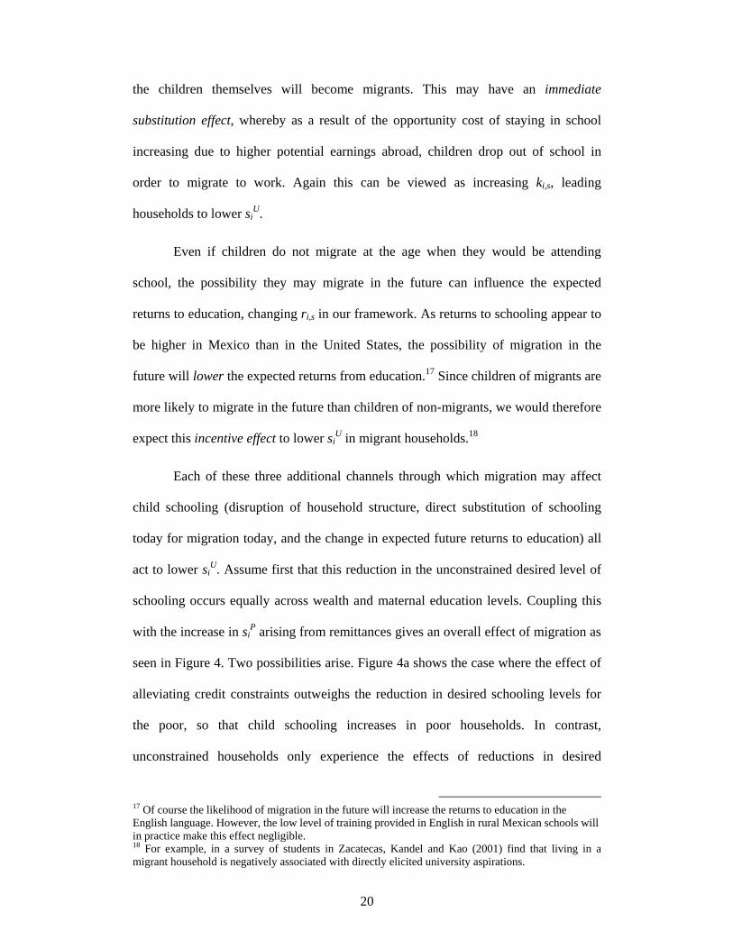
Even if children do not migrate at the age when they would be attending

school, the possibility they may migrate in the future can influence the expected

returns to education, changing ri,s in our framework. As returns to schooling appear to

be higher in Mexico than in the United States, the possibility of migration in the

future will lower the expected returns from education.17 Since children of migrants are

more likely to migrate in the future than children of non-migrants, we would therefore

expect this incentive effect to lower siU in migrant households.18

Each of these three additional channels through which migration may affect

child schooling (disruption of household structure, direct substitution of schooling

today for migration today, and the change in expected future returns to education) all

act to lower siU. Assume first that this reduction in the unconstrained desired level of

schooling occurs equally across wealth and maternal education levels. Coupling this

with the increase in siP arising from remittances gives an overall effect of migration as

seen in Figure 4. Two possibilities arise. Figure 4a shows the case where the effect of

alleviating credit constraints outweighs the reduction in desired schooling levels for

the poor, so that child schooling increases in poor households. In contrast,

unconstrained households only experience the effects of reductions in desired

17 Of course the likelihood of migration in the future will increase the returns to education in the English language. However, the low level of training provided in English in rural Mexican schools will in practice make this effect negligible. 18 For example, in a survey of students in Zacatecas, Kandel and Kao (2001) find that living in a migrant household is negatively associated with directly elicited university aspirations.

21

schooling, and so schooling falls. Figure 4b shows the case in which the fall in desired

schooling is sufficiently large that no household would have been credit-constrained,

even in the absence of remittances. In this case, schooling falls for all wealth levels

after migration, but still should fall by more for richer households.

Nevertheless, under some circumstances one might anticipate seeing more of a

reduction in schooling among poorer households following migration, and a

corresponding increase in education inequality. Figure 4c outlines one such scenario.

Basic education is provided free by the state along with free textbooks (SEP, 1999).

Along with a number of targeted programs towards the poor, it is likely that even the

poorest Mexican households have sufficient household resources to afford some years

of post-primary schooling. It is therefore possible that desired schooling levels lie

below possible schooling. Migration may then lower siU by more for poorer

households than for richer households. Therefore in addition to the overall impact of

migration on education being uncertain, it is also uncertain as to how the size of the

effect will vary with wealth.

5. Results

5.1. School Attendance

Table 3 presents the probit and IV-probit estimates of the impact of being in a migrant

household on school attendance. The probit results show a significant, but small,

negative impact of being in a migrant household on school attendance of boys, and an

insignificant effect on school attendance of girls. Once we instrument for migration

however, these effects become larger, and being in a migrant household is estimated

to significantly lower the probability of attending school by 16 percentage points for

12 to 15 year-old males, 21 percentage points for 16 to 18 year-old males, and 20

22

percentage points for 16 to 18 year-old females. The coefficient on migration for

females aged 12 to 15 is also negative, but is insignificant. All specifications also

show a strong positive effect of mother’s years of education on school attendance, and

that children in areas which have historically had more schools are currently more

likely to attend school.

5.2. Years of Schooling Attained

Tables 4 to 7 present the results of estimating the impact of being in a migrant

household on grade years of schooling attained for each sex-age group. In each table,

Columns 1 and 2 first present the OLS and 2SLS estimates of equation (1). Column 3

gives the ordered probit estimates, and Column 4 gives the iv-ordered probit

estimates. Column 5 gives the censored ordered probit estimates, while column 6

adjusts these for endogeneity of migration.

The OLS results show a positive overall association of migration with attained

years of schooling, which is significant for females and for males aged 12 to 15.

However, once we control for the endogeneity of migration, the 2SLS results all show

a negative impact for migration on schooling, with this effect being significant for 16

to 18 year-old males and females. Comparison of the OLS and 2SLS results therefore

suggests that children in migrant households have unobserved characteristics which

make them more likely to receive schooling than observationally similar children in

non-migrant households. This would be consistent with migration of parents who care

a lot about the education of their children.

The iv-ordered probit and iv-censored order probit results show the

importance of allowing for these more complex specifications. The negative impact of

migration on education of males aged 12 to 15 is significant in these two

23

specifications, compared to the insignificant 2SLS specification. The significance

level also increases for the negative impact on males and females aged 16 to 18.

Comparison of the iv-ordered probit and iv-censored ordered probit results shows a

stronger negative impact of migration after allowing for censoring, with this

difference greater amongst 12 to 15 year-olds than amongst 16 to 18 year-olds. This

concurs with our a priori view that censoring was particularly likely to be a problem

for estimation of schooling at younger ages. The impact of migration on schooling is

still insignificant for females aged 12 to 15 after allowing for censoring and

differential schooling level effects.

The size of the effects can not be easily seen from the coefficients in Tables 4

to 7. Interpretation of the coefficients of an ordered probit model is complicated by

the fact that the direction of the effect is only unambiguous for the lowest and highest

category (see Greene, 2000, p. 878). As a result, we calculate the marginal effect of a

change in household migrant status on the probability of having schooling of each one

of our seven categories. Marginal effects can be further complicated in a censored

model, since a change in a variable of interest will affect both schooling attained at

the time of observation, and the probability of the observation being censored by the

child continuing to attend school. We report marginal effects for the change in the

latent index, which captures both of these effects, and therefore provides an estimate

of the impact of migrant status on final schooling attainment.

Table 8 reports the marginal coefficients from the iv-ordered probit and iv-

censored ordered probit models. These effects demonstrate that living in a migrant

household has different effects at different levels of schooling, and it is not the case

that the effects are linear. For example, for 12 to 15 year-old males, the instrumented

censored order probit model shows that living in a migrant household lowers the

24

probability of having 9 years of completed education by 22.5 percent, and lowers the

probability of having 10 or 11 years of education (or more) by 12 percent. These

effects are substantially larger than in the ordered probit model which does not allow

for censoring, reflecting the fact that many 12 to 15 year-olds are still in school.

Similarly for 15 to 18 year-old males and females, allowing for censoring shows a

much larger effect of migration on lowering the probability of completing 12 years or

more education. Overall these marginal effects show migration having very little

effect on the probability of completing 7 to 8 years of education, while lowering the

probabilities of receiving more years than this, and increasing the probability of

receiving less years than this.

5.3. Allowing for heterogeneous effects

As discussed in Section 4, the impact of migration on education may possibly vary

with household wealth, since households with lower wealth may be more likely to be

liquidity constrained when making their education decisions. In such cases, the

remittance effect of migration is likely to relax these liquidity constraints and

therefore potentially increase education, or at least not reduce it as much as one sees

for those with higher wealth levels. Unfortunately the ENADID contains only limited

information on household wealth, in the form of current asset indicators, which are

themselves affected by a household’s migration decision. We therefore instead use

maternal education as a proxy for household wealth: mother’s years of schooling has

a 0.46 correlation with an asset index formed as the first principal component of a

number of asset indicators in our sample.

Table 9 then reports the results of 2SLS estimation of the impact of living in a

migrant household on child schooling, interacted with mother’s education. We

employ two methods of carrying out this interaction. The first is a straight interaction

25

with the number of years of schooling. Secondly, we concentrate on the poorest

segment by interacting with whether or not the child’s mother has two years or less of

education. We use 2SLS rather than the censored ordered probit for ease of

interpreting the coefficients on the interactions, and because the likelihood functions

did not always converge in ordered probit estimation with interactions.

Table 9 offers only limited evidence for heterogeneous effects of migration on

child’s schooling. The interaction effect with total years of schooling of the mother is

always negative, indicating that children in households which are likely to be richer

have even more of a negative impact from migration. However, none of these

interaction terms are significant. When we interact with the mother having two years

or less of schooling, we find positive interaction effects, showing that children in

poorer households are less likely to face a reduction in years of schooling from

migration. These interaction effects are significant at the 10 percent level for females

16 to 18 and at the 11 percent level for females 12 to 15. For the 12 to 15 year

females, the size of the coefficient is almost enough to take the overall effect of

migration for children with less-educated mothers to zero. Moreover, the standard

error is such that we can’t reject a positive effect for this group of magnitudes similar

to the 0.7 years estimated by Hanson and Woodruff (2003). However, for the 16 to 18

year-old females, the overall effect of migration is still negative, just less negative

than for females of this age with more educated mothers.

6. What are they doing instead of school?

The above analysis has found that children in migrant households are less likely to be

attending school and complete less total years of schooling than children in non-

migrant households. In this section we explore what these children are doing instead

of schooling. It is possible that the absence of a migrant parent may require the child

26

to undertake tasks normally carried out by that migrant, such as working in a family

business or doing housework. Since it can take a while for migrants to start earning

money and remitting, children may also need to work to cover short-term household

liquidity constraints.19 Any of these activities are also consistent with the child (or the

parents) no longer valuing schooling due to future migration plans. Finally we can

also examine whether or not the child has migrated during this age range where they

could be still engaged in schooling.

Table 10 reports the percentage of 12 to 18 year-olds by sub-age group and

gender who are in school, working, working and not in school, migrated, doing

housework, and working in family businesses. Children in migrant households are

more likely to have migrated themselves than children in non-migrant households,

especially among males. 3.4 percent of 12 to 15 year-old males and 8.2 percent of 16

to 18 year-old males with older migrant members in the household have themselves

migrated, compared to only 0.2 percent of males in non-migrant households. Males

also are more likely to be working, especially as unpaid workers in family businesses,

if they are in migrant households. In contrast, female youth in migrant households are

not that likely to migrate themselves, and instead are more likely to be engaged in

housework than female youth in non-migrant households.

In Table 11 we examine whether the differences observed in Table 10 are

significant once we control for observable differences between children in migrant

and non-migrant households and control for the endogeneity of migration. We present

probit results for whether or not the child has migrated, since the historic migrant

19 The ENADID asks whether or not you have worked in the past week, regardless of whether or not you are also attending school, which we define as working. Another possible activity in the last week for individuals who were not students and who were not working was doing housework. Among the individuals who are working, we also look more closely to see whether or not they are working as unpaid workers in a family enterprise, defined as unpaid family workers.

27

network instrument is clearly not excludable from this model. For the other outcomes,

we again instrument living in a migrant household with historic migration rates, using

IV-probit models. The results show children living in migrant households to be

significantly more likely to migrate themselves than observationally similar children

living in non-migrant households. This effect is largest for 16 to 18 year-old males,

who are 7.3 percent more likely to migrate when living in migrant households.

Migrant and non-migrant males do not exhibit significantly different probabilities of

working or engaging in housework, and the higher likelihood of working in family

businesses observed for males in migrant households in Table 10 is not significant.

Among females, we see a strong significant effect of living in a migrant household on

doing housework.

How much then do these other activities explain the lower school participation

of children in migrant households? Comparing the marginal effects of migration on

school attendance in Table 3 to those on participation in these other activities in Table

11 shows that current migration can more than account for the lower likelihood of

school participation for 16 to 18 year-old males, and can account for 60 percent of the

lower likelihood of school participation for 12 to 15 year-old males. For 12 to 15

year-old females, there was no significant effect of migration on school attendance,

but housework can account for the size of the point estimate. For 16 to 18 year-old

females, the increase in housework as the main activity more than accounts for the

decrease in schooling, with a decrease in non-school work also needed to account for

the large increase in housework.

One possible concern with the finding that the male drop in schooling is

driven by higher likelihoods of migration for male youths in migrant households

could be that these youths are migrating in order to continue their education in the

28

United States. Data on all schooling levels attained (whether in Mexico or in the U.S.)

are recorded and used in our analysis for seasonal migrants who have returned to

Mexico, or who remain as part of the family. Furthermore, the ENADID specifically

asks whether individuals have migrated to the U.S. in order to work, or to seek work,

in addition to asking separately whether they have lived in the U.S. in the last 5 years.

The data shows that 81 percent of 16-18 year old males going to the U.S. went there

to work or in search of work. It is likely that some of the remainder were also not in

school, even if they didn’t go specifically for work. Thus it appears that the migration

of male youth from rural Mexico during this period is for work, not schooling, and

that this explains a large part of the lower schooling attainment of male Mexican

youth.

7. Conclusion

This paper examined the overall impact of migration on educational attainment in

rural Mexico. This impact is the sum of three main effects: the effect of remittances

on the feasible amount of education investment, which is likely to be positive where

liquidity constraints are binding; the effect of having parents absent from the

household as a result of migration, which may translate into less parental inputs into

education acquisition and maybe into more house and farm work by remaining

household members, including children; and the effect of migration prospects on the

desired amount of education, which is likely to be negative, as we argued, in the face

of lower returns to schooling in the U.S. than in Mexico, especially in a context of

illegal immigration.

Our results are in line with these predictions. Using historical migration rates

by state to instrument for current migration, we find evidence of a significant negative

effect migration on schooling attendance and attainments of 12 to 18 year-old boys

29

and of 16 to 18 year-old girls. IV-Censored Ordered Probit results show that living in

a migrant household lowers the chances of boys completing junior high school (by 22

percent) and of boys and girls completing high school (by 13 to 15 percent). This is

consistent with migration increasing the opportunity cost, and lowering the expected

return to education. However, the negative effect of migration on schooling is

somewhat mitigated for younger girls with low educated mothers, which is consistent

with remittances allowing to relax credit constraints on education investment at the

lower end of the wealth and income distribution.

We also examine what children are doing instead of going to school and find

that living in a migrant household significantly increases the chances of boys

migrating themselves at all school ages and of older (16 to 18 year-old) girls doing

housework. Comparison of the marginal effects of migration on school attendance and

on participation to other activities shows that the observed decrease in schooling of 16

to 18 year-olds is more than accounted for by current migration of boys and increases

in housework for girls. This is at an age where work is also an important form of

human capital accumulation, so it appears that Mexican females in migrant

households are losing out on both schooling and work.

To the extent that this reduction in education is a conscious choice of

individuals in the face of better opportunities abroad, it should be less of a policy

concern than a restriction on schooling due to liquidity constraints. However, given

the large literature on positive externalities of education, there may still be some

concern at this effect of potential migration on schooling incentives. One possible

policy solution would be to take measures to increase the return to schooling in the

U.S., which is likely to occur if migrants have better access to legal jobs.

30

7. References Acosta, Pablo (2006) “Labor supply, school attendance, and remittances from international

migration: the case of El Salvador”, World Bank Policy Research Working Paper No. 3903.

Antman, Francisca (2005) “The Intergenerational Effects of Paternal Migration on Schooling”, Mimeo. Stanford University.

Beine, Michel, Frederic Docquier and Hillel Rapoport (2007): Brain drain and human capital formation in developing countries: winners and losers, Economic Journal, forthcoming.

Chiquiar, Daniel and Gordon H. Hanson (2005): International migration, self-selection, and the distribution of wages: Evidence from Mexico and the United States, Journal of Political Economy, 113, 2: 239-81.

Commander, Simon, Maria Kangasniemi and Allan L. Winters (2004): The brain drain: curse or boon? A survey of the literature, in R. Badlwin and L.A. Winters, eds.: Challenges to Globalization, The University of Chicago Press, Chapter 7.

Cox Edwards, A. and M. Ureta (2003): Internation migration, remittances and schooling: evidence from El Salvador, Journal of Development Economics, 72, 2: 429-61.

de Brauw, Alan and John Giles (2006) “Migrant Opportunity and the Educational Attainment of Youth in Rural China”, IZA Discussion Paper No 2326, September 2006.

Dirección General de Estadística (DGE) (1941) Anuario Estadístico de los Estados Unidos Mexicanos 1939. Secretaría de la Economía Nacional, DGE: Mexico City.

Foerster, Robert F. (1925) The Racial Problems Involved in Immigration from Latin America and the West Indies to the United States. Washington D.C.: The United States Department of Labor.

Glick, Peter and David E. Sahn (2000) “Schooling of girls and boys in a West African country: the effects of parental education, income, and household structure”, Economics of Education Review 19: 63-87.

Greene, William H. (2000) Econometric Analysis: Fourth Edition, Prentice-Hall: Upper Saddle River, New Jersey.

Hanson, Gordon H. and Christopher Woodruff (2003): Emigration and educational attainment in Mexico, Mimeo., University of California at San Diego.

Hildebrandt, Nicole and David J. McKenzie (2005) “The Effects of Migration on Child health in Mexico”, Economia 6(1): 257-89.

Holmes, Jessica (2003) “Measuring the determinants of school completion in Pakistan: analysis of censoring and selection bias”, Economics of Education Review 22: 249-64.

Instituto Nacional de Estadística, Geografía e Informática (INEGI) (1999). ENADID: Encuesta Nacional de la Dínamica Demográfica 1997. INEGI: Aguascalientes.

Kandel, William and Grace Kao (2001): The impact of temporary labor migration on Mexican children’s educational aspirations and performance, International Migration Review, 35, 4: 1205-31.

King, Elizabeth M. and Lee A. Lillard (1987) “Education policy and schooling attainment in Malaysia and the Philippines”, Economics of Education Review 6(2): 167-81.

Kossoudji, Sherrie A. and Deborah A. Cobb-Clark (2002) “Coming out of the shadows: learning about legal status and wages from the legalized population”, Journal of Labor Economics 20(3): 598-628.

López-Córdoba, Ernesto (2005) “Globalization, Migration, and Development: The Role of Mexican Migrant Remittances”, Economia 6(1): 217-56.

Maitra, Pushkar (2003) “Schooling and Educational Attainment: Evidence from Bangladesh”, Education Economics 11(2): 129-53.

McBride, George M. (1923) The Land Systems of Mexico. New York: American Geographical Society.

McKenzie, David (2005): Beyond remittances: the effects of migration on Mexican households, in Caglar Ozden and Maurice Schiff, eds.: International migration, remittances and the brain drain, McMillan and Palgrave. Chapter 4, pp. 123-47.

31

McKenzie, David and Hillel Rapoport (2007): Network effects and the dynamics of migration and inequality: theory and evidence from Mexico”, Journal of Development Economics 84(1): 1-24.

Newey, Whitney K. 1987. “Efficient Estimation of Limited Dependent Variable Models with Endogenous Explanatory Variables.” The Journal of Econometrics November 36(3): 231-250.

Rapoport, Hillel and Frederic Docquier (2006): The Economics of Migrants’ Remittances, in S.-C. Kolm and J. Mercier Ythier, eds.: Handbook of the Economics of Giving, Altruism and Reciprocity, Amsterdam: North Holland. Vol. 2, Chap. 17, pp. 1135-98.

Rivera-Batiz, Francisco (1999) “Undocumented workers in the labor market: An analysis of the earnings of legal and illegal Mexican immigrants in the United States”, Journal of Population Economics 12:91-116.

Rivers, Douglas and Quang H. Vuong (1988) “Limited Information Estimators and Exogeneity Tests for Simultaneous Probit Models”, Journal of Econometrics 39: 347-66.

Secretaría de Educación Pública (SEP) (1999) Profile of Education in Mexico. Ministry of Public Education, http://www.sep.gob.mx.

Taylor, J. Edward and T.J. Wyatt (1996) “The Shadow Value of Migrant Remittances, Income and Inequality in a Household-farm Economy”, Journal of Development Studies 32(6): 899-912.

Woodruff, Christopher, and Rene M. Zenteno (2007): Remittances and micro-enterprises in Mexico”, Journal of Development Economics 82(2): 509-28.

World Bank (2005) Global Economic Prospects 2006: Economic Implications of Remittances and Migration, The World Bank, Washington D.C.

Yang, Dean (2006) “International Migration, Human Capital, and Entrepreneurship: Evidence from Philippine Migrants’ Exchange Rate Shocks”, Economic Journal, forthcoming.

0.2

.4.6

.81

5 10 15 20Age

Migrant Household Non-migrant Household

School Attendance - Boys

0.2

.4.6

.81

5 10 15 20Age


School Attendance - Girls

02

46

8

5 10 15 20Age


Mean Years of Schooling - Boys

02

46

85 10 15 20

Age


Mean Years of Schooling - Girls

Figure 1: School attendance and attainment by age and sex

32

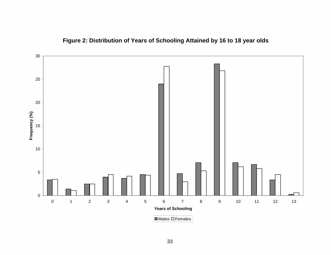
Figure 2: Distribution of Years of Schooling Attained by 16 to 18 year olds

0

5

10

15

20

25

30

0 1 2 3 4 5 6 7 8 9 10 11 12 13

Years of Schooling

Freq

uenc

y (%

)

Males Females

33

FIGURE 3: REMITTANCE EFFECT ON CHILD SCHOOLING

Remittances shift the possible schooling line upwards, increasing education for poorer households. Bold line shows the new education choice, bold dashed line shows the old education choice.

FIGURE 4: OVERALL EFFECT OF MIGRATION ON CHILD SCHOOLING

Figure 4a: Equal but small reduction in unconstrained schooling

Bold dotted line shows the original schooling decision, bold solid line shows the new schooling decision after migration.

Household Wealth

Education sP (old)

su

sP (new)

Household Wealth

Education sP (old)

su (old)

sP (new)

su (new)

34

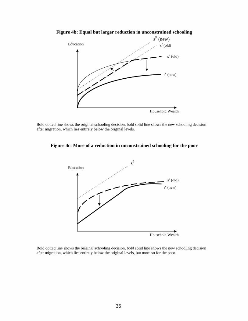
Figure 4b: Equal but larger reduction in unconstrained schooling

Bold dotted line shows the original schooling decision, bold solid line shows the new schooling decision after migration, which lies entirely below the original levels.

Figure 4c: More of a reduction in unconstrained schooling for the poor

Bold dotted line shows the original schooling decision, bold solid line shows the new schooling decision after migration, which lies entirely below the original levels, but more so for the poor.

Household Wealth

Education sP (old)

su (old)

su (new)

Household Wealth

Education

su (old)

su (new)

sP

sP (new)

35

TABLE 1: SUMMARY STATISTICS OF KEY VARIABLES

Number ofObservations Mean Std. Dev. Mean Std. Dev. Mean Std. Dev.

Household Variables (for households with a child aged 12 to 18)Proportion of Households with a migrant 12980 0.22 1 0Proportion of Households with a migrant by census definition 12980 0.13 0.60 0.002Proportion receiving remittances1 12301 0.06 0.22 0.02Percentage share of income from remittances1 12301 3.83 16.79 14.91 30.87 0.80 7.43Individual VariablesYears of Schooling of Mother for children aged 12 to 18 20388 3.32 3.20 3.47 2.98 3.28 3.27Years of Schooling of Males 12 to 15 6537 5.79 2.02 5.94 1.82 5.74 2.08Years of Schooling of Males 16 to 18 4159 7.10 2.85 7.10 2.73 7.10 2.88Years of Schooling of Females 12 to 15 6196 5.92 2.05 6.23 1.79 5.83 2.11Years of Schooling of Females 16 to 18 3489 7.32 2.87 7.52 2.58 7.26 2.96State level variablesState migration rate in 1924 20388 0.006 0.008 0.011 0.008 0.004 0.007Percentage of rural households owning land in 1910 20388 2.283 1.705 2.698 1.514 2.159 1.739Male School Attendance in 1930 (% of 6 to 10 year olds) 20388 39.39 9.00 39.902 8.153 39.242 9.226Female School Attendance in 1930 (% of 6 to 10 year olds) 20388 36.84 10.00 38.944 9.264 36.211 10.121Gini of Household Income in 1960 20388 0.783 0.069 0.778 0.068 0.784 0.069Number of Schools per 1000 population in 1930 20388 1.100 0.319 0.993 0.305 1.131 0.315Gini of Years of Schooling for Males 15-20 in 1960 20388 0.554 0.080 0.551 0.087 0.555 0.078Gini of Years of Schooling for Females 15-20 in 1960 20388 0.573 0.099 0.556 0.100 0.578 0.098Average Male Years of Schooling in 1960 20388 2.614 0.638 2.671 0.647 2.597 0.635Average Female Years of Schooling in 1960 20388 2.437 0.745 2.561 0.756 2.400 0.738

Source: own calculation from ENADID 1997 communities with population <100,000 and 50 or more households sampled.Education Ginis are only reported for communities with 20 or more children in the given age category

TABLE 2: DOES THE HISTORIC NETWORK AFFECT EDUCATIONLEVELS IN NON-MIGRANT HOUSEHOLDS?Dependent Variable: Years of education attained (non-migrant households only)

Males Males Females Females12 to 15 16 to 18 12 to 15 16 to 18

Living in state with migration rate above median in 1924 0.14 -0.07 0.18 0.27(1.35) (0.33) (2.24*) (1.50)

T-statistics are in parentheses with standard errors clustered at the state level.* significant at the 5% level.Coefficients from OLS regressions which also include age of child, age of child squared, maternal education,proportion of rural households owning land in 1910, school attendance in 1930, income gini in 1960,number of schools per 1000 population in 1930, gini of years of schooling in 1960, and mean years of schoolingin 1960 as other controls.

All households Non-migrant householdsMigrant Households

36

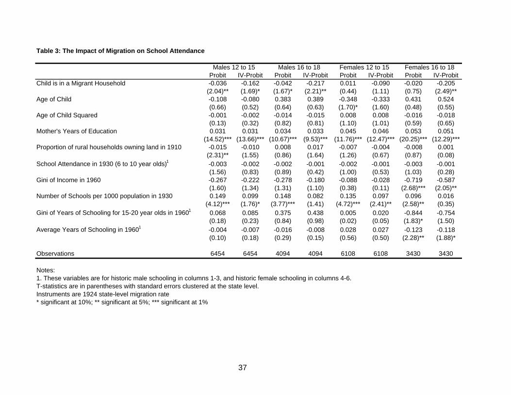
Table 3: The Impact of Migration on School Attendance

Probit IV-Probit Probit IV-Probit Probit IV-Probit Probit IV-ProbitChild is in a Migrant Household -0.036 -0.162 -0.042 -0.217 0.011 -0.090 -0.020 -0.205

(2.04)** (1.69)* (1.67)* (2.21)** (0.44) (1.11) (0.75) (2.49)**Age of Child -0.108 -0.080 0.383 0.389 -0.348 -0.333 0.431 0.524

(0.66) (0.52) (0.64) (0.63) (1.70)* (1.60) (0.48) (0.55)Age of Child Squared -0.001 -0.002 -0.014 -0.015 0.008 0.008 -0.016 -0.018

(0.13) (0.32) (0.82) (0.81) (1.10) (1.01) (0.59) (0.65)Mother's Years of Education 0.031 0.031 0.034 0.033 0.045 0.046 0.053 0.051

(14.52)*** (13.66)*** (10.67)*** (9.53)*** (11.76)*** (12.47)*** (20.25)*** (12.29)***Proportion of rural households owning land in 1910 -0.015 -0.010 0.008 0.017 -0.007 -0.004 -0.008 0.001

(2.31)** (1.55) (0.86) (1.64) (1.26) (0.67) (0.87) (0.08)School Attendance in 1930 (6 to 10 year olds)1 -0.003 -0.002 -0.002 -0.001 -0.002 -0.001 -0.003 -0.001

(1.56) (0.83) (0.89) (0.42) (1.00) (0.53) (1.03) (0.28)Gini of Income in 1960 -0.267 -0.222 -0.278 -0.180 -0.088 -0.028 -0.719 -0.587

(1.60) (1.34) (1.31) (1.10) (0.38) (0.11) (2.68)*** (2.05)**Number of Schools per 1000 population in 1930 0.149 0.099 0.148 0.082 0.135 0.097 0.096 0.016

(4.12)*** (1.76)* (3.77)*** (1.41) (4.72)*** (2.41)** (2.58)** (0.35)Gini of Years of Schooling for 15-20 year olds in 19601 0.068 0.085 0.375 0.438 0.005 0.020 -0.844 -0.754

(0.18) (0.23) (0.84) (0.98) (0.02) (0.05) (1.83)* (1.50)Average Years of Schooling in 19601 -0.004 -0.007 -0.016 -0.008 0.028 0.027 -0.123 -0.118

(0.10) (0.18) (0.29) (0.15) (0.56) (0.50) (2.28)** (1.88)*

Observations 6454 6454 4094 4094 6108 6108 3430 3430

Notes:1. These variables are for historic male schooling in columns 1-3, and historic female schooling in columns 4-6.T-statistics are in parentheses with standard errors clustered at the state level.Instruments are 1924 state-level migration rate* significant at 10%; ** significant at 5%; *** significant at 1%

Males 16 to 18Males 12 to 15 Females 16 to 18Females 12 to 15

37

Table 4: The Impact of Migration on the Education of Males Aged 12 to 15

(1) (2) (3) (4) (5) (6)Censored IV-Censored

Ordered IV-Ordered Ordered OrderedOLS 2SLS Probit Probit Probit Probit

Child is in a Migrant Household 0.151 -0.438 0.013 -0.362 -0.037 -0.512(2.13)* (1.41) (0.30) (2.24)* (0.55) (2.20)**

Age of Child 3.655 3.779 2.094 2.176 0.203 0.376(6.37)** (6.62)** (5.92)** (6.07)** (0.21) (0.39)

Age of Child Squared -0.113 -0.118 -0.061 -0.064 -0.008 -0.014(5.26)** (5.49)** (4.64)** (4.80)** (0.22) (0.40)

Mother's Years of Schooling 0.205 0.207 0.128 0.129 0.161 0.163(18.56)** (18.96)** (22.48)** (23.39)** (11.51)** (11.54)**

Proportion of rural households owning land in 1910 -0.066 -0.044 -0.039 -0.024 -0.091 -0.070(1.68) (1.15) (1.70) (1.18) (3.99)** (3.11)**

Male School Attendance in 1930 (6 to 10 year olds) 0.002 0.008 0.001 0.004 -0.005 0.000(0.42) (1.27) (0.15) (1.26) (1.09) (0.10)

Gini of Income in 1960 -1.305 -1.155 -0.766 -0.673 -1.560 -1.365(1.76) (1.43) (1.65) (1.46) (2.90)** (2.61)**

Number of Schools per 1000 population in 1930 -0.154 -0.383 -0.092 -0.239 0.240 0.026(0.96) (1.84) (0.99) (2.12)* (2.01)** (0.17)

Gini of Male Years of Schooling for 15-20 year olds in 1960 -4.336 -4.251 -2.536 -2.486 -2.625 -2.517(2.92)** (3.19)** (3.05)** (3.19)** (3.08)** (2.99)**

Average Male Years of Schooling in 1960 for 15-20 year olds -0.451 -0.471 -0.249 -0.261 -0.300 -0.313(2.90)** (2.79)** (3.00)** (3.31)** (2.73)** (2.83)**

Observations 6451 6451 6451 6451 3226 3226

Robust t-statistics in parentheses clustered at the state level.Instrument is the 1924 state-level migration rate.Censored ordered probit regressions are carried out on a 50% random sample, and use school attendance as censoring variable.* significant at 5%; ** significant at 1%

38

Table 5: The Impact of Migration on the Education of Males Aged 16 to 18



Child is in a Migrant Household 0.151 -1.366 0.041 -0.613 -0.012 -0.653(1.34) (1.99)* (0.87) (2.92)** (0.16) (2.81)**

Age of Child -3.945 -3.921 -1.716 -1.709 -1.137 -1.096(0.84) (0.82) (0.76) (0.75) (9.41)** (9.11)**

Age of Child Squared 0.120 0.119 0.053 0.053 0.033 0.032(0.87) (0.84) (0.80) (0.78) (8.15)** (7.70)**


Proportion of rural households owning land in 1910 -0.107 -0.043 -0.039 -0.011 -0.022 0.006(1.98) (0.71) (1.71) (0.55) (1.05) (0.31)

Male School Attendance in 1930 (6 to 10 year olds) -0.003 0.007 -0.002 0.002 -0.005 -0.001(0.25) (0.48) (0.40) (0.51) (1.23) (0.26)

Gini of Income in 1960 -2.173 -1.475 -0.793 -0.495 -0.167 0.142(1.56) (1.04) (1.43) (0.99) (0.35) (0.30)

Number of Schools per 1000 population in 1930 0.483 0.005 0.209 0.004 0.355 0.149(1.90) (0.01) (2.01)* (0.03) (2.91)** (1.08)

Gini of Male Years of Schooling for 15-20 year olds in 1960 -5.168 -4.690 -1.878 -1.681 -2.295 -2.117(1.76) (2.13)* (1.58) (2.02)* (2.84)** (2.64)**

Average Male Years of Schooling in 1960 for 15-20 year olds -0.574 -0.528 -0.204 -0.185 -0.218 -0.198(1.98) (1.95) (1.67) (1.97)* (0.034) (1.92)*

Observations 4094 4094 4094 4094 2047 2047


39

Table 6: The Impact of Migration on the Education of Females Aged 12 to 15



Child is in a Migrant Household 0.272 -0.225 0.125 -0.205 0.126 -0.307(3.36)** (0.77) (2.78)** (1.34) (1.53) (1.04)

Age of Child 1.613 1.671 0.748 0.787 0.475 0.477(2.18)* (2.23)* (1.81) (1.90) (0.21) (0.39)

Age of Child Squared -0.036 -0.038 -0.010 -0.012 -0.016 -0.016(1.31) (1.36) (0.66) (0.74) (0.19) (0.35)


Proportion of rural households owning land in 1910 -0.094 -0.082 -0.060 -0.052 -0.031 -0.020(3.98)** (2.82)** (3.75)** (3.37)** (1.13) (0.73)

Female School Attendance in 1930 (6 to 10 year olds) 0.002 0.007 -0.000 0.003 -0.005 -0.001(0.34) (1.00) (0.13) (0.90) (1.09) (0.11)

Gini of Income in 1960 -1.143 -0.887 -0.665 -0.496 0.323 0.561(1.61) (1.06) (1.41) (0.98) (0.50) (0.94)

Number of Schools per 1000 population in 1930 0.066 -0.112 0.086 -0.032 0.256 0.098(0.53) (0.62) (0.95) (0.29) (2.42)** (0.67)

Gini of Female Years of Schooling for 15-20 year olds in 1960 -4.061 -3.969 -2.295 -2.236 -0.798 -0.690(4.83)** (5.11)** (4.64)** (4.67)** (0.76) (0.68)

Average Female Years of Schooling in 1960 for 15-20 year olds -0.304 -0.305 -0.150 -0.150 0.088 0.087(2.94)** (2.64)** (2.57)* (2.24)* (0.61) (0.64)

Observations 6107 6107 6107 6107 3053 3053


40

Table 7: The Impact of Migration on the Education of Females Aged 16 to 18



Child is in a Migrant Household 0.338 -1.443 0.098 -0.663 0.037 -0.824(2.75)* (2.21)* (1.92) (2.83)** (0.48) (3.26)**

Age of Child 0.695 1.354 0.291 0.581 -0.236 0.128(0.19) (0.33) (0.18) (0.35) (1.62) (0.02)

Age of Child Squared -0.015 -0.034 -0.006 -0.014 0.005 -0.005(0.14) (0.28) (0.12) (0.29) (1.08) (0.02)


Proportion of rural households owning land in 1910 -0.140 -0.069 -0.052 -0.021 -0.058 -0.023(2.07)* (0.83) (1.95) (0.89) (2.27)** (0.91)

Female School Attendance in 1930 (6 to 10 year olds) -0.027 -0.006 -0.012 -0.003 -0.008 0.002(1.75) (0.39) (1.93) (0.56) (1.72) (0.41)

Gini of Income in 1960 -3.478 -2.477 -1.477 -1.054 -1.30 -0.751(1.94) (1.21) (2.10)* (1.51) (2.38)** (1.38)

Number of Schools per 1000 population in 1930 0.396 -0.270 0.184 -0.101 0.153 -0.176(1.23) (0.59) (1.45) (0.70) (1.54) (1.34)

Gini of Female Years of Schooling for 15-20 year olds in 1960 -7.445 -6.971 -2.987 -2.801 -1.846 -1.638(2.79)** (2.78)** (2.85)** (3.09)** (2.06)** (1.85)

Average Female Years of Schooling in 1960 for 15-20 year olds -0.534 -0.537 -0.218 -0.221 -0.153 -0.152(1.76) (1.56) (1.86) (1.76) (1.37) (1.33)

Observations 3431 3431 3431 3431 1716 1716


41

Table 8: Marginal Effects from Ordered Probit Models

IV-Censored IV-Censored IV-Censored IV-CensoredIV-Ordered Ordered IV-Ordered Ordered IV-Ordered Ordered IV-Ordered Ordered

Probit Probit Probit Probit Probit Probit Probit ProbitNo Schooling 0.009 0.043 0.038 0.044 0.005 0.024 0.030 0.053

(0.004)* (0.014)** (0.004) (0.012)**1 to 5 years 0.121 0.159 0.127 0.123 0.063 0.106 0.129 0.144

(0.053)* (0.041)** (0.046) (0.042)**6 years 0.001 0.137 0.078 0.080 0.006 0.117 0.103 0.115

(0.004) (0.030)** (0.006) (0.041)*7 to 8 years -0.100 0.006 -0.002 0.001 -0.052 -0.002 0.002 -0.001

(0.045)* (0.003) (0.039) (0.002)9 years -0.029 -0.225 -0.110 -0.079 -0.021 -0.145 -0.106 -0.122

(0.013)* (0.038)** (0.015) (0.036)**10 to 11 years -0.002 -0.120 -0.094 -0.039 -0.001 -0.100 -0.110 -0.046

(0.001)* (0.034)** (0.001) (0.042)**12 years or more n.a. n.a. -0.036 -0.130 n.a. n.a. -0.047 -0.145

(0.013)** (0.017)**n.a. denotes not applicable, as 12 to 15 year olds have not reached 12 years of schooling.* significant at 5%; ** significant at 1%

Males 12 to 15 Males 16 to 18 Females 12 to 15 Females 16 to 18

42

Table 9: Interaction of Migration with Mother's Schooling

Males Males Males Males Females Females Females Females12 to 15 12 to 15 16 to 18 16 to 18 12 to 15 12 to 15 16 to 18 16 to 18

(1) (2) (3) (4) (5) (6) (7) (8)2SLS 2SLS 2SLS 2SLS 2SLS 2SLS 2SLS 2SLS

Child is in a Migrant Household -0.201 -0.538 -1.244 -1.741 0.138 -0.520 -0.817 -2.211(0.52) (1.48) (1.51) (2.16)* (0.31) (1.44) (0.94) (2.53)*

in a Migrant Household *Mother's Years Schooling -0.072 -0.042 -0.098 -0.187(1.43) (0.34) (1.34) (1.34)

in a Migrant Household * Low Mother's education 0.355 0.796 0.489 1.090(1.03) (1.43) (1.60) (1.82)

Observations 6451 6451 4093 4093 6107 6107 3431 3431Robust z statistics in parentheses* significant at 5%; ** significant at 1%Regressions also include all controls in Tables 3-6.

43

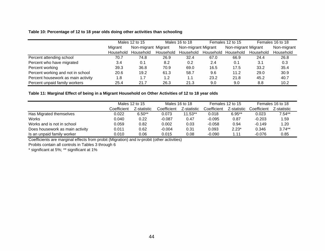
Table 10: Percentage of 12 to 18 year olds doing other activities than schooling

Migrant Non-migrant Migrant Non-migrant Migrant Non-migrant Migrant Non-migrantHousehold Household Household Household Household Household Household Household

Percent attending school 70.7 74.8 26.9 32.4 67.0 66.9 24.4 26.8Percent who have migrated 3.4 0.1 8.2 0.2 2.4 0.1 3.1 0.3Percent working 39.3 36.8 70.9 69.0 16.5 17.5 33.2 35.4Percent working and not in school 20.6 19.2 61.3 58.7 9.6 11.2 29.0 30.9Percent housework as main activity 1.8 1.7 1.2 1.1 23.2 21.8 45.2 40.7Percent unpaid family workers 25.4 21.7 26.3 21.3 9.0 9.0 8.8 10.2

Table 11: Marginal Effect of being in a Migrant Household on Other Activities of 12 to 18 year olds

Coefficient Z-statistic Coefficient Z-statistic Coefficient Z-statistic Coefficient Z-statisticHas Migrated themselves 0.022 6.50** 0.073 11.53** 0.018 6.95** 0.023 7.54**Works 0.040 0.22 -0.087 0.47 -0.095 0.87 -0.203 1.59Works and is not in school 0.059 0.82 0.002 0.03 -0.058 0.94 -0.149 1.20Does housework as main activity 0.011 0.62 -0.004 0.31 0.093 2.23* 0.346 3.74**Is an unpaid family worker 0.010 0.06 0.015 0.08 -0.090 1.11 -0.076 0.85Coefficients are marginal effects from probit (Migration) and iv-probit (other activities)Probits contain all controls in Tables 3 through 6* significant at 5%; ** significant at 1%



44

can migration reduce educational attainment? evidence from...

Documents