Munich Personal RePEc Archive

Can portfolio diversification increase

systemic risk? evidence from the U.S

and European mutual funds market

Dicembrino, Claudio and Scandizzo, Pasquale Lucio

University of Rome ’Tor Vergata’

30 November 2011

Online at https://mpra.ub.uni-muenchen.de/33715/

MPRA Paper No. 33715, posted 30 Nov 2011 19:04 UTC

1

Can Portfolio Diversification increase Systemic Risk?

Evidence from the U.S and European Mutual Funds Market1

Pasquale Lucio Scandizzo

CEIS, University of Rome “Tor Vergata”

Claudio Dicembrino

CEIS, University of Rome “Tor Vergata” and ENEL SpA

Abstract

JEL classification: G01, G11, G32

1 The views expressed in this article are solely those of the authors and do not involve the institutions of affiliation. All

other usual disclaimers apply. Corresponding author: Claudio Dicembrino (dicembrino@economia.uniroma2.it).

This paper tests the hypothesis that portfolio diversification can increase the threat of systemic

financial risk. The paper provides first a theoretical rationale for the possibility that systemic

risk may be increased by the proliferation of financial instruments that lead operators to hold

increasingly similar portfolios. Secondly, the paper tests the hypothesis that diversification may

result in increasing systematic risk, by analyzing the portfolio dynamics of some of the major

world open funds.

2

Keywords: Systemic Risk, Portfolio Diversification, Mutual Funds, CAPM

Introduction

This paper contributes to the growing literature on the link between portfolio diversification

and its implications on the question of systemic risk. We first show that the introduction of any

contingent claim, whose value is correlated with the value of the assets owned by a population of

heterogeneous agents, causes an improvement of the agents‟ expected utility. At the same time,

such an introduction will increase overall systemic risk. These effects are due to the cumulative

interaction of two distinct, but closely related factors:

(i) The gain obtained from diversifying one‟s portfolio, thus reducing risk exposure

through risk sharing;

(ii) The gain obtained through risk shifting from higher to lower risk-aversion agents.

We test the hypothesis on the negative relationship between diversification and systemic risk

by estimating a simultaneous equation model on a panel of the 266 largest mutual funds (based on

size). In particular, we use 162 funds to analyze the US market and 64 funds for the European area,

exchanged in the market between January 2003 and March 2010. The plan of the paper is as

follows. In section 1, we review the basic concepts and some of the recent literature on systemic

risk. In section 2, we look in particular at the relationship between diversification and systemic risk.

In Section 3, we develop a theoretical model that captures the essence of this relationship, by

analyzing the effects on both diversification and systemic risks of the issuance of an additional

security. In section 4 we describe the data set. In Section 5 we present the econometric analysis and

the results obtained. In the last section we discuss some conclusive remarks.

1. On the Meaning and the Measure of Systemic Risk

In the context of analysis of financial instability, an active debate has emerged around how to

define both a systemic event, a systemic risk, and their effects. Despite the considerable amount of

literature on the topic, no shared consensus exists about the meaning, features and policy

implications of these concepts. Highlighting the complexity of these issues, Alan Greenspan (1995),

as chair of the Federal Reserve System (FED), has underlined that “the very definition of systemic

risk is somewhat unsettled”.

Macro-level analyses of systemic risk can be found in several works of the past two decades.

Kaufman et al. (2003) refer to systemic risk as the risk or the probability of collapse in an entire

financial system. Bartholomew et al. (1995) examine, within the systemic risk spreading

3

mechanism, its effect not only on the domestic economy, but also on the entire international

banking, financial, or economic system. Mishkin (1995) focuses on the investment repercussions of

such an important event. Allen and Gale (2000) analyze the cause-effect process through which

macro-shocks can spark contagion episodes and bank runs. Bordo et al. (1998) define systemic risk

as a situation where “shocks to one part of the financial system lead to shocks elsewhere, in turn

impinging on the stability of the real economy” (pp. 31). In their exhaustive review of the literature,

De Bandt and Hartmann (2002) offer a similar view of a systemic event, saying that it takes place

when a shock affects “a considerable number of financial institutions or markets in a strong sense”

(p.11). De Nicolò and Kwast (2002), and Dow (2000), define systemic risk as a mechanism that, at

the same time of the shock, affects the entire financial system, while Lehar (2005) says that “a

systemic crisis can be defined as an event in which a considerable number of financial institutions

default simultaneously”.

The search of the micro foundations of systemic risk across shock-transmissions and

spillover effects on the entire financial system has given rise to a different strand of literature. The

following contributions emphasize causation mechanisms requiring close and direct connections

among several institutions and different markets. Kaufman (1995) underlines the fact that systemic

risk is the probability that cumulative losses originate from an event that, through a contagion

effect, involves a chain of institutions belonging to a market. The Board of Governors of the FED

(2001) provides a definition whereby systemic risk jeopardizes the solvency capacity of

institutions2. Kambhu et al. (2007) define systemic risk as a situation where financial shocks “have

the potential to lead to substantial, adverse effects on the real economy, e.g., a reduction in

productive investment due to the reduction in credit provision or a destabilization of economic

activity”. This contribution has stressed the transmission of financial events to the real economy, as

the key feature distinguishing a systemic event from a purely financial event. The contagion effect

indiscriminately affects more or less the entire universe reflecting a general loss of confidence in all

the units (solvent and insolvent) involved in the system. Referring not only to bankruptcy but also

to the default of all market participants, the G-10 “Report on Financial Consolidation” (2001)

defines systemic risk as: “…a risk that an event will trigger a loss of confidence in a substantial

portion of the financial system that is serious enough to have adverse consequences for the real

economy”. In Bartram et al. (2005), systemic risk affects the unexposed institutions not otherwise

involved by a crisis given its economic fundamentals.

2 “Private large-dollar payments network were unable or unwilling to settle its net debt position. (…) Serious

repercussions could, as a result, spread to other participants in the private network, to other depository institutions not

participating in the network, and to the nonfinancial economy generally”.

4

Overall, we can conclude that despite the vast literature on systemic risk, a clear and shared

view of the concepts underlying this term has not emerged. Nevertheless, in the attempt to provide

a general and unambiguous definition of systemic risk, both at a macro and micro level, three

principal aspects must be recognized:

1. Impact on a “substantial portion” of the financial system;

2. Spillovers from one institution to many others;

3. Strong and adverse macroeconomic effects.

Turning again to the literature, we have carried out a review of systemic risk measures,

according to two broad categories of indicators:

a) Traditional macroeconomic indicators of financial soundness and stability;

b) Indicators of interdependencies among financial institutions through the analysis of the

financial institution‟s assets.

The first group of measures relies on bank capital ratios and bank liabilities to show that

aggregate macroeconomic indicators can provide a valid and useful instrument to predict systemic

financial threats. Through the study of macroeconomic fundamentals, Gonzalez-Hermosillo et al.

(1997), Gorton (1998) and Gonzalez-Hermosillo (1999) demonstrate how macro analysis can be

appropriately used to estimate systemic risk. More recently, Bhansali et al. (2008) derive a

“systemic credit risk” variable from aggregate index credit derivatives, finding that this measure of

systemic risk roughly doubles during the 2007-2009 financial crisis as compared to May 2005. De

Nicolò and Lucchetta (2009) use a dynamic factor model to work out joint forecasts of indicators of

systemic real risk and systemic financial risk, and then elaborate stress-tests of these indicators as

impulse responses to structurally identifiable shocks.

The second group of measures quantifies the linkages among financial institutions as well

as exposures among banks that through their business can influence each other in situations of

financial distress. A more recent contribution is given by Lehar (2005), assessing the probability

that a certain number of banks within a specific arc of time go bankrupt due to reduced asset value

vis a vis a critical and well-defined liability value. Adrian and Brunnermeier (2009) define CoVaR

as the VaR of financial institutions conditional on other institutions that experience, at the same

time, financial distress. De Nicolò and Lucchetta (2009) investigate the transmission channels and

contagion effects of certain shocks between the macroeconomy, the financial markets and the

intermediaries. Huang et al. (2010) use as a proxy of systemic risk, the price of insuring a dozen of

5

the major U.S banks against financial turmoil on the basis of both ex-ante bank default probabilities

and forecasted asset-returns correlations.

The IMF (2009) surveys four different methods to assess interlinkages among financial

institutions:

The network approach, where the interbank market spreads the transmission of financial

stress through the banking system (Allen et al. (2010));

The co-risk model, (or co-movement risk model) whereby the probability default of one

institution is directly linked to the default risk of another institution (Adrian et al. (2009,

p.5)), de Vries et al. (2001), Longin and Solnik (2001) and Chan-Lau (2004);

The distress dependence matrix based on the probability of default of banks‟ pairs, taking

into account a panel of financial institutions Goodhart and Segoviano (2009);

The default intensity model based on the estimate of the probability of default of financial

institutions Giesecke and Bacho (2009)).

Among other contributions that are worth mentioning, Bartram et al. (2005) propose three

different approaches to estimate systemic risk by observing market reaction to global financial

shocks for a subset of banks that are not directly exposed to the shock3. Capuano (2008) develops a

framework to derive a market-based measure of probability of default, defined as the probability

that the value of the underlying asset will fall below a given threshold. Using a VaR approach,

Acharya et al. (2010), define systemic risk as the likelihood of experiencing cumulative losses in

financial system that exceed the predicted by VaR model.

2. Systemic Risk and Portfolio Diversification

Recalling the 2008 financial crises, characterized by a conglomerate of interrelated financial

services and multi-sector institutions, a vibrant discussion has emerged regarding the causes of the

recent financial system collapse. In this debate, many financial actors have been analyzing the roots

of this phenomenon: on one side, many address as micro-drivers of this turmoil the financialization

of the real economy (e.g. mortgage-backed securities (MBS)); others, on the other side, highlight as

macro-drivers the lack of an efficient macro-prudential banking system (e.g. timely mechanisms

able to prevent contagion and spread). In this current framework, Rodrìgez-Moreno et al. (2010)

3 Bertrand et al. (2005) argue that in efficient capital markets, negative information (as 9/11) will affect bank

performances that are exposed to the events in question. Unexposed banks will be unaffected by these effects.

6

argue that academic research has widely investigated both idiosyncratic and systematic risk,

ignoring the fundamental importance of systemic risk and its implications on the financial markets.

This concept is also clearly expressed in Masera et al. (2010), stating “it is now clear that

supervisory authorities, policy makers and political authorities must look, beyond idiosyncratic

risk, also at the systemic risk to the broader financial system that certain very large financial firms

(Systemically Important Financial Institutions – SIFIs) pose”.

Further, what appears to have been less investigated in the relevant literature are the potential

effects of portfolio diversification on systemic risk. While the benefits of diversification at a

microeconomic level (in portfolio choices theory) have been thoroughly examined in the economic

literature (Allan and Gale, 2005; Freixas et al., 2005; and Wagner and Marsh, 2006), the

macroeconomic side of the link between diversification and systemic risk remains complex, multi-

faceted, and not yet completely explored (Lo, 2008). In this regard, two different views, outlining

both the negative and positive effects of the relationship between diversification and systemic risk,

have been characterizing this more controversial strand of the literature. Although portfolio

diversification reduces risks at each individual institution, from the prospective of the entire

financial system, it only reallocates these individual risks (Wagner, 2009). As argued in de Vries

(2005) “…while diversification reduces the frequency of individual bank failures, since smaller

shocks can be easily borne by the system, at the same time diversification makes the bank sector

prone to systemic breakdowns in case of very large (non-macro) shocks, which otherwise would

only have isolated impact”. Indeed, there is not any evidence to date, which would indicate that

portfolio diversification reduces the threat of systemic risk. Further diversification leads to sharing

risks across institutions involved in contributing to make these positions similar to each other, with

the effect of facilitating financial contagion due to interlinked relationships among financial

institutions. Nevertheless, it is crucial to include in these causes even the large financial

conglomerates and the increasing presence of derivative instruments in the international financial

system. In particular, derivative products have been indicated as both a responsible mechanism and

perverse interaction of risk spreading and transferring from the banking to the insurance sector and

vice versa (e.g. Originate-to-Distribute Model in banking and OTC derivatives).

In this regard, risk transfers between insurers and the banking sector represent a widely used

diversification instrument, allowing banks to transform liquid liabilities of depositors into illiquid

assets (loans) (de Vries 2010). Furthermore, and in particular during the last decade, there are many

contributions sustaining the contention that diversification has negative effects on the financial

system, including De Young and Roland (2001), Stiroh (2004, 2006), Acharya et al. (2006), and

Hirtle et al. (2007). In particular, Stiroh and Rumble (2006) find that benefits stemming from

7

diversification can be completely undermined by the volatility effect of new exposures introduced

into a portfolio. Sanya et al. (2010) offers different kinds of mechanisms that can be detected to

analyze the negative impact (or reduced benefits) of portfolio diversification on systemic risk. The

first, discussed in Froot and Stein (1998) and Cebenyoyan and Strahan (2004), indicates that gains

obtained from portfolio diversification will be limited if the banks (managing the portfolio) do not

have a risk efficient portfolio. The second argues that diversification can play a negative role when

banks expand their business into industries, with difficulties emerging from loan-monitoring

activities. Wegner (2006) emphasizes the role of diversification as an incentive for taking greater

and new risks in the international financial markets. De Vries (2010) states that “diversification

lowers the risk of isolated shocks for a financial entity, but may simultaneously increase the

systemic risk”. Recently, Allen et al. (2010) claim that the spread of credit default swaps and other

credit derivative products, loan sales and collateralized loan obligations, has increased and

improved the possibility for banks, mutual funds and financial institutions to diversify risk. But this

possibility has, according to Allen et al. (2010) “also led to more overlap and more similarities

among their portfolios. This has increased the probability that the failure of one institution is likely

to coincide with the failure of other similar institutions” (p.6).

Conversely, there is an opposing strand of the relevant economic literature which sustains the

positive effects of diversification, first, from an efficiency gain point of view (Berger et al. (1999),

Estrella (2002)), and second, in increasing bank stability (Grossman (1994), Wheelock (1995),

Berger et al. (1999), Reichart and Wall (2000), Campa and Kedia (2002), and Baele et al. (2007)).

3. The model

Consider an economy formed by n agents. Each agent is endowed with a certain amount of

wealth, whose rate of return varies stochastically from one agent to the other. The satisfaction of the

i-th agent is measured by expected utility )( ii yEU , where E is the expectation operator, (.)iU

denotes a well behaved utility function and iy is stochastic income. By projecting orthogonally the

agent‟s stochastic individual income iy onto the stochastic total agents‟ income i

iyy , we can

write the following identity:

(1) iiii vyy )(

where 0i

i

v 0iEv , ,0),( yvCov i iiEy ;

i

in

1; and ni

i

.

8

Equation (1) decomposes individual risk into a systemic, diversifiable component, correlated

with total agents‟ revenue, and into an independent, idiosyncratic component.

The variance of individual income, assuming no correlation between diversifiable and

idiosyncratic risk is:

(1bis) 222)( iyiiyVar

By diversifying, each operator can bring her i

to unity, thus bringing her portfolio to

coincide with the market portfolio, which by definition is the most diversified, being an average of

all portfolios, thereby achieving a minimum variance (i.e. the variance of the most diversified

portfolio).

The distribution function (d.f.) of total revenue is )(yF and its support is the compact

interval ],0[ maxy , while the d.f. of the idiosyncratic component is )( ivG over the support

],[ maxmin ii vv .

Assume now that a derivative is introduced. In our context a derivative is defined as a

contingent claim whose value depends on one of the assets, i.e. income sources in the market, more

specifically, we will assume it depends on the average return of all other assets. The derivative

price )( yp is assumed to be distributed with mean Ep , variance 2

p and covariance ip with each

agent‟s income. The derivative corresponds to a contract between a issuer (i.e. a short holder) and

a buyer ( a long holder), whereby each party promises to pay the other a premium in different states

of the world.

The i-th agent is confronted with the problem of choosing an optimal number of units of the

derivative to hold long (i.e. to purchase) or short (i.e. to issue), so that total income for each agent

will be equal in each state of nature to the solution of the following maximization problem:

(2) )( iiq

xxEUaMi

, pqyx iii ; ni ...2,1

where iq denotes the number of units of the security in terms of shares of the promised (random)

payoff p , and is positive or negative according to whether the security is bought or sold by the ith

agent.

Using (1) and the related assumptions, the expected utility in (2) can be written as follows:

9

(3) max

min

max

0

)()())()(()(i

i

v

v

y

iiiiiiii vdGydFypqvyUxEU

)())()((max

0

ydFypqymV i

y

iii

where iiim and (.)iV is the indirect utility function defined as:

(4) max

min

)()()(i

i

v

v

iiiii vdGvmUmV for all i

As shown by Kihlstrom, Romer and Williams (1981), the indirect utility function in (4) is well

behaved, i.e. it is increasing and concave in its arguments.

In order to show that the introduction of the security increases the income of the i-th subject,

it is sufficient to show that the problem in (2) has a solution with a non zero value for the security in

question. The first order condition is obtained differentiating (3) w.r.t. iq :

(6) 0)()())(( '

0

'max

pVEydFypVdq

dEVi

y

i

i

i ,

where primes indicate derivatives, while the second order condition requires:

(7) 0)( 2''

2

2

pVEdq

EVdi

i

i ,

which is always satisfied for a concave utility function. Applying the definition of covariance to (6),

we obtain:

(8) 0))(( '' ypVCovEyEV ii

Differentiating totally with respect to the parameters yields:

(9) 0)]()([)]()([ ''''2'''''

iiiiiii dpyVCovEppyVEdqpVCovEppVEdEpEV

which, by applying again the definition of covariance, can be also be written as:

(10) 0)()( 2''2'''

iiiii dypVEdqpVEdEpEV

10

Since 0)(

'

2''

i

ii

EV

pVE and 0

)('

2''

i

ii

EV

ypVE are both positive measures of risk

aversion, solving (10) for idq yields:

(11) i

i

i

i

i ddEp

dq

Equation (11) establishes the fact that any increase in the expected pay off and/or in

the beta will increase long positions while it will reduce short positions in the derivative asset. In a

stable market equilibrium, we must have n

i

idq1

0 , which implies:

(12) ddEp

where m

i i

n1

1)1

( and n

i

i

i

i

nd

1

1.

Substituting (12) into (11) yields the equilibrium relationship:

(13) dddqi

i

i

i

i

Expression (13) establishes the dependence of the quantities traded of the security on the

difference between the individual incentive to diversify (through his beta and risk aversion) and the

incentive to shift risk to or from more risk averse traders.

Expression (13) can be integrated, assuming that the utility function parameters are constant.

A simpler way to proceed, however, is to expand '

iV in (8) according to the Mac Laurin‟s formula:

(14)

2

0

'''

0

''

0

'

0

' ))((2

1))(( ypqymVypqymVVV iiiiiiiiii

where the subscripts 0 and denote the fact that the derivatives of the utility function are

measured, respectively, at the origin and at )( pqy ii, with 10 .

11

Substituting into (8), and assuming that all moments higher than two of the joint distribution

of y and p are zero, yields:

(15) 0)( 2

piypii qEp

where '

''

0

i

i

iEV

Vis a measure of absolute risk aversion and coincides with the Pratt coefficient for

the family of constant risk aversion utility functions (CARA).

Solving (15) for iq , we obtain:

(16) 22

p

yp

i

pi

i

Epq

Expression (16) shows that a solution to the maximization problem is the result of two factors

of agents‟ heterogeneity: (i) the degree of risk aversion and, (ii) the correlation between the security

payoff and the agent income. However, in order for the solutions for the different agents to be

mutually compatible, the determination of the expected payoff Ep should be competitively

determined, i.e. i

iq 0 , so that :

(17) ypEp

where i i

n1)

1( is the harmonic average of the individual risk aversion coefficients and I

have used the property : n

i

i n1

.

Substituting (17) into (16) yields:

(18) )()(i

iii

i

iq

where 2

p

yp and

)2()])([))(( 22

jpp

ji

iin

i

i ypqVar

In conclusion, each agent will be able to improve her expected utility by diversifying into a

short or long position on an additional contingent claim, depending on two effects: (i) the difference

between average and individual demand for diversification (the beta) and, (ii) the difference

12

between average and individual risk aversion. The equilibrium level of long and short positions will

be independent from the expected level of the pay off, but will depend only on its variance. For

example, in the special case of a derivative that acts as an insurance (e.g. a put option) and pays to

long holders yRp when Ry and cp otherwise, we have that )(22 RFyp and

)(2RFyyp , so that 1 and :

(19) )(i

iiq

and

)()()()20( ypvyxi

iiiiii

so that : )2()()( 222222

j

jpp

i

iiiyiixVar .

Note that the introduction of the security has improved expected income of each agent, it has

further diversified her portfolio, but, at the same time, has introduced a new source of variance

(and, implicitly, risk), into the system. This new form of risk can be defined as “systemic”, because

it depends on the correlation between the yield of the derivative and the income of all agents in the

system. In other words, a shock on the price of the derivative is transmitted to all agents.

From equation (20), we can derive a modified version of the well known CAPM model, by

subtracting from both sides the risk free rate of return r:

)()()()()21( ypvryrxi

iiifiiifi

4. Dataset

As noted in section 2, several methodologies have been implemented to measure systemic

risk, based on different motivations and goals: we choose the correlation among mutual funds

showing lower performances compared to the average level returns (threshold value) as a proxy of

systemic risk (Syst_rsk). The choice of this approach is not novel in the literature (De Nicolo and

Kwast (2002)), its advantage being that correlations among funds‟ returns are considered as a

forward-looking variable much more suitable than balance sheets or company financial indicators to

capture systemic failures and the associated costs. Furthermore, the correlation between returns of

different funds reflect fund values. Following the approach by Chan et al. (2004), we thus estimate

13

this variable through a pairwise correlation approach between the return of the i-th and the j-th

fund:

(23)

Cov Ri,tR j,t

i j

2

i

2 2

,i

2

j

2 2

,i

2

As discussed above, we propose the systemic risk variable as the pairwise correlation within

the subset of funds having lower than average performance:

Rij,t x ij,t x ij

_

if x it,t x ij

_

Rij,t 0 otherwise

We analyze a panel of the 226 largest mutual funds (based on size) from the Morningstar

database4. The U.S. market is analyzed through 162 funds and through 64 funds for the European

area, exchanged in the market between January 2003 and March 2010, thereby amounting to 19.662

monthly observations. We chose as the risk-free rate for the U.S market the 3-Months Treasury

Bills from the Federal Reserve Bank of Saint Louis (FED of Saint Louis) database. For the

European market, we use the 3-Months German government bond from the Bloomberg database.

Through a Return Based Style Analysis (RBSA), we create a return weighted index able to capture

the equity stocks, government bonds and corporate fund performances. Bond, equity and cash

compose the n-segments of any fund in the n-th portfolio.

In order to build up these two proxies (for both the U.S and European market) we consider:

the U.S and European Morgan Stanley (MSCI) index for government bonds;

the U.S and European J.P Morgan (JPM EMBI) index for the stock exchange;

the U.S and European Merry Lynch (ML-Corporate) index for the corporate sector.

4 The largest funds are chosen by size. Having our database comprised of 226 mutual funds exchanged in n different

countries, we divide these mutual funds into three wide macro-areas of affiliation. Europe = Austria, Belgium, Finland,

France, Germany, Ireland, Italy, Luxembourg, Netherlands, Portugal, Spain, Sweden, Switzerland and the United

Kingdom. North America = United States, Canada and Mexico.

14

Figure 1: US market performances

Source: Authors‟ elaborations on Bloomberg database. The “weighted” index is the market index created on the

other three index performances.

Figure 2: EU market performances

Source: Authors‟ elaborations on Bloomberg database. The “weighted” index is the market index created on the

other three index performances.

The Libor-OIS (Overnight Interest Swap) (Libor_Ois) for the American market, and the

spread Euribor-Ois (Euribor_Ois) for the European market are considered as proxies for banks‟

soundness and as a reliable indicator of the stability of the banking system5. The diversification

5 The importance of this spread is asserted both by Alan Greenspan “Libor-OIS remains a barometer of fears of bank

insolvency” and the Vice President of the FED of St. Louis, D.L. Thornton “the term Libor-OIS spread is assumed to be

15

index (DIV) has been measured as the difference from each portfolio , in terms of asset allocation,

and an equally diversified portfolio. The variable Beta Market (ßmkt) is the difference between the

return weighted index previously mentioned and the risk free rate (see above); while the Excess

Return (Exc_Ret) is the difference between the mutual fund returns and the risk free rate (see

above) , for both the U.S and European markets. The Consumer price index growth rate (Cpi) for

the U.S and the Harmonised Index of Consumer Prices (HICP)6 for Europe represent the two

variables accounting for inflation. The 2007, 2008 and 2009 (D07, D08, D09) dummy variables

take into account the years where the last crisis created increased turbulence in the financial

markets. A detailed list of the variables used in the empirical analysis is presented in Table 1.

5. The Estimation Strategy and the Empirical Results

We estimate a simultaneous equation model, based on the classical CAPM formulation

augmented by a variable that represents the contribution that diversification through derivatives

makes to systemic risk. In Tables 2 and 3, we show the result of the CAPM estimates in the two

markets (U.S and Europe). In particular, using the CAPM specification presented in Fama et al.

(2004), we regress individual (fund) excess returns on market returns, the diversification index

and a series of dummy variables. In both markets, we find a positive relation between Beta and

excess returns. Although the two markets show a significant difference in their Beta coefficients,

(approximately 1.16 in the U.S and around 0.86 in the European market) no sizeable variation

appears in intra-market differences (the U.S market beta ranges between 1.14 and 1.17 while the

European market beta varies between 0.84 and almost 0.89). In the U.S and European market, the

diversification variable shows a positive and a high significant coefficient, while the systemic risk

variable negatively impacts the excess returns (dependent variable).

Once we examined the CAPM analysis, in order to assess the impact of the diversification

strategy on systemic risk, we specify a model in which the market excess returns and the indicators

of systemic risk are simultaneously determined and depend on a series of key variables that,

according to the literature, play a fundamental role both in influencing the beta market and as a

possible factor impacting systemic risk. The model is estimated by using two stage least squares.

The first equation is given by:

a measure of the health of banks because it reflects what banks believe is the risk of default associated with lending to

other banks”. 6 Consumer price inflation in the Euro area is measured by the Harmonised Index of Consumer Prices (HICP). The

HICP is compiled by Eurostat and the national statistical institutes in accordance with harmonised statistical methods

(http://www.ecb.int/stats/prices/hicp/html/index.en.html).

16

(22a) - U.S. Market:

Mkt_Betai,t Sist_ rski,t Fcorri,t Cpii,t Libor_Oisi,t D08i D09i ut

(22b) - European Market:

Mkt_Betai,t Sist_ rski,t Fcorri,t HICPi,t Euribor_Oisi,t D08i D09i ut

Equations (22a-b) test the hypothesis that systemic risk variable has a negative impact on

the market performances. In addition to the dependent variable Mkt_Beta, measured as the market

monthly excess return, the independent variables are: the systemic index measured as the fund

correlations (without any return threshold); the consumer price index growth rate (for the American

market) and the Harmonised Index of Consumer Prices (for the European market); the spread

Libor-Ois (Libor_Ois) for the American market; the spread Euribor-Ois (Euribor_Ois) for the

European market as proxies of bank sector soundness; and the 2007, 2008 and 2009 dummy

variables on the Market Beta variable (Mkt_Beta), (defined as difference between market

performance, created through the RBSA, and the risk free rate).

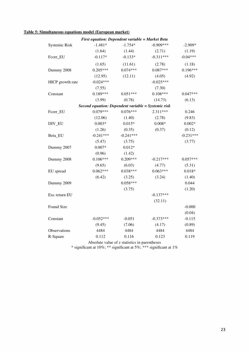
As tables 4-5 show, an increase in the correlation of mutual funds‟ returns (Fcorr) has a

negative and significant impact on market excess returns (Mkt_Beta). This effect is strongly

significant in both the U.S and EU markets. These findings clearly emerge from the tests applied

through the first hypothesis in any specification of the 22a-b models. The Libor (Euribor)-OIS

spread represents the unsecured interest rate at which banks lend money to other banks which must

satisfy certain criteria for creditworthiness. Libor and Euribor are not entirely credit risk-free,

because they reflect both liquidity risk and the bank‟s default risk over the following months. The

OIS represents the average of the overnight interest rates expected until maturity, so the Libor

(Euribor) – OIS reflects both the liquidity and default risks over the next months. Then, during the

period where the stock markets register a strong performance, this spread should be subjected to a

reduction. In this context, our results confirm the negative relationship between market performance

and the Libor (Euribor) – OIS spread indicator. The Cpi and Hicp negative coefficients support the

strand of the literature that predicts a negative relationship between inflation and stock

performances in the short run.

In the second equation of the simultaneous model, (23a-b) we aim to test the second

hypothesis, i.e. that an increase in the similarities of the diversification strategies of each fund can

increase the threat of systemic risk. In this case the dependent variable is the systemic risk, while the

independent variables are the three dummy variables for 2007-2008-2009, the fundsize and the

Cpi/Hicp growth rate on the systemic risk variable.

17

(23a) - U.S. Market:

Sist_ rski,t Mkt_Betai,t Fcorri,t Cpii,t Libor_Oisi,t Divi,t Fsizei,t D07i D08i D09i ut

(23b) - European Market:

Sist_ rski,t Mkt_Betai,t Fcorri,t HICPi,t Euribor_Oisi,t Divi,t Fsizei,t D07i D08i D09i ut

The results of the empirical analysis are contained in table 4 for the U.S market, and table 5

for the European market. In general all these variables show a high level of significance, although

the diversification index variable is weakly significant at 10%. The strategy in the asset allocation

investment choices is captured by the diversification index (Div) variable. This index explains how

portfolio diversification can increase the threat of systemic risk as dependent variable. The

similarities in fund returns for each portfolio are instead represented by the Fcorr that also shows a

positive and significant coefficient. This suggests that an increase of the correlation among fund

returns can be interpreted as a warning for a distress situation in the financial system. As already

explained in the first stage, in periods when the stock markets register good performances, this

measure is subjected to a reduction, conversely in periods of turmoil this spread should increase so

as to capture the market risks. In the estimate of the second equation, we thus find that an incrase of

this spread leads to an increase of the threat of systemic risk. Further in both specifications (model

23a-b) we find a positive relation between the dummy variables, the Fund size and the CPI (for the

American market) or the Hicp (for the European market) and the systemic risk variable. The Market

Beta variable has a negative effect on systemic risk, suggesting that deteriorating market

performance reverberates negatively on systemic risk.

6. Concluding Remarks

The theoretical and empirical motivation of this analysis is the ongoing debate which

posits that derivative driven financial diversification, often interpreted by professionals and

academics as a fundamental benefit of investment financial strategies, can be undesirable and a

driver of excessive instability. Our results provide insight into the connection between portfolio

diversification strategies and the impact on systemic risk. In this regard, we have developed a model

where the i-th agent diversification strategy interacts with the j-th agent diversification strategy,

through the mutual purchase and sale of derivatives, thus increasing agents‟ interdependence, the

probability of contagion from a systemic event and, ultimately, systemic risk. The basic reason for

18

this result is that derivatives provide an insidious instrument of diversification. While they appeal to

risk managers because of their capacity, as contingent claims, to provide insurance to individual

investors, at the same time, they create a separate source of portfolio volatility which may be

increasingly difficult to further diversify.

Some of the implications of the theoretical model have been tested through a simultaneous

equations model, where we have hypothesized that systemic risk may increase the need to further

diversify and, at the same time, further diversification, by increasing portfolio similarities, can boost

systemic risk. Both hypothesis appear to be corroborated by our econometric tests, which show

significant and mutual substantial impacts of the signs implied by the model, between

diversification and systemic risk variables.

Our findings can be summarized as follows: from the point of view of the individual agent,

the portfolio diversification strategy represents a valuable instrument of portfolio management.

However, from the point of view of the financial system, when such a diversification is pursued

through a proliferation of derivative securities, the increase in similarities and mutual

interdependence among financial agents may result in an increase in aggregate risk. Such an

increase has systemic nature since it is based on the loss of a diversified ensemble of financial

agents as a key source of systemic resilience.

19

List of tables

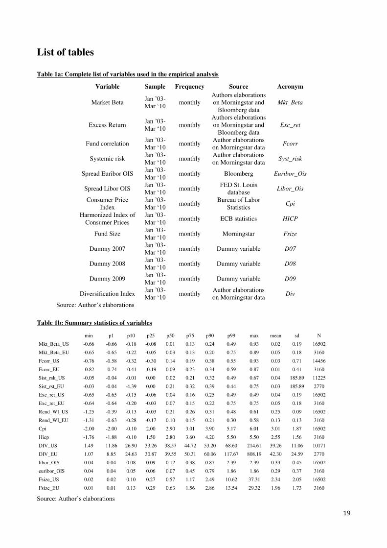
Table 1a: Complete list of variables used in the empirical analysis

Variable Sample Frequency Source Acronym

Market Beta Jan ‟03-

Mar „10 monthly

Authors elaborations

on Morningstar and

Bloomberg data

Mkt_Beta

Excess Return Jan ‟03-

Mar „10 monthly

Authors elaborations

on Morningstar and

Bloomberg data

Exc_ret

Fund correlation Jan ‟03-

Mar „10 monthly

Author elaborations

on Morningstar data Fcorr

Systemic risk Jan ‟03-

Mar „10 monthly

Author elaborations

on Morningstar data Syst_risk

Spread Euribor OIS Jan ‟03-

Mar „10 monthly Bloomberg Euribor_Ois

Spread Libor OIS Jan ‟03-

Mar „10 monthly

FED St. Louis

database Libor_Ois

Consumer Price

Index

Jan ‟03-

Mar „10 monthly

Bureau of Labor

Statistics Cpi

Harmonized Index of

Consumer Prices

Jan ‟03-

Mar „10 monthly ECB statistics HICP

Fund Size Jan ‟03-

Mar „10 monthly Morningstar Fsize

Dummy 2007 Jan ‟03-

Mar „10 monthly Dummy variable D07

Dummy 2008 Jan ‟03-

Mar „10 monthly Dummy variable D08

Dummy 2009 Jan ‟03-

Mar „10 monthly Dummy variable D09

Diversification Index Jan ‟03-

Mar „10 monthly

Author elaborations

on Morningstar data Div

Source: Author‟s elaborations

Table 1b: Summary statistics of variables

min p1 p10 p25 p50 p75 p90 p99 max mean sd N

Mkt_Beta_US -0.66 -0.66 -0.18 -0.08 0.01 0.13 0.24 0.49 0.93 0.02 0.19 16502

Mkt_Beta_EU -0.65 -0.65 -0.22 -0.05 0.03 0.13 0.20 0.75 0.89 0.05 0.18 3160

Fcorr_US -0.76 -0.58 -0.32 -0.30 0.14 0.19 0.38 0.55 0.93 0.03 0.71 14456

Fcorr_EU -0.82 -0.74 -0.41 -0.19 0.09 0.23 0.34 0.59 0.87 0.01 0.41 3160

Sist_rsk_US -0.05 -0.04 -0.01 0.00 0.02 0.21 0.32 0.49 0.67 0.04 185.89 11225

Sist_rst_EU -0.03 -0.04 -4.39 0.00 0.21 0.32 0.39 0.44 0.75 0.03 185.89 2770

Exc_ret_US -0.65 -0.65 -0.15 -0.06 0.04 0.16 0.25 0.49 0.49 0.04 0.19 16502

Exc_ret_EU -0.64 -0.64 -0.20 -0.03 0.07 0.15 0.22 0.75 0.75 0.05 0.18 3160

Rend_WI_US -1.25 -0.39 -0.13 -0.03 0.21 0.26 0.31 0.48 0.61 0.25 0.09 16502

Rend_WI_EU -1.31 -0.63 -0.28 -0.17 0.10 0.15 0.21 0.30 0.58 0.13 0.13 3160

Cpi -2.00 -2.00 -0.10 2.00 2.90 3.01 3.90 5.17 6.01 3.01 1.87 16502

Hicp -1.76 -1.88 -0.10 1.50 2.80 3.60 4.20 5.50 5.50 2.55 1.56 3160

DIV_US 1.49 11.86 26.90 33.26 38.57 44.72 53.20 68.60 214.61 39.26 11.06 10171

DIV_EU 1.07 8.85 24.63 30.87 39.55 50.31 60.06 117.67 808.19 42.30 24.59 2770

libor_OIS 0.04 0.04 0.08 0.09 0.12 0.38 0.87 2.39 2.39 0.33 0.45 16502

euribor_OIS 0.04 0.04 0.05 0.06 0.07 0.45 0.79 1.86 1.86 0.29 0.37 3160

Fsize_US 0.02 0.02 0.10 0.27 0.57 1.17 2.49 10.62 37.31 2.34 2.05 16502

Fsize_EU 0.01 0.01 0.13 0.29 0.63 1.56 2.86 13.54 29.32 1.96 1.73 3160

Source: Author‟s elaborations

20

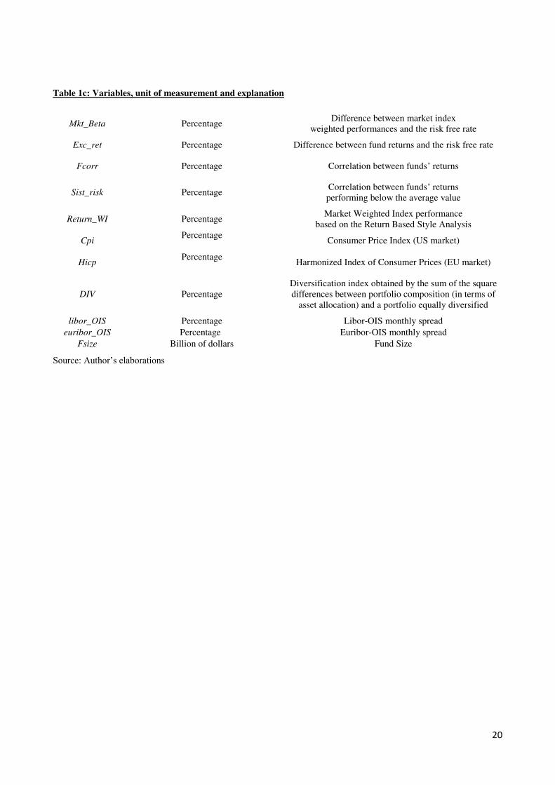
Table 1c: Variables, unit of measurement and explanation

Mkt_Beta Percentage Difference between market index

weighted performances and the risk free rate

Exc_ret Percentage Difference between fund returns and the risk free rate

Fcorr Percentage Correlation between funds‟ returns

Sist_risk Percentage Correlation between funds‟ returns

performing below the average value

Return_WI Percentage Market Weighted Index performance

based on the Return Based Style Analysis

Cpi Percentage

Consumer Price Index (US market)

Hicp Percentage

Harmonized Index of Consumer Prices (EU market)

DIV Percentage

Diversification index obtained by the sum of the square

differences between portfolio composition (in terms of

asset allocation) and a portfolio equally diversified

libor_OIS Percentage Libor-OIS monthly spread

euribor_OIS Percentage Euribor-OIS monthly spread

Fsize Billion of dollars Fund Size

Source: Author‟s elaborations

21

Table 2: CAPM model (U.S. market)

Mkt_Beta_US 1.174*** 1.177*** 1.178*** 1.150*** 1.147***

(148.00) (141.25) (140.85) (128.89) (126.16)

Syst_Risk -0.395*** -0.366*** -0.361*** -0.260*** -0.264***

(5.01) (4.51) (4.44) (3.17) (3.22)

DIV_US 0.046*** 0.044*** 0.047*** 0.047***

(3.22) (3.09) (3.31) (3.31)

Dummy 2007 0.009**

(2.01)

Dummy 2008 -0.039*** -0.038***

(8.10) (7.92)

Dummy 2009 0.008

(1.61)

Constant 0.016*** -0.003 -0.003 0.003 0.002

(10.73) (0.44) (0.55) (0.50) (0.32)

Observations 11225 10171 10171 10171 10171

R-squared 0.67 0.67 0.67 0.67 0.67

Absolute value of t statistics in parentheses.

* significant at 10%; ** significant at 5%; *** significant at 1%

Source: Author‟s elaborations

Table 3: CAPM model (EU market)

Mkt_Beta_EU 0.882*** 0.876*** 0.875*** 0.861*** 0.841***

(49.98) (47.13) (46.93) (41.56) (40.17)

Syst_Risk -0.352* -0.383* -0.388** -0.333* -0.354*

(1.83) (1.95) (1.97) (1.68) (1.79)

DIV_EU 0.026*** 0.026*** 0.028*** 0.024***

(2.12) (2.11) (2.23) (1.95)

Dummy 2007 -0.006

(0.67)

Dummy 2008 -0.018* -0.010

(1.69) (0.89)

Dummy 2009 0.051***

(5.29)

Constant -0.002 -0.015** -0.014** -0.012* -0.023***

(0.56) (2.32) (2.05) (1.84) (3.24)

Observations 3160 2770 2770 2770 2770

R-squared 0.45 0.45 0.45 0.45 0.46

Absolute value of t statistics in parentheses.

* significant at 10%; ** significant at 5%; *** significant at 1%

Source: Author‟s elaborations

22

Table 4: Simultaneous equations model (U.S. market)

First equation: Dependent variable = Market Beta

Systemic Risk -0.003*** -0.004*** -0.001*** -0.001***

(8.46) (7.67) (10.35) (14.49)

Fcorr_US -0.069*** -0.023*** -0.029*** -0.076***

(7.91) (2.77) (10.93) (20.31)

Dummy 2008 0.187*** 0.276*** 0.052*** 0.027**

(4.90) (10.10) (5.81) (2.53)

Cpi growth rate -0.031***

(7.22)

Spread Libor-OIS -0.072** -0.156***

(2.31) (22.43)

Dummy 2009 0.174*** 0.169*** 0.150***

(8.54) (27.60) (19.14)

Constant 0.136*** 0.042*** 0.052*** 0.034***

(11.11) (4.83) (20.53) (11.23)

Second Equation: Dep. Var. = Systemic Risk

Fcorr_US 16.419*** 37.284**

(4.94) (2.49)

DIV_US 0.029* 0. 030* 0.065* 0.029*

(1.27) (1.18) (0.73) (1.56)

Market Beta -1.286*** -1.431*** -1.882*** -1.688***

(4.86) (5.26) (7.23) (3.70)

Dummy 2008 49.519*** 71.096*** 38.621*** 79.826***

(6.36) (7.37) (5.97) (2.62)

Spread Libor-OIS 36.970*** 38.436***

(4.95) (4.56)

Dummy 2007 5.180***

(3.43)

Dummy 2009 45.340*** 117.786***

(5.65) (16.25)

Cpi growth rate 5.951*** 28.373*** 94.066***

(2.86) (15.82) (4.06)

Found Size 7.938*** 12.238***

(9.39) (9.68)

Constant -2.464 -15.204** -88.685*** -

402.187*** (0.75) (2.43) (11.46) (4.13)

Observations 10168 10168 10168 10168

R-Square 0.141 0.153 0.156 0.147

Absolute value of z statistics in parentheses

* significant at 10%; ** significant at 5%; *** significant at 1%

23

Table 5: Simultaneous equations model (European market)

First equation: Dependent variable = Market Beta

Systemic Risk -1.481* -1.754* -0.909*** -2.909*

(1.64) (1.44) (2.71) (1.19)

Fcorr_EU -0.117* -0.133* -0.311*** -0.04***

(1.65) (11.61) (2.78) (1.18)

Dummy 2008 0.205*** 0.074*** 0.087*** 0.196***

(12.95) (12.11) (4.05) (4.92)

HICP growth rate -0.024*** -0.025***

(7.55) (7.30)

Constant 0.189*** 0.051*** 0.108*** 0.047***

(3.99) (0.78) (14.73) (6.13)

Second equation: Dependent variable = Systemic risk

Fcorr_EU 0.079*** 0.076*** 2.311*** 0.246

(12.06) (1.40) (2.78) (9.83)

DIV_EU 0.003* 0.015* 0.008* 0.002*

(1.26) (0.35) (0.37) (0.12)

Beta_EU -0.241*** -0.241*** -0.231***

(5.47) (3.75) (3.77)

Dummy 2007 0.007* 0.012*

(0.96) (1.42)

Dummy 2008 0.106*** 0.209*** -0.217*** 0.057***

(9.65) (6.03) (4.77) (5.31)

EU spread 0.062*** 0.038*** 0.063*** 0.018*

(6.42) (3.25) (3.24) (1.40)

Dummy 2009 0.058*** 0.044

(3.75) (1.20)

Exc return EU -0.137***

(32.11)

Found Size -0.000

(0.04)

Constant -0.052*** -0.051 -0.373*** -0.115

(9.45) (7.06) (4.17) (0.89)

Observations 4484 4484 4484 4484

R-Square 0.112 0.116 0.123 0.119

Absolute value of z statistics in parentheses

* significant at 10%; ** significant at 5%; *** significant at 1%

24

Bibliography

Acharya, V., I. Hasan, and A. Saunders. “Should banks be diversified? Evidence from

individual bank loan portfolios”. Journal of Business, 79(3):1355-1412, (2006).

Acharya, V., Pedersen, L., Heje, P.T., and Richardson, M. P., “Measuring Systemic Risk”,

FRB of Cleveland Working Paper No. 10-02. Available at SSRN: http://ssrn.com/abstract=1595075

(2010).

Adrian, T., and Brunnermeier, M, K., “CoVaR”, FRB of New York Staff Report No. 348.

Available at SSRN: http://ssrn.com/abstract=1269446 (2009).

Allen, F., Gale, D., “Financial contagion”, Journal of Political Economy, (2000) 108, 1 - 33.

Allen, F., and Gale, D., “Systemic risk and regulation”. Wharton Financial Institutions

Center Working Paper No. 95-24, (2005).

Allen, F., Babus, A., Carletti, E., “Financial Connections and Systemic Risk” European

University Institute (EUI) Working Papers, ECO 2010/30 (2010).

Baele, L., De Jonghe, O., and Vennet, R. V., “Does the stock market value bank

diversification?” Journal of Banking and Finance, 31, (2007).

Bartram, S. M., Brown, G. W., and Hund J. E. “Estimating Systemic Risk in the International

Financial System”, FDIC Center for Financial Research Working Paper No. (2005).

Bartholomew, P., and Whalen, G., “Fundamentals of Systemic Risk” In Research in

Financial Services: Banking, Financial Markets, and Systemic Risk, vol.7, edited by George G.

Kaufman, 3 – 17. Greenwhich, Conn.: JAI (1995).

Berger, N., Demsetz, R., and Strahan, E., “The consolidation of financial services industry:

Causes, consequences, and implications for the future”. Journal of Banking and Finance, (23) pp.

135-194, (1999).

Bhansali, V., Gingrich, R., and Longstaff, F., “Systemic Credit Risk: What is the Market

Telling Us?”, Financial Analysts Journal 64, (4) pp. 16–24 (2008).

Bordo, D., Mizrach, M.B., and J. Schwartz, A. “Real versus pseudo-international systemic

risk: Some lessons from history”. Review of Pacific Basin Financial Markets and Policies, (1) pp.

31-58 (1998).

Campa, J.M., and Kedia S., “Explaining the diversification discount”. Journal of Finance, 57

pp. 1731-1762, (2002).

Capuano, C., “The option-ipod. The probability of default implied by option prices based on

entropy”. IMF Working Paper 08/194, 2008.

Cebenoyan S., Strahan P.E., “Risk management, capital structure and lending at banks”.

25

Journal of Banking and Finance (28) pp.19 – 43 (2004).

Chan-Lau, J. A., Mathieson, D. J., and Yao, J.Y., “Extreme contagion in equity markets”.

IMF staff paper, 51(2) pp. 386-408 (2004).

De Young, R., and Roland, K.R., “Product mix and earnings volatility at commercial banks:

Evidence from a degree of total leverage model”. Journal of Financial Intermediation, 10 pp. 54-

84, (2001).

De Vries, G.C., “Systemic risk & diversification across Euroepan banks and issuers”, Beyond

the financial crisis: systemic risk, spill over and regulation, (2010).

De Vries, G.C., Hartmann, P., and Straetmans, S., “Asset market linkages in crisis periods”.

C.E.P.R. Discussion Papers, (2001).

De Vries, C, G., “The simple economics of bank fragility”. Journal of Banking and Finance,

29(4) pp. 803-825, (2005).

De Nicolo, G., Kwast, M.L., “Systemic Risk and Financial Consolidation: Are They

Related?” Journal of Banking and Finance, Volume 26, Number 5, pp. 861-880 (2002)

De Nicolo, G., and Lucchetta, M., “Systemic Risk and the Macroeconomy,” FRB NBER

Research Conference on Quantifying Systemic Risk (2009).

De Bandt, O. and Hartmann P., “Systemic Risk: A Survey” Nov. European Central Bank

(2000).

Dow. J., “What is systemic risk? moral hazard, initial shocks, and Propagation”. Monetary

and Economic Studies, pp 1-24, (2000).

Estrella, A., “Securitization and the Efficacy of Monetary Policy”. Economic Policy Review,

Vol. 8, No. 1. Available at SSRN: http://ssrn.com/abstract=831926 (2002).

Fama, E, F., French, K.R., “The Capital Asset Pricing Model: Theory and Evidence”, Journal

of Economic Perspectives (2004), pp 25-46, N.3 (18).

Federal Reserve System Board of Governors. Technical report. n.2, (2001).

Freixas, X., Lòrànth, G., and Morrison, A., “Regulating financial conglomerates”. Oxford

Financial Research Center Working Paper no. 2005-FE-03, (2005).

Froot, K. A., & Stein, J. C., "Risk management, capital budgeting, and capital structure policy

for financial institutions: an integrated approach” Journal of Financial Economics, Elsevier, vol. 47

(1), pp. 55-82, (1998).

Giesecke, K., and Bacho, K., “Risk Analysis of Collateralized Debt Obligations”, Working

Paper (Palo Alto, California: Stanford University) Available at:

www.stanford.edu/dept/MSandE/people/faculty/giesecke/riskanalysis.pdf (2009).

Gonzlez-Hermosillo, B., Pazarbasioglu, C., and Billings, R., “Banking System Fragility:

26

Likelihood Versus Timing of Failure. An Application to the Mexican Financial Crisis,” IMF staff

paper 44,3, 295–314 (1997).

Gonzalez-Hermosillo, B., “Determinants of Ex-ante Banking System Distress: A Macro-

Micro Empirical Exploration of Some Recent Episodes” IMF Working Paper, WP/99/33 (1999).

Goodhart, C., and Segoviano, M., “Banking Stability Measures”, IMF Working Paper (2009).

Gorton, G., “Banking Panics and Business Cycles,” Oxford Economic Papers, 40, 751–781

(1998).

Greenspan, A., “Remarks at a conference on risk measurement and systemic risk”. Board of

Governors of the Federal Reserve System, Washington, D.C., 1995.

Group of Ten (G-10). “Report on consolidation in the financial sector”. Basel, (2001).

Grossman, S. R., “The shoe that didn't drop: Explaning banking stability during the great

depression”. Journal of Economic History, 54(3) pp. 654-692, (1994).

Hirtle, J., and Stiroh, K.J., The return to retail and the performance of US banks. Journal of

Banking and Finance, (21) 1101-1133, (2007).

Huang, X., Zhou, H., and Zhu, H., “Assessing the Systemic Risk of a Heterogeneous Portfolio

of Banks during the Recent Financial Crisis”. 22nd Australasian Finance and Banking Conference

2009, Available at SSRN: http://ssrn.com/abstract=1459946 (2010).

Kambhu, J., Schuermann, T., Stiroh, K.J., “Hedge Funds, Financial Intermediation, and

Systemic Risk”, Federal Reserve Bank of New York Staff Reports no. 291 (2007).

Kaufman, G.,”Comment on systemic risk”. Research in Financial Services, (1995).

Kaufman, G. G., and Scott, K. E., “What is Systemic Risk and Do Bank Regulators Retard or

Contribute to it?”, Independent Review 7, 371-391 (2003).

IMF, “Responding to the financial crisis and measuring systemic risk”. Technical report,

International Monetary Fund, (2009).

Lehar, A., “Measuring systemic risk: A risk management approach” Journal of Banking and

Finance (2005).

Lo, W. A., “Hedge Funds, Systemic Risk, and the Financial Crisis of 2007-2008”, Written

testimony prepared for the U.S House of Representatives Committee on Oversight and Government

Reform. Hearing on Hedge Funds (2008).

Longin, F., and Solnik, B., “Extreme correlation of international equity markets”. Journal of

Finance, 56(2): 649-676 (2001).

Kihlstrom, R., Romer, D., and Williams, S., “Risk Aversion with Random Initial Wealth”,

Econometrica (49) pp. 911-20 (1981).

Masera, R., Maino, R., Mazzoli, G., “Reform of the Risk Capital Standard (RCS) and

27

Systemically Important Financial Institutions (SIFIs)” in Reform of the Risk Capital Standard (Rcs)

and Systemically Important Financial Institutions (SIFIs), Bancaria Editrice (2010).

Mishkin, F., (1995) “Comment on systemic risk”, in G. Kaufman ed. Research in Financial

Services Private and Public Policy: Banking, Financial Markets and Systemic Risk. Greenwich,

Connecticut: JAI Press Inc., 7, pages 31-45 (1995).

Reichart, A.K., and Wall, L. D. “The potential for portfolio diversification in financial

services”. Federal Reserve Bank of Atlanta Economic Review, Third Quarter:31-51, (2000).

Rodriguez-Moreno, M., and Pena Sanchez de Rivera, J.I., “Systemic risk measures: the

simpler the better”. Open Access publications from Universidad Carlos III de Madrid., (2010).

Sanya, S., and Wolfe, S., “Can banks in emerging economies benefit from revenue

diversification”. Journal of Financial Services Resources (2010).

Stiroh, K., and Rumble, A., “The dark side of diversification: The case of us financial holding

companies”. Journal of Banking and Finance, 30 - 2132-2161, (2006).

Stiroh, K.J., “Do community banks benefit from diversification?” Journal of Financial

Services Resources, 25 pp. 135-160, (2004).

Stiroh, K.J., “A portfolio view of banking with interest and noninterest activities”. Journal of

Money Credit Bank, 38(5): pp. 1351–1361, (2006).

Wagner, W., “Diversification at financial institutions and systemic crises”. Journal of

Financial Intermendiation, (19) pp. 373-386 (2009).

Wheelock, D.C., “Regulation, market structure, and the bank failures of the great depression”.

Federal Reserve Bank of Saint Louis Review, 27-38, (1995).