Can the stock market be linearised?

Dimitris N. Politis∗

Department of Mathematics

University of California at San Diego

La Jolla, CA 92093-0112, USA

e-mail: dpolitis@ucsd.edu

Abstract: The evolution of financial markets is a complicated real-world phenom-

enon that ranks at the top in terms of difficulty of modeling and/or prediction.

One reason for this difficulty is the well-documented nonlinearity that is inher-

ently at work. The state-of-the-art on the nonlinear modeling of financial returns

is given by the popular ARCH (Auto-Regressive Conditional Heteroscedasticity)

models and their generalisations but they all have their short-comings. Forego-

ing the goal of finding the ‘best’ model, we propose an exploratory, model-free

approach in trying to understand this difficult type of data. In particular, we pro-

pose to transform the problem into a more manageable setting such as the setting

of linearity. The form and properties of such a transformation are given, and the

issue of one-step-ahead prediction using the new approach is explicitly addressed.

Keywords: ARCH/GARCH models, linear time series, prediction, volatility.

∗ Many thanks are due to the Economics and Statistics sections of the National Science

Foundation for their support through grants SES-04-18136 and DMS-07-06732. The au-

thor is grateful to D. Gatzouras, D. Kalligas, and D. Thomakos for helpful discussions, to

A. Berg for compiling the software for the bispectrum computations, and to R. Davis, M.

Rosenblatt, and G. Sugihara for their advice and encouragement.

1

Introduction

Consider data X1, . . . , Xn arising as an observed stretch from a financial

returns time series {Xt} such as the percentage returns of a stock index,

stock price or foreign exchange rate; the returns may be daily, weekly, or

calculated at different (discrete) intervals. The returns {Xt} are typically

assumed to be strictly stationary having mean zero which—from a practical

point of view—implies that trends and/or other nonstationarities have been

successfully removed.

At the turn of the 20th century, pioneering work of L. Bachelier [1] sug-

gested the Gaussian random walk model for (the logarithm of) stock market

prices. Because of the approximate equivalence of percentage returns to dif-

ferences in the (logarithm of the) price series, the direct implication was that

the returns series {Xt} can be modeled as independent, identically distrib-

uted (i.i.d.) random variables with Gaussian N(0, σ2) distribution. Although

Bachelier’s thesis was not so well-received by its examiners at the time, his

work served as the foundation for financial modeling for a good part of the

last century.

The Gaussian hypothesis was first challenged in the 1960s when it was

noticed that the distribution of returns seemed to have fatter tails than the

normal [14]. Recent work has empirically confirmed this fact, and has fur-

thermore suggested that the degree of heavy tails is such that the distribution

of returns has finite moments only up to order about two [12] [18] [30].

Furthermore, in an early paper of B. Mandelbrot [27] the phenomenon

of ‘volatility clustering’ was pointed out, i.e., the fact that high volatility

days are clustered together and the same is true for low volatility days; this

2

time

SP

500

retu

rns

0 500 1000 1500 2000 2500 3000

-0.2

0-0

.15

-0.1

0-0

.05

0.0

0.05

Figure 1: Daily returns of the S&P500 index spanning the period 8-30-1979

to 8-30-1991.

is effectively negating the assumption of independence of the returns in the

implication that the absolute values (or squares) of the returns are positively

correlated.

For example, Figure 1 depicts the daily returns of the S&P500 index from

August 30, 1979 to August 30, 1991; the extreme values associated with the

crash of October 1987 are very prominent in the plot. Figure 2 (a) is a ‘cor-

relogram’ of the S&P500 returns, i.e., a plot of the estimated autocorrelation

function (ACF); the plot is consistent with the hypothesis of uncorrelated

returns. By contrast, the correlogram of the squared returns of Figure 2

(b) shows some significant correlations thus lending support to the ‘volatility

clustering’ hypothesis.

The celebrated ARCH (Auto-Regressive Conditional Heteroscedasticity)

models of 2003 Nobel Laureate R. Engle [13] were designed to capture the

3

Lag

AC

F

0 10 20 30

0.0

0.2

0.4

0.6

0.8

1.0

(a) SP500 returns

Lag

AC

F

0 10 20 30

0.0

0.2

0.4

0.6

0.8

1.0

(b) SP500 returns squared

Figure 2: (a) Correlogram of the S&P500 returns. (b) Correlogram of the

S&P500 squared returns.

4

phenomenon of volatility clustering by postulating a particular structure of

dependence for the time series of squared returns {X2t }. A typical ARCH(p)

model is described by the equation1

Xt = Zt

√√√√a +

p∑i=1

aiX2t−i (1)

where a, a1, a2, . . . are nonnegative real-valued parameters, p is a nonnegative

integer indicating the ‘order’ of the model, and the series {Zt} is assumed to

be i.i.d. N(0, σ2). Bachelier’s model is a special case of the ARCH(p) model;

just let ai = 0 for all i, effectivelly implying a model of order zero.

The ARCH model (1) is closely related to an Auto-Regressive (AR) model

on the squared returns. It is a simple calculation [16] that eq. (1) implies

X2t = a +

p∑i=1

aiX2t−i + Wt (2)

where the errors Wt constitute a mean-zero, uncorrelated2 sequence. Note,

however, that the Wt’s in the above are not independent, thus making the

original eq. (1) more useful.

It is intuitive to also consider an Auto-Regressive Moving Average (ARMA)

model on the squared returns; this idea is closely related to Bollerslev’s [4]

GARCH(p, q) models. Among these, the GARCH(1,1) model is by far the

most popular, and often forms the benchmark for modeling financial returns.

The GARCH(1,1) model is described by the equation:

Xt = stZt with s2t = C + AX2

t−1 + Bs2t−1 (3)

1Eq. (1) and subsequent equations where the time variable t is left unspecified are

assumed to hold for all t = 0,±1,±2, . . . .2To talk about the second moments of Wt here, we have tacitly assumed EX4

t < ∞.

5

where the the Zts are i.i.d. N(0, 1) as in eq. (1), and the parameters A, B, C

are assumed nonnegative. Under model (3) it can be shown [4] [19] that

EX2t < ∞ only when A + B < 1; for this reason the latter is is sometimes

called a weak stationarity condition since the strict stationarity of {Xt} also

implies weak stationarity when second moments are finite.

Back-solving in the Right-Hand-Side of eq. (3), it is easy to see [19] that

the GARCH model (3) is tantamount to the ARCH model (1) with p = ∞and the following identifications:

a =C

1 − B, and ai = ABi−1 for i = 1, 2, . . . (4)

In fact, under some conditions, all GARCH(p, q) models have ARCH(∞)

representations similar to the above. So, in some sense, the only advantage

GARCH models may offer over the simpler ARCH is parsimony, i.e., achiev-

ing the same quality of model fitting with fewer parameters. Nevertheless,

if one is to impose a certain structure on the ARCH parameters, then the

effect is the same; the exponential structure (4) is a prime such example.

The above ARCH/GARCH models beautifully capture the phenomenon

of volatility clustering in simple equations at the same time implying a mar-

ginal distribution for the {Xt} returns that has heavier tails than the normal.

Viewed differently, the ARCH(p) and/or GARCH (1,1) model may be con-

sidered as attempts to ‘normalise’ the returns, i.e., to reduce the problem to a

model with normal residuals (the Zts). In that respect though the ARCH(p)

and/or GARCH (1,1) models are only partially successful as empirical work

suggests that ARCH/GARCH residuals often exhibit heavier tails than the

normal; the same is true for ARCH/GARCH spin-off models such as the

EGARCH—see [5] [40] for a review.

6

Nonetheless, the goal of normalisation is most worthwhile and it is indeed

achievable as will be shown in the sequel where the connection with the issue

of nonlinearity of stock market returns will also be brought forward.

Linear and Gaussian time series

Consider a strictly stationary time series {Yt} that—for ease of notation—is

assumed to have mean zero. The most basic tool for quantifying the inher-

ent strength of dependence is given by the autocovariance function γ(k) =

EYtYt+k and the corresponding Fourier series f(w) = (2π)−1∑∞

k=−∞ γ(k)e−iwk;

the latter function is termed the spectral density, and is well-defined (and

continuous) when∑

k |γ(k)| < ∞. We can also define the autocorrelation

function (ACF) as ρ(k) = γ(k)/γ(0). If ρ(k) = 0 for all k > 0, then the

series {Yt} is said to be a white noise, i.e., an uncorrelated sequence; the

reason for the term ‘white’ is the constancy of the resulting spectral density

function.

The ACF is the sequence of second order moments of the variables {Yt};more technically, it represents the second order cumulants [7]. The third or-

der cumulants are given by the function Γ(j, k) = EYtYt+jYt+k whose Fourier

series F (w1, w2) = (2π)−2∑∞

j=−∞∑∞

k=−∞ Γ(j, k)e−iw1j−iw2k is termed the bis-

pectral density. We can similarly define the cumulants of higher order, and

their corresponding Fourier series that constitute the so-called higher order

spectra.

The set of cumulant functions of all orders, or equivalently the set of

all higher order spectral density functions, is a complete description of the

dependence structure of the general time series {Yt}. Of course, working

7

with an infinity of functions is very cumbersome; a short-cut is desperately

needed, and presented to us by the notion of linearity.

A time series {Yt} is called linear if it satisfies an equation of the type:

Yt =∞∑

k=−∞βkZt−k (5)

where the coefficients βk are (at least) square-summable, and the series {Zt}is i.i.d. with mean zero and variance σ2 > 0. A linear time series {Yt} is

called causal if βk = 0 for k < 0, i.e., if

Yt =∞∑

k=0

βkZt−k. (6)

Eq. (6) should not be confused with the Wold decomposition that all purely

nondeterministic time series possess [20]. In the Wold decomposition the

‘error’ series {Zt} is only assumed to be a white noise and not i.i.d.; the

latter assumption is much stronger.

Linear time series are easy objects to work with since the totality of

their dependence structure is perfectly captured by a single entity, namely

the sequence of βk coefficients. To elaborate, the autocovariance and spec-

tral density of {Yt} can be calculated to be γ(k) = σ2∑∞

s=−∞ βsβs+k and

f(w) = (2π)−1σ2|β(w)|2 respectively where β(w) is the Fourier series of the

βk coefficients, i.e., β(w) =∑∞

k=−∞ βkeiwk. In addition, the bispectral den-

sity is simply given by

F (w1, w2) = (2π)−2µ3 β(−w1)β(−w2)β(w1 + w2) (7)

where µ3 = EZ3t is the 3rd moment of the errors. Similarly, all higher order

spectra can be calculated in terms of β(w).

8

The prime example of a linear time series is given by the aforementioned

Auto-Regressive (AR) family pioneered by G. Yule [45] in which the time

series {Yt} has a linear relationship with respect to its own lagged values,

namely

Yt =

p∑k=1

θkYt−k + Zt (8)

with the error process {Zt} being i.i.d. as in eq. (5). AR modeling lends itself

ideally to the problem of prediction of future values of the time series.

For concreteness, let us focus on the one-step-ahead prediction problem,

i.e., predicting the value of Yn+1 on the basis of the observed data Y1, . . . , Yn,

and denote by Yn+1 the optimal (with respect to Mean Squared Error) pre-

dictor. In general, we can write Yn+1 = gn(Y1, . . . , Yn) where gn(·) is an

appropriate function. As can easily be shown [3], the function gn(·) that

achieves this optimal prediction is given by the conditional expectation, i.e.,

Yn+1 = E(Yn+1|Y1, . . . , Yn). Thus, to implement the one-step-ahead predic-

tion in a general nonlinear setting requires knowledge (or accurate estima-

tion) of the unknown function gn(·) which is far from trivial [16] [43] [42].

In the case of a causal AR model [8] however, it is easy to show that the

function gn(·) is actually linear, and that Yn+1 =∑p

k=1 θkYn+1−k. Note fur-

thermore the property of ‘finite memory’ in that the prediction function gn(·)is only sensitive to its last p arguments. Although the ‘finite memory’ prop-

erty is specific to finite-order causal AR (and Markov) models, the linearity

of the optimal prediction function gn(·) is a property shared by all causal

linear time series satisfying eq. (6); this broad class includes all causal and

invertible, i.e., “minimum-phase” [37], ARMA models with i.i.d. innovations.

9

However, the property of linearity of the optimal prediction function gn(·)is shared by a larger class of processes. To define this class, consider a weaker

form of (6) that amounts to relaxing the i.i.d. assumption on the errors to

the assumption of a martingale difference, i.e., to assume that

Yt =∞∑i=0

βiνt−i (9)

where {νt} is a stationary martingale difference adapted to Ft, the σ-field

generated by {Ys, s ≤ t}, i.e., that

E[νt|Ft−1] = 0 and E[ν2t |Ft−1] = 1 for all t. (10)

Following [25], we will use the term weakly linear for a time series {Yt} that

satisfies (9) and (10). As it turns out, the linearity of the optimal prediction

function gn(·) is shared by all members of the family of weakly linear time

series;3 see e.g. [36] and Theorem 1.4.2 of [20].

Gaussian series form an interesting subset of the class of linear time series.

They occur when the series {Zt} of eq. (5) is i.i.d. N(0, σ2), and they too

exhibit the useful linearity of the optimal prediction function gn(·); to see

this, recall that the conditional expectation E(Yn+1|Y1, . . . , Yn) turns out to

be a linear function of Y1, . . . , Yn when the variables Y1, . . . , Yn+1 are jointly

normal [8].

Furthermore, in the Gaussian case all spectra of order higher than two are

identically zero; it follows that all dependence information is concentrated in3There exist, however, time series not belonging to the family of weakly linear series

for which the best predictor is linear. An example is given by a typical series of squared

financial returns, i.e., the series {Vt} where Vt = X2t for all t, and {Xt} is modeled by

an ARCH/GARCH model [25]. Other examples can be found in the class of random

coefficient AR models [44].

10

the spectral density f(w). Thus, the investigation of a Gaussian series’ de-

pendence structure can focus on the simple study of second order properties,

namely the ACF ρ(k) and/or the spectral density f(w). For example, an un-

correlated Gaussian series, i.e., one satisfying ρ(k) = 0 for all k, necessarily

consists of independent random variables.

To some extent, this last remark can be generalised to the linear setting: if

a linear time series is deemed to be uncorrelated, then practitioners typically

infer that it is independent as well.4 Note that to check/test whether an esti-

mated ACF, denoted by ρ(k), is significantly different from zero, the Bartlett

confidence limits are typically used—see e.g. the bands in Figure 2 (a); but

those too are only valid for linear or weakly linear time series [17] [20] [38].

To sum up: all the usual statistical goals of prediction, confidence inter-

vals and hypothesis testing are greatly facilitated in the presence of linearity,

and particularly in the presence of normality.

Linearising or normalising the stock market?

It should come as no surprise that a simple parametric model as (1) might

not perfectly capture the behavior of a complicated real-world phenomenon

such as the evolution of financial returns that—almost by definition of market

‘efficiency’—ranks at the top in terms of difficulty of modeling/prediction. As

a consequence, researchers have recently been focusing on alternative models

for financial time series.

4Strictly speaking, this inference is only valid for the aforementioned class of causal

and invertible ARMA models [6].

11

For example, consider the model

Xt = σ(t) Zt (11)

where Zt is i.i.d. (0, 1). If {σ(t)} is considered a random process independent

of {Zt}, then (11) falls in the class of stochastic volatility models [40]. If,

however, σ(·) is thought to be a deterministic function that changes slowly

(smoothly) with t, then model (11) is nonstationary—although it is locally

stationary [11]—, and σ(·) can be estimated from the data using nonpara-

metric smoothing techniques; see e.g. [21] and the references therein.

As another example, consider the nonparametric ARCH model defined

by the equation:

Xt = gp(Xt−1, . . . , Xt−p) Zt (12)

where Zt is i.i.d. (0, σ2), and gp is an unknown smooth function to be esti-

mated from the data. Additional nonparametric methods for financial time

series are discussed in the review paper [15].

Despite their nonparametric (and possibly nonstationary) character, the

above are just some different models attempting to fully capture/describe

the probabilistic characteristics of a financial time series which is perhaps an

overly ambitious task. Foregoing the goal of finding the ‘best’ model, we may

instead resort to an exploratory, model-free approach in trying to understand

this difficult type of data. In particular, we may attempt to transform the

problem into a more manageable setting such as the setting of linearity.

Consider again the financial returns data Xn = (X1, . . . , Xn), and a trans-

formation of the type Vn = H(Xn) where Vn is also n-dimensional. Ideally,

12

we would like the transformed series Vn = (V1, . . . , Vn) to be linear since, as

mentioned before, such time series are easy to work with.

However, just asking for linearity of the transformed series is not enough.

For example, the naive transformation Vt = sign(Xt) may be thought of as a

linearising transformation since, by the efficient market hypothesis, sign(Xt)

is i.i.d. (taking the values +1 and -1 with equal probability), and therefore

linear. Nevertheless, in spite of the successful linearisation, the sign trans-

formation is not at all useful as the passage from Xn to Vn is associated with

a profound loss of information.

To avoid such information loss “due to processing” [10], we should further

require that the transformation H be in some suitable sense invertible, allow-

ing us to work with the linear series Vt but then being able to recapture the

original series by the inverse transformation H−1(Vn). Interestingly, the key

to finding such a transformation is asking for more: look for a normalising

(instead of just linearising) information preserving transformation.

We now show how this quest may indeed be fruitful using the ARCH

equation (1) as a stepping stone. Note that eq. (1) can be re-written as

Zt =Xt√

a +∑p

i=1 aiX2t−i

.

Hence, we are led to define the trasformed variable Vt by

Vt =Xt√

αs2t−1 + a0X2

t +∑p

i=1 aiX2t−i

for t = p + 1, p + 2, . . . , n, (13)

and Vt = Xt/st for t = 1, 2, . . . , p. In the above, α, a0, a1, . . . , ap are non-

negative real-valued parameters, and s2t−1 is an estimator of σ2

X = V ar(X1)

based on the data up to (but not including) time t. Under the zero mean

assumption for Xt, the natural estimator is s2t−1 = (t − 1)−1

∑t−1k=1 X2

k .

13

The invertibility of the above transformation is manifested by solving

eq. (13) for Xt, thus obtaining:

Xt =Vt√

1 − a0V 2t

√√√√αs2t−1 +

p∑i=1

aiX2t−i for t = p + 1, p + 2, . . . , n. (14)

Given the initial conditions X1, . . . , Xp, the information set FXn = {Xt, 1 ≤

t ≤ n} is equivalent to the information set FVn = {Vt, 1 ≤ t ≤ n}. To

see this, note that with eq. (14) we can recursively re-generate Xt for t =

p + 1, p + 2, . . . , n using just FVn and the initial conditions; conversely, eq.

(13) defines Vt in terms of FXn .

Equation (13) describes the candidate normalising (and therefore also lin-

earising) transformation, i.e., the operator H in Vn = H(Xn); this transfor-

mation was termed ‘NoVaS’ in [31] which is an acronym for Normalizing and

Variance Stabilising. Note that formally the main difference between eq. (13)

and the ARCH eq. (1) is the presence of the term X2t paired with the coeffi-

cient a0 inside the square root; this is a small but crucial difference without

which the normalisation goal is not always feasible [29] [31]. A secondary dif-

ference is having αs2t−1 take the place of the parameter a; this is motivated

by a dimension (scaling) argument in the sense that choosing/estimating α

is invariant with respect to a change in the units of measurement of Xt. Such

invariance does not hold in estimating the parameter a in eq. (1).

Despite its similarity to model (1), eq. (13) is not to be interpreted as a

“model” for the {Xt} series. In a modeling situation, the characteristics of the

model are pre-specified (e.g., errors that are i.i.d. N(0, σ2), etc.), and standard

methods such as Maximum Likelihood or Least Squares are used to fit the

model to the data. By contrast, eq. (13) does not aspire to fully describe

14

the probabilistic behavior of the {Xt} series. The order p and the vector of

nonnegative parameters (α, a0, . . . , ap) are chosen by the practitioner with

just the normalisation goal in mind, i.e., in trying to render the transformed

series {Vt} as close to normal as possible; here, ‘closeness’ to normality can

be conveniently measured by the Shapiro-Wilk (SW) test statistic [39] or its

corresponding P -value.

It is advantageous (and parsimonious) in practice to assign a simple struc-

ture of decay for the ak coefficients. The most popular such structure—shared

by the popular GARCH(1,1) model [4]—is associated with an exponential

rate of decay, i.e., postulating that ak = Ce−dk for some positive constants

d and C which—together with the parameter α—are to be chosen by the

practitioner.

Taking into account the convexity requirement

α +∑k≥0

ak = 1,

the exponential coefficients scheme effectively has only two free parameters

that can be chosen with the normalisation goal in mind, i.e., chosen to max-

imise the SW statistic calculated on the transformed series Vt or linear com-

binations thereof—the latter in order to also ensure normality of joint distri-

butions.

As it turns out, the normalisation goal can typically be achieved by a great

number of combinations of these two free parameters, yielding an equally

great number of possible normalising transformations. Among those equally

valid normalising transformations the simplest one corresponds to the choice

α = 0. Alternatively, the value of α may be chosen by an additional op-

15

time

norm

alis

ed S

P50

0

0 500 1000 1500 2000 2500 3000

-3-2

-10

12

3

Figure 3: Normalised S&P500 returns, i.e., the tranformed V -series, spanning

the same period 8-30-1979 to 8-30-1991.

timisation criterion driven by an application of interest such as predictive

ability.

For illustration, let us revisit the S&P500 returns dataset. The normal-

ising trasformation with ak = Ce−dk and the simple choice α = 0 is achieved

with d = 0.0675; the resulting tranformed V -series is plotted in Figure 3

which should be compared to Figure 1. Not only is the phenomenon of

volatility clustering totally absent in the tranformed series but the outliers

corresponding to the crash of October 1987 are hardly (if at all) discernible.

Quantifying nonlinearity and nonnormality

There are many indications pointing to the nonlinearity of financial returns.

For instance, the fact that returns are uncorrelated but not independent is

16

a good indicator; see e.g. Figure 2 (a) and (b). Notably, the ARCH model

and its generalisations are all models for nonlinear series.

To quantify nonlinearity, it is useful to define the new function

K(w1, w2) =|F (w1, w2)|2

f(w1)f(w2)f(w1 + w2). (15)

From eq. (7), it is apparent that if the time series is linear, then K(w1, w2)

is the constant function—equal to µ23/(2πσ6) for all w1, w2; this observation

can be used in order to test a time series for linearity [22] [41]; see also [23]

[24] and [26] for an up-to-date review of different tests for linearity.5 In the

Gaussian case we have µ3 = 0 and therefore F (w1, w2) = 0 and K(w1, w2) = 0

as well.

Let K(w1, w2) denote a data-based nonparametric estimator of the quan-

tity K(w1, w2). For our purposes, K(w1, w2) will be a kernel smoothed esti-

mator based on infinite-order flat-top kernels that lead to improved accuracy

[33]. Figure 4 shows a plot of K(w1, w2) for the S&P500 returns; its non-

constancy is direct evidence of nonlinearity. By contrast, Figure 5 shows

a plot of K(w1, w2) for the normalised S&P500 returns, i.e., the V -series.

Note that, in order to show some nontrivial pattern, the scale on the vertical

axis of Figure 5 is 500 times bigger than that of Figure 4. Consequently, the

function K(w1, w2) for the normalised S&P500 returns is not statistically dif-

ferent from the zero function, lending support to the fact that the trasformed

series is linear with distribution symmetric about zero; the normal is such a

distribution but it is not the only one.

5A different—but related—fact is that the closure of the class of linear time series is

large enough so that it contains some elements that can be confused with a particular type

of nonlinear time series; see e.g. Fact 3 of [2].

17

Figure 4: ABOUT HERE

Figure 5: ABOUT HERE

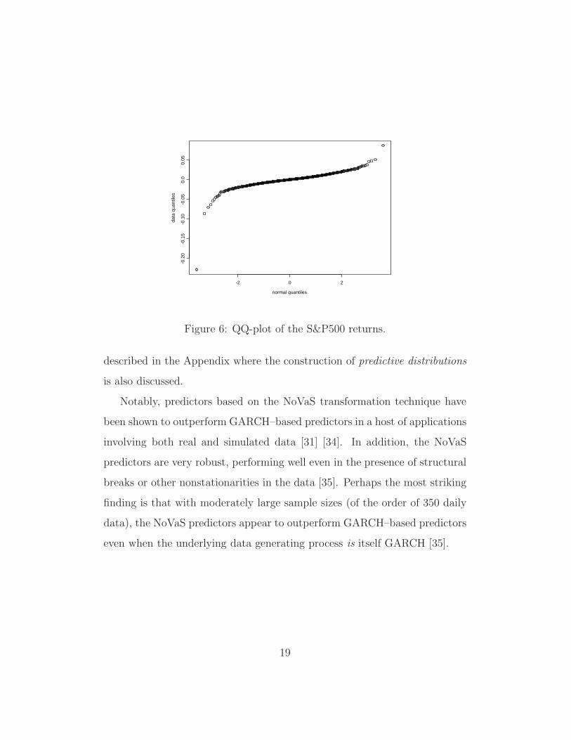
To further delve into the issue of normality, recall the aforementioned

Shapiro-Wilk (SW) test which effectively measures the lack-of-fit of a quantile-

quantile plot (QQ-plot) to a straight line. Figure 6 shows the QQ-plot of the

S&P500 returns; it is apparent that a straight line is not a good fit. As

a matter of fact the SW test yields a P-value that is zero to several dec-

imal points—the strongest evidence of nonnormality of stock returns. By

contrast, the QQ-plot of the normalised S&P500 returns can be very well

approximated by a straight line: the R2 associated with the plot in Figure 7

is 0.9992, and the SW test yields a P-value of 0.153 lending strong support to

the fact that the trasformed series is indistiguishable from a Gaussian series.

The proposed transformation technique has been applied to a host of dif-

ferent financial datasets including returns from several stock indices, stock

prices and foreign exchange rates [34]. Invariably, it was shown to be suc-

cessful in its dual goal of normalisation and linearisation. Furthermore, as al-

ready discussed, a welcome by-product of linearisation/normalisation is that

the construction of out-of-sample predictors becomes easy in the transformed

space.

Of course, the desirable objective is to obtain predictions in the original

(untransformed) space of financial returns. The first thing that comes to

mind is to invert the transformation so that the predictor in the transformed

space is mapped back to a predictor in the original space; this is indeed pos-

sible albeit suboptimal. Optimal predictors were formulated in [31], and are

18

normal quantiles

data

qua

ntile

s

-2 0 2

-0.2

0-0

.15

-0.1

0-0

.05

0.0

0.05

Figure 6: QQ-plot of the S&P500 returns.

described in the Appendix where the construction of predictive distributions

is also discussed.

Notably, predictors based on the NoVaS transformation technique have

been shown to outperform GARCH–based predictors in a host of applications

involving both real and simulated data [31] [34]. In addition, the NoVaS

predictors are very robust, performing well even in the presence of structural

breaks or other nonstationarities in the data [35]. Perhaps the most striking

finding is that with moderately large sample sizes (of the order of 350 daily

data), the NoVaS predictors appear to outperform GARCH–based predictors

even when the underlying data generating process is itself GARCH [35].

19

normal quantiles

data

qua

ntile

s

-2 0 2

-3-2

-10

12

3

Figure 7: QQ-plot of the normalised S&P500 returns.

Appendix: Prediction via the transformation technique

For concreteness, we focus on the problem of one-step ahead prediction, i.e.,

prediction of a function of the unobserved return Xn+1, say h(Xn+1), based

on the observed data FXn = {Xt, 1 ≤ t ≤ n}. Our normalising transformation

affords us the opportunity to carry out the prediction in the V -domain where

the prediction problem is easiest since the problem of optimal prediction

reduces to linear prediction in a Gaussian setting.

The prediction algorithm is outlined as follows:

• Calculate the transformed series V1, . . . , Vn using eq. (13).

• Calculate the optimal predictor of Vn+1, denoted by Vn+1, given FVn .

This predictor would have the general form Vn+1 =∑q−1

i=0 ciVn−i. The

ci coefficients can be found by Hilbert space projection techniques, or

20

by simply fitting the causal AR model

Vt+1 =

q−1∑i=0

ciVt−i + εt+1. (16)

to the data where εt is i.i.d. N(0, σ2). The order q can be chosen by

an information criterion such as AIC or BIC [9].

Note that eq. (14) suggests that h(Xn+1) = un(Vn+1) where un is given by

un(V ) = h

⎛⎝ V√

1 − a0V 2

√√√√αs2t−1 +

p∑i=1

aiX2n+1−i

⎞⎠ .

Thus, a quick-and-easy predictor of h(Xn+1) could then be given by un(Vn+1).

A better predictor, however, is given by the center of location of the dis-

tribution of un(Vn+1) conditionally on FVn . Formally, to obtain an optimal

predictor, the optimality criterion must first be specified, and correspond-

ingly the form of the predictor is obtained based on the distribution of the

quantity in question. Typical optimality criteria are L2, L1 and 0/1 losses

with corresponding optimal predictors the (conditional) mean, median and

mode of the distribution. For reasons of robustness, let us focus on the

median of the distribution of un(Vn+1) as such a center of location.

Using eq. (16) it follows that the distribution of Vn+1 conditionally on FVn

is approximately N(Vn+1, σ2) where σ2 is an estimate of σ2 in (16). Thus,

the median-optimal one-step-ahead predictor of h(Xn+1) is the median of

the distribution of un(V ) where V has the normal distribution N(Vn+1, σ2)

truncated to the values ±1/√

a0; this median is easily computable by Monte-

Carlo simulation.

The above Monte-Carlo simulation actually creates a predictive distrib-

ution for the quantity h(Xn+1). Thus, we can go a step further from the

21

notion of a point-predictor: clipping the left and right tail of this predictive

distribution, say δ·100% on each side, a (1 − 2δ)100% prediction interval

for h(Xn+1) is obtained. Note, however, that this prediction interval treats

as negligible the variability of the fitted parameters α, a0, a1, ..., ap which is

a reasonable first-order approximation; alternatively, a bootstrap method

might be in order [28] [32].

References

[1] Bachelier, L. (1900). Theory of Speculation. Reprinted in: The Random

Character of Stock Market Prices, P.H. Cootner (Ed.), MIT Press,

Cambridge, Mass., pp. 17-78, 1964.

[2] Bickel, P. and Buhlmann, P. (1997). Closure of Linear Processes. J.

Theor. Prob., 10, 445-479.

[3] Billingsley, P. (1986). Probability and Measure, 2nd ed. John Wiley, New

York.

[4] Bollerslev, T. (1986). Generalized autoregressive conditional het-

eroscedasticity, J. Econometrics, 31, 307-327.

[5] Bollerslev, T., Chou, R. and Kroner, K. (1992). ARCH modeling in

finance: a review of theory and empirical evidence, J. Econometrics, 52,

5-60.

22

[6] Breidt, F.J., Davis, R.A. and Trindade, A.A. (2001). Least absolute

deviation estimation for all-pass time series models, Annals of Statistics,

29, pp. 919-946.

[7] Brillinger, D. (1975). Time Series: Data Analysis and Theory. Holt,

Rinehart and Winston, New York.

[8] Brockwell, P. and Davis, R. (1991). Time Series: Theory and Methods,

2nd ed. Springer, New York.

[9] Choi, B.S. (1992), ARMA Model Identification, Springer, New York.

[10] Cover, T. and Thomas, J. (1991). Elements of Information Theory, John

Wiley, New York.

[11] Dahlhaus, R. (1997). Fitting time series models to nonstationary

processes, Annals of Statistics, 25, 1-37.

[12] Davis, R. A., and Mikosch, T. (2000). The sample autocorrelations

of financial time series models. In Nonlinear and nonstationary signal

processing, pp. 247–274, Cambridge Univ. Press, Cambridge.

[13] Engle, R. (1982). Autoregressive conditional heteroscedasticity with es-

timates of the variance of UK inflation, Econometrica, 50, 987-1008.

[14] Fama, E.F. (1965). The behaviour of stock market prices, J. Business,

38, 34-105.

[15] Fan, J. (2005). A selective overview of nonparametric methods in finan-

cial econometrics, Statist. Sci., vol. 20, no. 4.

23

[16] Fan, J. and Yao, Q. (2003). Nonlinear Time Series, Springer, New York.

[17] Fuller, W.A. (1996). Introduction to Statistical Time Series, 2nd Ed.,

John Wiley, New York.

[18] Gabaix, X., Gopikrishnan, P., Plerou, V. and Stanley, H.E. (2003). A

theory of power-law distributions in financial market fluctuations, Na-

ture, vol. 423, 267-270.

[19] Gourieroux, C. (1997). ARCH Models and Financial Applications,

Springer, New York.

[20] Hannan, E.J. and Deistler, M. (1988). The Statistical Theory of Linear

Systems, John Wiley, New York.

[21] Herzel, S., Starica, C., and Tutuncu, R. (2006). A non-stationary para-

digm for the dynamics of multivariate returns. In Dependence in Prob-

ability and Statistics, (P. Bertail, P. Doukhan, and P. Soulier, Eds.),

Springer Lecture Notes in Statistics No. 187, Springer, New York, pp.

391–430.

[22] Hinich, M.J. (1982). Testing for Gaussianity and linearity of a stationary

time series, J. Time Ser. Anal., vol. 3, no. 3, 169-176.

[23] Hinich, M.J. and Patterson, D.M. (1985). Evidence of nonlinearity in

stock returns, J. Bus. Econ. Statist., 3, pp. 69-77.

[24] Hsieh, D. (1989). Testing for nonlinear dependence in daily foreign ex-

change rates, J. Business, 62, pp. 339-368.

24

[25] Kokoszka, P. and Politis, D. N. (2008). The variance of sample au-

tocorrelations: does Bartlett’s formula work with ARCH data?, Dis-

cussion paper no. 2008-12, Dept. of Economics, UCSD; available at:

http://repositories.cdlib.org/ucsdecon/2008-12.

[26] Kugiumtzis, D. (2008). Evaluation of surrogate and boot-

strap tests for nonlinearity in time series, Studies in Non-

linear Dynamics and Econometrics, vol. 12, no. 1, article 4.

[http://www.bepress.com/snde/vol12/iss1/art4].

[27] Mandelbrot, B. (1963). The variation of certain speculative prices, J.

Business, 36, 394-419.

[28] Politis, D. N. (2003a). The impact of bootstrap methods on time series

analysis, Statistical Science, Vol. 18, No. 2, 219-230.

[29] Politis, D.N. (2003b). A normalizing and variance-stabilizing transfor-

mation for financial time series, in Recent Advances and Trends in Non-

parametric Statistics, (M.G. Akritas and D.N. Politis, Eds.), Elsevier

(North Holland), pp. 335-347.

[30] Politis, D. N. (2004). A heavy-tailed distribution for ARCH residuals

with application to volatility prediction, Annals Econ. Finance, vol. 5,

pp. 283-298.

[31] Politis, D. N. (2007). Model-free vs. model-based volatility prediction,

J. Financial Econometrics, vol. 5, no. 3, pp. 358-389, 2007.

25

[32] Politis, D. N. (2008). Model-free model-fitting and predictive distribu-

tions, Discussion paper no. 2008-14, Dept. of Economics, UCSD; avail-

able at: http://repositories.cdlib.org/ucsdecon/2008-14.

[33] Politis, D. N., and Romano, J.P. (1995). Bias-Corrected Nonparametric

Spectral Estimation, J. Time Ser. Anal., 16, 67-104.

[34] Politis, D. N. and Thomakos, D. D. (2008). Financial Time Series and

Volatility Prediction using NoVaS Transformations, in Forecasting in the

Presence of Parameter Uncertainty and Structural Breaks, D. E. Rapach

and M. E. Wohar (Eds.), Emerald Group Publishing Ltd. (United King-

dom), pp. 417–447.

[35] Politis, D. N. and Thomakos, D. D. (2008). NoVaS Transfor-

mations: Flexible Inference for Volatility Forecasting, Discussion

paper no. 2008-13, Dept. of Economics, UCSD; available at:

http://repositories.cdlib.org/ucsdecon/2008-13.

[36] Poskitt, D.S. (2008). Properties of the sieve bootstrap for fractionally

integrated and non-invertible processes, J. Time Ser. Anal., vol. 29, no.

2, pp. 224-250.

[37] Rosenblatt, M. (2000), Gaussian and Non-Gaussian Linear Time Series

and Random Fields, Springer, New York.

[38] Romano, J.P. and Thombs, L. (1996). Inference for Autocorrelations

under Weak Assumptions, J. Amer. Statist. Assoc., 91, 590-600.

[39] Shapiro, S.S. and Wilk, M. (1965). An analysis of variance test for nor-

mality (complete samples), Biometrika, Vol. 52, 591-611.

26

[40] Shephard, N. (1996). Statistical aspects of ARCH and stochastic volatil-

ity. in Time Series Models in Econometrics, Finance and Other Fields,

D.R. Cox, David V. Hinkley and Ole E. Barndorff-Nielsen (eds.), Lon-

don: Chapman & Hall, pp. 1-67.

[41] Subba Rao, T. and Gabr, M. (1984). An Introduction to Bispectral

Analysis and Bilinear Time Series Models, Springer Lecture Notes in

Statistics No. 24, New York.

[42] Sugihara, G. and May, R.M. (1990). Nonlinear forecasting as a way of

distinguishing chaos from measurement error in time series, Nature, vol.

344, 734-741.

[43] Tong, H. (1990). Non-linear Time Series Analysis: a Dynamical Systems

Approach, Oxford Univ. Press, Oxford.

[44] Tsay, R.S. (2002). Analysis of Financial Time Series, Wiley, New York.

[45] Yule, G.U. (1927). On a method of investigating periodicities in dis-

turbed series with special reference to Wolfer’s sunspot numbers, Phil.

Trans. Roy. Soc. (London) A, 226, 267-298.

27

Figure 4: Plot of K(ω1, ω2) vs. (ω1, ω2) for the S&P500 returns.

Figure 5: Plot of K(ω1, ω2) vs. (ω1, ω2) for the normalized S&P500 returns.

1