canadian society ofagricultural engineering · canadian society ofagricultural engineering an...
TRANSCRIPT

A
Paoer No.
AN ASAE;CSAE MEH71NG
PRESENTATION
Canadian Society
of Agricultural
EngineeringAN APPROXIMATE OVERLAND FLOW
ROOTING MODEL
M. Hernandez
Research Assiscane
University of Arizona
Tucson, AZ 85721
USA
By
L.J. Lane
Research Hydrologist
USDA-ARS
2000 E. Allen Road
Tucson, AZ 85719
USA
J.J. Scone
Research Assiscanc
University of Arizona
Tucson, AZ 85721
USA
Written for presentation at the 1989
International Summer Meeting jointly
sponsored by the AMERICAN SOCIETY OF
AGRICULTURAL ENGINEERS and the CANADIAN
SOCIETY OF AGRICULTURAL ENGINEERING
Quebec Municipal Convention Centre
Quebec, PQ, Canada
June 25-28, 1989
SUMMARY: ^g approximate overland flow routing
method estimated peak runoff and duration of
runoff accurately when disaggregated rainfall
intensity was input to generate the rainfall
excess distribution.
American
Scdety
of Agricultural
Engineers
KEYWORDS:
Hydrology, rainfall, runoff, watersheds
This is an original presentation ot tna autnons) vtno alone are rasoonsiale for its
contents.
The Soaetv is not resoonstale (or statements or ooinions advanced in reoorts or
exoressea at its meetings, fleoorts are not suoieet to trie (ormat oaer review oracess
by ASAE editorial committees: ttiareiore. are not to Do raoresemeo as retareea
puaiications.
Heoorts at presentations mada at ASAE meeiinqs are considered to 08 tne orooartv
at tna Society. Quotation (ram (fits work snoutd state tnat it is >rom a presentation
made oy (tna auinora at the (listeot ASAE meeting.
St. Joseph, Ml 49085-9659 USA

Abstract
The Water Erosion Prediction Project (WEPP), under the leadership of che
Agricultural Research Service, is to develop a physical process model of
soil loss and sediment yield for croplands and rangelands. Hydrologically,
the model includes a rainfall disaggregation scheme, the Green and Ampt
infiltration equation, and two methods of routing rainfall excess based on
the kinematic wave equations and the approximate overland flow routing
method. The purpose of this paper is to describe the second method to route
the excess rainfall. The approximate overland flow routing method wasdeveloped based on the assumption that: the routed overland flow hydrograph
may be well approximated by the rainfall excess distribution. The method
consists of a set of regression equations derived using the method ofcharacteristic solution for the rising hydrograph. The method estimates
peak runoff and duration of runoff based on plane characteristics and
rainfall excess pattern. To assess the approximate routing method, data
from three small watersheds were used to obtain peak runoff and duration ofrunoff using an analytical solution to the kinematic wave equations.
Comparison between the approximate method and kinematic routing agreed
within 5% error.
Introduction
The WEPP is developing new generation erosion prediction technology fordealing with soil conservation and environmental problems resulting fromsoil erosion by water. The model structure of WEPP is based on fundamental
hydrologic and erosion processes. The model structure includes: climate,
snow accumulation, infiltration, runoff, erosion, crop growth, plant residue
and other soil disturbing activities. The WEPP Model uses the steady state
sediment continuity equation as a basis for erosion computation. To solve ■
the steady state sediment continuity equation one requires the peak runoff, ""
duration of runoff and flow shear stress. The first two hydrologic
variables are obtained by routing the rainfall excess along the overlandflow plane. Overland flow has been modeled in the past using the one-
dimensional kinematic wave approximation (Henderson and Wooding 1964,Liggett and Woolhiser 1967, Woolhiser and Liggett 1967, Eagleson 1970).
Finite difference methods- have been used to solve the one-dimensional
kinematic wave equations• with the resultant increase in computer time. The
approximate routing method, which will be described in the next section,
provides the peak runoff and duration of runoff without resorting to finite
difference methods.
The kinematic wave equations for one-dimensional overland flow result when
the momentum equation is approximated by assuming the land slope, So, is
equal to the friction slope, Sf. The kinematic wave equations for runoff on
a plane are
|* + fa _ r _ f _ v (l)at 3x

and
q - a
where h is the local, depth of flow (m), t is the time (s) , q is the
discharge per unit width (m/s) , x is the distance down the plane (m), r is
the rainfall intensity (m/s), f is the infiltration rate (m/s), v is the
rainfall excess rate (m/s), and a is the depth-discharge coefficient
(m^ /s) . If v in equation (1) is constant, then equations (1) and (2) canbe solved analytically by che method of characteristics (Eagleson 1970) .
Analytic solutions to these equations have been derived for the case where v
is made up of a series of step functions in the rainfall intensity pattern,
i.e. where intensity is constant within an arbitrary time interval but
varies from interval to interval (Shirley 1987).
Development of the Approximate Flow Routing Method
Let the duration of rainfall excess, Dv, be defined as the time from the
first time to ponding to the last time during the storm when rainfall rate
is greater than the calculated infiltration capacity. Let the volume of
rainfall excess be V. Therefore, we can define an average rainfall excess
rate, a as
° " it (3)Dv
where a is the average rate of rainfall excess (m/s), V is the volume of
rainfall excess (m), and Dv duration of rainfall excess (s). If the time to
equilibrium, te, for runoff on a plane of length x is the time to steady
state runoff given an average rainfall excess rate, a , for a long period,
then the time to equilibrium is calculated as follows (Eagleson 1970).
te -
where x is the length of the plane (m), te is the time to equilibrium (s).
Having characterized the rainfall excess pattern and the overland flow
plane, it is now possible to define the dimensionless variables used to
approximate the peak rate of runoff and the duration of runoff without doing
the actual routing process. Let the normalized time to equilibrium, t*, be
c* - -^ (5)Dv
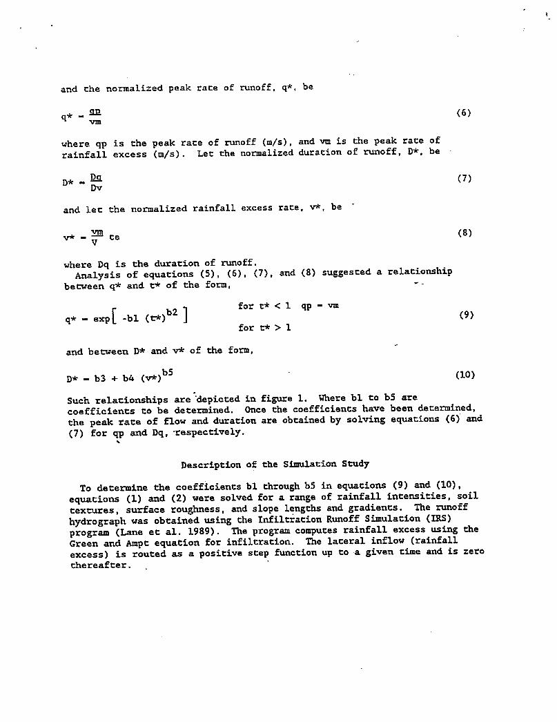
and Che normalized peak race of runoff, q*. be
* - SB.^ vm
where qp is Che peak race of runoff (m/s), and vm is Che peak race of
rainfall excess (m/s). Lee che normalized duracion of runoff, D*. be
■>* - % a)
and lee Che normalized rainfall excess race, v*. be
v* - f ce
where Dq is Che duracion of runoff.Analysis of equaCions (5), (6), (7), and (8) suggesced a relaCionship
becween q* and C* of Che form,
- for C* < 1 qp - vm
q* - exp[ -bl (C*)b2 ]for c* > 1
and becween D* and v* of Che form,
D* - b3 + b4 (v*)b5
Such relacionships are depicced in figure 1. Where bl Co b5 are
coefficiencs Co be decermined. Once Che coefficiencs have been decermined,
che peak race of flow and duracion are obcained by solving equaCions (6) and
(7) for qp and Dq, -respectively.
Descripcion of che Simulacion SCudy
To decermine Che coefficiencs bl chrough b5 in equaCions (9) and (10),
equaCions (1) and (2) were solved for a range of rainfall incensicies, soil
cexcures, surface roughness, and slope lengchs and gradiencs. The runoff
hydrograph was obcained using Che InfilCracion Runoff Simulacion (IRS)
program (Lane eC al. 1989). The program compuces rainfall excess using che
Green and AmpC equaCion for infilcracion. The laceral inflow (rainfall
excess) is rouCed as a posicive sCep funccion up Co a given Cime and is zero
chereafcer.
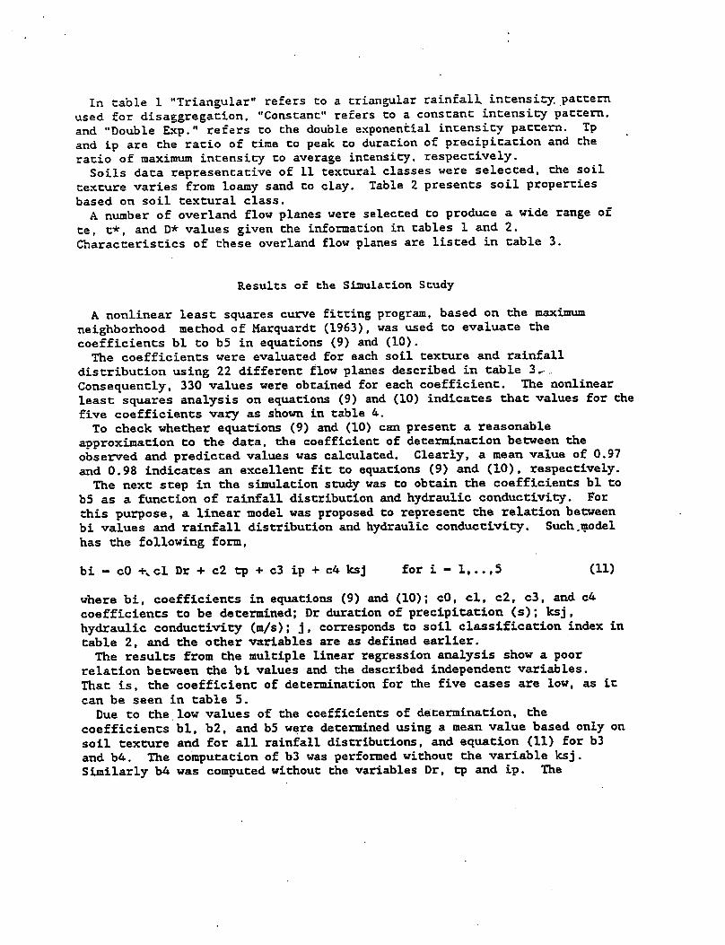
In table 1 "Triangular" refers Co a triangular rainfall intensity, pattern
used for disaggregation. "Constant" refers to a constant intensity pattern,
and "Double Exp." refers to the double exponential intensity pattern. Tp
and ip are the ratio of time to peak to duration of precipitation and the
ratio of maximum intensity to average intensity, respectively.
Soils data representative of 11 textural classes were selected, the soil
texture varies from loamy sand to clay. Table 2 presents soil properties
based on soil textural class.
A number of overland flow planes were selected to produce a wide range of
te, t*, and D* values given the information in tables 1 and 2.
Characteristics of these overland flow planes are listed in table 3.
Results o£ the Simulation Study
A nonlinear least squares curve fitting program, based on the maximum
neighborhood method of Marquardt (1963), was used to evaluate the
coefficients bl to b5 in equations (9) and (10).
The coefficients were evaluated for each soil texture and rainfall
distribution using 22 different flow planes described in table 3^.
Consequently, 330 values were obtained for each coefficient. The nonlinear
least squares analysis on equations (9) and (10) indicates that values for the
five coefficients vary as shown in table 4.
To check whether equations (9) and (10) can present a reasonable
approximation to the data, the coefficient of determination between the
observed and predicted values was calculated. Clearly, a mean value of 0.97
and 0.98 indicates an excellent fit to equations (9) and (10), respectively.
The next step in the simulation study was to obtain the coefficients bl to
b5 as a function of rainfall distribution and hydraulic conductivity. For
this purpose, a linear model was proposed to represent the relation between
bi values and rainfall distribution and hydraulic conductivity. Such .model
has the following form,
bi - cO H\ cl Dr + c2 tp + c3 ip + c4 ksj for i - 1,.. ,5 (11)
where bi, coefficients in equations (9) and (10); cO, cl, c2, c3, and c4
coefficients to be determined; Dr duration of precipitation (s); ksj ,
hydraulic conductivity (ta/s); j, corresponds to soil classification index in
table 2, and the other variables are as defined earlier.
The results from the multiple linear regression analysis show a poor
relation between the bi values and the described independent variables.
That is, the coefficient of determination for the five cases are low, as it
can be seen in table 5.
Due to the low values of the coefficients of determination, the
coefficients bl, b2, and b5 were determined using a mean value based only on
soil texture and for all rainfall distributions, and equation (11) for b3
and b4. The computation of b3 was performed without the variable ksj.
Similarly b4 was computed without the variables Dr, tp and ip. The

regression analysis showed that such variables did not reduce Che
unexplained variance significantly. Three sees of eleven mean values were
generated, see table 6.
Similarly, a mean value was computed for each coefficient for a given
rainfall distribution and for all soil textures. Consequently, three sets
of thirty mean values were produced, see table 7.
Further simplification was made to values of the coefficients in tables 6
and 7. The criterion for such simplification was based only on soil
texture. Table 8 shows the values of bl, b2, and b5 for different soil
textures.
In contrast, b3 was determined using equation (11) for each soil texture.
Thus a set of eleven equations were obtained to calculate b3. For instance
table 9 shows the values of the coefficients in equation (11) for all soil
textures.
Similarly, b4 can be determined as
b4 - 0.47 + 5.55E-03 ksj (12)
Application and Discussion
Infiltration-based runoff estimation procedures require rainfall time-
intensity data. However, often times only storm total or daily rainfall
data are available. Therefore Nicks and Lane (1989) developed a
disaggregation scheme to develop approximate rainfall intensity patterns
using information on rainfall intensity amount, storm duration, time to peak
rainfall intensity, and maximum rainfall intensity within the storm. In
this section we evaluate the approximate method versus kinematic routing for
observed rainfall intensity patterns and for approximate rainfall intensity
patterns produced by the disaggregation scheme.
The approximate routing method was tested using data from three small
watersheds. The following information was provided for the three
watersheds: observed rainfall data and disaggregated rainfall data, see
figures 2xto 6, slope and length of the plane, ground and canopy cover,
initial saturation and Chezy roughness coefficient. Table 10 presents
watershed characteristics at the time of the storms.
Results for the .5 events are shown in tables 11 and 12. The data in
Table 11 show how well the approximate method agrees with kinematic routing
when measured rainfall data are used as input. The data in Table 12 show
the corresponding information when the disaggregated rainfall data are used
as input.
Summary
The WEPP Model uses the approximate routing method to obtain peak runoff
and duration of runoff since a rainfall disaggregation scheme (Nicks and
Lane 1989) was developed in the model to calculate rainfall statistics such

as amount, duration, cirae Co peak incensity and maximum rainfall incensicy.
These statistics are used to fit a double exponential distribution to a
normalized intensity pattern. The Green and Ampc equation computes
infiltration and rainfall excess as a function of this normalized intensity
pattern.
The approximate overland flow routing mechod estimated peak runoff and
duration of runoff accurately when disaggregated rainfall intensity was
input to generate the rainfall excess distribution. Tables 11 and 12 show
values for peak runoff and duration of runoff for the three small
watersheds. When observed data were input estimated values were
unsatisfactory, see table 11. Notice that all storms except 7/19/68 in
table 11 have an irregular intensity pattern, figures 2, 3, 5, and 6.
Conversely, storm 7/19/68, figure 4, shows a more regular pattern.
Consequently, difference between kinematic routing and approximate method is
small. In addition, storm 7/19/68 shows a similar pattern to the
disaggregated storm, figure 4. When disaggregated rainfall intensity data
were input the approximate method agrees with the routing values. Notice
that all disaggregated rainfall intensity distributions show no abrupt
discontinuities, figures 2-6. The disaggregation process smooths out the
observed rainfall intensity pattern.
The approximate routing method was developed based on the assumption that
the routed overland flow hydrograph may be well approximated by the rainfall
excess distribution. As a result, peak runoff and duration of runoff were
calculated accurately when the rainfall excess distribution was generated
from a disaggregated rainfall intensity pattern. For instance, figure 7
shows rainfall excess distributions obtained from storm 3/19/70. Clearly,
the rainfall excess distribution from observed rainfall intensity shows more
discontinuities than the one obtained from disaggregated intensity, figure
7.
References
Eagleson.^P. S. 1970. Dynamic Hydrology. McGraw-Hill Book Co., New York,
462.
Henderson, F. M. and R. A. Wooding. 1964. Overland flow and groundwater
flow from a steady rainfall of finite duration. J. Geophys. Res.
69(8):1531-1540.
Liggett, J. A. and D. A. Woolhiser. 1967. The use of the shallow water
equations in runoff computation, p. 117-126. In: Proc. Third Annual Amer.
Water Resources Conf., AWRA, San Francisco, CA,
Lane, L. J., E. D. Shirley, and J. J. Stone. 1988. Program IRS.
Unpublished documentation for computer program. USDA-ARS, Tucson, AZ.

Marquardt, D. W. 1963. An algorichm for lease squares estimation of
nonlinear parameters. J. Soc. Ind. Appl. Math. 11:431-441.
Nicks, A. D., and L. J. Lane. 1989.' Chapcer 2. Weanher Generacor. WEPP
Profile Model Documencacion, USDA-ARS, Tucson, AZ.
Shirley, E. D. 1987. Program HDRIVER. Unpublished documencacion for
computer program. USDA-ARS, Tucson, AZ.
Woolhiser, D. A. and J. A. Liggecc. 1967. Unsceady, one-dimensional flow
over a plane Che rising hydrograph. Wacer Resources Res. 3(3):753-771.
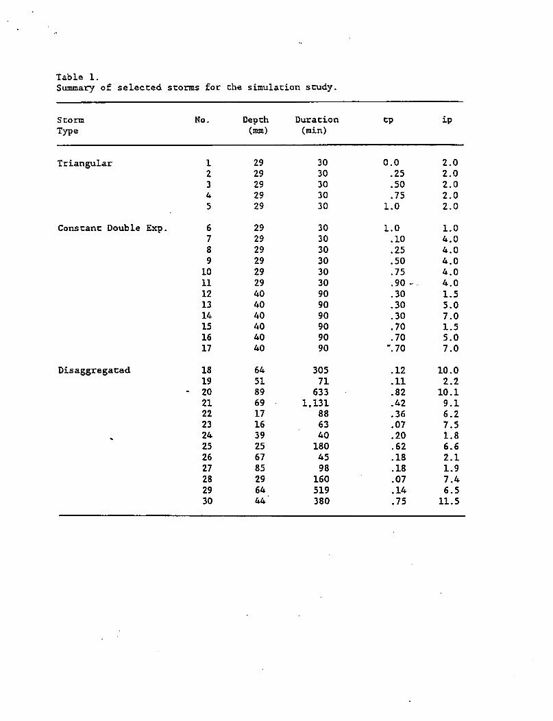
Table 1.
Summary of selected storms for the simulation study.
Storm
Type
No. Depth
(mm)
Duration
(rain)
tp
Triangular
Constant Double Exp.
Disaggregated
1
2
3
4
5
6
7
8
9
10
11
12
13
14
15
16
17
18
19
20
21
22
23
24
25
26
27
28
29
30
29
29
29
29
29
29
29
29
29
29
29
40
40
40
40
40
40
64
51
89
69
17
16
39
25
67
85
29
64
44
30
30
30
30
30
30
30
30
30
30
30
90
90
90
90
90
90
305
71
633
1,131
88
63
40
180
45
98
160
519
380
0.0
.25
.50
.75
1.0
1.0
.10
.25
.50
.75
.90 -..
.30
.30
.30
.70
.70
".70
.12
.11
.82
.42
.36
.07
.20
.62
.18
.18
.07
.14
.75
2.0
2.0
2.0
2.0
2.0
1.0
4.0
4.0
4.0
4.0
4.0
1.5
5.0
7.0
1.5
5.0
7.0
10.0
2.2
10.1
9.1
6.2
7.5
1.8
6.6
2.1
1.9
7.4
6.5
11.5
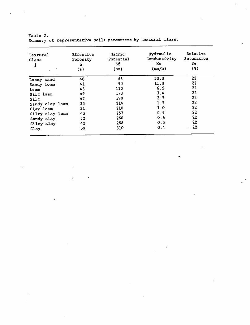
Table 2.
Summary of represencacive soils parameters by cexcural class.
Texcural
Class
j
Loamy sand
Sandy loam
Loam
Silc loam
Silc
Sandy clay loam
Clay loam
Silty clay loam
Sandy clay
Silty clay
Clay
Effeccive
Porosicy
n
(%)
40
41
43
49
42
35
31
43
32
42
39
Macric
PoCencial
Sf
(mm)
63
90
110
173
190
214
210
253
260
288
310
Hydraulic
Conduceivicy
Ks
(nun/h)
30.0
11.0
6.5
3.4
2.5
1.5
1.0
0.9
0.6
0.5
0.4
Relative
Sacuracion
Se
(%)
22
22
22
22
22
22
22
22
22
22
- 22
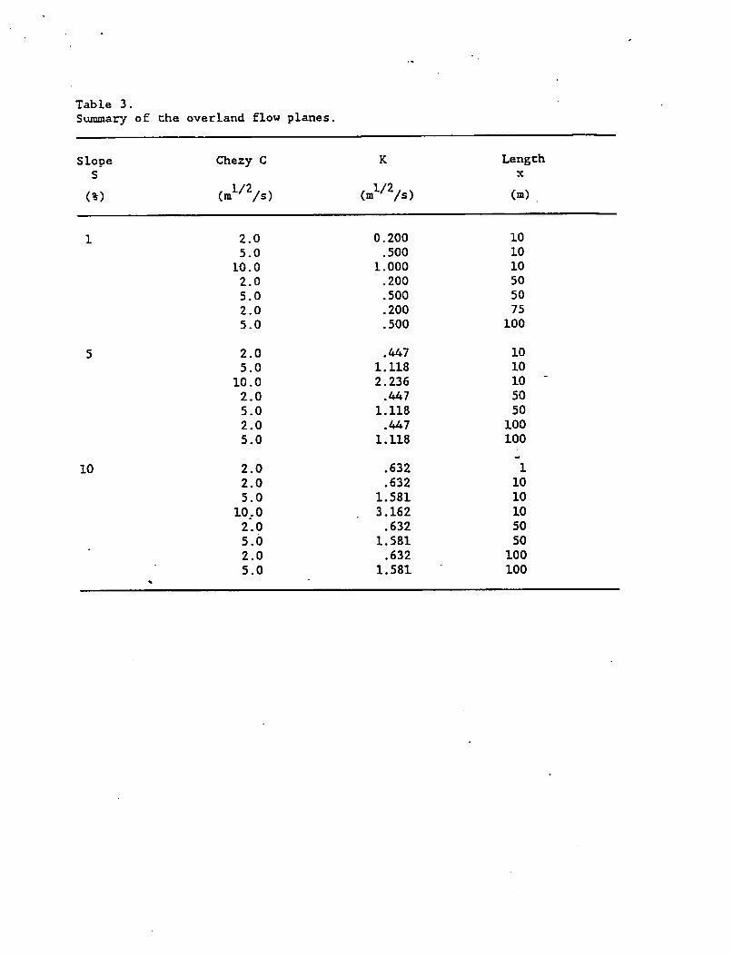
Table 3.
Summary of che overland flow planes.
Slope Chezy C K Length
S x
(m1/2/s) (m^Vs) (m)
1 2.0
5.0
10.0
2.0
5.0
2.0
5.0
5 2.0
5.0
10.0
2.0
5.0
2.0
5.0
10 2.0
2.0
5.0
10.0
2*.O5.0
2.0
5.0
0.200
.500
1.000
.200
.500
.200
.500
.447
1.118
2.236
.447
1.118
.447
1.118
.632
.632
1.581
3.162
.632
1.581
.632
1.581
10
10
10
50
50
75
100
10
10
10
50
50
100
100
"l10
10
10
50
50
100
100

Table 4.
Extreme values for bl co b5.
Coefficienc Hinimum Maximum
bl 0.400 2.920
b2 0.819 7.156
b3 0.912 18.051
b4 0.109 1.069
b5 0.663 2.130

Table 5.
Coefficienc of decerminacion for b(i)
Coefficienc
b(l)
b(2)
b(3)
b(4)
b(5)
Coefficienc of
decerninacion
0.50
0.16
0.63
0.55
0.05
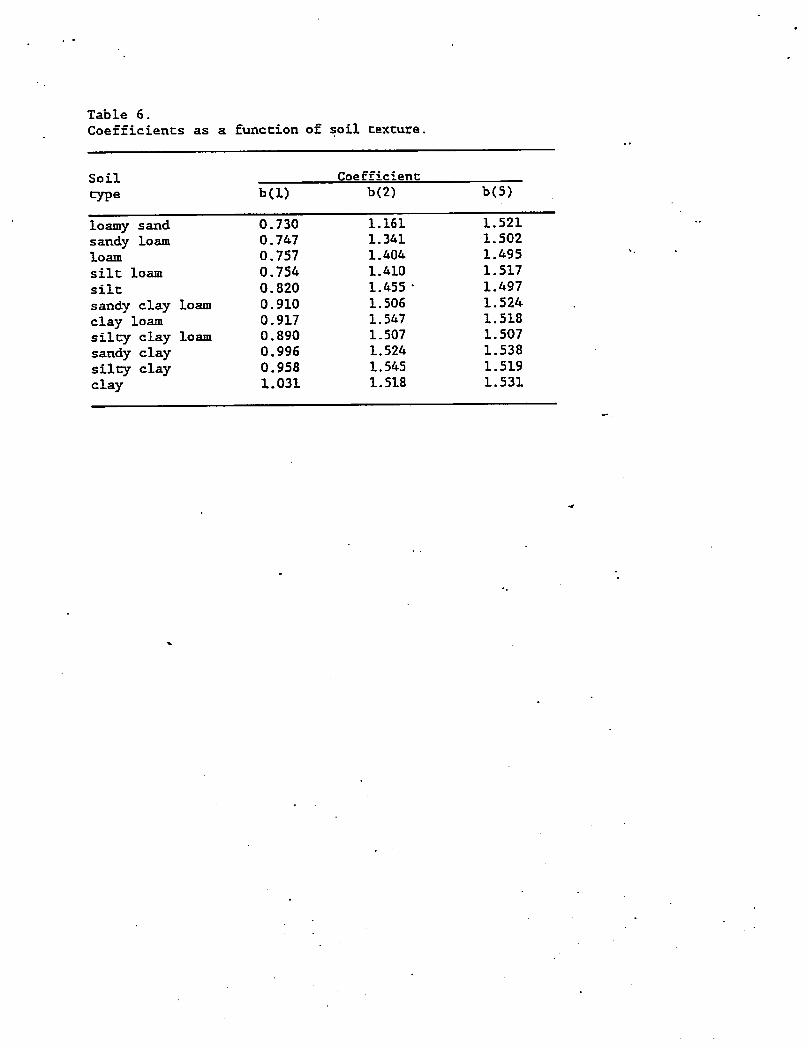
Table 6.
Coefficiencs as a funccion of soil texture.
Soil
type
loamy sand
sandy loam
loam
silt loam
silt
sandy clay loam
clay loam
silty clay loam
sandy clay
silny clay
clay
b(l)
0.730
0.747
0.757
0.754
0.820
0.910
0.917
0.890
0.996
0.958
1.031
Coefficient
b(2)
1.161
1.341
1.404
1.410
1.455 •
1.506
1.547
1.507
1.524
1.545
1.518
b(5)
1.521
1.502
1.495
1.517
1.497
1.524
1.518
1.507
1.538
1.519
1.531

Table 7.
Coefficiencs as a funccion of rainfall discribucion.
Rainfall
Discribucion
1
2
3
4
5
6
7
8
9
10
11
12
13
14
15
16
17
18
19
20
21
22
23
24
25
26
27
28
29
30
b(l)
0.639
0.669
0.634
0.555
0.502
0.230
1.186
1.127
0.995
0.951
0.827
0.488
0.889
0.820
0.488
1.081
1.199
1.040
0.925
0.856
1.378
0.831
0.9-14
0.703
0.705
0.946
1.172
0.935
1.666
0.822
Coefficienc
b(2)
1.701
1.668
1.717
1.816
1.775
4.345
1.066
1.114
1.230
1.223
1.232
1.235
1.320
1.294
1.639
1.573
1.486
1.225
1.286
1.543
1.812
1.107
0.960
1.275
1.573
1.480
1.765
1.173
1.890
1.554
b(5)
1.643
1.545
1.533
1.555
1.529
1.528
1.777
1.562
1.473
1.502
1.530
1.544
1.384
1.328
1.550
1.434
1.415
1.405
1.693
1.306
1.389
1.544
1.462
1.625
1.463
1.637
1.826
1.515
1.220
1.537

Table 8.
Values of bl, b2 and b5 as a function of soil cexcure.
Soil type Coefficient
bl b2 b5
loamy sand
sandy loam
loam
silt loam
silt
sandy clay loam
clay loam
silty clay loam
sandy clay
silty clay
clay
0.70
1.07
1.26
■
1.64
1
1
| i 51 |

Coefficietics co obcain b3 as a funccion of Dr. cp and ip.
loamy sand -0.31
sandy loam -0.48
loam -0-56
silc loam -0.53silc -0.52
sandy clay loam -0.39
clay loam , -0.40
silcy clay loam -0.37
sandy clay -0.41
silcy clay -0.40
clay -O-27
Coefficienc
;cexcure c0 cl
6.
6.
1.
3.
2.
2.
4.
4.
5.
31
73
34
17
62
80
42
25
.75
0.
0.
0.
0.
0.
0.
0.
0.
0.
0.
0.
12
12
12
13
11
09
09
09
07
.07
.05
1.
1.
1.
1.
1.
0.
0
0
0
0
0
58
45
38
,30
.13
.79
.78
.77
.79
.81
.66

Table 10.
Watershed characteristics at of storms.
Location
Watkinsville, GA
Sandy Loam, approx.
63% Sa, 21% Si. 16% Cl
Riesel, TX
70% Houston Black Clay
30% Heiden Clay
Watershed Area
(acres) (ha)
19.2
2.99
Hastings, NE
75% of area is Holdrege
silt loam & 25% is Holdrege
silty clay loam (severely
eroded)
3.77
7.77
Storm
date
3/19/70
Land use &
management.
Dormant costal
bermuda grass,
just beginning
spring growth,
excellent cover
1.21 8/12/66 100% bermudagrass pasture
2-4" high, good
cover, not
grazed
7/19/68 100% bermuda
grass pasture
10" high
1.53 7/3/59 Sorghum about 6"high and in good
condition. Weeds
beginning to
grow.
5/21/65 ■"' No tillage during
spring.
Source of Data: USDA-ARS 1963. Hydrologic data
.«*-.
Washington, DC.

Table 11.
Comparison becween kineraacic routing and approximate method.
Rainfall
03/19/70
08/12/66
07/19/68
07/03/59
05/21/65
Volume
Runoff
nm
19.9
41.8
12.5
59.7
57.9
Measured Rain
Kinematic Routine
Peak
Runoff
mm/h
7.2
40.7
21.1
163.8
79.8
Duration
Runoff
min
1,215.0
309.0
121.0
55.0
117.0
ADoroximate
Peak
Runoff
mm/h
29.3
77.7
20.9
185.6
82.6
Method
Duration
Runoff
min
2,626.7
600.0
151.7
63.5
140.0

Table 12.
Comparison becween kinematic routing and approximate method.
Rainfall
03/19/70
08/12/66
07/19/68
07/03/59
05/21/65
Volume
Runoff
33.4
54.0
12.2
59.7
56.6
Kinematic Routine
Disaggregated
Peak Duration
Runoff Runoff
mm/h min
22.2
59.0
20.3
157.1
69.5
626.0
231.0
99.0
49.0
113.0
Rain
Auoroximate
Peak
Runoff
mm/h
22.2
60.3
24.4
157.1
68.7
Method
Duration
Runoff
min
613.2
217.5
96.7
51.7
113.8