Canopy Closure Estimates with GreenOrbs: Sustainable Sensing in the Forest

§¶‡Lufeng Mo, §Yuan He, §Yunhao Liu, ¶Jizhong Zhao, †Shaojie Tang, †Xiang-Yang Li, ₣Guojun Dai

§Hong Kong University of Science and Technology ¶Xi’an Jiaotong University

‡Zhejiang Forestry University †Illinois Institute of Technology ₣Hangzhou Dianzi University

Abstract Motivated by the needs of precise forest inventory and real-time surveillance for ecosystem management, in this paper we present GreenOrbs [1], a wireless sensor network system and its application for canopy closure estimates. Both the hardware and software designs of GreenOrbs are tailored for sensing in wild environments without human supervision, including a firm weatherproof enclosure of sensor motes and a light-weight mechanism for node state monitoring and data collection. By incorporating a pre-deployment training process as well as a distributed calibration method, the estimates of canopy closure stay accurate and consistent against uncertain sensory data and dynamic environments. We have implemented a prototype system of GreenOrbs and carried out multiple rounds of deployments. The evaluation results demonstrate that GreenOrbs outperforms the conventional approaches for canopy closure estimates. Some early experiences are reported in this paper.

Categories and Subject Descriptors C.2.1 [Computer Communication Networks]: Network Architecture and Design – Distributed networks; Wireless communication; C.2.4 [Computer Communication Networks]: Distributed Systems – Distributed applications;

General Terms Measurement, Design, Experimentation.

Keywords: Wireless Sensor Network, Canopy Closure, Design, Deployment

Figure 1. Definition of canopy closure: the percentage of

ground area vertically shaded by overhead foliage

1. Introduction Human beings nowadays have an unprecedented appreciation of environmental protection and sustainable development. Ecosystem management is attracting increasing attention and gradually replacing the traditional approaches to function in various application fields [2]. Forests, “the earth’s lungs”, are among the most precious natural resources that we must preserve to regulate our climate and keep ecological balance.

Canopy closure, defined as the percentage of ground area vertically shaded by overhead foliage [3], is widely utilized as a critical indicator of the condition of a forest ecosystem. As illustrated in Figure 1, canopy closure in a forest refers to the ratio of the area shaded by the trees to the area of the entire ground. Having many significant uses for ecosystem management and disaster forecast, canopy closure estimates, however, are practically non-trivial [3, 4, 5, 6]. Most existing approaches suffer the scalability problem, due to the limited measurement capacity and high costs. The status of canopy closure largely depends on the weather (e.g. the effect of strong winds) and can be highly dynamic. The measurement procedures are also restricted by the subjectivity of the surveyor, the landform, and the undergrowth. As a result, conventional approaches can only provide inaccurate estimates.

To address this issue, we present GreenOrbs [1], a wireless sensor network (WSN) system in the forest, and its application for canopy closure estimates. In GreenOrbs, a number of commercial off-the-shelf sensor motes are

Permission to make digital or hard copies of all or part of this work for personal or classroom use is granted without fee provided that copies are not made or distributed for profit or commercial advantage and that copies bear this notice and the full citation on the first page. To copy otherwise, or republish, to post on servers or to redistribute to lists, requires prior specific permission and/or a fee. SenSys’09, November 4–6, 2009, Berkeley, CA, USA. Copyright 2009 ACM 978-1-60558-748-6...$5.00

programmed, enclosed, and deployed in the forest. With every node equipped with light, temperature, and humidity sensors, GreenOrbs supports various ecological applications. In this paper, we focus on the application for canopy closure estimates. Our contributions are summarized as follows:

1. We propose a sensor network design that enables accurate canopy closure estimates using inexpensive sensors randomly deployed in the forest;

2. We propose a technique to calibrate the light sensors and discriminate the states between light versus shade;

3. We design light-weight mechanisms for node state monitoring, which reduces communication overhead;

4. We present a detailed evaluation of GreenOrbs and compare it with conventional forestry methods. The results demonstrate the advantages of WSN techniques and their great potential benefits by introducing WSNs into the traditional forestry field.

The rest of this paper is organized as follows. Section 2 briefly introduces the background. Section 3 presents the system framework and theoretical foundation of canopy closure estimates with GreenOrbs. Section 4 elaborates on the system design. The implementation details and evaluation results are presented in Section 5. In Section 6, we briefly review previous WSN applications related to our work. Section 7 concludes the paper.

2. Background

2.1 Canopy Closure Canopy closure is a valuable forest inventory factor, which plays an important role in ecosystem management. It is actually a fundamental factor to define a forest. The current global definition of forest is an area of land that is more than 0.5 hectares with more than 10% canopy closure [7]. Canopy closure is being seen as more important recently in the sense of environmental protection. For instance, it is a key indicator of the water conservation capacity of a forest. When logging in a forest with non-uniform vegetation, the canopy closure of different areas in the forest must be considered to maintain sustainable development. In a process of urban greening, canopy closure is useful in characterizing the forest stand structure.

In ecological forestry and agriculture, canopy closure is used to estimate various indexes, such as penetration of light to the understory, absorbance of carbon dioxide, and release of oxygen, which are closely associated with photosynthesis. Continuous measurements of canopy closure reflect the growth of vegetation, and thus can be used to assist ecological planning in forestry and agriculture. Moreover, regulations for certain regional wildlife species require maintenance of certain levels of canopy cover. Real-time data of canopy closure can be used to construct precise

computational models of rain interception, so that people can better predict disasters like floods and mud-rock flows.

2.2 Canopy Closure Estimates Despite the significance of canopy closure, the usage of canopy closure is often restricted due to the lack of accurate and efficient measurement approaches. The existing approaches fall into two categories: ground measurement and aerial measurement.

With ground measurement, canopy closure is manually estimated by people or with auxiliary devices. Approaches like ocular estimate, line-intercept, and crown mapping fall into this category. Ocular estimate and line-intercept are traditional approaches using simple inexpensive instruments [3, 4]. Ocular estimate relies on an experienced surveyor conducting a long training process. Line-intercept estimates canopy closure by the percentage of shaded length on a line placed on the ground. It is efficient for estimating the profile of large crowns but often fails to capture the interspaces among the leaves inside a crown, due to the limited breadth of a line. Crown mapping [6] maps the crowns of trees with a spherical densitometer or a vertical point sampling device. Canopy closure can thus be estimated by scanning and processing the maps of crowns. Crown mapping requires careful mounting of devices, and may yield detailed estimates, while it suffers poor scalability due to the inconvenient deployment and prohibitive measuring cost. Fisheye lenses that are able to take hemispherical photographs can be used to measure the canopy of a very small area but cannot measure a vast forest.

Ground measurement approaches have two common limitations: First, various factors can often interfere in the estimated results, such as the subjectivity of the surveyor, the landform, and the undergrowth. Second, they can only measure a small portion of forest, and thus lack scalability in large-scale applications.

In order to eliminate the ground measurement limitations, aerial measurement and satellite imaging are proposed for canopy closure estimates [4, 5]. Aerial measurement estimates the canopy closure based on bird's-eye view photos of a forest. Since the photos are taken from the air at limited heights, the results are often overestimated due to the non-vertical visual angles on a large canopy. The quality of photos is highly dependant on the weather. Photos taken on a sunless day have poor contrast, while strong sunlight results in high reflection from the vegetation. Regardless, both cases lead to poor estimates of canopy closure.

Satellite imaging is the latest proposal for canopy closure estimates, but has not yet reached a mature approach. It overcomes the drawbacks of aerial measurement, but still suffers many difficulties. For example, in a satellite image, it is hard to accurately discriminate the canopy from the undergrowth.

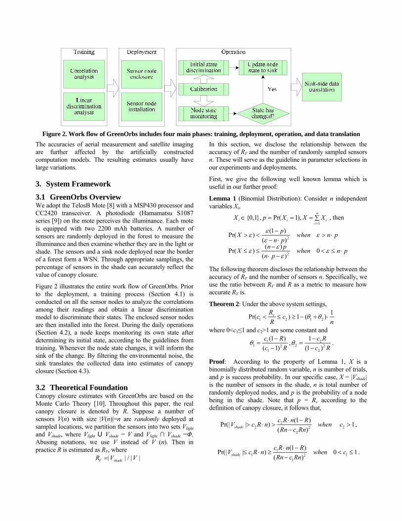
Figure 2. Work flow of GreenOrbs includes four main phases: training, deployment, operation, and data translation

The accuracies of aerial measurement and satellite imaging are further affected by the artificially constructed computation models. The resulting estimates usually have large variations.

3. System Framework

3.1 GreenOrbs Overview We adopt the TelosB Mote [8] with a MSP430 processor and CC2420 transceiver. A photodiode (Hamamatsu S1087 series [9]) on the mote perceives the illuminance. Each mote is equipped with two 2200 mAh batteries. A number of sensors are randomly deployed in the forest to measure the illuminance and then examine whether they are in the light or shade. The sensors and a sink node deployed near the border of a forest form a WSN. Through appropriate samplings, the percentage of sensors in the shade can accurately reflect the value of canopy closure.

Figure 2 illustrates the entire work flow of GreenOrbs. Prior to the deployment, a training process (Section 4.1) is conducted on all the sensor nodes to analyze the correlations among their readings and obtain a linear discrimination model to discriminate their states. The enclosed sensor nodes are then installed into the forest. During the daily operations (Section 4.2), a node keeps monitoring its own state after determining its initial state, according to the guidelines from training. Whenever the node state changes, it will inform the sink of the change. By filtering the environmental noise, the sink translates the collected data into estimates of canopy closure (Section 4.3).

3.2 Theoretical Foundation Canopy closure estimates with GreenOrbs are based on the Monte Carlo Theory [10]. Throughout this paper, the real canopy closure is denoted by R. Suppose a number of sensors V(n) with size |V(n)|=n are randomly deployed at sampled locations, we partition the sensors into two sets Vlight and Vshade, where Vlight U Vshade = V and Vlight ∩ Vshade =Φ. Abusing notations, we use V instead of V (n). Then in practice R is estimated as RV, where

| | / | |V shadeR V V=

In this section, we disclose the relationship between the accuracy of RV and the number of randomly sampled sensors n. These will serve as the guideline in parameter selections in our experiments and deployments.

First, we give the following well known lemma which is useful in our further proof:

Lemma 1 (Binomial Distribution): Consider n independent variables Xi,

1{0,1}, Pr( 1),

n

i i ii

X p X X X=

∈ = = = ∑ , then

2

2

(1 )Pr( )( )( )Pr( ) 0

( )

pX when n pn p

n pX when n pn p

εε εε

εε εε

−> < > ⋅

− ⋅−

≤ ≤ < ≤ ⋅⋅ −

The following theorem discloses the relationship between the accuracy of RV and the number of sensors n. Specifically, we use the ratio between RV and R as a metric to measure how accurate RV is.

Theorem 2: Under the above system settings,

1 2 1 21Pr( ) 1 ( )vR

c cR n

θ θ< ≤ ≥ − + ⋅

where 0<c1≤1 and c2>1 are some constant and 1

1 21

(1 )( 1)c Rc R

θ−

=−

, 22 2

2

1(1 )

c Rc R

θ−

=−

.

Proof: According to the property of Lemma 1, X is a binomially distributed random variable, n is number of trials, and p is success probability. In our specific case, X = |Vshade| is the number of sensors in the shade, n is total number of randomly deployed nodes, and p is the probability of a node being in the shade. Note that p = R, according to the definition of canopy closure, it follows that,

22 22

2

(1 )Pr(| | ) 1

( )shadec R n R

V c R n when cRn c Rn

⋅ −> ⋅ > >

−,

11 12

1

(1 )Pr(| | ) 0 1

( )shadec R n R

V c R n when cRn c Rn

⋅ −≤ ⋅ ≥ < ≤

−.

104

108

112

116

1 3 5 7 9 11 13 15 17 19 21Node ID

Perc

eive

d ill

umin

ance

(KLu

x)

Figure 3. Simultaneous readings of 21 sensors that are

placed under different illuminance in the forest

Pr( |Vshade| ≤ c1R·n ) = Pr( RV ≤ c1R ),

Pr( |Vshade| > c2R·n ) = Pr( RV > c2R ).

Then together with the property of union probability, we immediately get

1 2 1 21Pr( ) 1 ( )vR

c cR n

θ θ< ≤ ≥ − + ⋅

where 11 2

1

1( 1)

c Rc R

θ−

=−

, 22 2

2

(1 )(1 )c R

c Rθ

−=

−.

Theorem 2 represents the ideal case when every sensor can be placed into its corresponding subset (either Vlight or Vshade) correctly. Such an assumption, however, does not always hold in practice, due to the uncertainties in sensor readings and environmental dynamics (e.g. the sunlight). This is one of the major challenges we address in the following subsections. Nevertheless, Theorem 2 is useful to estimate the best attainable result with n sampled sensors.

4. Design The following key issues need to be addressed in the design of GreenOrbs. First, the sensors in GreenOrbs have diverse instrumental errors in their readings. We need to devise an effective calibration method and a model which best separates the sensors into two subsets, Vlight and Vshade. Second, considering the energy constraints on the nodes, we need an energy-efficient mechanism for state monitoring and data collection. Third, considering the varying solar altitude, a universal model is required to translate the measured percentage of sensors in the shade into an estimated canopy closure. The design of GreenOrbs mainly consists of three components: pre-deployment training, online data processing, and sink-side data translation.

4.1 Pre-deployment Training The training process yields the guidelines of online sensory data processing, namely calibration and node state discrimination.

105

110

115

120

125

1 146 291 436 581 726 871 1016 1161Time (sec)

Illum

inan

ce (K

Lux)

Node 4 Node 6 Node 8 Node 10 Node 12

Figure 4. Simultaneous readings of five sensors that are

placed under the same illuminance Accordingly, the training process is divided into two phases, correlation analysis and linear discrimination analysis.

4.1.1 Correlation Analysis Sensor readings are intrinsically error-prone. Due to the diverse instrumental errors, the raw sensor readings without calibration often result in incorrect measurements. We conduct an observational experiment to disclose the importance of calibration. We first place 21 sensors at different locations (some in the light and the others in the shade) when the environmental illuminance is 114.75Klux. Here environmental illuminance is defined as the illuminance at a location without any shade, denoting the maximum illuminance in the environment. Figure 3 shows the perceived illuminance of the sensors. The maximum difference between any two readings is 8.41KLux.

We then place the 21 sensors under exactly the same illuminance and let them sense the illuminance once every second. Note that the illuminance varies with time. The readings of five typical sensors are plotted in Figure 4. Surprisingly, the maximum difference between two sensor readings is around 6KLux. We take more rounds of the experiments and obtain similar results, indicating that the instrumental errors of sensor readings cannot be overlooked. Unless the sensor readings are appropriately calibrated, we cannot correctly estimate canopy closure.

Figure 4 indicates another fact that the instrumental errors on each individual sensor are consistent over time. Thus an intuitive guess comes into our mind: Are the readings of sensors linearly correlated with each other? Yes. To validate this answer, we take a randomly selected sensor in the above experiment as the reference and analyze the correlation between the reference and any other node.

There are a total of 21 sensors in the experiment, denoted by S0, S1, S2, ..., and S20. Let n denote the total number of readings a sensor produces. k (1≤k≤n) denotes the counter of sensor reading. Nk denotes the reading of the reference sensor S0 while Mik (i=1, 2, ..., 20) denotes the reading of Si. The

Pearson product-moment correlation coefficients [11] between S0 and Si are calculated using Equation (1).

1 1 1

2 2 2 2

1 1 1 1

( ) ( )

n n n

ik k ik kk k k

i n n n n

ik ik k kk k k k

n M N M Nr

n M M n N N

= = =

= = = =

−=

− −

∑ ∑ ∑

∑ ∑ ∑ ∑ (1)

The calculation results are shown in the second column of Table 1, which validate that the sensor readings are almost linearly correlated. Taking S0 as the reference, we can thus calibrate the readings of all the other sensors through linear transformations. Let M’ik denote the calibrated reading of Si. The linear transformation from Mik to M’ik is

ik i ik iM a M b′ = + called calibration formula, where ai and bi are the calibration coefficients for Si. To minimize the instrumental error differences between S0 and Si, ai and bi need to satisfy the following conditions. First, the expectation of M’ik equals that of Nk.

1 1

1 1( )n n

i ik i kk k

a M b Nn n= =

+ =∑ ∑ (2)

Second, ai and bi minimize the deviation of M’ik to Nk.

2

1( , ) arg min (( ) )

n

i i i ik i kk

a b a M b N=

= + −∑ (3)

Table 1: The correlation coefficients between S0 and Si and calibration coefficients of Si

Node ID (i) ri ai bi (KLux)1 0.9645 1.09 -7.76 2 0.9512 1.10 -12.93 3 0.9525 1.22 -25.62 4 0.9543 1.19 -21.98 5 0.9329 1.21 -22.83 6 0.9421 0.99 0.67 7 0.9412 1.03 -2.60 8 0.9585 0.88 14.23 9 0.9478 0.94 7.14

10 0.9666 1.07 -5.50 11 0.9635 1.12 -14.36 12 0.9637 1.01 -2.48 13 0.9555 1.18 -18.41 14 0.9555 1.11 -11.04 15 0.9780 1.04 -3.77 16 0.9498 0.91 8.68 17 0.9443 0.91 10.89 18 0.9363 1.22 -22.04 19 0.9283 0.98 2.46 20 0.9700 0.95 3.94

Average 0.9528 1.06 -6.17 Standard Deviation 0.0129 0.11 12.16

Solving Equations (2) and (3) yields the value of ai and bi as follows.

1 1 1 1 1

2 2

1 1

,( )

n n n n n

ik k ik k k i ikk k k k k

i in n

ik ikk k

M N n M N N a Ma b

nM n M

= = = = =

= =

− −= =

−

∑ ∑ ∑ ∑ ∑

∑ ∑

The last two columns of Table 1 list the calibration coefficients. Through a similar training process, we obtain the calibration formulas of all sensors to be deployed. The training results are omitted here due to the page limit. Section 5.2.1 has more details on the effectiveness of calibration.

4.1.2 Linear Discrimination Analysis A sensor cannot determine its status merely based on the perceived illuminance, even it is calibrated. For example, we observe that at one time a sensor in the shade perceived illuminance of 106.3KLux, while at another time a sensor in the light perceived illuminance of only 102KLux. The discriminating point between light and shade actually depends on the environmental illuminance. It requires both the sensor’s calibrated reading and the current environmental illuminance to get an accurate determination of the sensor’s current state. Hence, in the second phase of the training, we derive a linear discrimination model from a comprehensive training data set. Node states in the set are recorded through manual observations. The corresponding calibrated sensor readings are then collected at the sink. The reference sensor is placed under the sun to perceive the environmental illuminance. As shown in Figure 5, Point (x, y) denotes a sensor reading of y when the environmental illuminance is x. Clearly, there exists a separating boundary between Vlight and Vshade. We use the method of Least Linear Squares to derive the linear discrimination model, denoted by Y=d0+d1X. We have

20 1( )i iY d d Xφ = − −∑

110 112 114 116 118 12095

100

105

110

115

120

Environmental illuminance (KLux)

Sen

sor

read

ing

(KLu

x)

Node in the light

Node in the shade

Figure 5. The linear discrimination model

0 10

2 ( ) 0i iY d d Xdφ∂

= − − − =∂ ∑ (4)

0 11

2 ( ) 0i i iY d d X Xdφ∂

= − − − =∂ ∑ (5)

Solving Equations (4) and (5) with the training data set, we get d0=17.45, d1=0.81. Using this model, a node is able to exactly determine its current state under any environmental illuminance.

Note that as shown in Figure 5, the discrimination model produces a very small portion of false judgments when the environmental illuminance is over 115KLux. We have more discussions on this problem in Section 4.2.3.

4.2 Online Data Processing The calibration formulas and the linear discrimination model are loaded into all the nodes before deployment. Since the nodes all perceive nearly zero illuminance at night, canopy closure estimates are conducted only in the daytime. Every day sensors start operation at 8:30 a.m. and switch off at 15:30 (we explain in Section 4.3 why we set such a measurement period).

Whenever in operation, the raw readings are calibrated once they are perceived. Without special declaration, the sensor readings refer to the calibrated ones.

4.2.1 Initial State Determination The initial node states are determined based on the linear discrimination model. As soon as GreenOrbs starts in operation, nodes exchange their initial readings through gossip [12]. Every node forwards the highest reading it obtains (either its own reading or a reading from the others). The gossip process converges in O(d) time where d is the network diameter.

At the end of gossip, all the nodes possess an identical highest reading, which denotes the current environmental illuminance, denoted by X0. According to the discrimination model, the value separating Vlight and Vshade is calculated by Y0=d0+d1X0. Let yi0 denote the initial reading of Node Vi. Its initial state is determined as follows: If yi0> Y0, Vi is in the light. Otherwise, Vi is in the shade.

4.2.2 Node State Monitoring and Collection The sensing frequency of nodes in GreenOrbs is set at once per minute. Considering the degree of dynamics in the forest, such a sensing frequency is sufficient to capture all possible changes in the environment at relatively low cost.

A straightforward but inefficient method (called naive method) to monitor the node state is to let each node periodically send every reading directly to the sink. Such a method obviously incurs a huge amount of network traffic. Besides, considering the multi-hop transmission in a large WSN, concurrent data collection from all the nodes will

probably cause congestion over bandwidth-constrained wireless links, which will lead to frequent packet loss and extra retransmission cost [13].

A possible minor improvement is to execute distributed state monitoring (called gossip-based method), as we do in the initial state discrimination. Nevertheless, it requires a gossip process in the whole network to propagate the environmental illuminance in each period and still incurs considerable network traffic.

GreenOrbs realizes a light-weight mechanism for node state monitoring and data collection, which overcomes all the above drawbacks. During the whole measurement period after the initial state discrimination, a node updates its state to the sink node only when it detects a state transition from light to shade, or vice versa. We have observed that the course of a state transition lasts at least five minutes. Hence we set the periodical interval of state monitoring as five minutes. At the end of every interval, a node calculates the average of the latest five readings. Let I and I’ denote the current average and the average of the previous interval, respectively. The varying rate of readings is calculated by Vrate=(I−I’)/5. The unit is KLux/min.

Note that the varying rate of sensor readings is not directly associated with the node state. A large variation in the perceived illuminance does not necessarily imply a state transition; however, a state transition always corresponds to a large variation in the perceived illuminance on a node. The ultimate goal of our algorithm is to identify the large variations of sensor readings which indeed cause state transitions.

If the variation is caused by the swaying of leaves, the phenomenon is usually transitory so the node state stays unchanged over a relatively long period. One can filter such noises by averaging the latest sensor readings. That’s why we set the interval of state monitoring at five minutes. If the variation is caused by reflection or refraction (the change in direction of light when it irradiates or passes through the vegetation), it is really a problem that our current design cannot solve. We leave it for future work.

Great variations in environmental illuminance (i.e. the sunlight) also cause large variations in the perceived illuminance on a sensor node. For example, a floating cloud sometimes blocks out the sunshine. In this case, the perceived illuminance on the nodes greatly varies, but actually the node states stay unchanged.

The real cause of node state transitions is the change of the solar altitude. In this case, only a small portion of the nodes, namely the nodes lying near the boundary of the light and shaded areas, change their states. In this case, we would expect the Vrate of such a node to differ significantly from the average Vrate of its neighbors. This is the key idea behind our algorithm, shown in Figure 6.

Figure 6. The pseudo code of node state monitoring

Figure 6 shows the pseudo code of node state monitoring. We define two thresholds for the detection of state transitions, namely S1=6KLux/min and S2=5KLux/min. The thresholds are obtained from practical observations on node state transitions. If Vrate exceeds S1, it means the readings vary greatly and triggers the node to check whether the state has changed. Through one-hop communications, the node compares its Vrate with the AverageVrate of its neighbors. If their difference exceeds S2, it indicates that the node state has changed. Otherwise, the node state remains unchanged and probably the environmental illuminance has varied greatly.

4.2.3 Discussion Here we have a brief discussion on the effectiveness of the mechanism for node state monitoring.

9:00 a.m. 10:00 a.m. 11:00 a.m. 12:00 a.m.

Figure 7. Tree shadows with varying solar altitude

First, except for the daily starting phase, node state monitoring is based solely on local information and the data from its one-hop neighbors. Compared to the naive and gossip-based methods, it saves a large amount of energy cost.

Second, according to the observation, the daily frequency of node state transitions is 2.25 times on average, of which we have more details in Section 5.2.3. A daily measurement period includes 7ä60/5=84 intervals of state monitoring. Assuming that node transitions are uniformly distributed over the course of a day, then on average less than 3% of the nodes change their state at every interval. Hence the concurrency of data transmissions is significantly reduced and the data collection process becomes essentially asynchronous. Consequently, GreenOrbs avoids congestion over the links and further enhances the energy efficiency.

Third, as we mention in Section 4.1.2, the linear discrimination model produces a very small portion of false judgments when the environmental illuminance is over 115KLux. In GreenOrbs, however, this model is used only for initial state discrimination. Another fact is the environmental illuminance in the early morning is never over 110KLux. Therefore, those false judgments are avoided.

4.3 Sink-side Data Translation Canopy closure is calculated using the collected states of all the nodes. Recall that canopy closure is defined as the percentage of ground area “vertically” shaded by overhead foliage. Here we define the solar altitude, denoted by α (0≤α≤90±), as the angle between the direction of sunlight and the horizontal plane. Note that α is a time-varying parameter. Observed in our deployment area, α is usually less than 83± and varies with the seasons and the time of a day. Hence, the calculated percentage of sensors in the shade cannot be directly regarded as canopy closure of the forest. Calculated results at different times cannot be merged, either. We introduce a translation model, with which the measured percentage of sensors in the shade (RV) is translated into an estimate of canopy closure R. We further define Sp as the area of the crown’s vertical projection on the ground, and Sα as the area of the shade when the solar altitude is α.

pV

SR R

Sα

= × (6)

/* Node.Neighbors: the neighboring node set of Node; Node.Vrate: the varying rate of Node’s reading; Node.State: the current node state, denoted by 0 or 1; Node.Interval: the interval of state monitoring; S1, S2: the two predefined thresholds. */ void Monitoring() {

// Calculate the varying rate in the last interval. Node.Vrate=CalculateVrate(interval); // Detect a possible state transition from 0 to 1. if (Node.Vrate>S1 && Node.State==0) {

AverageVrate= GetVrate(Node.Neighbors); // Compare local Vrate with that of neighbors if (Node.Vrate−AverageVrate>S2) Node.State=1; UpdateState(); //Update the latest state to the sink

} // Detect a possible state transition from 1 to 0. else if (Node.Vrate<−S1 && Node.State==1) {

AverageVrate= GetVrate(Node.Neighbors); if (Node.Vrate−AverageVrate<−S2) Node.State=0; UpdateState();

} } // Calculate average Vrate in nodeset int GetVrate(nodeset) {

int rate=0; for (every node v in nodeset) {Request v.Vrate from node v; rate=rate+v.Vrate;} rate=rate/|nodeset|; //|nodeset| is nodeset’s cardinality return rate;

}

Figure 8. Vertical and non-vertical shades of a conic crown

Figure 9. The case of non-overlapping tree shadows

Here we need to compute Sp/Sα. As conventionally assumed in forestry [14], the crown of a tree can be modeled as a certain stereo shape, depending on the tree species. Figure 7 depicts the shadows of different trees at different times of a day, which indicates that given the tree species and the solar altitude, the tree shade is uniquely determined. Although this is an approximate model for trees, we show through the performance evaluation that estimates based on this modeling indeed have satisfactory accuracies.

Without loss of generality, we use the conic crown as an example. Figure 8 illustrates a conic crown, its vertical projection, and its shade when the solar altitude is α. We have Sp=πr2 and

22

'

'

'

2'

tan( arccos ) ,tantan(arccos )

0 arctan2

, arctan2 2

r rS rrh

hrwhenh

rS r whenh

α

α

απα

παπ ππ α

⎧= − +⎪

⎪⎪⎨ < < −⎪⎪

= − ≤ ≤⎪⎩

The tree species and the solar altitude at a given time of day are relatively static information about a forest. The sink node stores such information as offline data. By substituting the above results into Equation (6), the sink node translates the measured RV into an estimate of canopy closure R. Actually Sp/Sα is computable given the tree species and slope of the ground [15]. We assume horizontal ground here for ease of discussion.

Note that in theory, tree shadows possibly overlap each other. Here we briefly discuss this issue. Figure 9 plots two neighboring trees, where d is the distance between two

(a) (b) Figure 10. The enclosure of mote

and the deployment area neighboring trees, h is the height of the trees, h’ is the height of the crown, and r is the radius of the crown. Then the necessary condition for non-overlapping tree shadows is

( ') cot cotd r h h hα α− + − ≥ , that is 'arctan h

d rα ≥

− (7)

Note that we assume the two trees are the same shape and size, which is the case in a normal forest. We use such an assumption just to deduce the necessary condition, for example in our deployment, d≈4m, r≈1.6m, h’≈2.8m. According to (7), α≥49.3±. This condition is basically satisfied from 8:30 a.m. till 15:30 everyday in the summer. Thus we set this period as the daily measurement period. Using a similar method, we may also deduct the measurement period for any given type of forest.

5. Performance Evaluation

5.1 Implementation Enclosure. As GreenOrbs is deployed for long-term monitoring in the forest without human supervision, the sensor nodes must be firmly protected to resist possible inclement weather and physical destruction (e.g. knocks from wild animals). Otherwise, the system would suffer frequent unexpected loss of sensor nodes and thus break down in a very short space of time. We devise a firm weatherproof enclosure of the sensor node as shown in Figure 10(a). The sensor mote is enclosed by a plastic box with a transparent upper face so that the enclosure has little influence on the illuminance perceived by the sensor. The pre-deployment training process is conducted on the enclosed sensors, too.

There are holes on the side facets of the box. Recall that GreenOrbs supports many other ecological applications which require temperature and humidity data as well. Those holes let air circulate smoothly in and out, so that the temperature and humidity perceived by the sensor are same as those in the outside environment. The enclosed node is then mounted on a bracket and installed into the forest, as shown in Figure 10(a).

105

110

115

120

125

1 146 291 436 581 726 871 1016 1161Time (sec)

Illum

inan

ce (K

Lux)

Node 4 Node 6 Node 8 Node 10 Node 12

0%

20%

40%

60%

80%

100%

0 0.4 0.8 1.2 1.6 2 2.4Standard deviation (KLux)

Cum

ulat

ive

dist

ribut

ion

Before CALAfter CAL

0

0.05

0.1

0.15

0.2

0.25

0 1 2 3 4 5Times of state transitions per day

Prob

abili

ty d

ents

ity

Figure 11. Calibrated readings of 5 nodes under the same illuminance

Figure 12. Standard deviations of sensor readings before and after calibration

Figure 13. Daily frequency of node state transitions

Table 2. Confusion matrix of initial state discrimination

Real state In light In shade

In light 0.998 0.041 Result of discrimination In shade 0.002 0.959

Software. The sensor program is developed based on TinyOS 2.1. The HamamatsuS1087ParC component provides the illuminance readings, while the SensirionSht11C component provides the temperature and humidity readings. The VoltageC component is used to read data from the MCU-internal voltage sensor. The LowPowerListening interface is used to enable low power listening on duty-cycled nodes. The CollectionC component is used to support a multi-hop data collection with collection tree protocol [27].

Other than collecting the data for canopy closure estimates, we also let the nodes report their networking status, such as one-hop neighbors, link quality, and the routing path of each data packet.

Deployments. Figure 10(b) shows the satellite imagery of the deployment area on the campus of Zhejiang Forestry University, Hangzhou, China (30º15'28"N, 119º43'45"E), which is about 20,000 m2. We have carried out multiple rounds of deployments for the GreenOrbs prototype. The first deployment included 50 nodes, which commenced in July 2008, and lasted for a month. The CC2420_DEF_RFPOWER was set at 31 and the diameter of the resulting network was 6 hops. The second deployment started in early March 2009 and initially included 120 nodes. The CC2420_DEF_RFPOWER was set at 28 and the diameter of the resulting network was 10 hops.

The deployment area belongs to the north subtropical monsoon climate, where the annual average temperature is 15.3~15.9±C and the annual average precipitation is 1286~1424mm.

5.2 Effectiveness of Design This section evaluates the effectiveness of the design including calibration, initial state discrimination, and node state monitoring.

5.2.1 Calibration Figure 11 shows the calibrated readings of five typical sensors, corresponding to Figure 4. After calibration, the five sensor readings stay nearly consistent under various environmental illuminances. For further comparison, we calculate the standard deviations (STD) of all sensor readings under the same illuminance. These data are collected in the training process. Figure 12 plots the cumulative distributions of STD before and after calibration. We can see that the variations among sensor readings are significantly reduced through calibration. As a fundamental element in our design, calibration guarantees that different sensors, although having diverse instrumental errors, produce almost the same readings as long as they are under the same illuminance.

5.2.2 Accuracy of Initial State Discrimination Every morning, we organized a group of surveyors to manually annotate the initial states (i.e. in the light or in the shade) of each sensor for 20 consecutive days. Altogether 1000 node states were recorded. They are regarded as the real initial sensor states and compared with the results of initial state discrimination collected at the sink node. Table 2 is the corresponding confusion matrix. The accuracy of initial state discrimination is very high. The slightly higher false rate in judging the sensors in the shade was caused by the reflection and refraction from the surroundings. While they are an infrequent phenomenon, we will address them in our future work.

5.2.3 Node State Monitoring Figure 13 illustrates the daily frequency of node state transitions in GreenOrbs. The average frequency is 2.25 times per day, which indicates that state transitions are quite infrequent in nature. As a consequence, a large portion of the energy costs can be saved if a node only updates its state to the sink node when a state transition happens. Based on the above observation, we conduct trace-driven simulations with 100 nodes to evaluate the communication cost (measured by the average number of daily radio messages) on a node using different state monitoring methods, namely the naive method, the gossip-based method, and GreenOrbs’ light-weight method.

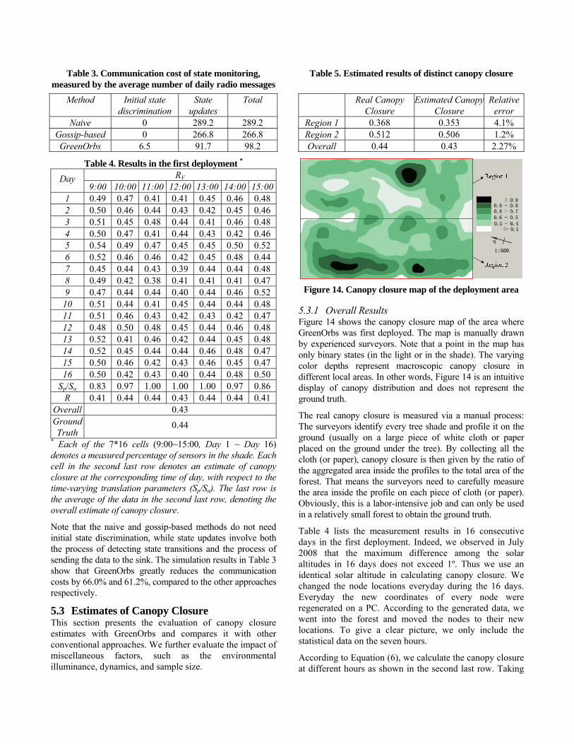
Table 3. Communication cost of state monitoring, measured by the average number of daily radio messages

Method Initial state discrimination

State updates

Total

Naive 0 289.2 289.2 Gossip-based 0 266.8 266.8 GreenOrbs 6.5 91.7 98.2

Table 4. Results in the first deployment * RV Day

9:00 10:00 11:00 12:00 13:00 14:00 15:001 0.49 0.47 0.41 0.41 0.45 0.46 0.482 0.50 0.46 0.44 0.43 0.42 0.45 0.463 0.51 0.45 0.48 0.44 0.41 0.46 0.484 0.50 0.47 0.41 0.44 0.43 0.42 0.465 0.54 0.49 0.47 0.45 0.45 0.50 0.526 0.52 0.46 0.46 0.42 0.45 0.48 0.447 0.45 0.44 0.43 0.39 0.44 0.44 0.488 0.49 0.42 0.38 0.41 0.41 0.41 0.479 0.47 0.44 0.44 0.40 0.44 0.46 0.52

10 0.51 0.44 0.41 0.45 0.44 0.44 0.4811 0.51 0.46 0.43 0.42 0.43 0.42 0.4712 0.48 0.50 0.48 0.45 0.44 0.46 0.4813 0.52 0.41 0.46 0.42 0.44 0.45 0.4814 0.52 0.45 0.44 0.44 0.46 0.48 0.4715 0.50 0.46 0.42 0.43 0.46 0.45 0.4716 0.50 0.42 0.43 0.40 0.44 0.48 0.50

Sp/Sα 0.83 0.97 1.00 1.00 1.00 0.97 0.86R 0.41 0.44 0.44 0.43 0.44 0.44 0.41

Overall 0.43 Ground Truth

0.44 * Each of the 7*16 cells (9:00~15:00, Day 1 ~ Day 16) denotes a measured percentage of sensors in the shade. Each cell in the second last row denotes an estimate of canopy closure at the corresponding time of day, with respect to the time-varying translation parameters (Sp/Sα). The last row is the average of the data in the second last row, denoting the overall estimate of canopy closure.

Note that the naive and gossip-based methods do not need initial state discrimination, while state updates involve both the process of detecting state transitions and the process of sending the data to the sink. The simulation results in Table 3 show that GreenOrbs greatly reduces the communication costs by 66.0% and 61.2%, compared to the other approaches respectively.

5.3 Estimates of Canopy Closure This section presents the evaluation of canopy closure estimates with GreenOrbs and compares it with other conventional approaches. We further evaluate the impact of miscellaneous factors, such as the environmental illuminance, dynamics, and sample size.

Table 5. Estimated results of distinct canopy closure

Real Canopy Closure

Estimated Canopy Closure

Relative error

Region 1 0.368 0.353 4.1% Region 2 0.512 0.506 1.2% Overall 0.44 0.43 2.27%

Figure 14. Canopy closure map of the deployment area

5.3.1 Overall Results Figure 14 shows the canopy closure map of the area where GreenOrbs was first deployed. The map is manually drawn by experienced surveyors. Note that a point in the map has only binary states (in the light or in the shade). The varying color depths represent macroscopic canopy closure in different local areas. In other words, Figure 14 is an intuitive display of canopy distribution and does not represent the ground truth.

The real canopy closure is measured via a manual process: The surveyors identify every tree shade and profile it on the ground (usually on a large piece of white cloth or paper placed on the ground under the tree). By collecting all the cloth (or paper), canopy closure is then given by the ratio of the aggregated area inside the profiles to the total area of the forest. That means the surveyors need to carefully measure the area inside the profile on each piece of cloth (or paper). Obviously, this is a labor-intensive job and can only be used in a relatively small forest to obtain the ground truth.

Table 4 lists the measurement results in 16 consecutive days in the first deployment. Indeed, we observed in July 2008 that the maximum difference among the solar altitudes in 16 days does not exceed 1º. Thus we use an identical solar altitude in calculating canopy closure. We changed the node locations everyday during the 16 days. Everyday the new coordinates of every node were regenerated on a PC. According to the generated data, we went into the forest and moved the nodes to their new locations. To give a clear picture, we only include the statistical data on the seven hours.

According to Equation (6), we calculate the canopy closure at different hours as shown in the second last row. Taking

0.390

0.389

0.428

0.426

0.429

0.440

0.10 0.20 0.30 0.40 0.50 0.60

0

2

4

6

8

1 3 5 7 9 11 13 15Day

Illum

inat

ion

inde

x

0%

1%

2%

3%

Rel

ativ

e er

rors

of e

stim

ates

Illumination indexRelative errors of estimates

0

0.2

0.4

0.6

0.8

1

0.00% 1.00% 2.00% 3.00% 4.00% 5.00% 6.00% 7.00%Relative errors of estimates

Cum

ulat

ive

dist

ribut

ion

N=50N=100N=200N=400N=800

Figure 15. Estimated results with different approaches

Figure 16. Impact of environmental illuminance

Figure 17. Estimation accuracy with different sample sizes

the average, we get the overall estimated canopy closure as 0.43. The real canopy closure is 0.44. Compared to the real canopy closure, the relative error of GreenOrbs’ estimate is only 2.27%.

Note that the estimated results at 10:00, 11:00, 12:00, 13:00, and 14:00 are very accurate, while the estimates at 9:00 and 15:00 are a bit smaller. This is due to the partially overlapping shadows of the trees. Recall the necessary condition in Section 4.3, the tree shadows do not overlap when α≥49.3±. On the other hand, α=45± at 9:00 and 15:00, which leads to slightly overlapping tree shadows in some places. Thus Sα is overestimated and the estimated results become slightly smaller.

In order to examine the accuracy of GreenOrbs’ estimates, we further divide the entire deployment area into two sub-regions as shown in Figure 14, which apparently have different canopy closures. Table 5 compares the real and estimated canopy closures with GreenOrbs. When the canopy closure gets larger, the estimation accuracy becomes slightly higher too. This is consistent with our theoretical conclusion in Section 3.2.

5.3.2 Comparison Now we compare GreenOrbs with the conventional approaches for canopy closure estimates, such as ocular estimates, line-intercept, crown mapping, and satellite imaging. The ocular estimates are carried out by experienced surveyors 10 times. The line-intercept estimates are conducted three times, by placing a line along three different directions on the forest ground. The crown mapping estimate is conduct only once, because of the prohibitive measuring cost. Estimates with digital photography are conducted nine times based on nine different sample areas in the forest. The result of GreenOrbs corresponds to the overall estimate in Table 4.

Figure 15 compares the estimated results of all the above methods to the real canopy closure. The maximum errors of each method are marked as well, if applicable. We can see that GreenOrbs outperforms all the other methods with the best accuracy and the highest consistency. Clearly, crown

mapping has comparable accuracy with GreenOrbs, while it is not scalable in large-scale measurement due to the prohibitive cost.

5.3.3 Impact of Environmental Factors In this subsection, we evaluate the impact of environmental illuminance on the estimation accuracy. For this purpose, we define the illumination index of a day as shown in Table 6. If there are two or more states of weather in a day, the illumination index is calculated as the average of multiple indexes. For example, a cloudy to showery day has an illumination index of 3.

Figure 16 plots the daily estimated results and illumination indexes of 16 consecutive days. Interestingly, we see strong correlation between them. Specifically, GreenOrbs achieves more accurate estimates on sunny days, because the nodes in the shade differ more distinctly from the nodes in the light in stronger sunlight. When a node state transition happens, the perceived illuminance on the sensor also presents a larger varying rate. Consequently, the accuracy of GreenOrbs’ state monitoring algorithm is higher, too.

5.3.4 Impact of Sample Size Now we perform offline analysis based on the collected data to evaluate the impact of sample size on the estimation accuracy. Everyday during the first GreenOrbs deployment, we randomly assigned the node locations, the number of sampled locations (denoted by N) represented by the collected data set is much larger than the system size (n).

For each sample size, we conduct 105 times the random samplings from the whole collected data set and therefore obtain 105 estimates of canopy closure. Figure 17 shows the

Table 6. Definition of illumination index of a day

Weather Illumination index Fine 1

Cloudy 2 Showery 4

Rainy 8

20 40 60 80 100 1200

0.2

0.4

0.6

0.8

1

Distance (m)

LQI

Temperature: 6~14 °C Humidity: 90%Temperature: 11~26 °C Humidity: 50%Temperature: 6~12 °C Humidity: 50%

Figure 18. LQI under varying temperature and humidity

cumulative distribution of relative errors. The results demonstrate that GreenOrbs is able to provide satisfactory estimates, even when we use only 50 samples. The average relative error is 4.69% when N=50. Meanwhile, the estimation accuracy increases when the sample size is increased. However, the benefit from involving more samples is slight, especially when the sample size exceeds 200. When N=200 and N=800, the average relative errors are 3.12% and 2.97%, respectively.

Here we give a brief summary of the evaluation results. We have validated the design of GreenOrbs. Specifically, calibration eliminates the diverse instrumental errors among different sensors and the results of the initial state monitoring are very accurate. The light-weight mechanism for state monitoring saves the communication cost. The results clearly demonstrate that GreenOrbs outperforms all the conventional methods. It produces accurate and consistent estimates of canopy closure with various parameter settings, such as different canopy closure, varying solar altitude, different environmental illuminance, and different sample sizes. The impacts of the above factors are also carefully assessed.

5.4 Observations on GreenOrbs 5.4.1 Power Consumption We have measured the current on each sensor node. The current on a GreenOrbs node is 19.0 mA when the radio power is on, and varies from 13.1~16.2 uA when the radio power is off. In the first deployment of GreenOrbs, we did not adopt any duty cycling mechanism and the batteries ran out in about 100 hours, which was insufficient to support continuous environmental surveillance for months.

In order to prolong the battery lifetime, since the second deployment of GreenOrbs, we have incorporated the built-in software interface of low power listening in TinyOS 2.1 and let the nodes work at 5% duty cycles. Thus we can roughly estimate the daily power consumption on a GreenOrbs node as 23.5 mAh. Given the battery capacity (2200 mAh), the

node lifetime should be more than 60 days. This is a conservative estimate, considering that some batteries stop working before it depletes all the power.

The system lifetime can be further prolonged by using more powerful batteries or a solar panel charging solution [16]. Indeed, we are planning to do so in the near future.

5.4.2 Environment-sensitive Link Quality Since GreenOrbs is deployed in the forest, we are interested to observe the interactions between the system and the environmental factors, such as temperature and humidity. Although researchers have discovered the impact of environmental factors on the wireless link quality, the relationship is a long way from being clearly disclosed.

Here we use the Link Quality Indicator (LQI) [8] as a metric to measure the wireless link quality, which is then measured under varying temperatures and humidity during the operations of GreenOrbs. Figure 18 plots LQI between two nodes as a function of node distance in three different scenarios, where the temperature and humidity differ from one another.

We can see that both temperature and humidity have certain impacts on LQI, while neither impact is remarkable. The observational results show that LQI slightly decreases when the humidity goes down, and slightly decreases when the temperate goes up. The impact becomes more apparent when the node distance is longer.

5.4.3 Environment-sensitive Network Topology Due to the broadcast nature of wireless communications in WSNs, a packet can be sent from a source node to the sink node via different intermediate relaying nodes. On the other hand, based on the observations in Section 5.4.2, the link qualities among nodes are indeed affected by the environmental factors. Thus we guess the network topology in GreenOrbs is also environment-sensitive.

By letting all the nodes along a data collection path to the sink node (including the source node) piggy-back their node IDs on the packets, we collect a number of snapshots of network topologies at different times, via which data are transmitted.

Figure 19 shows two snapshots of the network topologies in GreenOrbs, which correspond to different environmental conditions. It is interesting to see two distinctive network topologies as well. Moreover, we quantify the topological dynamics as follows. For a node, the parent node switch for data collection is regarded as a change of topology. We then measure the ratio of topological changes to the total number of collected packets. The average ratio is 5.4% and the standard deviation is 6.0%, which indicates that the network topologies exhibit certain dynamics along with the varying environmental factors.

(a) Temperature: 31±C

Humidity: 65% (b) Temperature: 23±C

Humidity: 92% Figure 19. Two snapshots of the network topologies: each line represents a link between two sensor nodes

Our observational results may be employed as a guide for practical WSN deployments as well as networking designs. Without regard to other factors (e.g. obstacles inside the deployment area), it generally requires lower density of nodes in a cool moist environment than in a warm dry environment. Further, if a WSN has the ability to sense temperature and humidity (such as GreenOrbs), it is feasible it can predicate the changes in routing-related factors (e.g. LQI) and network topologies. Thus intelligent and more efficient protocols for routing and topology control can be designed, which are proactive in dynamic environments.

6. Related Work He et al. in [17] present the design and implementation of multi-dimensional power management strategies in VigilNet, a surveillance application using power-constrained sensor devices. In order to increase the system lifetime, they propose a novel tripwire service with an effective sentry and duty cycle scheduling in the system.

An early study of WSNs for habitat monitoring is reported by Mainwaring et al. in [18]. They present an instance of WSN for monitoring seabird nesting environments and behaviors. Several issues are investigated, such as the hardware design of the sensors, the design of the network architecture, and capabilities for remote data access and management.

There are many other WSN applications for environmental surveillance. We summarize a few typical examples as follow. Tolle et al. [19] have developed a WSN to monitor a redwood tree by installing nodes throughout the tree. The sensory data are logged every 5 minutes and transmitted via a GPRS modem to an external computer. Selavo et al. [20] create a WSN for measuring light intensity, using a hierarchical architecture which includes distributed reliable storage, delay-tolerant networking, and deployment time validation techniques. They performed a field experiment over one day with seven nodes and installed 19 sensor nodes

in another experiment. Werner-Allen et al. [21] present the science-centric evaluation of a WSN deployment at an active volcano in Ecuador. Each of the 16 nodes continuously sample seismic and acoustic data during a 19-day test. Barrenetxea et al. [22] share their experience in the SensorScope system with its multiple campaigns in various environments. Xu et al. [23] present the design of a WSN system for structural data acquisition. Similarly, Li et al. present the design of an underground structure monitoring system using WSNs [24] and in particular address the issue of safety assurance in underground coal mines.

Compared to the previous work, the main novelty of GreenOrbs lies in a new WSN application, which is not just generic habitat monitoring, but quantitative measurement of canopy closure. Moreover, we present a thorough evaluation of GreenOrbs and compare it with the conventional forestry methods. The results demonstrate the advantage of WSN techniques and the great potential benefit of introducing WSN to traditional forestry.

7. Conclusion and Future Work We present GreenOrbs, a WSN system in the forest, and its application for canopy closure estimates. Canopy closure estimates are a fundamental task in ecosystem management, but have not been well addressed thus far. In every respect, the design of GreenOrbs is tailored to WSN deployments in wild environments. We have examined the effectiveness of this design and evaluated the performance through comprehensive experiments.

The current design of GreenOrbs is admittedly in its early stages. When adding a node to the system, the new node has to undergo the pre-deployment training process before being added into the network. Also, the failure of the reference node will cause problems during calibration. We will address these issues and seek more efficient calibration methods in future work. We also plan to observe the impacts of other environmental factors (e.g. the wind and tree species) on GreenOrbs’ performance. The current design will then be extended to measuring an irregular forest with a variety of tree species. We are now expanding the GreenOrbs system to a 1200 node scale in Tianmu Mountain. More details are reported in the project website [1].

8. Acknowledgements The authors would like to thank the shepherd, Matt Welsh, for his constructive feedback and valuable input. Thanks also to anonymous reviewers for reading this paper and giving valuable comments.

This work is supported in part by the NSFC/RGC Joint Research Scheme N_HKUST 602/08, the National Basic Research Program of China (973 Program) under grants No. 2006CB303000 and No. 2010CB328100, the National High Technology Research and Development Program of China

(863 Program) under grant No. 2007AA01Z180, NSFC under grants No. 60773042, No. 60828003, and No.60803126, the NSF Zhejiang under Grant No.Z1080979, the Hong Kong RGC under Grant HKBU 2104/06E, CERG under Grant PolyU-5232/07E, and NSF CNS-0832120.

9. References [1] GreenOrbs, http://www.greenorbs.org/ [2] R. E. Grumbine, "What Is Ecosystem Management?"

Conservation Biology, vol. 8, pp. 27-38, 1994. [3] F. L. Bunnell and D. J. Vales., "Comparison of Methods

for Estimating Forest Overstory Cover: Differences among Techniques," Can. J. Forest Res., vol. 20, 1990.

[4] A. C. S. Fiala, S. L. Garman, and A. N. Gray, "Comparison of Five Canopy Cover Estimation Techniques in the Western Oregon Cascades," Forest Ecol. Manag., vol. 232, pp. 188-197, 2006.

[5] L. Korhonen, K. T. Korhonen, M. Rautiainen, and P. Stenberg., "Estimation of Forest Canopy Cover: A Comparison of Field Measurement Techniques," Silva Fenn., vol. 40, pp. 577-588, 2006.

[6] S. R. Englund, J. J. O'Brian, and D. B. Clark, "Evaluation of Digital and Film Hemispherical Photography and Spherical Densiometry for Measuring Forest Light Environments," Can. J. Forest Res., vol. 30, pp. 1999-2005, 2000.

[7] FRA 2000 On Definitions of Forest and Forest Change, http://www.fao.org/docrep/006/ad665e/ad665e00.htm

[8] J. Polastre, R. Szewczyk, and D. Culler, "Telos: Enabling Ultra-Low Power Wireless Research," in Proceedings of IEEE IPSN, 2006.

[9] Si photodiode S1087/S1133 Series, http://sales.hamamatsu.com/assets/pdf/parts_S/S1087_etc.pdf

[10] "Monte Carlo theory and practice," Rep. Prog. Phys., vol. 43, pp. 1145-1189, 1980.

[11] D. Moore, Basic Practice of Statistics, 4 ed: WH Freeman Company, 2006.

[12] V. Ravelomanana, "Optimal Initialization and Gossiping Algorithms for Random Radio Networks," IEEE Transactions on Parallel and Distributed Systems, pp. 17-28, 2007.

[13] J. Kang, Y. Zhang, and B. Nath, "TARA: Topology-Aware Resource Adaptation to Alleviate Congestion in Sensor Networks," IEEE Transactions on Parallel and Distributed Systems, pp. 919-931, 2007.

[14] A. Cescatti, "Modeling the radiative transfer in discontinuous canopies of asymmetric crowns. II. Model testing and application in a Norway spruce stand," Ecological Modeling, vol. 101, pp. 275-284, 1997.

[15] L. Zhang, H. Yu, H. Yang, and Z. Zhang, "Theoretical Research on a Model for Predicting the Shadow Boundary of an Individual Conical Crown on a Slope," ACTA ECOLOGICA SINICA, vol. 26, pp. 3317-3323, 2006.

[16] P. Dutta, J. Hui, J. Jeong, S. Kim, C. Sharp, J. Taneja, G. Tolle, K. Whitehouse, and D. Culler, "Trio: Enabling Sustainable and Scalable Outdoor Wireless Sensor Network Deployments," in Proceedings of IEEE IPSN, Nashville, TN, USA, 2006.

[17] T. He, P. Vicaire, T. Yan, Q. Cao, G. Zhou, L. Gu, L. Luo, R. Stoleru, J. A. Stankovic, and T. F. Abdelzaher, "Achieving Long-Term Surveillance in VigilNet," in Proceedings of IEEE INFOCOM, 2006.

[18] A. Mainwaring, J. Polastre, R. Szewczyk, D. Culler, and J. Anderson, "Wireless Sensor Networks for Habitat Monitoring," in Proceedings of ACM International Workshop on Wireless Sensor Networks and Applications, 2002.

[19] G. Tolle, J. Polastre, R. Szewczyk, N. Turner, K. Tu, S. Burgess, D. Gay, P. Buonadonna, W. Hong, T. Dawson, and D. Culler, "A Macroscope in the Redwoods," in Proceedings of ACM SenSys, 2005.

[20] L. Selavo, A. Wood, Q. Cao, T. Sookoor, H. Liu, A. Srinivasan, Y. Wu, W. Kang, J. Stankovic, D. Young, and J. Porter, "LUSTER: Wireless Sensor Network for Environmental Research," in Proceedings of ACM Sensys, Sydney, Australia, 2007.

[21] G. WernerAllen, K. Lorincz, J. Johnson, J. Lees, and M. Welsh, "Fidelity and Yield in a Volcano Monitoring Sensor Network," in Proceedings of OSDI, 2006.

[22] G. Barrenetxea, F. Ingelrest, G. Schaefer, and M. Vetterli, "The Hitchhiker's Guide to Successful Wireless Sensor Network Deployments," in Proceedings of ACM SenSys, 2008.

[23] N. Xu, S. Rangwala, K. K. Chintalapudi, D. Ganesan, A. Broad, R. Govindan, and D. Estrin, "A wireless sensor network For structural monitoring," in Proceedings of ACM SenSys, 2004.

[24] M. Li and Y. Liu, "Underground Structure Monitoring with Wireless Sensor Networks," in Proceedings of IEEE IPSN, 2007.