Copula-Based Regression Estimation and Inference

Hohsuk Noh∗ Anouar El Ghouch † Taoufik Bouezmarni‡

April 4, 2012

Abstract

In this paper we investigate a new approach of estimating a regression function based on copulas.

The main idea behind this approach is to write the regression function in terms of a copula and

marginal distributions. Once the copula and the marginal distributions are estimated we use the

plug-in method to construct the new estimator. Because various methods are available in the

literature for estimating both a copula and a distribution, this idea provides a rich and flexible

alternative to many existing regression estimators. We provide some asymptotic results related to

this copula-based regression modeling when the copula is estimated via profile likelihood and the

marginals are estimated nonparametrically. We also study the finite sample performance of the

estimator and illustrate its usefulness by analyzing data from air pollution studies.

1 Introduction

Let X = (X1, . . . , Xd)⊤ be a random vector of dimension d ≥ 1 and Y be a random variable with

cumulative distribution function (c.d.f.) F0 and density function f0. Y is our response variable and

X is our set of covariates. We denote by Fj the c.d.f. of Xj and we denote by fj its corresponding

density. For a given x = (x1, . . . , xd)⊤ we will use F (x) as a shortcut for (F1(x1), . . . , Fd(xd)). From

the inspiring work of Sklar (1959), the c.d.f. of (Y,X⊤)⊤ evaluated at (y,x⊤) can be expressed as

∗Universite catholique de Louvain. H. Noh acknowledges financial support from IAP research network P6/03 of the

Belgian Government (Belgian Science Policy).†Universite catholique de Louvain. A. El Ghouch acknowledges financial support from IAP research network P6/03

of the Belgian Government (Belgian Science Policy), and from the contract ‘Projet d’Actions de Recherche Concertees’

(ARC) 11/16-039 of the ‘Communaute francaise de Belgique’, granted by the ‘Academie universitaire Louvain’.‡Departement de Mathematiques , Universite de Sherbrooke, Sherbrooke, Quebec, Canada J1K 2R1. E-mail:

taoufik.bouezmarni@usherbrooke.ca. TEL: +1-819 821 8000 #62035; FAX: +1-819 821-7189.

1

C(F0(y),F (x)), where C is the copula distribution of (Y,X⊤)⊤, that is, the function from [0, 1]d+1 to

[0, 1] defined by C(u0, u1, . . . , ud) = P (F0(Y ) ≤ u0, F1(X1) ≤ u1, . . . , Fd(Xd) ≤ ud). This is nothing

but a joint distribution function with margins that are uniform over the unit interval [0, 1]. Using

copulas allows a complete separation of dependence modeling from the marginal distributions and by

specifying a copula we summarize all the dependencies between margins, see Nelsen (2006) for more

about this subject. From the definition of copula function, the conditional density of Y given X⊤ is

given by f0(y)c(F0(y),F (x))

cX(F (x)), where c(u0,u) ≡ c(u0, u1, . . . , ud) =

∂d+1C(u0, u1, . . . , ud)

∂u0∂u1 . . . ∂udis the copula

density corresponding to C and cX(u) ≡ cX(u1, . . . , ud) =∂dC(1, u1, . . . , ud)

∂u1 . . . ∂udis the copula density of

X. Obviously, the conditional mean, m(x), of Y given X = x can be written as

m(x) = E(Y w(F0(Y ),F (x))) =e(F (x))

cX(F (x)), (1)

where w(u0,u) = c(u0,u)/cX(u) and

e(u) = E(Y c(F0(Y ),u)) =

∫ 1

0F−10 (u0)c(u0,u)du0. (2)

The equality (1) shows that, given the marginals, one can obtain the mean regression function relating

Y to X directly from the copula density, or equivalently the copula distribution of (Y,X⊤)⊤. It also

implies that the conditional mean is “just” a weighted mean with weights induced by the unknown

“conditional” copula function w defined above. This relation is not new and has been already applied

in Sungur (2005), Leong and Valdez (2005) and Crane and Van Der Hoek (2008) to compute the mean

regression function corresponding to several well known copula families (Gaussian, t, Farlie-Gumbel-

Morgenstern (FGM), Iterated FGM, Archimedean, etc.) with single (d = 1) and multiple covariate(s).

To illustrate the idea, we briefly cite two examples :

• If the copula density of (Y,X1) belongs to the FGM family with a parameter θ, i.e. c(u0, u1) =

1 + θ(1− 2u0)(1− 2u1), then we have

m(x1) = E(Y ) + θ(2F1(x1)− 1)

∫

F0(y)(1− F0(y))dy. (3)

A similar formula holds for the multiple covariate case; see Leong and Valdez (2005) .

• Let ρ = (corr(Y,X1), . . . , corr(Y,Xd))⊤ and ΣX denote the correlation matrix of X. If the

copula of (Y,X⊤)⊤ is Gaussian, then we have

m(x) = E[F−10 (Φ(u⊤Σ−1

Xρ+

√

1− ρ⊤Σ−1X

ρZ))], (4)

2

where u = (Φ−1(F1(x1)), . . . ,Φ−1(Fd(xd)))

⊤, Z ∼ N (0, 1) and Φ is the standard normal cumu-

lative distribution function.

Note that in the single covariate case we have, cX(u) ≡ cX1(u1) = 1 for all u1 ∈ [0, 1]. In such a case

the weight function w coincides with the copula density c and (1) reduces to m(x1) = e(F1(x1)) =

E(Y c(F0(Y ), F1(x1))). Also, if the covariates are mutually independent then cX(u) = 1 and m(x)

coincides with e(F (x)). In other words, e(F (x)), the numerator of m(x) in (1), is the mean regression

function of Y given X assuming independence between the covariates or, equivalently, assuming that

the conditional density of Y |X is f0(y)c(F0(y),F (x)). Thus, in term of copulas, the mean regression

function is the ratio of a numerator that only captures the mean dependence between Y and X and

a denominator that captures the dependence within X.

The equality (1) can also be used as an estimating equation. In fact, if w, F0 and Fj are any given

estimators for w, F0 and Fj , respectively, then m can obviously be estimated by

m(x) =

∫ ∞

−∞yw(F0(y), F (x))dF0(y), (5)

where F (x) = (F1(x1), . . . , Fd(xd))⊤. To the best of our knowledge, such an approach has never been

proposed or investigated in the literature in neither single nor multiple covariate case. To estimate

w, one needs an estimator for the copula densities c and cX . The copula density cX can be obtained

form c by integration. In fact,

cX(u) =

∫ ∞

−∞f0(y)c(F0(y),u))dy =

∫ 1

0c(u0,u)du0 (6)

Therefore, given an estimator c for c, one can easily estimate cX using the plug-in method and then

estimate m by (5).

Since, in the literature, there are many different methods available for estimating a copula and a

c.d.f., m(x) defines a new large class of interesting estimators. Depending on the method to estimate

the components in (5), m(x) can be a nonparametric or a semiparametric or a fully parametric

estimator. For example, using a nonparametric estimators for c, F0 and Fj , j = 1 . . . , d, leads to

a fully nonparametric estimator. Nonparametric methods for estimating c include kernel smoothing

estimators (see for example Gijbels and Mielniczuk (1990), Charpentier et al. (2006) and Chen and

Huang (2007) ) and Bernstein estimator (see Bouezmarni et al. (2010)) to cite only two examples.

In spite of the great flexibility of nonparametric methods, they are typically affected by the curse of

dimensionality and they come with the difficult problem of selecting a good smoothing parameter. On

3

the other hand imposing a parametric structure on both the copula and marginal distributions can lead

to severely biased and inconsistent (fully parametric) estimator in case of misspecification. For this

reason and in order to avoid, as much as possible, these problems, we consider here a semiparametric

approach where the copula is modeled parametrically but the marginal distributions are modeled

nonparametrically. As it is shown in the next sections, the proposed method has many interesting

properties both from theoretical and practical point of view. Especially, the asymptotic properties

are easy to obtain, the numerical calculations can be done directly using existing packages and, unlike

many semiparametric methods, no iteration procedure is needed to guarantee the consistency. Also,

the asymptotic variance can be estimated without any extra complications.

The plan of the paper is as follows. Section 2 presents the general theoretical framework of the

method with the necessary notations and assumptions. In Section 3, we establish the asymptotic

representation of the proposed estimator in the univariate and multivariate case. From this repre-

sentation we establish the asymptotic distribution and the asymptotic variance of the estimator. In

Section 4, we study theoretical properties of the estimator under misspecification. In Section 5 we

provide a simulation exercise to evaluate the performance and investigate the finite sample properties

(under correct and misspecified copula model). Finally, we analyze data from air pollution studies to

illustrate the usefulness of the proposed estimator in Section 6. Proofs appear in the Appendix.

2 Theoretical Background

Let (Yi,X⊤i ), i = 1, . . . , n, be an independent and identically distributed (i.i.d.) sample of n observa-

tions generated from the distribution of (Y,X⊤). For each i, let Xi = (Xi,1, . . . , Xi,d)⊤ and let f0 (F0)

and fj (Fj) be the density (c.d.f.) of Yi and Xi,j , respectively. Clearly, the shape and the performance

of our estimator m in (5) will heavily depend on the methods of estimation for c, F0 and Fj . In this

work, F0 is estimated empirically by

F0(y) =1

n

n∑

i=1

I(Yi ≤ y).

Estimating the other c.d.f.’s Fj , j = 1, . . . , d, can also be done empirically via Fj . However, this results

in a nonsmooth estimate m(x) as it is illustrated in Figure 1, where we show the resulting estimator

using F1 in the univariate linear case. To get a more visually attractive regression curve, one should

smooth the empirical c.d.f. The simple way to do that is to use a kernel smoothing method. Let k(·)be a function which is a symmetric probability density function and h ≡ hn → 0 be a bandwidth

4

parameter. Then, a kernel smoothing estimator of Fj is given by

Fj(x) =1

n

n∑

i=1

K

(

x−Xi,j

h

)

,

where K(x) =∫ x−∞ k(t)dt. The estimator Fj is asymptotically equivalent to Fj , in the sense that, if

nh4 → 0, then Fj satisfies the following assumption.

Assumption A:

Fj(x) = n−1n∑

i=1

I(Xi,j ≤ x) + op(n−1/2) for j = 1, . . . , d.

Evidently, this assumption also holds for the empirical c.d.f. as well as for the rescaled empirical c.d.f.

(n/(n+ 1))Fj .

Before delving into the asymptotic analysis of m, we run a small simulation study to examine

the effect of the methods of estimating F1 on the regression fit. We generate (Y,X1) using FGM

copula according to the data generating procedure DGP.S.b described in Section 5. Table 1 shows

the empirical integrated mean squared errors (IMSE), see (11) below, together with the empirical

integrated biases (IBIAS) and empirical integrated variances (IVAR) of m based on 1000 replications.

We compare the performance of m using the three estimators of F1: F1 the empirical c.d.f., Fopt the

kernel smoothing estimates with the mean square optimal bandwidth, i.e.

hopt(x1) =

[

2f1(x1)∫

tk(t)K(t)dt

(∫

t2k(t)dt)2{f ′1(x1)}2

]1/3

n−1/3,

and Fcv the kernel smoothing estimates with a bandwidth chosen via the cross-validation method.

Compared to the empirical distribution estimate, we see that the kernel smoothing estimate gives

better results if the optimal bandwidth is used. When the bandwidth is chosen by the data, its

performance is similar to the non-smooth estimator F1. This latter leads to a less biased regres-

sion estimator but with slightly large variance. Figure 1, which shows the boxplots of the empirical

integrated squared errors (ISE), also supports this observation. In this simulation the copula was

estimated using maximum pseudo-likelihood method as described below.

5

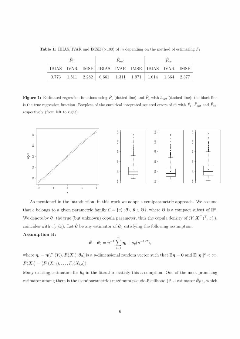
Table 1: IBIAS, IVAR and IMSE (×100) of m depending on the method of estimating F1

F1 Fopt Fcv

IBIAS IVAR IMSE IBIAS IVAR IMSE IBIAS IVAR IMSE

0.773 1.511 2.282 0.661 1.311 1.971 1.014 1.364 2.377

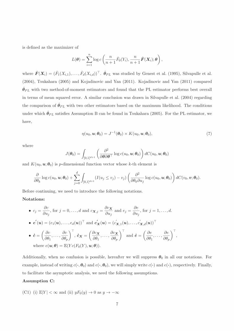
Figure 1: Estimated regression functions using F1 (dotted line) and F1 with hopt (dashed line); the black line

is the true regression function. Boxplots of the empirical integrated squared errors of m with F1, Fopt and Fcv,

respectively (from left to right).

−2 −1 0 1 2

0.0

0.5

1.0

1.5

2.0

x

m(x

)

0.00

0.02

0.04

0.06

0.08

0.10

0.00

0.02

0.04

0.06

0.08

0.10

0.00

0.02

0.04

0.06

0.08

0.10

As mentioned in the introduction, in this work we adopt a semiparametric approach. We assume

that c belongs to a given parametric family C = {c(.;θ), θ ∈ Θ}, where Θ is a compact subset of Rp.

We denote by θ0 the true (but unknown) copula parameter, thus the copula density of (Y,X⊤)⊤, c(.),

coincides with c(.; θ0). Let θ be any estimator of θ0 satisfying the following assumption.

Assumption B:

θ − θ0 = n−1n∑

i=1

ηi + op(n−1/2),

where ηi = η(F0(Yi),F (Xi);θ0) is a p-dimensional random vector such that Eη = 0 and E||η||2 < ∞.

F (Xi) = (F1(Xi,1), . . . , Fd(Xi,d)).

Many existing estimators for θ0 in the literature satisfy this assumption. One of the most promising

estimator among them is the (semiparametric) maximum pseudo-likelihood (PL) estimator θPL, which

6

is defined as the maximizer of

L(θ) =n∑

i=1

log c

(

n

n+ 1F0(Yi),

n

n+ 1F (Xi);θ

)

,

where F (Xi) = (F1(Xi,1), . . . , Fd(Xi,d))⊤. θPL was studied by Genest et al. (1995), Silvapulle et al.

(2004), Tsukahara (2005) and Kojadinovic and Yan (2011). Kojadinovic and Yan (2011) compared

θPL with two method-of-moment estimators and found that the PL estimator performs best overall

in terms of mean squared error. A similar conclusion was drawn in Silvapulle et al. (2004) regarding

the comparison of θPL with two other estimators based on the maximum likelihood. The conditions

under which θPL satisfies Assumption B can be found in Tsukahara (2005). For the PL estimator, we

have,

η(u0,u;θ0) = J−1(θ0)×K(u0,u;θ0), (7)

where

J(θ0) =

∫

[0,1]d+1

(

∂2

∂θ∂θ⊤log c(u0,u;θ0)

)

dC(u0,u;θ0)

and K(u0,u;θ0) is p-dimensional function vector whose k-th element is

∂

∂θklog c(u0,u;θ0) +

d∑

j=0

∫

[0,1]d+1

(I(uj ≤ vj)− vj)

(

∂2

∂θk∂ujlog c(u0,u;θ0)

)

dC(v0,v;θ0).

Before continuing, we need to introduce the following notations.

Notations:

• cj =∂c

∂uj, for j = 0, . . . , d and cX,j =

∂cX∂uj

and ej =∂e

∂uj, for j = 1, . . . , d.

• e′

(u) = (e1(u), . . . , ed(u))⊤ and c

′

X(u) = (c′

X,1(u), . . . , c′

X,d(u))⊤

• c =

(

∂c

∂θ1, . . . ,

∂c

∂θp

)⊤

, cX =

(

∂cX∂θ1

, . . . ,∂cX∂θp

)⊤

and e =

(

∂e

∂θ1, . . . ,

∂e

∂θp

)⊤

,

where e(u;θ) = E(Y c(F0(Y ),u;θ)).

Additionally, when no confusion is possible, hereafter we will suppress θ0 in all our notations. For

example, instead of writing c(·,θ0) and e(·,θ0), we will simply write c(·) and e(·), respectively. Finally,

to facilitate the asymptotic analysis, we need the following assumptions.

Assumption C:

(C1) (i) E|Y | < ∞ and (ii) yF0(y) → 0 as y → −∞

7

(C2) c and cj , j = 0, . . . , d, are continuous on [0, 1]×Πdj=1[Fj(xj)− ǫ, Fj(xj) + ǫ] for some ǫ > 0.

(C3) E[Y cj(F0(Y ),F (x);θ0)]2 < ∞ , j = 0, . . . , d, and E[Y ∂c

∂θk(F0(Y ),F (x);θ0)]

2 < ∞ , k = 1, . . . , p.

(C4) E[cj(F0(Y ),F (x);θ0)]2 < ∞ , j = 0, . . . , d, and E[ ∂c

∂θk(F0(Y ),F (x);θ0)]

2 < ∞ , k = 1, . . . , p.

3 Main Results

Now we are ready to present the main results. We will show the asymptotic i.i.d. representation of the

proposed estimator, which implies that the estimator follows a normal distribution asymptotically.

3.1 Single covariate case (d = 1)

First, consider the more simple case where there is only one covariate X1. In this case,

m(x1) = e(F1(x1);θ0) = E[Y c(F0(Y ), F1(x1);θ0)],

can be estimated by

m(x1) = e(F (x1); θ) := n−1n∑

i=1

Yic(F0(Yi), F1(x1); θ).

The following theorem gives an asymptotic i.i.d. representation of this estimator. Its proof is given in

in the Appendix.

Theorem 3.1 Under Assumptions (C1), (C2) and (C3), if F1 satisfies Assumption A and θ satisfies

Assumption B, then we have

m(x1)−m(x1) = n−1n∑

i=1

[ζ(F1(Xi,1), F1(x1))× e1(F1(x1))− γ0(F0(Yi), F1(x1))

+ η⊤i × e(F1(x1))] + op(n

−1/2),

where ζ(u, v) = I(u ≤ v)− v and γ0(u0,u) ≡ γF0(u0,u;θ0) =

∫

ζ(u0, F0(y))c(F0(y),u;θ0)dy.

Theorem 3.1 implies that√n(m(x1)−m(x1)) follows asymptotically a normal distribution with mean 0

and variance σ2(x1) = Var(Ei(x1)), with Ei(x1) = ζ(F1(Xi,1), F1(x1))×e1(F1(x1))−γ0(F0(Yi), F1(x1))+

η⊤(F0(Yi), F1(Xi,1)) × e(F1(x1)). By plug-in principle, a natural estimator of σ2(x1) is given by

σ2(x1) = n−1∑n

i=1(Ei(x1) − n−1∑n

i=1 Ei(x1))2, where Ei(x1) is the same as Ei(x1) but with F0, F1

and θ instead of F0, F1 and θ0, respectively. The validity (consistency) of this approach is investigated

numerically in Section 5.

8

3.2 Multiple covariate case (d ≥ 2)

In the general case (d ≥ 2), the regression function is given by

m(x) =e(F(x);θ0)

cX(F (x);θ0). (8)

Estimating the numerator of m(x) can be done as in the single covariate case by e(F (x)) :=

n−1∑n

i=1 Yic(F0(Yi), F (x); θ), where F (x) = (F1(x1), . . . , Fd(xd)). Following the proof of Theorem

3.1, one can easily check that, under Assumptions A, B, (C1), (C2) and (C3),

e(F (x))− e(F(x)) = n−1n∑

i=1

Ei(F (x);θ0) + op(n−1/2), (9)

where Ei(u;θ0) ≡ EF0(Yi),F (Xi)(u;θ0) = ζ⊤(F (Xi),u) × e′

(u) − γ0(F0(Yi),u) + η⊤i × e(u), with

ζ(v,u) = (ζ(v1, u1), . . . , ζ(vd, ud))⊤. From equation (6), a natural estimator of the denominator of (8)

is∫ 10 c(u0, F (x); θ)du0. This is a “good” estimator if we are interested only in cX(F (x)). However, this

is not our estimation target and we are interested in the ratio given by (8) instead. In such a situation,

it is beneficial for reducing the estimation error of the ratio to have the estimation procedure of the

denominator mimic the one of the numerator. Because of this reason, using the fact that cX(u) =

E[c(F0(Y ),u)], see (6), we propose to estimate cX(F (x)) by cX(F (x)) = n−1∑n

i=1 c(F0(Yi), F (x); θ).

Thus, our estimator of m(x) is given by

m(x) =e(F (x))

cX(F (x))=

n∑

i=1

Yic(F0(Yi), F (x); θ)

∑ni=1 c(F0(Yi), F (x); θ)

.

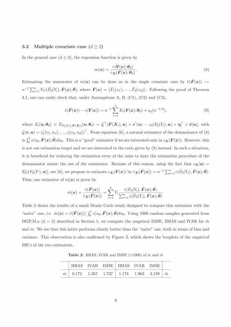
Table 2 shows the results of a small Monte Carlo study designed to compare this estimator with the

“naive” one, i.e. m(x) = e(F (x))/∫ 10 c(u0, F (x); θ)du0. Using 1000 random samples generated from

DGP.M.a (d = 2) described in Section 5, we compute the empirical IMSE, IBIAS and IVAR for m

and m. We see that this latter performs clearly better than the “naive” one, both in terms of bias and

variance. This observation is also confirmed by Figure 2, which shows the boxplots of the empirical

ISE’s of the two estimators.

Table 2: IBIAS, IVAR and IMSE (×1000) of m and m

IBIAS IVAR IMSE IBIAS IVAR IMSE

m 0.172 1.567 1.737 1.178 1.963 3.139 m

9

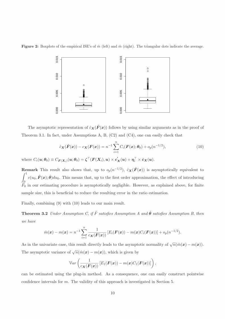
Figure 2: Boxplots of the empirical ISE’s of m (left) and m (right). The triangular dots indicate the average.

0.00

00.

005

0.01

00.

015

0.00

00.

005

0.01

00.

015

The asymptotic representation of cX(F (x)) follows by using similar arguments as in the proof of

Theorem 3.1. In fact, under Assumptions A, B, (C2) and (C4), one can easily check that

cX(F (x))− cX(F (x)) = n−1n∑

i=1

Ci(F (x);θ0) + op(n−1/2), (10)

where Ci(u;θ0) ≡ CF (Xi)(u;θ0) = ζ⊤(F (Xi),u)× c′

X(u) + η⊤

i × cX(u).

Remark This result also shows that, up to op(n−1/2), cX(F (x)) is asymptotically equivalent to

∫ 1

0c(u0, F (x); θ)du0. This means that, up to the first order approximation, the effect of introducing

F0 in our estimating procedure is asymptotically negligible. However, as explained above, for finite

sample size, this is beneficial to reduce the resulting error in the ratio estimation.

Finally, combining (9) with (10) leads to our main result.

Theorem 3.2 Under Assumption C, if F satisfies Assumption A and θ satisfies Assumption B, then

we have

m(x)−m(x) = n−1n∑

i=1

1

cX(F (x))[Ei(F (x))−m(x)Ci(F (x))] + op(n

−1/2).

As in the univariate case, this result directly leads to the asymptotic normality of√n(m(x)−m(x)).

The asymptotic variance of√n(m(x)−m(x)), which is given by

Var

(

1

cX(F (x))[E1(F (x))−m(x)C1(F (x))]

)

,

can be estimated using the plug-in method. As a consequence, one can easily construct pointwise

confidence intervals for m. The validity of this approach is investigated in Section 5.

10

4 Consideration of Misspecification

If the copula family is known, then, as it will be shown in the simulation study, the proposed estimator

is highly accurate. However, in practice, the copula shape is unknown and needs typically to be selected

by the data. Any selection procedure has the possibility that it may select the wrong copula family

in practice. Like any parametric or semiparametric method, using a misspecified (copula) model will

lead to an inconsistent estimator. In this section we are interested in the following question: what

is the effect (cost) of using a misspecified copula model on the resulting regression estimator? Let

C = {c(.;θ), θ ∈ Θ} be any parametric family of copula densities. In the previous sections we assumed

that there exists the true parameter θ0 such that c(.;θ0) coincides with the true copula density, c(·),of (Y,X⊤)⊤. Under a possibly misspecified model, such θ0 may not exist. Instead, we can define θ∗

to be the unique minimum within the set Θ of

I(θ) =

∫

[0,1]d+1

ln

(

c(u0,u)

c(u0,u;θ)

)

dC(u0,u).

This is the classical Kullback-Leibler information criterion expressed in terms of copulas densities

instead of the traditional densities. From the proof of Theorem 3.2, we have the following theorem

regarding the asymptotic behavior of m(x) when the copula family is misspecified.

Theorem 4.1 Under Assumption C, with θ∗ instead of θ0, if F satisfies Assumption A and θ satisfies

Assumption B, with θ∗ instead of θ0, then

m(x)−m(x) =m(x;θ∗)−m(x)

+ n−1n∑

i=1

1

cX(F (x);θ∗)[Ei(F (x);θ∗)−m(x;θ∗)Ci(F (x);θ∗)]

+ op(n−1/2),

where m(x,θ∗) is the mean regression function under the assumption that the joint distribution of

(Y,X⊤)⊤ is C(F0(Y ),F (X);θ∗).

Clearly, when θ∗ = θ0, this theorem reduces to Theorem 3.2. This result also shows that a misspecified

copula brings out a bias in the estimation of m(x), which is asymptotically nothing but the difference

between the true regression function and its best approximation (in terms of likelihood) among the

regression function family {m(x;θ) := E(Y c(F0(Y ),F (x);θ))/cX(F (x);θ), θ ∈ Θ}.

11

Remark Let

θ = argminθ

n∑

i=1

log c

(

n

n+ 1F0(Yi),

n

n+ 1F (Xi);θ

)

be the maximum pseudo-likelihood estimator. By the classical maximum likelihood theory under

misspecification, see White (1982), and following the proof of Theorem 1 in Tsukahara (2005), we

have verified that θ satisfies Assumption B with η as given by (7) but with θ∗ instead of θ0.

5 Simulations

The objective of this section is first to check whether the asymptotic theory for m(x) works both when

the copula is well-specified (Theorem 3.2) and when the copula is misspecified (Theorem 4.1). The

second objective is to compare our semiparametric estimator with some competitors both when the

true copula family is known and when the copula shape is adaptively selected using the data. To this

ends, we consider the following data generating procedures (DGP):

• DGP S.a (F0(Y ), F1(X1)) ∼Gaussian copula with parameter ρ1 = corr(Y,X1); Y ∼ N (µY , σ2Y ).

– The resulting regression function is m(x1) = µY + σY ρ1Φ−1(F1(x1)), where Φ is the c.d.f.

of a standard normal distribution.

– X1 is generated from N (µX1, σ2

X1).

• DGP S.b (F0(Y ), F1(X1)) ∼ FGM copula with parameter θ; Y ∼ N (µY , σ2Y ).

– The resulting regression function is m(x1) =

(

µY − θ√πσY

)

+ 2θ√πσY F1(x1).

– X1 is generated from the c.d.f. FX1(x1) = 1− exp(− exp(x1)).

• DGP S.c (F0(Y ), F1(X1)) ∼ Student t copula with parameters ρ and df ; Y ∼ N (µY , σ2Y ).

– The resulting regression function is

m(x1) = E

{

σY Φ−1(Φdf (ρa+

√

df(1− ρ2)(1 + a2/df)/(df + 1)T )) + µY

}

,

where a = Φ−1df (FX1

(x1)). Φdf is the c.d.f. of a univariate Student t distribution with

degrees of freedom df and T is a univariate Student t random variable with degrees of

freedom df + 1.

– X1 is generated from N (µX1, σ2

X1) .

12

• DGP M.a (F0(Y ), F1(X1), . . . , Fd(Xd)) ∼Gaussian copula with correlation matrix Σ =

1 ρ⊤

ρ ΣX

where ρ = (corr(Y,X1), . . . , corr(Y,Xd))⊤ and ΣX is the d × d correlation matrix of X;

Y ∼ U(0, 1).

– The resulting regression function is m(x) = Φ

d∑

j=1

aj√

1 + (1− ρ⊤a)2Φ−1(Fj(xj))

, where

a = (a1, . . . , ad)⊤ := Σ−1

Xρ.

– Xj is generated from N (µXj, σ2

Xj), j = 1, . . . , d.

• DGP M.b Y = Ψ(−0.3X1+0.9X2+0.3X3)+σǫ, where Ψ is the c.d.f. of the standard Cauchy

distribution.

– X = (X1, X2, X3)⊤ is multivariate normal with mean 0 and Cov(Xi, Xj) = 0.5|i−j|.

– ǫ ∼ N (0, 1) independent of X.

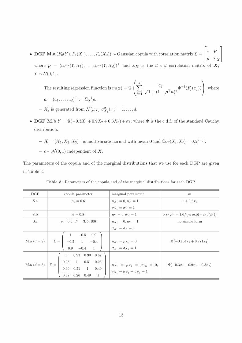
The parameters of the copula and of the marginal distributions that we use for each DGP are given

in Table 3.

Table 3: Parameters of the copula and of the marginal distributions for each DGP.

DGP copula parameter marginal parameter m

S.a ρ1 = 0.6 µX1= 0, µY = 1

σX1= σY = 1

1 + 0.6x1

S.b θ = 0.8 µY = 0, σY = 1 0.8/√

π − 1.6/√

π exp(− exp(x1))

S.c ρ = 0.6, df = 3, 5, 100 µX1= 0, µY = 1

σX1= σY = 1

no simple form

M.a (d = 2) Σ =

1 −0.5 0.9

−0.5 1 −0.4

0.9 −0.4 1

µX1= µX2

= 0

σX1= σX2

= 1

Φ(−0.154x1 + 0.771x2)

M.a (d = 3) Σ =

1 0.23 0.90 0.67

0.23 1 0.51 0.26

0.90 0.51 1 0.49

0.67 0.26 0.49 1

µX1= µX2

= µX3= 0,

σX1= σX2

= σX3= 1

Φ(−0.3x1 + 0.9x2 + 0.3x3)

13

5.1 Verifying asymptotic results

In order to verify the asymptotic results in Section 2 and 3, we draw Quantile-Quantile (Q-Q) plots of

m(x) and calculate empirical coverage probabilities (ECP) of the (1−α)-confidence intervals of m(x)

according to Theorem 3.2 and 4.1. ECP means the proportion of confidence intervals that contain

the true value of the regression function m(x). By seeing whether the ECP’s are close to the nominal

level (1 − α), we can check that the proposed estimator m(x) is asymptotically normal. Also, we

can validate the asymptotic i.i.d. representation for m(x) and the appropriateness of the proposed

variance estimator of m(x). We calculate the estimator m(x) from N = 1000 random samples of size

n = 50, 100, 200 and 400. This is done for different values of significance level α and points of interest

x. Only selected and representative results are shown to save space and avoid repetition.

When the copula is well-specified

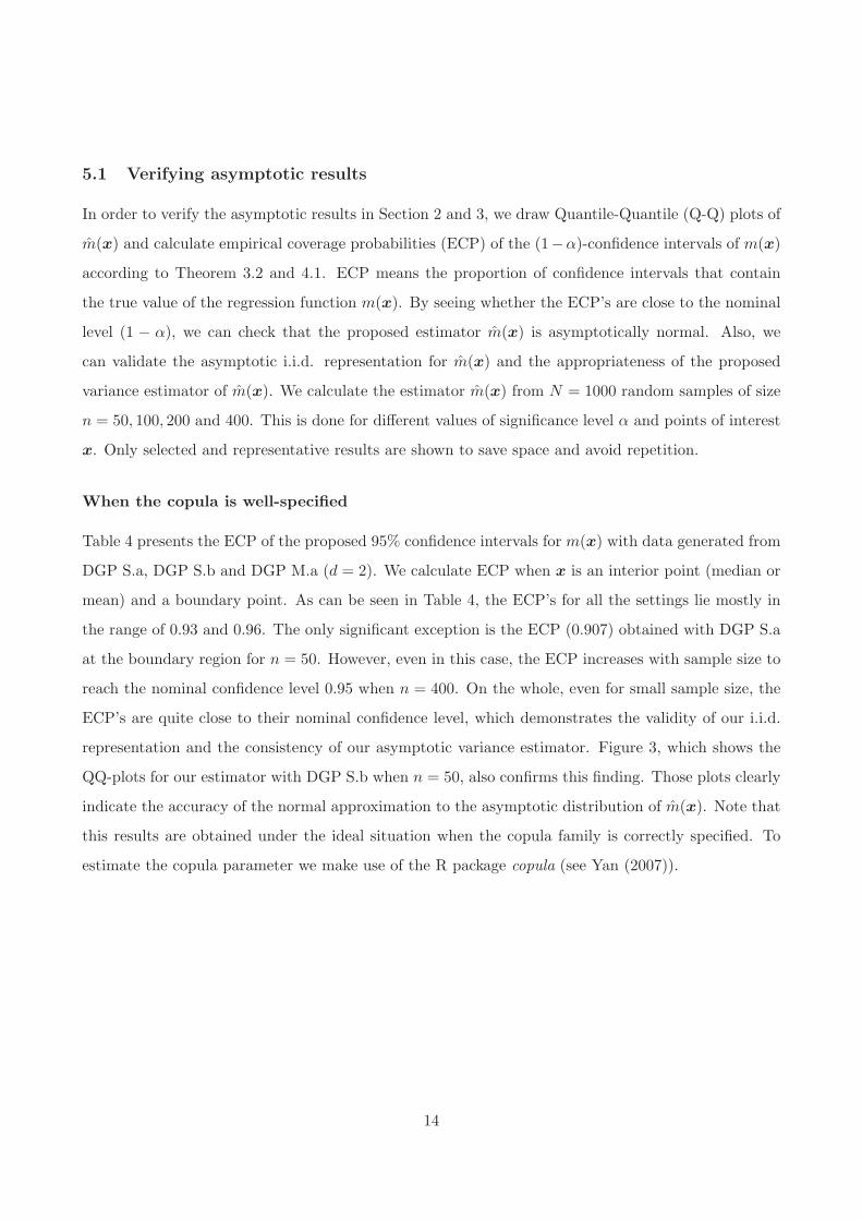
Table 4 presents the ECP of the proposed 95% confidence intervals for m(x) with data generated from

DGP S.a, DGP S.b and DGP M.a (d = 2). We calculate ECP when x is an interior point (median or

mean) and a boundary point. As can be seen in Table 4, the ECP’s for all the settings lie mostly in

the range of 0.93 and 0.96. The only significant exception is the ECP (0.907) obtained with DGP S.a

at the boundary region for n = 50. However, even in this case, the ECP increases with sample size to

reach the nominal confidence level 0.95 when n = 400. On the whole, even for small sample size, the

ECP’s are quite close to their nominal confidence level, which demonstrates the validity of our i.i.d.

representation and the consistency of our asymptotic variance estimator. Figure 3, which shows the

QQ-plots for our estimator with DGP S.b when n = 50, also confirms this finding. Those plots clearly

indicate the accuracy of the normal approximation to the asymptotic distribution of m(x). Note that

this results are obtained under the ideal situation when the copula family is correctly specified. To

estimate the copula parameter we make use of the R package copula (see Yan (2007)).

14

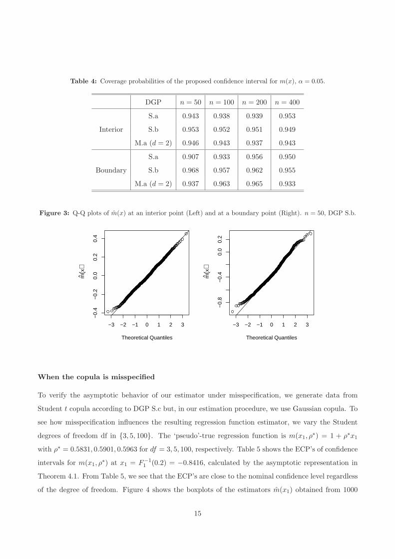
Table 4: Coverage probabilities of the proposed confidence interval for m(x), α = 0.05.

DGP n = 50 n = 100 n = 200 n = 400

Interior

S.a 0.943 0.938 0.939 0.953

S.b 0.953 0.952 0.951 0.949

M.a (d = 2) 0.946 0.943 0.937 0.943

Boundary

S.a 0.907 0.933 0.956 0.950

S.b 0.968 0.957 0.962 0.955

M.a (d = 2) 0.937 0.963 0.965 0.933

Figure 3: Q-Q plots of m(x) at an interior point (Left) and at a boundary point (Right). n = 50, DGP S.b.

−3 −2 −1 0 1 2 3

−0.

4−

0.2

0.0

0.2

0.4

Theoretical Quantiles

m(x

)

−3 −2 −1 0 1 2 3

−0.

8−

0.4

0.0

0.2

Theoretical Quantiles

m(x

)

When the copula is misspecified

To verify the asymptotic behavior of our estimator under misspecification, we generate data from

Student t copula according to DGP S.c but, in our estimation procedure, we use Gaussian copula. To

see how misspecification influences the resulting regression function estimator, we vary the Student

degrees of freedom df in {3, 5, 100}. The ‘pseudo’-true regression function is m(x1, ρ∗) = 1 + ρ∗x1

with ρ∗ = 0.5831, 0.5901, 0.5963 for df = 3, 5, 100, respectively. Table 5 shows the ECP’s of confidence

intervals for m(x1, ρ∗) at x1 = F−1

1 (0.2) = −0.8416, calculated by the asymptotic representation in

Theorem 4.1. From Table 5, we see that the ECP’s are close to the nominal confidence level regardless

of the degree of freedom. Figure 4 shows the boxplots of the estimators m(x1) obtained from 1000

15

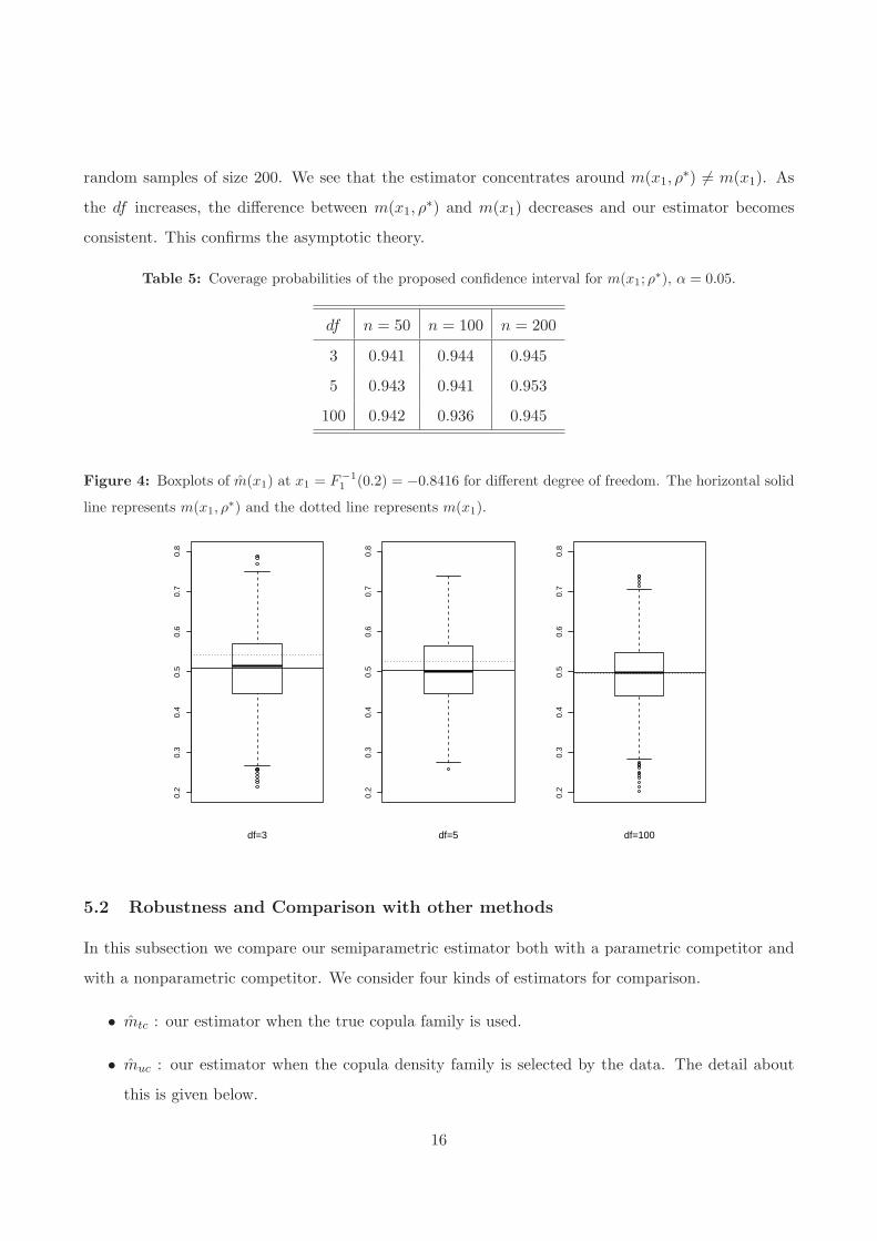
random samples of size 200. We see that the estimator concentrates around m(x1, ρ∗) 6= m(x1). As

the df increases, the difference between m(x1, ρ∗) and m(x1) decreases and our estimator becomes

consistent. This confirms the asymptotic theory.

Table 5: Coverage probabilities of the proposed confidence interval for m(x1; ρ∗), α = 0.05.

df n = 50 n = 100 n = 200

3 0.941 0.944 0.945

5 0.943 0.941 0.953

100 0.942 0.936 0.945

Figure 4: Boxplots of m(x1) at x1 = F−1

1(0.2) = −0.8416 for different degree of freedom. The horizontal solid

line represents m(x1, ρ∗) and the dotted line represents m(x1).

0.2

0.3

0.4

0.5

0.6

0.7

0.8

df=3

0.2

0.3

0.4

0.5

0.6

0.7

0.8

df=5

0.2

0.3

0.4

0.5

0.6

0.7

0.8

df=100

5.2 Robustness and Comparison with other methods

In this subsection we compare our semiparametric estimator both with a parametric competitor and

with a nonparametric competitor. We consider four kinds of estimators for comparison.

• mtc : our estimator when the true copula family is used.

• muc : our estimator when the copula density family is selected by the data. The detail about

this is given below.

16

• mls : parametric regression estimator based on the classical least square method.

• mll : nonparametric regression estimator (local linear).

As a comparison criterion we calculate the empirical Integrated Mean Squared Error (IMSE) given by

IMSE =1

N

N∑

j=1

ISE(m(j)) :=1

N

N∑

j=1

[

1

I

I∑

i=1

(

m(j)(xi)−m(xi))2

]

(11)

=1

I

I∑

i=1

(

m(xi)− ¯m(xi))2

+1

I

I∑

i=1

1

N

N∑

j=1

(m(j)(xi)− ¯m(xi))2

≡ IBIAS2 + IVAR.

where {xi, i = 1, . . . , I} is the fixed evaluation set which corresponds to a random sample of size

I = 500 from the distribution of X, m(j)(·) is the estimated regression function from the j-th data

sample and ¯m(xi) = N−1∑N

j=1 m(j)(xi).

Single covariate case

In order to compute the estimator muc, we should decide which copula family to use and then estimate

its parameters. In our simulations, we use AIC criterion to select one bivariate copula family among ten

candidates: two are elliptical (Gaussian and Student t) and eight are Archimedean (Clayton, Gumbel,

Frank, Joe, Clayton-Gumbel, Joe-Gumbel, Joe-Clayton and Joe-Frank). See, e.g., Brechmann and

Schepsmeier (2011) for the definition of all these copulas.

The data was generated from FGM copula according to DGP S.b. The regression function is

given by m(x1) = 0.8/√π − 1.6/

√π exp(− exp(x1). To calculate mtc we use the FGM copula. Note

that the true copula is not included in the list of ten candidate copulas families cited above and so

the misspecified copula based estimator muc is expected to behave badly compared to mtc. As a

parametric regression model we use the true regression function a exp(− exp(bx1)) + c. To calculate

mls, we estimate a, b and c by the non-linear least squared method using the R package nlrwr. For

details, we refer to Ritz and Streibig (2008). We also make use of the R package np to calculate mll;

see Hayfield and Racine (2008). The bandwidth parameter is selected via the cross-validation method.

The obtained results (see Table 6) of this study are better than what we expected. In fact, in

terms of mean squared error, our estimator beats not only the local linear estimator but also the

least squared estimator even when the copula distribution is unknown and selected (incorrectly) by

the data. There are two reasons that may explain such a result. The first is that the classical least

17

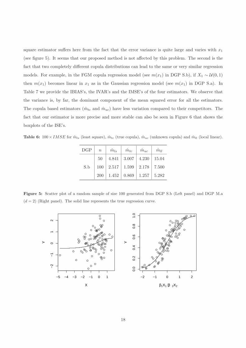
square estimator suffers here from the fact that the error variance is quite large and varies with x1

(see figure 5). It seems that our proposed method is not affected by this problem. The second is the

fact that two completely different copula distributions can lead to the same or very similar regression

models. For example, in the FGM copula regression model (see m(x1) in DGP S.b), if X1 ∼ U(0, 1)then m(x1) becomes linear in x1 as in the Gaussian regression model (see m(x1) in DGP S.a). In

Table 7 we provide the IBIAS’s, the IVAR’s and the IMSE’s of the four estimators. We observe that

the variance is, by far, the dominant component of the mean squared error for all the estimators.

The copula based estimators (mtc and muc) have less variation compared to their competitors. The

fact that our estimator is more precise and more stable can also be seen in Figure 6 that shows the

boxplots of the ISE’s.

Table 6: 100× IMSE for mls (least square), mtc (true copula), muc (unknown copula) and mll (local linear).

DGP n mls mtc muc mll

S.b

50 4.841 3.007 4.230 15.04

100 2.517 1.599 2.178 7.500

200 1.452 0.869 1.257 5.282

Figure 5: Scatter plot of a random sample of size 100 generated from DGP S.b (Left panel) and DGP M.a

(d = 2) (Right panel). The solid line represents the true regression curve.

−5 −4 −3 −2 −1 0 1

−2

−1

01

2

X

Y

−2 −1 0 1 2

0.0

0.2

0.4

0.6

0.8

1.0

β1X1 + β2X2

Y

18

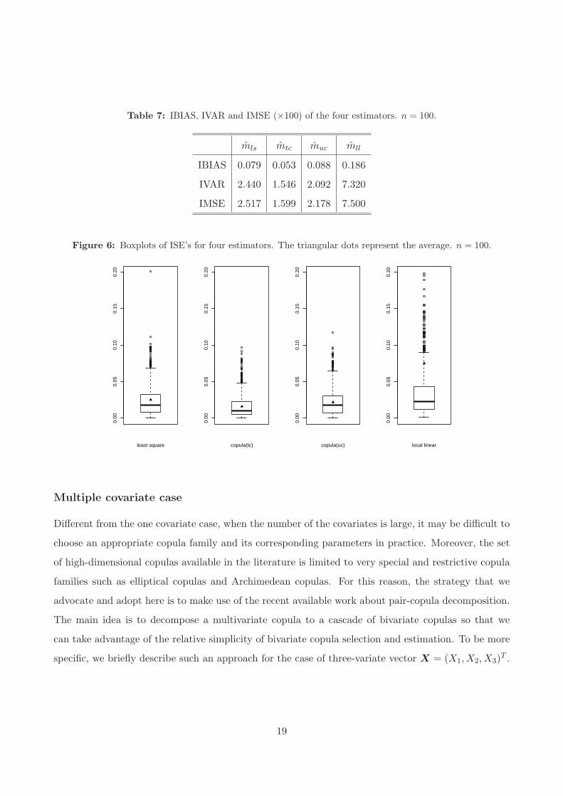
Table 7: IBIAS, IVAR and IMSE (×100) of the four estimators. n = 100.

mls mtc muc mll

IBIAS 0.079 0.053 0.088 0.186

IVAR 2.440 1.546 2.092 7.320

IMSE 2.517 1.599 2.178 7.500

Figure 6: Boxplots of ISE’s for four estimators. The triangular dots represent the average. n = 100.

0.00

0.05

0.10

0.15

0.20

least square

0.00

0.05

0.10

0.15

0.20

copula(tc)

0.00

0.05

0.10

0.15

0.20

copula(uc)

0.00

0.05

0.10

0.15

0.20

local linear

Multiple covariate case

Different from the one covariate case, when the number of the covariates is large, it may be difficult to

choose an appropriate copula family and its corresponding parameters in practice. Moreover, the set

of high-dimensional copulas available in the literature is limited to very special and restrictive copula

families such as elliptical copulas and Archimedean copulas. For this reason, the strategy that we

advocate and adopt here is to make use of the recent available work about pair-copula decomposition.

The main idea is to decompose a multivariate copula to a cascade of bivariate copulas so that we

can take advantage of the relative simplicity of bivariate copula selection and estimation. To be more

specific, we briefly describe such an approach for the case of three-variate vector X = (X1, X2, X3)T .

19

By applying Sklar’s theorem recursively one can write (for example)

c(F0(y), F1(x1), F2(x2), F3(x3)) =cX(F1(x1), F2(x2), F3(x3))× c01(F0(y), F1(x1))×

c02|1(F0|1(y|x1), F2|1(x2|x1)|x1)× (12)

c03|12(F0|12(y|x1, x2), F3|12(x3|x1, x2)|x1, x2),

where c01, c02|1 and c03|12 are the copula densities associated with the distributions of (Y,X1),

(Y,X2)|X1 and (Y,X3)|(X1, X2) , respectively. Similarly, cX can be, for example, decomposed as

cX(F1(x1), F2(x2), F3(x3)) = c12(F1(x1), F2(x2))×c23(F2(x2), F3(x3))×c13|2(F1|2(x1|x2), F3|2(x3|x2);x2).If we assume that all the conditional copulas depend on the conditioning variables only through the

conditional distributions, e.g. c02|1(F0|1(y|x1), F2|1(x2|x1)|x1) = c02|1(F0|1(y|x1), F2|1(x2|x1)), then it

leads to the so-called simplified pair-copula decomposition. Because any bivariate copula family could

be used as a building block for this decomposition, the simplified pair-copula decomposition provides

high flexibility and the ability to cover a wide range of complex dependencies. In our simulation, we

consider all the possible pair-copula decompositions with ten candidate bivariate copulas and choose

one decomposition (vine structure) which maximizes the AIC criterion. Hobæk Haff et al. (2010)

discussed the conditions under which such a simplification is possible and found that this is not a

severe restriction in many situations. For more about vines see the recent book by Kurowicka and

Joe (2010). The problem of selecting an appropriate simplified decomposition and an appropriate

parametric shape of each pair-copula and the estimation of the copula parameters are discussed in,

e.g., Aas et al. (2009), Kurowicka and Joe (2010), Hobæk Haff (2012) and the references given there.

Remark Observe that the equality (12) holds without any restrictions in the copula c. As a conse-

quence, by (1), the regression function can also be express as

m(x1, x2, x3) =E(Y × c01(F0(Y ), F1(x1))× c02|1(F0|1(Y |x1), F2|1(x2|x1)|x1)×

c03|12(F0|12(Y |x1, x2), F3|12(x3|x1, x2)|x1, x2)).

Assuming that the pair simplifications holds, then one can use this equality to define a new class of

estimation method. This approach will not be investigated in the current work.

We generate data according to DGP M.a (d = 2) and M.a (d = 3). Figure 5 shows the scatter

plot of Y versus −0.154X1 + 0.771X2 using one random sample generated from DGP M.a (d = 2).

To calculate muc, the pair-copulas in each candidate decomposition are also selected using the AIC

20

criterion as in the one covariate case. We estimate the copula parameters by the maximum pseudo-

likelihood method. All the computations are done via the R package CDVine (see Brechmann and

Schepsmeier (2011)). As a parametric competitor we consider the nonlinear least square estimators

from the model m(x1, x2) = Φ(β1x1 + β2x2) when d = 2 and m(x1, x2, x3) = Φ(β1x1 + β2x2 + β3x3)

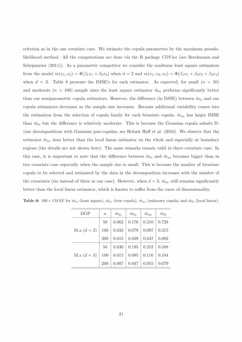
when d = 3. Table 8 presents the IMSE’s for each estimator. As expected, for small (n = 50)

and moderate (n = 100) sample sizes the least square estimator mls performs significantly better

than our semiparametric copula estimators. However, the difference (in IMSE) between mls and our

copula estimators decreases as the sample size increases. Because additional variability comes into

the estimation from the selection of copula family for each bivariate copula, muc has larger IMSE

than mtc but the difference is relatively moderate. This is because the Gaussian copula admits D-

vine decompositions with Gaussian pair-copulas; see Hobæk Haff et al. (2010). We observe that the

estimator muc does better than the local linear estimator on the whole and especially at boundary

regions (the details are not shown here). The same remarks remain valid in three covariate case. In

this case, it is important to note that the difference between mtc and muc becomes bigger than in

two covariate case especially when the sample size is small. This is because the number of bivariate

copula to be selected and estimated by the data in the decomposition increases with the number of

the covariates (six instead of three in our case). However, when d = 3, muc still remains significantly

better than the local linear estimator, which is known to suffer from the curse of dimensionality.

Table 8: 100× IMSE for mls (least square), mtc (true copula), muc (unknown copula) and mll (local linear).

DGP n mls mtc muc mll

M.a (d = 2)

50 0.062 0.176 0.210 0.728

100 0.032 0.079 0.097 0.215

200 0.015 0.039 0.047 0.092

M.a (d = 3)

50 0.030 0.195 0.252 0.588

100 0.015 0.095 0.116 0.184

200 0.007 0.047 0.055 0.079

21

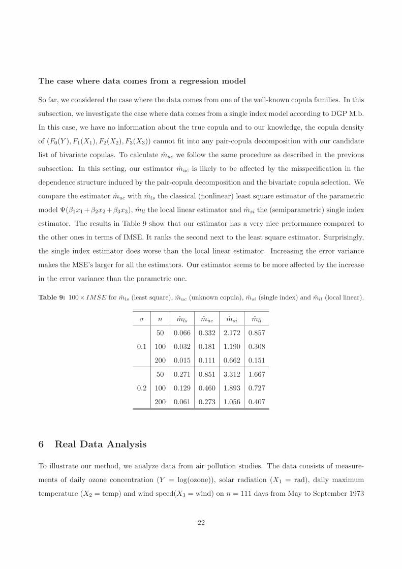
The case where data comes from a regression model

So far, we considered the case where the data comes from one of the well-known copula families. In this

subsection, we investigate the case where data comes from a single index model according to DGP M.b.

In this case, we have no information about the true copula and to our knowledge, the copula density

of (F0(Y ), F1(X1), F2(X2), F3(X3)) cannot fit into any pair-copula decomposition with our candidate

list of bivariate copulas. To calculate muc we follow the same procedure as described in the previous

subsection. In this setting, our estimator muc is likely to be affected by the misspecification in the

dependence structure induced by the pair-copula decomposition and the bivariate copula selection. We

compare the estimator muc with mls the classical (nonlinear) least square estimator of the parametric

model Ψ(β1x1+β2x2+β3x3), mll the local linear estimator and msi the (semiparametric) single index

estimator. The results in Table 9 show that our estimator has a very nice performance compared to

the other ones in terms of IMSE. It ranks the second next to the least square estimator. Surprisingly,

the single index estimator does worse than the local linear estimator. Increasing the error variance

makes the MSE’s larger for all the estimators. Our estimator seems to be more affected by the increase

in the error variance than the parametric one.

Table 9: 100× IMSE for mls (least square), muc (unknown copula), msi (single index) and mll (local linear).

σ n mls muc msi mll

0.1

50 0.066 0.332 2.172 0.857

100 0.032 0.181 1.190 0.308

200 0.015 0.111 0.662 0.151

0.2

50 0.271 0.851 3.312 1.667

100 0.129 0.460 1.893 0.727

200 0.061 0.273 1.056 0.407

6 Real Data Analysis

To illustrate our method, we analyze data from air pollution studies. The data consists of measure-

ments of daily ozone concentration (Y = log(ozone)), solar radiation (X1 = rad), daily maximum

temperature (X2 = temp) and wind speed(X3 = wind) on n = 111 days from May to September 1973

22

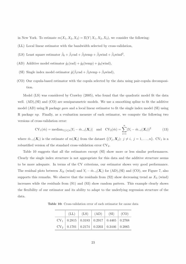
in New York. To estimate m(X1, X2, X3) = E(Y |X1, X2, X3), we consider the following:

(LL) Local linear estimator with the bandwidth selected by cross-validation,

(LS) Least square estimator β0 + β1rad + β2temp + β3wind + β4wind2,

(AD) Additive model estimator g1(rad) + g2(temp) + g3(wind),

(SI) Single index model estimator g(β1rad + β2temp + β3wind),

(CO) Our copula-based estimator with the copula selected by the data using pair-copula decomposi-

tion.

Model (LS) was considered by Crawley (2005), who found that the quadratic model fit the data

well. (AD),(SI) and (CO) are semiparametric models. We use a smoothing spline to fit the additive

model (AD) using R package gam and a local linear estimator to fit the single index model (SI) using

R package np. Finally, as a evaluation measure of each estimator, we compute the following two

versions of cross-validation error:

CV1(m) = median1≤i≤n|Yi − m−i(Xi)| and CV2(m) =

n∑

i=1

(Yi − m−i(Xi))2 (13)

where m−i(Xi) is the estimate of m(Xi) from the dataset {(Yj ,Xj); j 6= i, j = 1, . . . , n}. CV1 is a

robustified version of the standard cross-validation error CV2.

Table 10 suggests that all the estimators except (SI) show more or less similar performances.

Clearly the single index structure is not appropriate for this data and the additive structure seems

to be more adequate. In terms of the CV criterions, our estimator shows very good performance.

The residual plots between X3i (wind) and Yi − m−i(Xi) for (AD),(SI) and (CO), see Figure 7, also

supports this remarks. We observe that the residuals from (S2) show decreasing trend as X3 (wind)

increases while the residuals from (S1) and (S3) show random pattern. This example clearly shows

the flexibility of our estimator and its ability to adapt to the underlying regression structure of the

data.

Table 10: Cross-validation error of each estimator for ozone data

(LL) (LS) (AD) (SI) (CO)

CV1 0.2815 0.3183 0.2917 0.4465 0.2768

CV2 0.1701 0.2174 0.2203 0.3446 0.2065

23

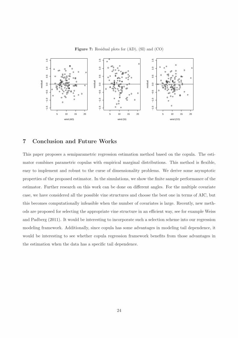
Figure 7: Residual plots for (AD), (SI) and (CO)

5 10 15 20

−1.

5−

1.0

−0.

50.

00.

51.

01.

5

wind (AD)

resi

dual

5 10 15 20

−1.

5−

1.0

−0.

50.

00.

51.

01.

5

wind (SI)

resi

dual

5 10 15 20

−1.

5−

1.0

−0.

50.

00.

51.

01.

5

wind (CO)

resi

dual

7 Conclusion and Future Works

This paper proposes a semiparametric regression estimation method based on the copula. The esti-

mator combines parametric copulas with empirical marginal distributions. This method is flexible,

easy to implement and robust to the curse of dimensionality problems. We derive some asymptotic

properties of the proposed estimator. In the simulations, we show the finite sample performance of the

estimator. Further research on this work can be done on different angles. For the multiple covariate

case, we have considered all the possible vine structures and choose the best one in terms of AIC, but

this becomes computationally infeasible when the number of covariates is large. Recently, new meth-

ods are proposed for selecting the appropriate vine structure in an efficient way, see for example Weiss

and Padberg (2011). It would be interesting to incorporate such a selection scheme into our regression

modeling framework. Additionally, since copula has some advantages in modeling tail dependence, it

would be interesting to see whether copula regression framework benefits from those advantages in

the estimation when the data has a specific tail dependence.

24

Appendix

Proof of Theorem 3.1

Using Taylor expansion, we have

m(x1) = n−1n∑

i=1

Yic(F0(Yi), F1(x1);θ0) + V1 + V2 + V3,

where

V1 = n−1n∑

i=1

Yi(F0(Yi)− F0(Yi)) c0(ui,0, u1; θ), V2 = n−1n∑

i=1

Yi(F1(x1)− F1(x1)) c1(ui,0, u1; θ),

V3 = n−1n∑

i=1

Yi(θ − θ0)⊤ c(u0,i, u1; θ)

with ui,0 = F0(Yi) + t(F0(Yi)− F0(Yi)), u1 = F1(x1) + t(F1(x1)− F1(x1)) and θ = θ0 + t(θ − θ0) for

some t ∈ [0, 1]. Using Taylor expansion again, V1 can be represented as

V1 = n−1n∑

i=1

Yi(F0(Yi)− F0(Yi)) c0(F0(Yi), F1(x1);θ0) +R1,

where

R1 = n−1n∑

i=1

Yi(F0(Yi)− F0(Yi))[c0(ui,0, u1; θ)− c0(F0(Yi), F1(x1);θ0)].

By Assumption (C1)(i) and (C2) and the compactness of Θ, we have

|R1| ≤ supi

|F0(Yi)− F0(Yi)| supi

|c0(ui,0, u1; θ)− c0(F0(Yi), F1(x1);θ0)|n−1n∑

i=1

|Yi|

= Op(n−1/2)op(1)Op(1) = op(n

−1/2),

which leads to V1 = V1+op(n−1/2) with V1 = n−1

∑ni=1 Yi(F0(Yi)−F0(Yi))c0(F0(Yi), F1(x1)). Similarly,

we know that V2 = V2 + op(n−1/2) with V2 = n−1

∑ni=1 Yi(F1(x) − F1(x))c1(F0(Yi), F1(x1)), and also

that V3 = V3 + op(n−1/2) with V3 = n−1

∑ni=1 Yi(θ − θ0)

⊤c(F0(Yi), F1(x1)) using θ − θ0 = Op(n−1/2)

in Assumption B. Summing up the results until now, we conclude

m(x1) = n−1n∑

i=1

Yic(F0(Yi), F1(x1)) + V1 + V2 + V3 + op(n−1/2) (14)

By Assumption (A) and (C4),

V2 = n−1n∑

i=1

ζ(F1(Xi,1), F1(x1))× e1(F1(x1)) + op(n−1/2) (15)

25

Note that V1 is a V -statistic with the kernel

h1(Yi, Yj) =1

2[Yi(I(Yj ≤ Yi)− F0(Yi))c0(F0(Yi), F1(x1)) + Yj(I(Yi ≤ Yj)− F0(Yj))c0(F0(Yj), F1(x1))].

By Assumption (C4), using the fact that Eh1(Yi, Yj) = 0 and the classical V -statistic techniques ( see

e.g. Serfling (1980)), we obtain that

V1 = n−1n∑

i=1

λ(Yi, F1(x1)) + op(n−1/2), (16)

where λ(t, u1) = E[Y (I(t ≤ Y )−F0(Y ))c0(F0(Y ), u1)]. Further, V3 is also a V -statistic with the kernel

h3((Xi,1, Yi)⊤, (Xj,1, Yj)

⊤) =1

2[Yiη

⊤j × c(F0(Yi), F1(x1)) + Yjη

⊤i × c(F0(Yj), F1(x1))].

By Assumption (B) and (C4) we obtain that

V3 = n−1n∑

i=1

η⊤i × e(F1(x1)) + op(n

−1/2). (17)

From (14)-(17), we know that

m(x1) = n−1n∑

i=1

[Yic(F0(Yi), F1(x1)) + λ(Yi, F1(x1)) + ζ(F1(Xi,1), F1(x1))× e1(F1(x1))+

η⊤(F0(Yi), F1(Xi,1))× e(F1(x1))] + op(n−1/2),

This combined with the fact λ(t, u1) = E[Y c(F0(Y ), u1)]−tc(F0(t), u1)−∫

(I(t ≤ y)−F0(y))c(F0(y), u1)dy

from Assumption (C1) concludes the proof.

References

K. Aas, C. Czado, A. Frigessi, and H. Bakken. Pair-copula constructions of multiple dependence.

Insurance: Mathematics and Economics, 44:182–198, 2009.

T. Bouezmarni, J. V. K. Rombouts, and A. Taamouti. Asymptotic properties of the bernstein density

copula estimator for α-mixing data. Journal of Multivariate Analysis, 101:1 – 10, 2010.

E. Brechmann and U. Schepsmeier. Modeling dependence with C-and D-vine copulas: The R-package

CDVine. Technical report, 2011.

A. Charpentier, J.-D. Fermanian, and O. Scaillet. Copulas: From theory to application in finance,

chapter The Estimation of Copulas: Theory and Practice. Risk Publications, London, 2006.

26

S. X. Chen and T.-M. Huang. Nonparametric estimation of copula functions for dependence modelling.

Canadian Journal of Statistics, 35:265–282, 2007.

G. J. Crane and J. Van Der Hoek. Conditional Expectation Formulae for Copulas. Australian and

New Zealand Journal of Statistics, 50:53–67, 2008.

M. J. Crawley. Statistics: An Introduction using R. John Wiley & Sons, Ltd., 2005.

C. Genest, K. Ghoudi, and L. Rivest. A semiparametric estimation procedure of dependence param-

eters in multivariate families of distributions. Biometrika, 82:543–552, 1995.

I. Gijbels and J. Mielniczuk. Estimating the density of a copula function. Communications in Statistics

- Theory and Methods, 19:445–464, 1990.

T. Hayfield and J. S. Racine. Nonparametric econometrics: The np package. Journal of Statistical

Software, 27, 2008.

I. Hobæk Haff. Parameter estimation for pair-copula constructions. Bernoulli, to appear, 2012.

I. Hobæk Haff, K. Aas, and A. Frigessi. On the simplified pair-copula construction - Simply useful or

too simplistic? Journal of Multivariate Analysis, 101:1296–1310, 2010.

I. Kojadinovic and J. Yan. A goodness-of-fit test for multivariate multiparameter copulas based on

multiplier central limit theorems. Statistics and Computing, 21:17–30, 2011.

D. Kurowicka and H. Joe, editors. Dependence Modeling: Vine Copula Handbook. World Scientific

Books. World Scientific Publishing Co. Pte. Ltd., 2010.

Y. K. Leong and E. A. Valdez. Claims Prediction with Dependence using Copula Models. Technical

report, 2005.

R. B. Nelsen. An introduction to copulas. Springer Series in Statistics. Springer, New York, 2006.

C. Ritz and J. C. Streibig. Nonlinear Regression in R. Springer, 2008.

R. J. Serfling. Approximation theorems of mathematical statistics. John Wiley & Sons Inc., 1980.

Wiley Series in Probability and Mathematical Statistics.

P. Silvapulle, G. Kim, and M. J. Silvapulle. Robustness of a semiparametric estimator of a copula.

Econometric Society 2004 Australasian Meetings 317, Econometric Society, 2004.

27

M. Sklar. Fonctions de repartition a n dimensions et leurs marges. Publ. Inst. Statist. Univ. Paris, 8:

229–231, 1959.

E. A. Sungur. Some Observations on Copula Regression Functions. Communications in Statistics-

Theory and Methods, 34:1967–1978, 2005.

H. Tsukahara. Semiparametric estimation in copula models. Canadian Journal of Statistics, 33:

357–375, 2005.

G. Weiss and M. Padberg. Automated vine copula calibration using genetic algorithms. Technical

report, TU Dortmund University, 2011.

H. White. Maximum likelihood estimation of misspecified models. Econometrica, 50:1–25, 1982.

J. Yan. Enjoy the Joy of Copulas : With a Package copula. Journal of Statistical Software, 21, 2007.

28