capacity planning and sizing for microsoft sharepoint … planning and sizing for microsoft...

Capacity Planning and Sizing for Microsoft SharePoint Server 2010 Based Divisional Portal

This document is provided “as-is”. Information and views expressed in this document, including URL and

other Internet Web site references, may change without notice. You bear the risk of using it.

Some examples depicted herein are provided for illustration only and are fictitious. No real association

or connection is intended or should be inferred.

This document does not provide you with any legal rights to any intellectual property in any Microsoft

product. You may copy and use this document for your internal, reference purposes.

© 2010 Microsoft Corporation. All rights reserved.

Capacity Planning and Sizing for Microsoft SharePoint Server 2010 Based Divisional Portal

Gaurav Doshi, Raj Dhrolia, Wayne Roseberry

Microsoft Corporation

February 2010

Applies to: Office SharePoint Server 2010

Summary: This whitepaper provides guidance on performance and capacity planning for a

SharePoint Server 2010 based divisional portal.

Test environment specifications, such as hardware, farm topology and configuration;

Test farm dataset;

Test data and recommendations for how to determine the hardware, topology and

configuration you need to deploy a similar environment, and how to optimize your

environment for appropriate capacity and performance characteristics.

Table of Contents Introduction .................................................................................................................................................. 4

Scenario ..................................................................................................................................................... 4

Assumptions and prerequisites................................................................................................................. 4

Test setup ..................................................................................................................................................... 6

Hardware................................................................................................................................................... 6

Software .................................................................................................................................................... 6

Topology and configuration ...................................................................................................................... 7

Dataset and disk geometry ....................................................................................................................... 8

Transactional mix ...................................................................................................................................... 9

Results and analysis ................................................................................................................................... 11

Test methodology ................................................................................................................................... 11

Results from iterations (1 X 1, 1 X 1 X 1, 2 X 1 X 1, 3 X 1 X 1) ................................................................. 12

1 X 1 farm configuration ................................................................................................................ 12

1 X 1 X 1 farm configuration .......................................................................................................... 13



Comparison ............................................................................................................................................ 19

Tests with Search incremental crawl ...................................................................................................... 21

Summary of results and recommendations ........................................................................................... 22

Introduction

Scenario

This document outlines the test methodology and results to provide guidance for capacity planning of a typical divisional portal. A divisional portal is a Microsoft® SharePoint® Server 2010 deployment where teams mainly do collaborative activities and some content publishing. This document assumes a “division” to be an organization within an enterprise with 1,000 to 10,000 employees.

Different scenarios will have different requirements, so it is important to supplement this guidance with

additional testing on your own hardware and in your own environment.

When you read this document, you will understand how to:

Estimate the hardware required to support the scale you need to support: number of users,

load, and the features enabled.

Design your physical and logical topology for optimum reliability and efficiency. High

Availability/Disaster Recovery are not covered in this document.

Impact of ongoing search crawl on RPS of a divisional portal like deployment

Before you read this document, you should read the following:

Capacity Planning and Sizing for Microsoft SharePoint 2010 Products and Technologies

Office SharePoint Server 2010 Software Boundaries

Also, you may want to read the following:

“Microsoft SharePoint Server 2010 Departmental Collaboration Environment” document from

the Performance and capacity technical case studies page (http://technet.microsoft.com/en-

us/library/cc261716(office.14).aspx).

Assumptions and prerequisites

In the scope of this testing, we did not consider disk I/O as a limiting factor. It is assumed that

infinite numbers of spindles are available.

The tests only model peak time usage on a typical divisional portal. We did not consider cyclical

changes in traffic seen with day-night cycles. That also means that timer jobs which require

generally scheduled nightly run are not included in the mix.

There is no custom code running on the divisional portal deployment in this case. We cannot

guarantee behavior of custom code/third party solutions installed on top of your divisional

portal.

http://technet.microsoft.com/en-us/library/cc261716(office.14).aspx

For the purpose of tests, all the services DBs and content DB were placed on the same instance

of Microsoft SQL Server®. Also, Usage DB was maintained on a separate instance of SQL Server.

For the purpose of tests, BLOB cache is enabled

Authentication mode was NTLM

Search crawl traffic is not taken into consideration in these tests. But to factor in impact of an

ongoing search crawl, we modified definitions of a healthy farm. (Green-zone definition to be 40

percent for SQL Server to allow 10 percent tax from Search crawls. Similarly, we used 80 percent

SQL Server CPU as the criteria for max RPS.)

Test setup

Hardware

The table below presents hardware specs for the computers used in this testing. Every front-end Web

server that was added to the server farm during multiple iterations of the test complies to the same

specs.

Front-end Web server

Application Server Database Server

Server model PE 2950 PE 2950 Dell PE 6850

Processor(s) [email protected] [email protected] 4px4c@ 3.19GHz

RAM 8 GB 8 GB 32 GB

# of NICs 2 2 1

NIC speed 1 gigabit 1 gigabit 1 gigabit

Load balancer type F5 - Hardware load balancer

n/a n/a

ULS Logging level Medium Medium n/a

Table 1: Hardware specifications for server computers

Software Table below explains software installed and running on the servers used in this testing effort.

Front-end Web Server Application Server Database Server

Operating System

Windows Server® 2008 R2 x64

Windows Server 2008 R2 x64

Windows Server 2008 x64

Software version

Microsoft SharePoint 4733.1000, WAC 4733.1000

Microsoft SharePoint 4733.1000, WAC 4733.1000

SQL Server 2008 R2 CTP3

Load balancer type

F5 - Hardware load balancer

n/a n/a

ULS Logging level

Medium Medium n/a

Anti-Virus Settings

Disabled Disabled Disabled

Table 2: Software specifications for server computers

Topology and configuration The topology diagram below explains hardware setup used for the tests. We changed the number of

front-end Web servers from 1 to 2 to 3, as we moved between iterations, but otherwise the topology

remained the same.

Diagram 1: Farm Configuration

Please refer to the diagram above for the services which are provisioned in the test environment. Other

Services such as User Profile Service and Web Analytics are not provisioned.

Dataset and disk geometry Test farm was populated with around 1.62 terabytes of content, distributed across 5 different sized

content databases. The table below explains this distribution:

Content DB # 1 2 3 4 5

Content DB size

36 GB 135 GB 175 GB 1.2 terabytes 75 GB

# of sites 44 74 9 9 222

# of Webs 1544 2308 2242 2041 1178

RAID configuration

0 0 0 0 0

# of spindles for MDF

1 1 5 3 1

# of spindles for LDF

1 1 1 1 1

Table 3: Dataset and disk geometry

Transactional mix Important notes

There are no My Sites provisioned on the divisional portal. Also, User Profile Service, which

supports My Sites is not running on the farm. Transactional mix does not include any My Site

page/web service hits or traffic related to Outlook Social Connector.

Test mix does not include any traffic generated by co-authoring on documents.

Test mix does not include traffic from Search Crawl. However this was factored into our tests by

modifying the Green-zone definition to be 40 percent SQL Server CPU usage as opposed to the

standard 50 percent to allow 10 percent for the search crawl. Similarly, we used 80 percent SQL

Server CPU as the criteria for max RPS.

Overall transaction mix is presented below in a table

Feature /Service Operation Read/write % of mix

ECM Get static files r 8.93%

View homepage r 1.52%

Microsoft Infopath® Display/Edit upsize list item and new forms r 0.32%

Download file, using 'save as' r 1.39%

Microsoft Onenote® Open O12 OneNote file r 13.04%

Search Search through OSSSearch.aspx or SearchCenter r 4.11%

Workflow Start autostart workflow w 0.35%

Microsoft Visio® Render visio file in PNG/XAML r 0.90%

Office Web Apps - PowerPoint Render Microsoft PowerPoint®, scroll to 6 slides r 0.05%

Office Web Apps - Word

Render and scroll Microsoft Word doc in PNG/Silverlight r 0.24%

Microsoft SharePoint Foundation List - Checkout and then check in an item w 0.83%

List - Get list r 0.83%

List - outlook sync r 1.66%

List - Get list item changes r 2.49%

List - Update list items and adding new items w 4.34%

Get view and view collection r 0.22%

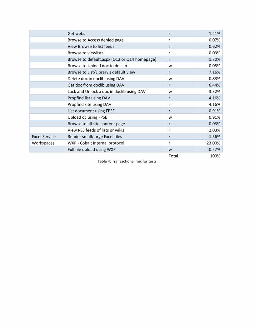
Get webs r 1.21%

Browse to Access denied page r 0.07%

View Browse to list feeds r 0.62%

Browse to viewlists r 0.03%

Browse to default.aspx (O12 or O14 homepage) r 1.70%

Browse to Upload doc to doc lib w 0.05%

Browse to List/Library's default view r 7.16%

Delete doc in doclib using DAV w 0.83%

Get doc from doclib using DAV r 6.44%

Lock and Unlock a doc in doclib using DAV w 3.32%

Propfind list using DAV r 4.16%

Propfind site using DAV r 4.16%

List document using FPSE r 0.91%

Upload oc using FPSE w 0.91%

Browse to all site content page r 0.03%

View RSS feeds of lists or wikis r 2.03%

Excel Service Render small/large Excel files r 1.56%

Workspaces WXP - Cobalt internal protocol r 23.00%

Full file upload using WXP w 0.57%

Total 100%

Table 4: Transactional mix for tests

Results and analysis

Test methodology We used Visual Studio Team System for Test 2008 SP2 to perform the performance testing. The testing

goal was to find the performance characteristic of green zone, max zone and various system stages in

between for each topology. Detailed definitions of “max zone” and “green zone” are given below in

terms of specific values of performance counters, but in general, a farm configuration performing

around “max zone” break point can be considered under stress, while a farm configuration performing

“green zone” break point can be considered healthy.

Max RPS criteria

o Throttling is on and no 503 errors

o Failure Rate is less than 0. 1%

o 75th percentile latency is less than 1 seconds

o SQL Server CPU <= 75% to account for Search crawls

o All front-end Web server CPUs <=75%

“Green Zone” criteria

o 75th percentile latency is less than 0.5 sec

o front-end Web server CPU is less than 50%

o SQL Server CPU is less than 40% (10% is to allow Search crawls)

o Application server CPU is less than 50%

o Failure rate is less than 0.01%

Note: To factor in the Search Crawl impact we modified the Green-zone definition to be 40% for SQL to allow 10% tax from Search crawls. Similarly, we used 75% SQL Server CPU as the criteria for max RPS. The test approach was to start with the most basic farm configuration and run a set of tests. The first

test is to gradually increase the load on the system and monitor its performance characteristic. From

this test we derived the throughput and latency at various user loads and also identified the system

bottleneck. Once we have this data, we identified at what user load did the farm exhibit green zone and

max zone characteristics. We ran separate tests at those pre-identified constant user loads for a longer

time. These tests ensured that the farm configuration is capable of providing constant green zone and

max zone performance at respective user loads, over longer period of time.

Later doing the test for the next configuration, we scale out the system to eliminate bottleneck

identified in previous run. We keep iterating this way until we hit SQL Server CPU bottleneck.

We started off with a minimal farm configuration of 1 front-end Web server /application server and 1

SQL Server. Through multiple iterations, we finally ended at 3 front-end Web servers, 1 application

server, 1 SQL Server farm configuration, where SQL Server CPU was maxed out. Below you will find a

quick summary and charts of tests we performed on each iteration to establish green zone and max

zone for that configuration. That is followed by comparison of green zone and max zone for different

iterations, from which we derive our recommendations.

The SharePoint Admin Toolkit team has built a tool called “Load Test Toolkit (LTK)” which is publically

available for customers to download and use.

Results from iterations (1 X 1, 1 X 1 X 1, 2 X 1 X 1, 3 X 1 X 1)

1 X 1 farm configuration

Summary of results

- On a 1 front-end Web server and 1 SQL Server farm, in addition to front-end Web server duties,

the same computer was also acting as application server. Clearly this computer (still called front-

end Web server) was the bottleneck. As presented in the data below, the front-end Web server

CPU reached around 86% utilization when the farm was subjected to user load of 125 users,

using transactional mix described earlier in this document. At that point, the farm exhibited max

RPS of 101.37.

- Even at a small user load, front-end Web server utilization was always very high to consider this

farm as a healthy farm. For the workload and dataset that we used for the test, this

configuration is not recommended as a real deployment.

- Going by definition of “green zone”, there isn’t really a “green zone” for this farm. It’s always

under stress, even at a small load. As for “max zone”, at the smallest load, where the farm was

in “max zone”, the RPS was 75.

- Since, front-end Web server was bottlenecked due to its dual role as an app server, for the next

iteration, we separated out app server on its own computer.

Performance counters and graphs

Various performance counters captured during testing 1 X 1 farm, at different steps in user load, are

presented below.

User Load 50 75 100 125

RPS 74.958 89.001 95.79 101.37

Latency 0.42 0.66 0.81 0.81

Front-end Web server CPU

79.6 80.1 89.9 86

Application server CPU

N/A N/A N/A N/A

SQL Server CPU 15.1 18.2 18.6 18.1

75th Percentile [sec] 0.3 0.35 0.55 0.59

95th Percentile [sec] 0.71 0.77 1.03 1

Table 5: Performance counters in a 1X1 farm configuration

Chart 1: RPS and Latency in 1 X 1 configuration

Chart 2: Performance counters in 1 X 1 configuration

1 X 1 X 1 farm configuration

0

0,1

0,2

0,3

0,4

0,5

0,6

0,7

0

20

40

60

80

100

120

50 75 100 125

RPS

75th PercentileLatency [sec]

0

20

40

60

80

100

120

50 75 100 125

RPS

WFE CPU

SQL CPU

Summary of results

- On a 1 front-end Web server, 1 application server and 1 SQL Server farm, front-end Web server

was the bottleneck. As presented in the data below, the front-end Web server CPU reached

around 85% utilization when the farm was subjected to user load of 150 users, using

transactional mix described earlier in this document. At that point, the farm exhibited max RPS

of 124.1.

- This configuration delivered “green zone” RPS of 99, with 75th percentile latency being 0.23 sec,

and the front-end Web server CPU hovering around 56 % utilization. This indicates that this farm

can healthily deliver an RPS of around 99. “Max zone” RPS delivered by this farm was 123 with

latencies of 0.25 sec and the front-end Web server CPU hovering around 85%.

- Since the front-end Web server CPU was the bottleneck in this iteration, we relived the

bottleneck by adding another the front-end Web server for the next iteration.


Various performance counters captured during testing 1 X 1 X 1 farm, at different steps in user load, are

presented below.

User Load 25 50 75 100 125 150

RPS 53.38 91.8 112.2 123.25 123.25 124.1


34.2 56 71.7 81.5 84.5 84.9


23.2 33.8 34.4 32 30.9 35.8

SQL Server CPU 12.9 19.7 24.1 25.2 23.8 40.9

75th Percentile latency [sec]

0.22 0.23 0.27 0.32 0.35 0.42

95th Percentile latency [sec]

0.54 0.52 0.68 0.71 0.74 0.88

Table 6: Performance Counters during 1 X 1 X 1 configuration

Chart 3: RPS and Latency in 1 X 1 X 1 configuration

Chart 4: Performance counters in 1 X 1 X 1 configuration


Summary of results

- On a 2 front-end Web server, 1 application server and 1 SQL Server farm, the front-end Web

server was the bottleneck. As presented in the data below, front-end Web server CPU reached

around 76% utilization when the farm was subjected to user load of 200 users, using

transactional mix described earlier in this document. At that point, the farm exhibited max RPS

of 318.

0

0,05

0,1

0,15

0,2

0,25

0,3

0,35

0,4

0,45

0

20

40

60

80

100

120

140

25 50 75 100 125 150

RPS

75th PercentileLatency [sec]

0

20

40

60

80

100

120

140

25 50 75 100 125 150

RPS

WFE CPU

APP CPU

SQL CPU

- This configuration delivered “green zone” RPS of 191, with 75th percentile latency being 0.37

sec, and front-end Web server CPU hovering around 47 % utilization. This indicates that this

farm can healthily deliver an RPS of around 191. “Max zone” RPS delivered by this farm was 291

with latencies of 0.5 sec and front-end Web server CPU hovering around 75%.

- Since front-end Web server CPU was the bottleneck in this iteration, we relived the bottleneck

by adding another front-end Web server for the next iteration.



presented below.

User Load 40 80 115 150 175 200

RPS 109 190 251 287 304 318

Latency 0.32 0.37 0.42 0.49 0.54 0.59


27.5 47.3 61.5 66.9 73.8 76.2


17.6 29.7 34.7 38 45 45.9

SQL Server CPU 109 190 251 287 304 318

75th Percentile [sec]

0.205 0.23 0.27 0.3 0.305 0.305


0.535 0.57 0.625 0.745 0.645 0.57

Table 7: Performance counters during 2X1X1 configuration

Chart 5: RPS and Latency in 2X1X1 configuration

0

0,05

0,1

0,15

0,2

0,25

0,3

0,35

0

50

100

150

200

250

300

350

40 80 115 150 175 200

RPS

75th PercentileLatency[sec]

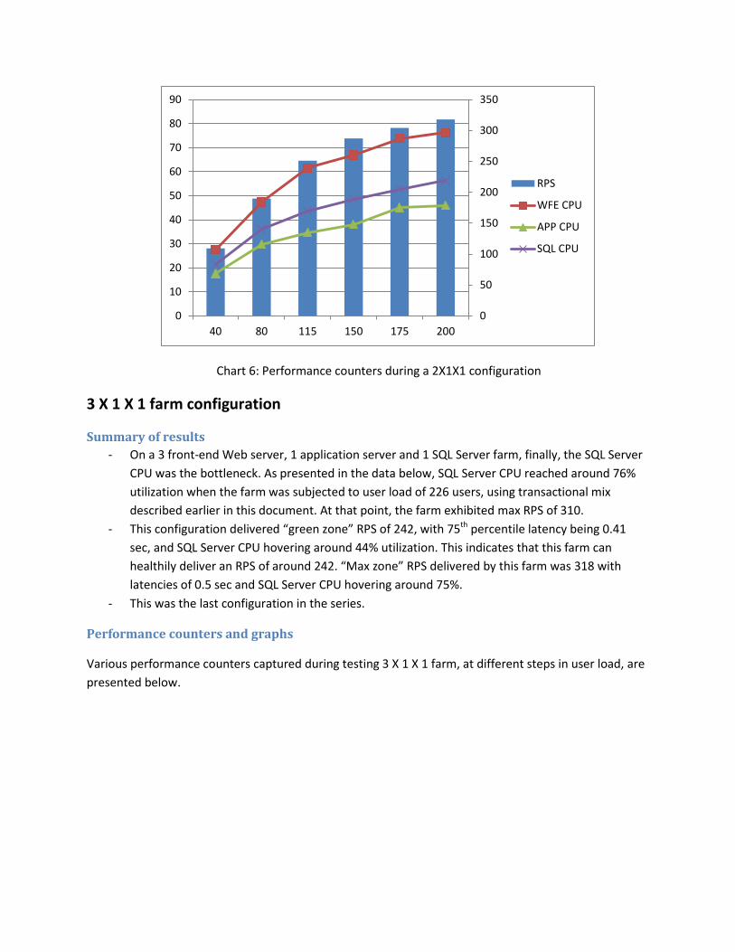
Chart 6: Performance counters during a 2X1X1 configuration


Summary of results

- On a 3 front-end Web server, 1 application server and 1 SQL Server farm, finally, the SQL Server

CPU was the bottleneck. As presented in the data below, SQL Server CPU reached around 76%

utilization when the farm was subjected to user load of 226 users, using transactional mix

described earlier in this document. At that point, the farm exhibited max RPS of 310.

- This configuration delivered “green zone” RPS of 242, with 75th percentile latency being 0.41

sec, and SQL Server CPU hovering around 44% utilization. This indicates that this farm can

healthily deliver an RPS of around 242. “Max zone” RPS delivered by this farm was 318 with

latencies of 0.5 sec and SQL Server CPU hovering around 75%.

- This was the last configuration in the series.



presented below.

0

50

100

150

200

250

300

350

0

10

20

30

40

50

60

70

80

90

40 80 115 150 175 200

RPS

WFE CPU

APP CPU

SQL CPU

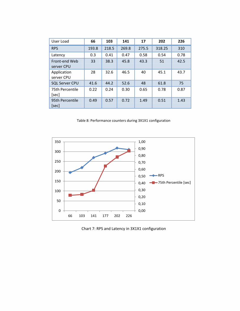
User Load 66 103 141 17 202 226

RPS 193.8 218.5 269.8 275.5 318.25 310

Latency 0.3 0.41 0.47 0.58 0.54 0.78


33 38.3 45.8 43.3 51 42.5


28 32.6 46.5 40 45.1 43.7

SQL Server CPU 41.6 44.2 52.6 48 61.8 75


0.22 0.24 0.30 0.65 0.78 0.87


0.49 0.57 0.72 1.49 0.51 1.43

Table 8: Performance counters during 3X1X1 configuration

Chart 7: RPS and Latency in 3X1X1 configuration

0,00

0,10

0,20

0,30

0,40

0,50

0,60

0,70

0,80

0,90

1,00

0

50

100

150

200

250

300

350

66 103 141 177 202 226

RPS


Chart 8: Performance counters during a 3X1X1 configuration

Comparison

From the step tests we performed, we found out the points at which a configuration enters max zone or

green zone. Here’s a table of those points.

The table and charts below provide a summary for all the results presented above.

Topology 1x1 1x1x1 2x1x1 3x1x1

Max RPS 75 123 291 318

Green Zone RPS n/a 99 191 242

Max Latency 0.29 0.25 0.5 0.5

Green Zone Latency 0.23 0.23 0.37 0.41

Table 10: Summary of results across different configurations

0

50

100

150

200

250

300

350

0

10

20

30

40

50

60

70

80

66 103 141 177 202 226

RPS

WFE CPU

APP CPU

SQL CPU

Chart 9: Summary of RPS at different configurations

Chart 10: Summary of Latency at different configurations

A note on disk I/O

Disk I/O based bottlenecks are not considered while prescribing recommendations in this

document, but it’s still interesting to observe the trend. Here are the numbers:

Configuration 1x1 1x1x1 2x1x1 3x1x1

Max RPS 75 154 291 318

Reads/Sec 38 34 54 58

Writes/Sec 135 115 230 270

Table 11: I/Ops across different configurations

0

50

100

150

200

250

300

350

1x1 1x1x1 2x1x1 3x1x1

Max RPS

Green Zone RPS

0

0,1

0,2

0,3

0,4

0,5

0,6

1x1 1x1x1 2x1x1 3x1x1

Max Latency

Green Zone Latency

Since we ran the tests in duration of 1 hour and the test exercises only a fixed set of sites/webs/doc libs

and so on , SQL Server could cache all the data. Thus, our testing caused very little Read IO. We see

more write I/O operations that read. It is important to note that this is an artifact of the test

methodology, and not a good representation of real deployments. Most of the typical divisional portals

would have more read operations 3 to 4 times more than write operations.

Chart 11: I/Ops at different RPS

Tests with Search incremental crawl

As we mentioned before, all the tests till now were run without Search crawl traffic. In order to provide

information on how ongoing search crawl can affect performance of a farm, we decided to find out max

end user RPS and corresponding end user latencies with search crawl traffic in the mix. We added a

separate front-end Web server to 3 X 1 X 1 farm, designated as a crawl target. We saw a 17% drop in

RPS as compared to original RPS exhibited by 3 X 1 X 1.

In a separate test, on the same farm, we used Resource Governor to limit available resources to search

crawl 10%. We saw that as Search utilizes lesser resources, max RPS of the farm climbs up by 6%.

These results are presented below.

Baseline 3X1X1

Only Incremental Crawl

No Resource Governor

10% Resource Governor

RPS 318 N/A 276 294.5

% RPS Difference from baseline 0% N/A 83% 88%

SQL Server CPU [%] 83.40 8.00 86.60 87.3

SA SQL Server CPU [%] 3.16 2.13 3.88 4.2

0

50

100

150

200

250

300

350

1x1 1x1x1 2x1x1 3x1x1

Max RPS

Reads/Sec

Writes/Sec

Front-end Web server CPU [%] 53.40 0.30 47.00 46.5

Application server CPU [%] 22.10 28.60 48.00 41.3

Crawl front-end Web server CPU [%] 0.50 16.50 15.00 12.1

Table 12: Results from tests with incremental Search crawl

Chart 12: Results from tests with incremental Search crawl

Important note

Here we are only talking about incremental crawl, on a farm where there aren’t very many changes to

the content. It is important to note that 10% resource utilization will be way too less for a full search

crawl. It may also prove to be less if there are way too many changes. It is certainly not advised to limit

resource utilization to 10% if you are running a full search crawl, or your farm generally sees a high

volume of content changes between crawls.

Summary of results and recommendations

To paraphrase the results from all configurations we tested:

With the configuration, dataset and test workload we had chosen for the tests, we could

scale to maximum 3 front-end Web servers before SQL Server was bottlenecked on CPU.

The absolute max RPS we could get at that point was somewhere around 318.

With each additional front-end Web server, increase in RPS was almost linear. We can

extrapolate that as long as SQL Server is not bottlenecked, you can add more front-end Web

servers and further increase in RPS is possible.

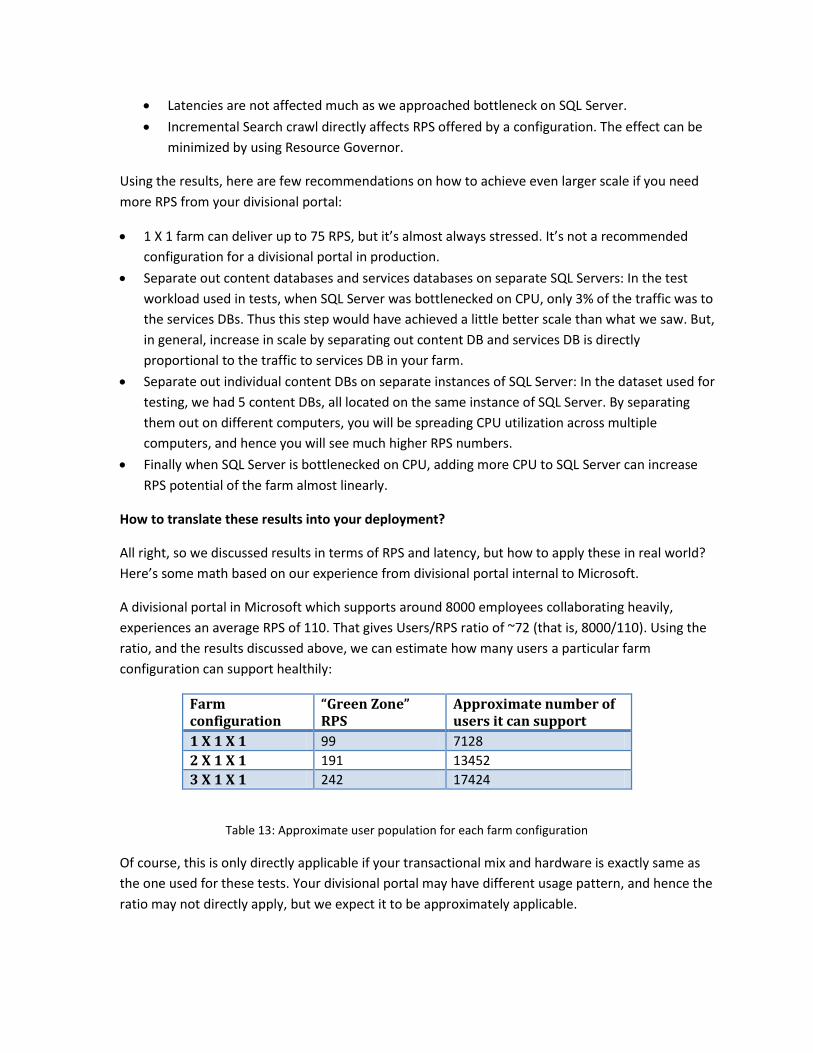
Latencies are not affected much as we approached bottleneck on SQL Server.

Incremental Search crawl directly affects RPS offered by a configuration. The effect can be

minimized by using Resource Governor.

Using the results, here are few recommendations on how to achieve even larger scale if you need

more RPS from your divisional portal:

1 X 1 farm can deliver up to 75 RPS, but it’s almost always stressed. It’s not a recommended

configuration for a divisional portal in production.

Separate out content databases and services databases on separate SQL Servers: In the test

workload used in tests, when SQL Server was bottlenecked on CPU, only 3% of the traffic was to

the services DBs. Thus this step would have achieved a little better scale than what we saw. But,

in general, increase in scale by separating out content DB and services DB is directly

proportional to the traffic to services DB in your farm.

Separate out individual content DBs on separate instances of SQL Server: In the dataset used for

testing, we had 5 content DBs, all located on the same instance of SQL Server. By separating

them out on different computers, you will be spreading CPU utilization across multiple

computers, and hence you will see much higher RPS numbers.

Finally when SQL Server is bottlenecked on CPU, adding more CPU to SQL Server can increase

RPS potential of the farm almost linearly.

How to translate these results into your deployment?

All right, so we discussed results in terms of RPS and latency, but how to apply these in real world?

Here’s some math based on our experience from divisional portal internal to Microsoft.

A divisional portal in Microsoft which supports around 8000 employees collaborating heavily,

experiences an average RPS of 110. That gives Users/RPS ratio of ~72 (that is, 8000/110). Using the

ratio, and the results discussed above, we can estimate how many users a particular farm

configuration can support healthily:

Farm configuration

“Green Zone” RPS

Approximate number of users it can support

1 X 1 X 1 99 7128

2 X 1 X 1 191 13452

3 X 1 X 1 242 17424

Table 13: Approximate user population for each farm configuration

Of course, this is only directly applicable if your transactional mix and hardware is exactly same as

the one used for these tests. Your divisional portal may have different usage pattern, and hence the

ratio may not directly apply, but we expect it to be approximately applicable.

capacity planning and sizing for microsoft sharepoint … planning and sizing for microsoft...

Documents