capacity scaling and spectral efficiency in wide-band

2504 IEEE TRANSACTIONS ON INFORMATION THEORY, VOL. 49, NO. 10, OCTOBER 2003

Capacity Scaling and Spectral Efficiency inWide-Band Correlated MIMO ChannelsKe Liu, Student Member, IEEE, Vasanthan Raghavan, Student Member, IEEE, and

Akbar M. Sayeed, Senior Member, IEEE

Abstract—The dramatic linear increase in ergodic capacitywith the number of antennas promised by multiple-input mul-tiple-output (MIMO) wireless communication systems is based onidealized channel models representing a rich scattering environ-ment. Is such scaling sustainable in realistic scattering scenarios?Existing physical models, although realistic, are intractable foraddressing this problem analytically due to their complicatednonlinear dependence on propagation path parameters, suchas the angles of arrival and delays. In this paper, we leverage arecently introduced virtual representationof physical models thatis essentially a Fourier series representation of wide-band MIMOchannels in terms of fixed virtual angles and delays. Motivatedby physical considerations, we propose a -connected model forcorrelated channels defined by a virtual spatial channel matrixconsisting of nonvanishing diagonals with independent andidentically distributed (i.i.d.) Gaussian entries. The parameter

provides a meaningful and tractable measure of the richnessof scattering. We derive general bounds for the coherent ergodiccapacity and investigate capacity scaling with the number ofantennas and bandwidth. In the large antenna regime, we showthat linear capacity scaling is possible if scales linearly withthe number of antennas. This, in turn, is possible if the number ofresolvable paths grows quadratically with the number of antennas.The capacity saturates for linear growth in the number of paths(fixed ). The ergodic capacity does not depend on frequencyselectivity of the channel in the wide-band case. Increasingbandwidth tightens the bounds and hastens the convergence ofscaling behavior. For large bandwidth, the capacity scales linearlywith the signal-to-noise ratio (SNR) as well. We also provide anexplicit characterization of the wide-band slope recently proposedby Verdú. Numerical results are presented to illustrate the keytheoretical results.

Index Terms—Beamforming, empirical eigenvalue distribution,ergodic capacity, Fourier series, frequency selectivity, ray tracing,scattering, spectral efficiency.

I. INTRODUCTION

T HE use of multiple-element antenna arrays has emergedas a promising technology for dramatically increasing

the spectral efficiency of wireless communication systems.Initial studies have indicated linear increase in the capacity of

Manuscript received November 1, 2002; revised June 22, 2003. This workwas supported in part by the National Science Foundation under CAREER GrantCCR-9875805 and ITR Grant CCR-0113385, and by the ONR under the YIPGrant N00014-01-1-0825. The material in this paper was presented in part atthe IEEE International Symposium on Information Theory, Yokohama, Japan,June/July 2003 and will be presented in part at the IEEE Global Communica-tions Conference, San Francisco, CA, December 2003.

The authors are with the Electrical and Computer Engineering Depart-ment, University of Wisconsin-Madison Madison, WI 53706 USA (e-mail:[email protected]; raghavan @cae.wisc.edu; [email protected]).

Communicated by B. Hassibi, Associate Editor for Communications.Digital Object Identifier 10.1109/TIT.2003.817446

narrow-band multiple-input multiple-output (MIMO) systemswith the number of antennas (see [1], [2]). However, thesestudies are based on an idealized channel model, representinga rich scattering environment, that assumes independent andidentically distributed (i.i.d.) Gaussian entries for the channelmatrix. Such idealized channels seldom, if ever, occur inpractice, particularly with practically feasible antenna spacings.Several experimental and analytical studies have shown thatthe capacity of realistic MIMO channels can be significantlyless than that of i.i.d. models (see [3]–[6]).

Idealized statistical models, such as those used in [1], [2],represent one extreme in existing modeling approaches. On theother extreme are detailed physical (ray-tracing) models that de-scribe the channel via signal propagation over multiple paths,each path associated with an angle of departure (AoD), an angleof arrival (AoA), a delay and a path gain (see, e.g., [7]–[9],[4], [10]). While quite accurate, such models depend on phys-ical AoAs, AoDs, and delays in a nonlinear fashion making itrather difficult to incorporate them in system design or analyt-ical calculations. Indeed, most capacity studies based on phys-ical models have relied on numerical simulation for capacity as-sessment (see, e.g., [4], [7], [8]).

The goal of this paper is to investigate capacity scaling in real-istic correlated MIMO channels. We consider both narrow-bandand wide-band channels and explore scaling behavior of ergodiccapacity as a function of both the number of antennas and band-width in a Rayleigh-fading environment. There are three mainobjectives of our work: 1) to provide a characterization of phys-ical MIMO channel models that is analytically tractable, 2) toobtain rigorous mathematical results that characterize capacityscaling behavior, and 3) to relate the scaling results to the phys-ical characteristics of realistic MIMO channels. Our focus is onsystems that use uniform linear arrays (ULAs) ofantennas atboth the transmitter and receiver. We assume that the channel isunknown at the transmitter but perfectly known at the receiver.

The workhorse of our analysis is a recently introducedvir-tual representationof narrow-band [6] and wide-band MIMOchannels [11], [12] that provides an intuitive and tractable char-acterization of realistic physical models and yields useful in-sights into the effects of scattering characteristics on channel ca-pacity. The virtual representation is based on the simple but fun-damental observation that detailed channel modeling without re-gard to signal space characteristics is unnecessary from a com-munication-theoretic viewpoint—aneffective channel represen-tationthat captures the interaction between the physical channeland the finite-dimensional space–time signal space is all thatis needed. In wide-band MIMO channels, the signal space is

0018-9448/03$17.00 © 2003 IEEE

LIU et al.: CAPACITY SCALING AND SPECTRAL EFFICIENCY IN WIDE-BAND CORRELATED MIMO CHANNELS 2505

characterized by the number of antennas(for a given an-tenna spacing) and bandwidth. The virtual representation isa Fourier series for the channel frequency response matrix thatcorresponds to sampling the angle-delay space atfixed virtualAoAs, AoDs, and delays. In particular, it induces a virtual par-titioning of propagation paths in angle-delay space that exposestheir contribution to channel capacity, and plays a key role inrelating the scaling results to physical scattering characteristics.

Our capacity scaling analysis is based on a-connectedmodel for the narrow-band virtual matrix that consists of

nonvanishing diagonals with i.i.d. Gaussian entries. The-connected model is motivated by physical considera-

tions—it represents a scattering environment in which eachvirtual transmit angle couples with virtual receive angles andvice versa. We call thechannel connectivityas it provides ameaningful and tractable measure of the richness of scattering.For example, corresponds to a loosely connected(highly correlated) channel, whereas represents a richscattering environment. In effect, the-connected model pro-vides a mathematical construct that greatly facilitates capacityanalysis of correlated channels, analogous to the role of i.i.d.channel matrix in the idealized model.

To our knowledge, the most recent work addressing the issueof capacity scaling in correlated channels is [13]. The channelmodel used in [13] is a generalization of the i.i.d. model and stillpredicts linear capacity growth with the number of antennas, al-beit with a smaller slope compared to i.i.d. channels. In SectionVII, we interpret the channel model in [13] in the context of ourframework. In particular, the results in this paper make a directconnection with physical models and precisely identify the sit-uations in which capacity scaling can or cannot occur.

Summary of Results:We investigate capacity scaling inboth the low-power and large antenna () regimes for bothnarrow-band and wide-band channels. Most of our analysisis based on general lower and upper bounds on the ergodiccapacity of the -connected model. First, consider thenarrow-band case. In the low-power regime, we show that

scales precisely as where denotes the capacity andthe total transmit power. The analysis in the large antenna

regime is greatly facilitated by a fortuitous connection betweenthe -connected model and some earlier work of Grenanderand Silverstein [14] on the limiting empirical eigenvaluedistribution of a class of random matrices. We show that forlarge , exhibits linear growth with if grows linearlywith as well. This, in turn, implies that linear capacitygrowth is sustainable in physical channels if the number ofresolvable paths grows quadratically with. For fixed ,which corresponds to linear growth in the number of paths, thecapacity saturates. For a finite number of paths, there is no gainin increasing beyond the number of paths.

In the wide-band case, we show that frequency selectivitydoes not affectergodiccapacity, which is consistent with knownresults in the single-antenna case [15]. In fact, wide-band ca-pacity is solely governed by spatial channel characteristics viaappropriate scaling with . The most conspicuous effect ofincreasing bandwidth is that it tightens the capacity boundsand hastens the convergence of scaling behavior. In particular,

for a large bandwidth, we get linear capacity growth withtransmit power as well. We also investigate spectral efficiencyof wide-band MIMO channels and provide explicit character-izations of the minimum energy per bit (required for reliablecommunication) and the wide-band slope recently proposed byVerdú [16].

The rest of this paper is organized as follows. In the next sec-tion, we present a general physical model for wide-band MIMOchannels, review the virtual representation and its relation to thephysical model. We also discuss channel statistics and virtualpath partitioning to motivate the-connected channel model. InSection III, we formally define the -connected model and ob-tain lower and upper bounds for its capacity. Section IV presentsour capacity scaling results for narrow-band MIMO channels.Section V contains a parallel set of results for wide-band chan-nels. Section VI investigates spectral efficiency issues. In Sec-tion VII, we provide a physical interpretation of the scaling re-sults and also provide illustrative numerical results. Section VIIIcloses the paper with concluding remarks. Several of the proofsare relegated to the Appendixes.

II. WIDE-BAND MIMO CHANNEL MODELING

In this section, we review the virtual representation for bothnarrow-band [6] and wide-band MIMO channels [11], [12] thatplays a key role in connecting the scaling results in this paperto the structure of physical MIMO channels. We focus on theaspects of the virtual representation that are particularly relevantto this paper. The reader is referred to [6], [11], [12] for details.Throughout this paper, we consider MIMO systems with ULAsof antennas at both the transmitter and receiver and assumethat far-field conditions apply.

A. A General Physical Model for Wide-Band MIMO Channels

We are interested in representing the MIMO channel over atwo-sided bandwidth . In the absence of noise, the transmittedand received signals are related as

(1)

(2)

where is the -dimensional transmitted signal in time,is the -dimensional received signal in time, and and

are Fourier transforms of and , respectively

(3)

The matrix represents theimpulse responsematrix and is the correspondingfrequency responsematrix (the Fourier transform of ) coupling thetransmitter and receiver elements. We will primarily workwith and we index the entries of as :

.1

1The subscript “c” denotes the actual channel matrix, as opposed to the virtualchannel matrix.


(a)

(b)

Fig. 1. A schematic illustratingphysical modelingversusvirtual represen-tation in the spatial dimension. (a)Physical Modeling: Each scattering path isassociated with a fading gain(� ) and a unique pair of transmit and receiveangles(� , � ). (b) Virtual Representationof the scattering environmentdepicted in (a). The virtual angles are fixeda priori and their spacing definesthe spatial resolution. The channel is characterized by the virtual coefficientsfH (q; p) = h g that couple theN virtual transmit anglesf' g withtheN virtual receive anglesf' g.

Let and denote the antenna spacings at the transmitterand receiver, respectively. The channel matrix for ULAs can bedescribed via the array steering and response vectors

(4)

where is related to the AoA/AoD variable (measured withrespect to the horizontal axis—see Fig. 1) as

, is the wavelength of propagation, and is thenormalized antenna spacing. We will primarily work with thespatial variable . We restrict ourselves to critical spacing:

. In this case, there is a one-to-one mappingbetween and . The effect oflarger antenna spacing on capacity and diversity is discussed indetail in [6].

The channel matrix can be generally modeled as

(5)

which corresponds to signal propagation along paths,where and represent the AoDs and AoAs, re-spectively, the delays, and the corresponding com-plex path gains. The physical model is illustrated in Fig. 1(a).

A narrow-band MIMO system corresponds to in whichcase (5) reduces to

(6)

Define

(7)

Then and represent theangular spreadsseen by the receiver and transmitter, respec-tively. Thedelay spreadis denoted by

(8)

Without loss of generality, we assume so that.

A continuous version of (5), corresponding to a continuum ofpropagation paths, is insightful in relating the channel matrix tothe scattering environment

(9)

where denotes theangle-delay spreading func-tion that characterizes the scattering environment. For the dis-crete model (5), it reduces to

(10)where denotes the Dirac delta function. For thenarrow-band case, (9) reduces to

(11)

(12)

where the second equality in (12) corresponds to the discretemodel (6).

B. A Virtual Representation for Wide-Band MIMO Channels

In (5), each propagation path is associated with an arbitraryAoD, AoA, and delay distributed within the angular and delayspreads. The virtual representation replaces the physical pathswith virtual ones corresponding tofixedAoDs, AoAs, and de-lays that are determined by the spatial and temporal resolution ofthe array. The notion of virtual angles is illustrated in Fig. 1(b).Without loss of generality, assume that is odd and define

.


Definition 1—Virtual Channel Representation:The virtualchannel representation is defined by the Fourier series expan-sion [6], [11], [12]

(13)

corresponding tofixed virtualAoDs, AoAs, and delays

(14)

The virtual (Fourier series) channel coefficientscharacterize the virtual representation and can be computedfrom as

(15)

Combining (15) and (9) we get

(16)

where the second equality corresponds to the discrete model and

(17)

(18)

Note that and get peaky around the origin withincreasing and . Thus, (16) states that the virtual channelcoefficients are samples of a smoothed version of the delay-angle spreading function, and that the smoothing kernel getsnarrower with increasing and .

The spacing between the transmit/receive virtual angles in(14) represents the spatial resolution of the array:

. Similarly, the spacing between the virtual delayscorresponds to the temporal resolution: . Forsufficiently large and , most of the channel power iscarried by a subset of the coefficients. The size of this subset ofdominant is determined by the angular and delayspreads [6], [11], [12]

(19)

(20)

(21)

In the narrow-band case, virtual representation reduces to

(22)

(23)

where and are discrete Fourier transform (DFT)(unitary) matrices. The elements of the narrow-band virtual ma-trix are related to the discrete physical model as

(24)

We note that the virtual representation is a unitary transforma-tion of the actual channel matrix and, thus, all capacity-relatedissues can be equivalently investigated in the virtual domain.

C. Virtual Path Partitioning

The virtual representation induces a partitioning of paths thatis very insightful in relating physical scattering characteristicsto channel statistics.

Definition 2—Virtual Path Partitioning:Define the fol-lowing subsets of propagation paths:

(25)

(26)

(27)

corresponding to the spatial and delay resolutions. The abovesets form a partition

(28)

(29)

With the path partitioning, the virtual coefficients in (16) and(24) can be approximated as

(30)

where and .Thus, in the narrow-band case, the paths are distributed in thevirtual representation according to the spatial resolution. In thewide-band case, this distribution is further refined by the delayresolution.

D. Statistics of Wide-Band Correlated MIMO Channels

In this paper, we are interested in modeling the channel overtime scales over which the locations of scatterers, and hence


, , and , do not change significantly relativeto the transmitter and receiver. This is equivalent to consideringtime scales over which the channelstatisticsdo not change ap-preciably. However, the channel realizations do vary over suchtime scales due to the phase variations in path gains.

We make the following (Rayleigh fading) assumption onphysical scattering.

Assumption 1—Independent Physical Scattering:The phys-ical channel parameters , , and are fixedover the time scales of interest. The path gains are inde-pendent zero-mean complex circular Gaussian random variableswith variances

(31)

where denotes the Kronecker delta function.Under the above assumption, the elements of are

jointly complex circular Gaussian, and, consequently, so are thevirtual coefficients . Assumption 1 implies uncor-related statistics for the spreading function in (10) [6], [11]

(32)

(33)

The nonnegative function in (32) is called theangle-delay scattering function(or angle-delay power profile)and reflects the distribution of channel power in thespace; it is given by (33) for the discrete model.

An important property of the virtual representation is thatare approximately uncorrelated (and, hence, ap-

proximately independent) under Assumption 1 [6], [11], [12]

(34)

(35)

(36)

and (using (4), (5), (13))

(37)

(38)

Equations (38) and (34) state that the elements of forma three-dimensional stationary random field and the virtual co-efficients are samples of a smoothed version of itsunderlying spectral representation and are hence approximatelyuncorrelated. The scattering function can be in-terpreted as the power spectral density2 associated with ,and the dominant virtual coefficients

approximately characterize theindependent degrees of freedomin wide-band MIMO channels.

The following observation will be useful in wide-band ca-pacity results.

Proposition 1: At any given frequency, the spatial statisticsof are independent of.

Proof: The proof directly follows from (38) by substi-tuting .

Thus, thespatial statistics of are determined by thestatistics of the narrow-band matrix (or, equiva-lently, ). The total channel power is distributed as[11], [12]

(39)

E. -Diagonal Virtual Model for Narrow-Band MIMOChannels

We now motivate a simple model—the-diagonal virtualmodel—for correlated narrow-band MIMO channels that playsa key role in the scaling results. As we will see, the ergodic ca-pacity of wide-band MIMO channels depends only on spatialstatistics of the narrow-band virtual matrix. Spectral statisticsonly contribute to diversity and hence affect the outage capacity[11], [12].

Consider a single scattering cluster with maximum an-gular spreads at the transmitter and receiver:

. One source of correlation is limited angularspreads. However, the effective angular spread (in thedo-main) can be maximized (and the channel decorrelated) in suchcases by increasing the antenna spacing [6]. For maximumangular spreads, the nature of coupling between the scattererswithin the cluster determines the channel correlation. On oneextreme is “diagonal scattering” ( diagonal), in which eachvirtual transmit angle couples with only a single correspondingvirtual receive angle. This corresponds to a scattering environ-ment consisting of a single line of scatterers (see [6, Fig. 7(a)]).In this case, is nonzero only for and the channelexhibits significant correlation since only out of degreesof freedom are excited. On the other extreme is “maximallyrich scattering” (all elements of nonzero) in which eachvirtual transmit angle couples with all virtual receive angles,

2The angular spreads represent the bandwidths associated with the stationaryfield in the spatial dimensions.


(a)

(b)

Fig. 2. A schematic illustrating thed-diagonal and circulantd-diagonalmodels for the virtual spatial matrix.N = 9 and d = 2 and each smallsquare represents a spatial resolution bin of size�� = �� = 1=N . (a)d-diagonal model consisting ofd nonvanishing diagonals above and below themain diagonal. Notice the truncation near the corners. (b) Circulantd-diagonalmodel. The truncated parts in (a) are wrapped around (aliased) and includedin the matrix as the dark grey circles.

andvice versa. This corresponds to multiple lines of scatterers(see [6, Fig. 7(b)]) and the channel will exhibit minimal cor-relation since all are nonzero. In particular,corresponds to the i.i.d. model. Thus, we can capture a richclass of scattering environments, depicting varying levels ofcorrelation, by imposing the following-diagonal structure on

:

for (40)

nonzero for

otherwise

(41)

where represents the number of nonvanishingdiagonals above and below the main diagonal (see Fig. 2(a)).Diagonal scattering corresponds to and maximally richscattering corresponds to .

The scaling results presented in subsequent sections are basedon a -connectedmodel which corresponds to the followingcirculant definition of -diagonal model:

for (42)nonzero for ,

where

otherwise.

(43)

The circulant modification is made for a technical reason—tomake the number of nonvanishing elements in each column andeach row to be the same—and does not affect the essential con-clusions of our results. It can be shown that thecirculant struc-ture in (43) actually occurs in systems which employ larger than

antenna spacing due to notion ofspatial aliasing[6].3 Thedifference between-diagonal and circulant-diagonal modelsis illustrated in Fig. 2. For the-diagonal model in Fig. 2(a),notice the truncation near the corners of the matrix. In the cir-culant -diagonal model in Fig. 2(b), the truncated parts in Fig.2(a) are wrapped around (aliased) and included in the matrix asdepicted by the dark grey circles.4

We assumed to be odd in the above discussion. We willrelax this assumption in the following sections. Furthermore,in the -connected model introduced in Section III, corre-sponds to the total number of diagonals; for oddand for even.

1) Alternative Interpretations for the -Connected Model:Let denote the joint density of path angles; the

angular spreads correspond to supports of the marginal den-sities. Consider maximum angular spreads:

. The path angles can be thoughtof as drawn independently according to . The -con-nected model corresponds to the following structure on the con-ditional density of given :

nonzero if

otherwise

(44)

where . Thus, even though the marginalsand span the entire angular spreads, the conditional den-sity exhibits a limited spread; .Note that is a normalized version of power spectraldensity

and may be estimated in practice from measurements (see, e.g.,[4]). Finally, since the sampling resolution is ,

in (44).

3For larger than�=2 antenna spacing, the principal� range([�1=2; 1=2])maps into a subset of the physical angle� range([��=2; �=2]) (e.g., the blackdots in Fig. 2(b)). However, due to the periodicity of steering and response vec-tors in�, scatterers outside the limited� range wrap into the principal� range(the grey dots in Fig. 2(b)). This is the notion of spatial aliasing.

4Note that only two light-grey colored truncated parts are included in the cir-culantd-diagonal matrix. In general, all four truncated parts may be aliased toyield the dark-grey parts. This would result in the dark-grey parts having twiceas much power as the black parts. However, such a situation is less likely inpractice and is not critical to the essence of our scaling results. Thus, this tech-nical point is ignored in the definition of theD-connected model.


Fig. 3. Plot ofN =N as a function ofN for p = 0:99.

2) Number of Paths Needed to Populate a-ConnectedChannel: For given and , a natural question (that willbe useful later) is: how many propagation paths are needed topopulate a -connected channel? The relation (30) states thatwe need at least as many paths as the number of nonvanishingentries, (see Fig. 2(b)), in the -connected model.This applies toresolvable pathsthat lie in distinct virtual spatialbins of size , as depicted in Fig. 2.However, since the path angles are randomly distributed, morethan paths will be needed to ensure with high probabilitythat there is at least one path in each spatial bin. Assume that

are uniformly distributed over theregion in (44). Then, each path can land, with equal probability,in any of the spatial bins and it can be shown that theprobability that the -connected model is fully populatedsatisfies

(45)

Fig. 3 plots the values of as a function of for. Even though , it is

evident that is bounded by a constant on the orderof for values of of interest. Thus, we conclude thatthe number of paths needed to populate a-connected channelwith high probability satisfies

(46)

III. -CONNECTEDCHANNEL MODEL AND CAPACITY BOUNDS

In the following, we focus on narrow-band systems and im-pose a spatial structure on correlated MIMO channels via thevirtual representation. The channel equation at any time instantcan be written equivalently in thevirtual domain as

(47)

where , , and are the -dimensional transmitted signalvector, receive signal vector, and complex Gaussian noisevector, respectively. The noise vector is assumed to be whitein space as well as over time. We assume thatis zero-meancomplex Gaussian with unit variance entries. The entries ofthe narrow-band virtual matrix are uncorrelatedzero-mean complex Gaussian random variables whose variancemay vary depending on the physical environment. In particular,many entries may be zero if the scattering is not rich enough tocouple all the transmit and receive dimensions.

A concise way to describe such a pattern inis via the notionof the Hadamard product. Let and be

matrices. The entries of the Hadamard product (writtenas ) are given by

(48)

Let where is the variance of the th entry in. The virtual channel matrix can then be expressed as

(49)


where consists of i.i.d. standard complex Gaussian randomvariables. Therefore, one can describe channel structure byspecifying , which we call thechannel pattern mask. Weassume that the nonvanishing elements ofhave identicalvariance.

Definition 3: A -connected channel with dimension,, is an MIMO channel whose channel

pattern mask is given by

if

whereif is odd

if is evenotherwise.

(50)

Note that the pattern mask matrix of-connected channelsis acirculant matrix with equal number of nonzero (unit)entries in each row and each column. The parameteris calledthe channel connectivity. It models the degree of coupling be-tween transmit–receive antenna pairs. When , the antennaarray is loosely coupled (strongly correlated), whilerepresents a densely coupled rich scattering environment (com-pletely uncorrelated). Fig. 4 illustrates a-connected channel ofdimension . Its channel pattern mask is given by

Proposition 2: Let be the channel matrix of a -con-nected channel of dimension. Then

(51)

Proof: It trivially follows from the definition of -con-nected channels.

The channel connectivity has a significant effect on thestatistics of . The special case of -connected channel when

precisely gives rise to the commonly used i.i.d. channelmodel. As pointed out in [2], [17], in this case isisotrop-ically distributed, that is, and have the same distribu-tion for any unitary matrix . The exploitation of the isotropicproperty of i.i.d. has been the key to many elegant resultsregarding capacity and coding for i.i.d. channels (see, e.g., [2],[17]). However, if , is no longer isotropically dis-tributed. In other words, isotropic property ofis rather a rarityin correlated channels, such as-connected channels. However,a weaker form of channel statistics turns out to be preserved as

scales. The following lemma connects the statistics of-con-nected channels to a (scaled) doubly stochastic matrix (DSM),which plays a role analogous to that of the isotropic distributionin i.i.d. channels.

Lemma 1—Scaled Doubly Stochastic Matrix:Let repre-sent a -connected channel. For an arbitrary unitary matrix,

Fig. 4. A schematic illustratingD-connected channels. The dimension is5

and the connectivity is3. Observe each transmit dimension is coupled with threereceive dimensions andvice versa.

denote and . Then, is a scaleddoubly stochastic matrix with scale, that is,

(52)

(53)

Proof: Since is a unitary matrix, (52) holds by noticing

(54)

The verification of (53) requires the circular property of the-connected channel. For given

(55)

where is the th entry in and is the set of columnindexes of corresponding to nonzero entries in theth rowof the channel pattern mask matrix. Note that the-connectedchannel structure implies that every row index of theth columnof is covered exactly times, and hence the above sum isequal to , which proves the lemma.

Assuming perfect knowledge of at the receiver, the ergodiccapacity of an Gaussian MIMO channel is given by [2]

(nats/s) (56)

where the maximization is over a set of positive semidefiniteHermitian matrices satisfying the power constraint ,and the expectation is with respect to random channel matrix.In the following, the base is implicitly assumed for unlessspecified otherwise.

An obstacle in analyzing capacity of realistic MIMO channelsis the optimal input distribution in (56). Except for diagonalchannels , i.i.d. channels , and a few othercorrelated cases [18]–[20], the optimal is unknown, whichlimits the strength of capacity results for these channels. The


doubly stochastic structure in Lemma 1 greatly facilitates ca-pacity analysis of -connected channels. The following upperbound plays a vital role in our capacity analysis of-connectedchannels. Although it can be alternatively proved by exploitingthe DSM property (Lemma 1) as in Appendix I, we present asimpler proof.5

Lemma 2—General Upper Bound:The capacity of a -con-nected channel of dimension is upper-bounded by

(57)

where is the total transmit power.Proof: The key is the fact that

for an positive semidefinite matrix , which is a dis-guised form of geometric meanarithmetic mean. The lemmais proved by the following chain of inequalities:

(58)

We next give two lower bounds for capacity of-connectedchannels. The first (Lemma 3) follows from a quick observa-tion that channel capacity is lower-bounded by the mutual in-formation corresponding to the uniform power input distribu-tion, that is, in (56). The key to the second(Lemma 4) is to construct a suboptimal channel from the orig-inal MIMO channel and then to evaluate the capacity of thesuboptimal channel, thus obtaining a looser but more tractablelower bound.

Lemma 3—Uniform Power Lower Bound:Given totaltransmit power , the capacity of a -connected channel ofdimension is lower-bounded by

(59)

where is the total transmit power.

Lemma 4—Rayleigh Subchannel Lower Bound:Given totaltransmit power , the capacity of a -connected channel ofdimension is lower-bounded by

(60)

where is a unit variance chi-square random variable with twodegrees of freedom.

Proof: See Appendix II.

5Thanks to the input of an anonymous reviewer.

IV. CAPACITY SCALING IN NARROW-BAND CHANNELS

A. Finite Connectivity

We first study capacity saturation and scaling behavior whenthe channel connectivity is finite.

1) Large-Dimensional Asymptotics:

Theorem 1—Capacity Saturation:Channel capacity of anMIMO channel with fixed connectivity at a given

transmit power is asymptotically bounded between andas approaches infinity.6

Proof: We write to emphasize capacity as a func-tion of array dimension. The upper bound is an immediate corol-lary of the general upper bound lemma (Lemma 2) since

as (61)

In view of Lemma 4, channel capacity is lower-bounded by

(62)

where is a unit variance chi-square random variable with twodegrees of freedom. Note

pointwise

Since

by and , the dominatedconvergence theorem (DCT) [21] implies that

(63)

Therefore,

(64)

which completes the proof.

2) Low-Power Regime:We write to emphasize ca-pacity as a function of transmit power.

Theorem 2—Capacity Scaling:For fixed and, the capacity of a -connected channel scales like

as becomes small. More precisely

(65)

Moreover, any Gaussian input satisfying achievescapacity asymptotically in the low-power regime. In particular,uniform power distribution, i.e., is asymptotically op-timal.

6A seriesfx g is said to be asymptotically bounded betweenA andB iffA � lim inf x � lim sup x � B.


Proof: Again, an application of the general upper boundreads

(66)

For the other direction, denote by for the un-ordered eigenvalues of , where is the input powerdistribution satisfying the power constraint. The unorderedeigenvalues are obtained by random permutation of all eigen-values of . Note that all unordered eigenvalues havethe same marginal distribution. It follows from

and that . Let denote themutual information corresponding to power. Similar to theproof of Theorem 1, the DCT can justify passing the limit in thefollowing:

(67)

B. Infinite Connectivity

A particularly interesting scenario is when the scattering en-vironment is rich enough to sustain a growth in channel connec-tivity with antenna dimension. We study the asymptotic (large

) capacity scaling behavior in such infinite connectivity envi-ronments.

1) Empirical Spectral Distribution of Large-DimensionalRandom Matrices:The essential mathematical tool we will beusing in studying the infinite connectivity case is the so-calledspectral analysis of random matrices. Interested readers arereferred to [22] for an excellent review on this subject. Inthe following, we make a brief introduction and clarify somecommon misconceptions in applying the random matrix theory.

Definition 4: Let be an Hermitian matrix and de-note by its eigenvalues. Theempirical spectraldistribution (ESD) of is defined by

(68)

where denotes the number of elements in the set indicated.

Note that itself is arandomvariable as it depends on out-comes of random matrix . A common practice is to regardsimply as the distribution of eigenvalues of. In most applica-tions, the quantities in interest, such as channel capacity, can beexpressed as

(69)

where the expectation is with respect to random matrixofdimension . For some type of random matrices, their ESDstend to converge in a certain sense as the dimension gets large.A prevailing practice in engineering is to treat as conver-gent. However, the next theorem demonstrates the crucial differ-ence between ESD and distribution of eigenvalues, which sets arigorous ground for our channel capacity investigation.

Theorem 3: Let be as in (69). Assume the set of non-negative functions is equicontinuous[23], that is, if

for every , there is a neighborhood of such thatfor all and all . Suppose that

converges to pointwise and that the ESDs convergepointwise as to a deterministic almost surely,written as a.s. Then

(70)

Proof: See Appendix III

2) Large Dimension Asymptotics:Consider a series of -connected channels with increasing dimension . Westudy its capacity behavior when channel connectivity growsproperly with . More precisely

and (71)

where we write to emphasize the dependency of connec-tivity on dimension and is called thegrowth ratioof connec-tivity.

A similar model has been considered in [14] when partiallyconnected neural networks exhibitlimiting ESD (LESD). Al-though the random network in [14] consists of -valuedrandom variables, its adaptation to our case is essentiallystraightforward. We state the following theorem and relegateits proof to Appendix IV.

Theorem 4—Grenander and Silverstein’77:Assumeas . Let be the ESD of .

Then, converges pointwise in probability to

for

for

for

(72)

where

(73)

is the so-called Marcenko–Pastur law.

The ESDs of random -connected channel matrices areshown in Fig. 5. As seen from the figure, the ESDs forare quite close to the limiting Marcenko–Pastur law.

With the aid of the above results, we come to the main the-orem of this section.

Theorem 5—Normalized Capacity Scaling:For fixed trans-mit power , if the channel connectivity grows properly withdimension , that is, (71) is satisfied, then the capacity per di-mension is asymptotically bounded as

(74)

where is the Marcenko–Pastur law given in (72) andisthe growth ratio.

Proof: Applying Jensen’s inequality and carrying out in-tegration, one can verify, indeed, that


Fig. 5. The empirical spectral distributions of randomD-connected channel matrices. The growth ratio is = 0:5. The Marcenko–Pastur law is also plotted.

The upper bound in (74) is again obtained from Lemma 2 bynoting that

We resort to Theorem 3 for the lower bound. The key is to eval-uate the mutual information for uniform power input. One has

(75)

where ’s are the unordered eigenvalues of andis the corresponding ESD. For

(76)

for some . Since

(77)and, hence, are equicontinuous. Also, foreach

In Theorem 4, the convergence of ESD is only in probability.However, there exists a subsequence such that thecorresponding ESD converges almost surely [21]. For the inves-tigation on capacity of a large antenna array, this seems to poseno serious constraint. So, we neglect this difficulty here.7 Then,it follows from Theorem 3 that

(78)

Thus, the proof is complete.

Fig. 6 shows plots of normalized capacity (upper and lowerbounds) as a function of for . The asymptotic limitsof the bounds are also plotted. It can be seen that the “capacity”corresponding to the uniform power distribution (lower bound)seems to converge exactly to the lower limit calculated from theMarcenko–Pastur law. We would like to leave it as a conjecturealthough we have shown a weaker result in Theorem 5.

V. CAPACITY SCALING IN WIDE-BAND MIMO CHANNELS

In this section, we discuss the ergodic capacity of the wide-band MIMO channel characterized by the transfer functionmatrix in the virtual spatial domain. Assuming perfectknowledge of at the receiver, the ergodic capacity of thewide-band channel is given by

(79)

7It seems from [22] that the convergence is almost surely.


Fig. 6. Normalized narrow-band capacityC(N)=N as a function ofN in an infinite connectivity channel. The growth ratio = 0:5 andP = 20 dB.

where the maximization is over a family of input Gaussian co-variance matrices that satisfy thetotal power constraint

(80)

The above definition of wide-band ergodic capacity is consistentwith that obtained in [24] for single-antenna frequency selectiveadditive white Gaussian noise (AWGN) channels.

Since the integrand in (79) in nonnegative, finding the optimalfamily is equivalent to finding the optimal at each

. Furthermore, at any, the optimal only depends on thespatial statistics of . From Proposition 1, we know that thespatial statistics of are independent of. Thus, the same

is optimal for all and the expression (79) for wide-bandergodic capacity reduces to

(81)

where denotes the narrow-band MIMO channelmatrix and . Since the wide-band ergodic ca-pacity does not depend on channel correlation over frequency,we immediately have the following result.

Theorem 6: Frequency selectivity does not affect the ergodiccapacity of wide-band MIMO channels.

Thus, whether we have a small or large delay spread doesnot affect the ergodic capacity, just as in the single-antenna case[15]. Note that some recent results suggested otherwise [25].However, a correct interpretation of the results in [25] is consis-

tent with Theorem 6.8 Recent experimental measurements sup-port the conclusions of Theorem 6 as well.

Remark 1: Note that (81) is identical to the expression fornarrow-band capacity (56) except for the linear capacity scalingdue to bandwidth and the replacement ofby . Withthe above connection between narrow-band and wide-bandcapacity, most of the narrow-band results directly carry over.In particular, the -connected model for the narrow-bandMIMO channel can be used in the wide-band case as well sincethe ergodic capacity is governed by spatial statistics of thenarrow-band matrix . Thus, in all the following results, weassume a -connected spatial structure for.

Theorem 7—General Wide-Band Capacity Bounds:For anyfixed and , the wide-band ergodic capacity can be boundedas

(82)

Proof: The result directly follows from Lemmas 2 and 3.

From Lemma 4, we also have the following looser but moretractable lower bound for :

(83)

8The numerical results in [25] show an increase in ergodic capacity with in-creased delay spread. However, under the modeling assumptions in [25], an in-crease in delay spread is associated with a corresponding increase in angularspread. Thus, the increase in capacity is actually due to the increase in angularspread, which is a well-understood effect (see, e.g., [6]). If the delay spread ischanged, while keeping the angular spread constant, there is no change in er-godic capacity [11], [12], as in Theorem 6.


Note that both the lower and upper bounds above increasewith .

A. Finite Connectivity Channels

Theorem 1 holds true for the wide-band channel as well.

Theorem 8—Asymptotic Wide-Band Capacity for FinitelyConnected Channels:Channel capacity of anwide-band MIMO channel with fixed connectivity at a giventransmit power is asymptotically bounded between and

as approaches infinity.

Theorem 2 for the low-power regime also carries over un-changed.

Theorem 9—Wide-Band Capacity Scaling in the Low-PowerRegime: For fixed , , and , the capacity ofa -connected wide-band channel scales like as becomessmall. More precisely

(84)

Moreover, any Gaussian input which satisfies the powerconstraint achieves capacity asymptotically in the low-powerregime. In particular, is asymptotically optimal.

B. Infinite Connectivity Channels

The capacity scaling result (Theorem 5) for infinitely con-nected narrow-band channels also carries over, except for ap-propriate bandwidth scaling.

Theorem 10—Normalized Wide-Band Capacity Scaling:Forfixed transmit power and bandwidth , if the spatial channelconnectivity grows properly with dimension, that is, (71) issatisfied, then the wide-band capacity per spatial dimension isasymptotically bounded as

(85)

where is the Marcenko–Pastur law given in (72) andisthe growth ratio.

C. Infinite Bandwidth Channels

It can be shown that as increases, both the lower and upperbounds in Theorem 7 converge to the same limit. The proof issimilar to the more direct proof provided below.

Theorem 11—Infinite Bandwidth Capacity:For any givenand transmit power , the infinite bandwidth capacity of a

-connected MIMO channel is equal to

(86)

Consequently, any Gaussian input satisfying the power con-straint achieves capacity.

Proof: It follows from (81) that

(87)

Now we have

(88)

where are the eigenvalues of . By DCT we have

(89)

where the last equality follows from Proposition 2. Combining(87) and (89) completes the proof.

If scales linearly with then the infinite bandwidthcapacity also scales linearly with . Moreover, in the infinitebandwidth case, the capacity also scales linearly with thetransmit power or the signal-to-noise ratio (SNR). The mostconspicuous effect of large bandwidth is that capacity ap-proaches the upper bound in the finite connectivity case and theupper and lower bounds converge in the infinite connectivitycase.

Fig. 7 shows the upper and lower bounds for as afunction of for and . We note that both boundsincrease with and are converging to as pre-dicted by Theorem 11. We have also plotted the largeboundsfor for comparison. It is worth noting that the plots forlarge are nearly identical to those for , demonstratingthe relatively fast convergence with.

VI. SPECTRALEFFICIENCY IN WIDE-BAND MIMO CHANNELS

The tradeoff of spectral efficiency versus energy per infor-mation bit is the key measure of channel capacity in wide-bandMIMO channels. Following [16], we investigate such a funda-mental tradeoff for correlated MIMO channel via the virtualchannel representation. Our results reveal an intrinsic linkbetween channel structure and characteristics of the band-width–power tradeoff. We shall begin with an exposition that istailored to our setup. Readers should consult the original work[16] for an elaborated treatment of spectral efficiency in thewide-band regime.

The wide-bandadditive white Gaussian noise(AWGN)channel is perhaps the best example to illustrate the tradeoff ofspectral efficiency and energy per information bit. The capacityof wide-band AWGN with bandwidth (Hz) is given by

(90)

where noise is assumed to have unit variance andis the totaltransmit power. Denote by the energy per dimension(J/s/Hz). Normalized by total bandwidth, the spectral efficiencyor capacity per dimension (b/s/Hz) is

(91)


Fig. 7. Normalized wide-band capacityC (N)=N as a function of bandwidth.N = 6, D = 3, P = 20 dB. The largeN limits correspond to =D(N)=N = 0:5.

Since the energy required to supportbits is per dimension,the energy per information bit (J/b) is simply given by

(92)

As the bandwidth approaches infinity or, equivalently, asthe energy per dimension approaches , spectral efficiencyconverges to. However, the infinite bandwidth capacity is pos-itive and

1.59 dB (93)

which is theminimum energy per information bitrequired forreliable communication [16].

Generally, let be the Shannon capacity per dimensionwhere is the energy per dimension. The spectral efficiencyversus energy per information bit (– ) tradeoff is a curve pa-rameterized by the energy per dimension (see [16, eqs.(15) and (16)]) as

(b/s/Hz) (94)

(dB-J/b) (95)

The region of – curve near is of great interest forwide-band applications. Asapproaches zero, converges tothe minimum energy per information bit required forreliable communications. Although spectral efficiency dimin-ishes as bandwidth increases, its decay near , that is, theslope of – at , is a key measure in assessing systemcapacity in the wide-band regime. The explicit parameterization

of the tradeoff curve with respect tois quite convenient to com-pute and .

Theorem 12—See [16]:Assume and exist on aneighborhood of .9 Then

(96)

(97)

Proof: We provide a proof based on (94) and (95). ApplyL’Hospital’s rule to get (96) as

Note that

(98)

Now applying L’Hospital’s rule repeatedly on (94) and (95), onehas

which is (97).

9Note that the units ofC(s) are in bits per dimension (as opposed to nats perdimension) which results in a constant offset compared with the correspondingformula in [16].


We next characterize the fundamental– tradeoff inwide-band MIMO channels. We shall adopt the practice ofnormalizing capacity by antenna dimensions as in [16], that is,the capacity unit is b/s/Hz/antenna, and correspondingly theenergy per dimension is given by

(99)

where is the total transmit power, is the antenna dimension,and is the bandwidth. Since it is hard to find the optimal inputdistribution in general, we use the capacity bounds.

Theorem 13—Minimum Energy Per Information Bit:Givena wide-band -connected channel of dimension, then

dB (100)

Proof: It follows from Theorem 7 that

(101)

where is an unordered eigenvalue of with .Trivially

Similar to the proof of Theorem 2, the DCT can justify the fol-lowing:

Then, (100) results from taking on both sides of

The wide-band slope concerns local behavior of–tradeoff for small values of energy per dimension. To facil-itate exposition, we normalize the input (Gaussian) distribution.

Definition 5—Normalized Input Distributions:Let be theset of all semipositive-definite Hermitian matrices corre-sponding to the covariance matrices of-dimensional complexGaussian input distributions. Given any , write

(102)

where , that is, write any as a product of a scalar anda normalizedpositive-definite Hermitian matrix whose trace isfixed at . Denote by the set of such matrices. Note thatany has a fixed trace equal to .

Using the notion of normalized input distributions, we canwrite the the power constraint as

(103)

where is the total transmit power. Then, the channel capacityformula can be rewritten as

(104)

where the maximization is over all normalized input distribu-tions and is the unordered eigenvalue of . Therefore,the optimal – tradeoff curve is given by (94) and (95) with

(105)

The proof of Theorem 13 shows that uniform power distribu-tion, that is, , asymptotically achieves and is thusfirst-order optimal in the wide-band regimein the terminologyof [16]. Actually, the result can be strengthened, following asimilar argument as in Theorem 2, so that any normalizedisfirst-order optimal. However, different signaling schemes mayresult in different wide-band slopes . The task of finding themaximal is complicated by the maximization in (105). Littleis known about the optimal for general -connected chan-nels. Furthermore, it is possible that the optimalmay dependon as well. However, we have the following result whose proofrelies on Lemma 1.

Theorem 14—Maximal Wide-Band Slope:Suppose that thenormalized input distribution is kept unchanged as energy perdimension scales. Then, uniform input distribution, that is,, gives the maximal wide-band slope for a given wide-band-connected channel of dimension and its corresponding

slope is

(b/s/Hz/dB/antenna)

1 b/s/Hz/3 dB/antenna (106)

which is independent of connectivity of the channel.Proof: See Appendix V.

Remark 2: It is consistent to see that connectivity has no ef-fect on the maximal wide-band slope. If , the -con-nected channel is essentially a parallel of Rayleigh-fading chan-nels. Its slope is given via [16, Theorem 13] by setting

, which is 1 b/s/Hz/3-dB/antenna. If , the sametheorem, specialized by , says that the maximalslope is again 1 b/s/Hz/3 dB/antenna.

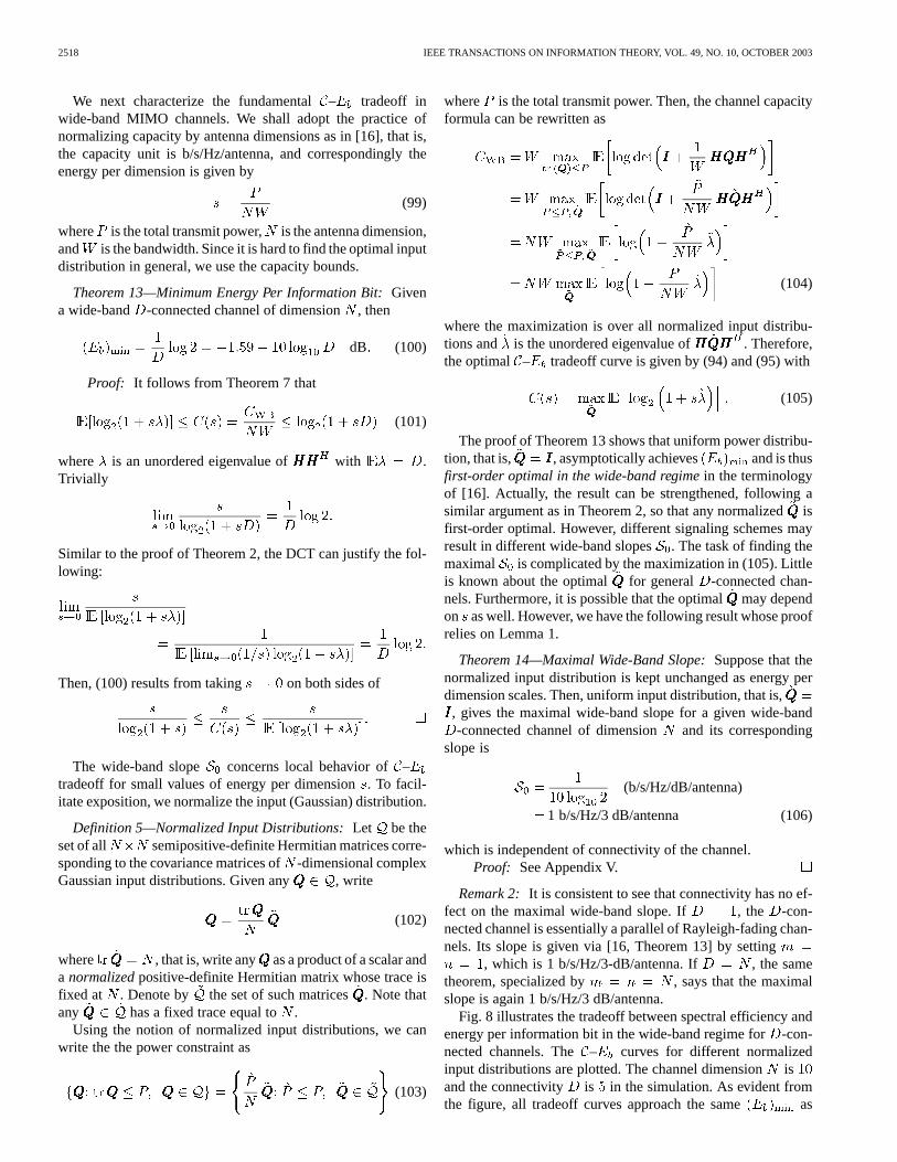
Fig. 8 illustrates the tradeoff between spectral efficiency andenergy per information bit in the wide-band regime for-con-nected channels. The– curves for different normalizedinput distributions are plotted. The channel dimensionisand the connectivity is in the simulation. As evident fromthe figure, all tradeoff curves approach the same as


Fig. 8. Spectral efficiency as a function of energy per information bit in the wide-band regime for a5-connected channel of dimension10.

determined by Theorem 13, but the uniform distribution givesthe best slope as in Theorem 14.

VII. PHYSICAL INTERPRETATION OFSCALING RESULTS

In this section, we provide a physical interpretation of thescaling results, particularly in terms of the number and spatialdistribution of propagation paths. The most important scalingresults are due to Theorems 1 and 5. For infinite connectivity,with a nonvanishing growth ratio , capacity scaleslinearly with for large with the slope between the boundsderived in the Theorem 5. For large, and thusconnectivity must also scale linearly with to sustain linearcapacity growth. Since corresponds to a fully populatedi.i.d. channel, the bounds in Theorem 5 show that the only ef-fect of is to reduce the effective asymptotic received SNR(slope of capacity growth). This is consistent with the interpre-tation that reflects the fraction of virtual receiveangle that couple with each virtual transmit angle andvice versa.However, for fixed connectivity , the capacity saturates to avalue between and because scattering is not rich enoughfor to scale with .

Recall from (46) that we need on the order ofresolvable paths to populate a-con-

nected channel with high probability. Thus, the number of pathsmust scale as (quadratically) with to supportlinear growth in capacity (and connectivity). On the other hand,the number of paths must scale as (linearly)with to support a finite connectivity () and nonvanishingbut finite asymptotic capacity. In addition to the growth inthe number of resolvable paths, the spatial distribution of thepaths is also critical from a scaling viewpoint. To see this, it

is instructive to interpret the scaling results in termschannelpower per dimension . Under the assumption thatthe power per path is constant , the total channelpower is given by

and from Proposition 2, for a -connectedchannel, where is the power in each nonvanishing virtualcoefficient ( in the analysis). Then, we have

(107)

and the bounds in Theorem 5 show that for largethe capacityis given by

SNR

(108)

where reflects the number of parallel channels andSNR is the received SNR per parallelchannel (dimension). For an infinite connectivity channel,

increases linearly with (from (107)) and SNRremains constant, leading to linear capacity scaling (from(108)). On the other hand, for fixed connectivity,remains constant and SNR , leading tocapacity saturation.

The preceding discussion leads to a general and intuitiveinterpretation of the number and spatial distribution of pathsrequired for capacity scaling. For an-dimensional channel,

resolvable paths, uniformly distributed in the diag-onal spatial bins of (see Fig. 2), are sufficient to createparallel channels. In order to keep SNR constant, we need


Fig. 9. Narrow-band capacity scaling versus the number of antennas for a channel simulated via the physical model. Three different physical scenarios are shown:fixed number of paths(N = 20), linear growth in the number of paths (N = 3N ; finite connectivityD = 3), and quadratic growth in the number ofpaths (N = 0:30 � N ; infinite connectivity = 0:3).

additional resolvable paths per parallel channel (diag-onal element of ) to couple each virtual receive (transmit)angle with transmit (receive) angles, so that

also increases linearly with . Thus, pathsare needed overall and they should be distributed in a physicalscattering environment with anonvanishing conditional an-gular spread(associated with each transmit or receive angle)to yield . The scattering environment in (44)(corresponding to a -connected model) with

and

would suffice . However, a more realistic scatteringenvironment with nonuniform but nonvanishing conditionalangular spreads ,

would also suffice. A finite connectivitychannel essentially corresponds to a “diagonal” scattering en-vironment with avanishingconditional angular spread (in (44)); it can be populated with paths to yield linearscaling in the number of parallel channels, but no matter howmany paths populate it, it cannot sustain a constant SNRsince does not scale.10 For a given fixed number of paths

(fixed ), we expect the capacity to increase linearlywith up to , saturate to a maximum around

, and then go to zero if we increase beyond

10This is related to the fact thatM(� ; � ) is concentrated on a one-dimen-sional curve in diagonal scattering.

that. Thus, represents the optimal number ofantennas—distributing power over more antennas is inefficient.

Figs. 9 and 10 illustrate narrow-band capacity scaling within a channel simulated via the physical model (6). Three dif-

ferent scattering environments are simulated: i) fixed numberof propagation paths ( ), ii) linear growth in thenumber of paths depicting finite connec-tivity, and iii) quadratic growth in the number of paths

depicting infinite connectivity. The SNR is20 dB and the power per path in all cases.

The channel was simulated according to a uniform conditionalangular density of the form (44) with ; the pathsangles were uniformly distributed over the support of the scat-tering function:

Channel capacity was approximated with the mutual informa-tion for uniform input power distribution which corresponds tothe lower bounds on capacity. As evident from Fig. 9, capacityis converging to zero for environment i), is exhibiting satura-tion for environment ii), and is showing linear growth for envi-ronment iii). Note that the lower bound in Theorem 1 for ii) is144 b/s/Hz. Fig. 10 plots the ratio for the three envi-ronments. As expected, the growth ratio is converging to zerofor both i) and ii), whereas it is stabilizing to a value near 4b/s/Hz/antenna for iii). Furthermore, the capacity growth ratein iii) closely agrees with the lower bound in (5) which yieldsa value of about for . It is also worth noting thatthe growth rate has stabilized to its asymptotic value around

corresponding to paths.


Fig. 10. Plots ofC(N)=N as a function ofN for a channel simulated via the physical model. Three different scenarios are shown: fixed number of paths(N = 20), linear growth in the number of paths (N = 3N ; finite connectivityD = 3), and quadratic growth in the number of paths (N = 0:30N ;infinite connectivity = 0:3).

We now briefly relate our results to the scaling results re-ported by Chuahet al. in [13]. The channel model assumed in[13] is one of the product type, that is,

(109)

where has i.i.d. zero-mean complex circular Gaussian entrieswith variance . The matrices and represent the spatialcorrelation at the receiver and the transmitter, respectively, andare assumed to possess a Toeplitz structure consistent with thestationary spatial statistics for ULAs identified in Section II-D.It is well known that Toeplitz matrices are diagonalized by DFTmatrices asymptotically [26]. Thus, for large

and (110)

where and are diagonal matrices consisting of the non-negative eigenvalues of and . Substituting (110) in (109)we get

(111)

where is also an i.i.d. matrix since andare unitary. Comparing (11) with (22), we can identify

(112)

as the narrow-band virtual channel matrix corresponding to themodel (109) used in [13]. However, the above matrix is a spe-cial case of the class of virtual matrices which consists of allmatrices with independent Guassian entries with arbitrary vari-ances. Furthermore, unlike the-connected channel model, theconditional and marginal angular spreads/bandwidths are al-ways the same in product correlation models, as evident from(112). As we argued above, the ratio of conditional-to-marginal

angular spreads is a key determinant of whether linear capacityscaling is possible or not. The product models will always pre-dict linear scaling, as in [13].

VIII. C ONCLUSION

We have investigated capacity scaling and spectral efficiencyin wide-band correlated MIMO channels using the virtual(Fourier) channel representation that provides an analyticalframework for relating characteristics of physical (ray tracing)models to channel statistics and capacity. In particular, forULAs, the virtual channel coefficients sample the physicalscattering environment, are approximately uncorrelated re-gardless of the correlation exhibited by the physical channel,and characterize the degrees of freedom in correlated channels(which are fewer than i.i.d. channels). The key construct behindour analysis is a -connected model for the virtual channelmatrix that was motivated via physical considerations andprovides a meaningful and tractable measure of the richnessof scattering. Our scaling results show that linear capacitygrowth with the number of antennas is possible if thenumber of resolvable paths grows quadratically with

to sustain a rich scattering environment. For linear growthin , the capacity eventually saturates. For a finite butlarge , we expect the following approximate behavior:i) linear growth for , ii) saturation between

, and decay to zero for .We showed that frequency selectivity does not affect the er-

godic capacity of wide-band channels. Thus, the wide-band ca-pacity is essentially governed by the spatial structure of thenarrow-band MIMO channel. In particular, the infinite band-width capacity scales linearly with transmit power. We studied


the spectral efficiency of wide-band-connected MIMO chan-nels and provided explicit characterizations of the minimum en-ergy per bit and the wide-band slope.

We emphasize that the-connected channel is a model forcorrelated channels based on two assumptions: i) spatial scat-tering function has a banded support (see (44)), and ii) uniformspatial power distribution.11 However, it encompasses many ex-isting models, including the product correlation model that hasbeen used in several analytical studies. Furthermore, as arguedin Section VII, it captures the essence of scaling in more gen-eral (and more realistic) scattering environments in which therichness of coupling between transmit and receive spatial di-mensions scales appropriately with. Currently, we are inves-tigating scaling behavior under less stringent assumptions on thespatial scattering function.

In closing, we believe that the simple and intuitively ap-pealing interpretation of physical scattering afforded by thevirtual representation can be fruitfully exploited in many otheraspects, including space–time code design [27], [28], channelestimation [29], and channel simulation.

APPENDIX IALTERNATIVE PROOF OFLEMMA 2

Proof: Starting with arbitrary , the eigen-decomposition ofis given by

(113)

where is a unitary matrix and is a diagonal matrix withnonnegative diagonal entries. Denoting , onehas

(114)

where the last step follows from Hadamard’s inequality [30] andis the th diagonal entry in . Then it follows from Jensen’s

inequality that

(115)

where . Then is a scaled doublystochastic matrix with scale by Lemma 1. The general upperbound then follows from the following nonlinear programming:

(116)

11We have recently begun experimental studies in collaboration with Prof.Ernst Bonek of FTW, Vienna, for experimental validation of the model.

Fig. 11. A schematic illustrating Rayleigh subchannel construction froma four-dimensional3-connected channel.x ’s and y ’s are input andoutput signals, respectively. The arrow indicates actual signals involved inconstruction. A two-dimensional subsystem is denoted by a dotted frame in thefigure.

It is easy to see that the objective function is concave and theconstraint domain is convex. The Lagrangian of the program isgiven by

(117)

Setting partial derivatives to zero we get

(118)

Observe is a solution to (118). It isalso easy to check that this solution together with associatedsatisfies the Kuhn–Tucker condition [31], and thus achieves themaximum which turns out to be .

APPENDIX IIPROOF OFLEMMA 4

Proof: We illustrate the idea by an example shown in Fig. 11where and . If the information is only transmittedat the second and third transmit antenna, the received signal atthe first and second receive antenna can be written as

(119)

Note that the effective two-dimensional MIMO channelmatrix is a lower triangular matrix with entries in the maindiagonal being complex Gaussian distributed. Similar toBLAST-type processing [32], [33], successive decoding andinterference cancellation can be used to construct two parallelRayleigh-fading subchannels. More specifically, the firstsubchannel corresponding to the first received antenna has thefollowing channel equation:


Assuming that the signal has been correctly decoded (assumingcapacity-achieving codes are used), its interference toward thesecond receive antenna can be removed as

which gives rise to the second Rayleigh-fading channel asso-ciated with the second receive antenna. Note that this methodof constructing one-dimensional subchannels has been used inmany works to analyze system capacity (see, e.g., [1]).

Generally, consider an -dimensional -connected channel.Without loss of generality, one can assumeto be an odd in-teger. A transmit antenna with indexis allowed to transmit if

Hence, the number of effective transmit antennas isAfter collecting signals from theth receive antenna with

, the effective system has a lower triangularchannel matrix with dimension . Similar to thesuccessive decoding and interference cancellation methodelaborated above, a total of parallel Rayleigh sub-channels can be formed by successive interference cancellation.The processing begins with the decoding of information sent bythe th transmit antenna at the first receive antenna.The corresponding first Rayleigh subchannel is given by

Assuming perfect decoding, the interference of the thtransmit antenna toward the next transmit antenna can be sub-tracted as

which gives rise to the second Rayleigh subchannel. This proce-dure continues until the last receive antenna has beenprocessed. Therefore, the mutual information of theparallel Rayleigh subchannels is

which provides the desired lower bound for channel capacity.

APPENDIX IIIPROOF OFTHEOREM 3

W need some results from real analysis and probabilitytheory.

Lemma 5—Fatou’s Lemma, See [23]:If then

(120)

Definition 6—Weak Convergence of Distributions:Asequence of distribution functions is said to convergeweakly to a limit (written ) if for all

that are continuity points of .

Theorem 15—(See [21]):If , then there arerandom variables , , with distribution so that

a.s.

Proposition 3: Let be equicontinuous andpointwise. If then

(121)

Proof: By Theorem 15, there exist random variablesand in some probability space , with distributionand , respectively, and It is fairly straightforwardto see that

(122)

at all for which by virtue of the equicontinuityof . Then

(123)

where we have used Fatou’s lemma in passing inside theintegral.

We now give a proof of Theorem 3.

Proof: Denote by the probability space ofrandom ESD . Let

converges to

By hypothesis, . For all , it is obvious thatand, hence, by Proposition 3

(124)

Now we apply Fatou’s lemma to get

(125)

which completes the proof.

APPENDIX IVPROOF OFTHEOREM 4

Proof: We adapt Grenander and Silverstein’s proof. Pleaserefer to the original work [14] for notations. In our case,and , that is, no random connectivity and, hence,

in our notation. We examine the LESD of .Reference [14, eq. (2, 2)] becomes

(126)The proof would be the same if one could show [14, Lemma1] holds for the complex case. The key is to break the sum in(126) into two parts: one part contributes in the limit and the


other does not. Since all the moments of a complex Gaussianrandom variable are finite, the noncontributing terms diminish.Hence, only terms that exactly pair up ’s are relevant, whichis the content of Lemma 1. A similar argument can be used toshow . Therefore, the desired conclu-sion holds.

APPENDIX VPROOF OFTHEOREM 14

Proof: Since is fixed during scaling, the capacity (mu-tual information) per dimension is given by

(127)

where is an unordered eigenvalue of . The DCT canjustify the interchange of expectation and derivatives to give

(128)

(129)

Applying Theorem 12,

(130)

which is [16, Theorem 13] specialized to our case. Our task isto evaluate for a -connected channel .

Let be the eigen-decomposition of and let. One has

(131)

Then

(132)

where we have used the scaled doubly stochastic matrix prop-erty of (Lemma 1) and the fact that

(133)

Let . We shall compute

(134)

where is the th entry of . The matrix looks like

......

... (135)

where generally

(136)

Note that is a quadratic polynomial of .We take the first row , for example, to illustrate thecomputation for the coefficients of this polynomial.

First, consider the terms like for . The coeffi-cient of the term due to the first row in is

(137)

By , different rows of are uncorrelated since entriesof are uncorrelated. Thus, if , one has

Moreover, since the entries of, and, thus, , are from apropercomplex Gaussian joint distribution, theGaussian moment-fac-toring theorem(GMFT) [34] implies that

Therefore,

(138)

where Lemma 1 is used in the last step.Next, consider the terms like for . The

coefficient due to the first row in is

(139)

Use GMFT to break the sum into two parts as

(140)


Let and be the th and th column vectors of , respec-tively. The first sum in (140) vanishes because

(141)

where we have used Proposition 2 and for .Since different rows of are uncorrelated, the second term in(140) reduces to . Therefore,

(142)

Combining (138) and (142), the polynomial due to the first rowis

(143)Similar calculation can be done for other rows. Adding all the

polynomials, one has

(144)

where we again used Lemma 1.Since is constant, it follows

from (130) that maximizing is equivalent to minimizing, which is (144) over the constraint set

(145)

Similar to the alternative proof in Lemma 2 (Appendix I), thescaled doubly stochastic property of critically estab-lishes that the uniform power distribution, that is,

, achieves the minimum and the corresponding min-imum value is

(146)

Therefore, the maximal slope is

(147)

ACKNOWLEDGMENT

The authors gratefully acknowledge Prof. Jack W. Silversteinof the Mathematics Department at the North Carolina State Uni-versity for discussions on random matrix theory and assistancewith Theorem 4.

REFERENCES

[1] G. J. Foschini and M. J. Gans, “On limits of wireless communications ina fading environment when using multiple antennas,”Wireless PersonalCommun., pp. 311–335, 1998.

[2] I. E. Telatar, “Capacity of multi-antenna Gaussian channels,” AT&T BellLabs., 1995.

[3] G. German, Q. Spencer, L. Swindlehurst, and R. Valenzuela, “Wirelessindoor channel modeling: Statistical agreement of ray tracing simula-tions and channel sounding measurements,” inProc. IEEE Int. Conf.Acoustics, Speech, and Signal Processing, 2001, pp. 2501–2504.

[4] A. F. Molisch, M. Steinbauer, M. Toeltsch, E. Bonek, and R. S. Thomä,“Capacity of MIMO systems based on measured wireless channels,”IEEE J. Select. Areas Commun., vol. 20, pp. 561–569, Apr. 2002.

[5] D. Shiu, G. Foschini, M. Gans, and J. Kahn, “Fading correlation and itseffect on the capacity of multielement antenna systems,”IEEE Trans.Commun., vol. 48, pp. 502–513, Mar. 2000.

[6] A. M. Sayeed, “Deconstructing multi-antenna fading channels,”IEEETrans. Signal Processing, vol. 50, pp. 2563–2579, Oct. 2002.

[7] S. J. Fortune, D. H. Gay, B. W. Kernighan, O. Landron, R. A. Valen-zuela, and M. H. Wright, “WiSE design of indoor wireless systems:Practical computation and optimization,”IEEE Comput. Sci. Eng., vol.2, pp. 58–68, Mar. 1995.

[8] G. J. Foschini and R. A. Valenzuela, “Initial estimation of communica-tion efficiency of indoor wireless channels,”Wireless Networks, vol. 3,no. 2, pp. 141–154, 1997.

[9] A. J. Paulraj and C. B. Papadias, “Space-time processing for wirelesscommunications,”IEEE Signal Processing Mag., vol. 14, pp. 49–83,Nov. 1997.

[10] J. Fuhl, A. F. Molisch, and E. Bonek, “Unified channel model for mobileradio systems with smart antennas,”IEE Proc. Radar, Sonar Navig., vol.145, no. 1, pp. 32–41, Feb. 1998.

[11] A. M. Sayeed and V. Veeravalli, “The essential degrees of freedom inspace-time fading channels,” inProc. 13th IEEE Int. Symp. Personal,Indoor and Mobile Radio Communications (PIMRC’02), Lisbon, Por-tugal, Sept. 2002, pp. 1512–1516.

[12] , “A virtual representation for time- and frequency-selectiveMIMO channels: A bridge between physical and statistical models,”manuscript. Available [Online] at http://dune.ece.wisc.edu; to besubmitted toIEEE Trans. Commun..

[13] V. V. C-N Chuah, D. N. C. Tse, J. M. Kahn, and R. A. Valanzuela, “Ca-pacity scaling in mimo wireless systems under correlated fading,”IEEETrans. Inform. Theory, vol. 48, pp. 637–650, Mar. 2002.

[14] U. Grenander and J. W. Silverstein, “Spectral analysis of networks withrandom topologies,”SIAM J. Appl. Math., vol. 32, no. 2, pp. 499–519,Mar. 1977.

[15] E. Biglieri, J. Proakis, and S. Shamai(Shitz), “Fading channels: Infor-mation-theoretic and communications aspects,”IEEE Trans. Inform.Theory, vol. 44, pp. 2619–2692, Oct. 1998.

[16] S. Verdú, “Spectral efficiency in the wide-band regime,”IEEE Trans.Inform. Theory, vol. 48, pp. 1319–1343, June 2002.

[17] T. L. Marzetta and B. M. Hochwald, “Capacity of a mobile multiple-an-tenna communication link in Rayleigh flat fading,”IEEE Trans. Inform.Theory, vol. 45, pp. 139–157, Jan. 1999.

[18] S. A. Jafar, S. Vishwanath, and A. Goldsmith, “Channel capacity andbeamforming for multiple transmit and receive antennas with covari-ance feedback,” inProc. IEEE Int. Conf. Communications, 2001, pp.2266–2270.

[19] E. Visotsky and U. Madhow, “Space-time transmit precoding with im-perfect feedback,”IEEE Trans. Inform. Theory, vol. 48, pp. 637–650,Mar. 2001.

[20] J. H. Kotecha and A. M. Sayeed, “On the capacity of correlated MIMOchannels,” Univ. Wisconsin-Madison, Tech. Rep., 2002.

[21] R. Durrett,Probability: Theory and Examples, 2nd ed. Belmont, CA:Wadsworth, 1996.

[22] Z. D. Bai, “Methodologies in spectral analysis of large dimensionalrandom matrices, a review,”Statist. Sinica, pp. 611–677, 1999.

[23] G. B. Folland,Real Analysis: Modern Techniques and Their Applica-tions, 2nd ed. New York: Wiley, 1999.

[24] W. Hirt and J. L. Massey, “Capacity of the discrete-time Gaussianchannel with intersymbol interference,”IEEE Trans. Inform. Theory,vol. 34, pp. 380–388, May 1988.

[25] H. Bolcskei, D. Gesbert, and A. J. Paulraj, “On the capacity of OFDM-based spatial multiplexing systems,”IEEE Trans. Commun., vol. 50, pp.225–234, Feb. 2002.

[26] R. M. Gray, “On the asymptotic eigenvalue distribution of toeplitz ma-trices,”IEEE Trans. Inform. Theory, vol. IT-18, pp. 725–730, Nov. 1972.


[27] Z. Hong, K. Liu, R. Heath, and A. Sayeed, “Spatial multiplexing in cor-related fading via the virtual channel representation,”IEEE J. Select.Areas Commun., vol. 21, pp. 856–866, June 2003.

[28] K. Liu and A. M. Sayeed, “Space-time D-block codes via the virtualMIMO channel representation,”IEEE Trans. Wireless Commun.. alsopresented at Allerton 2002 Conf., to be published.

[29] J. Kotecha and A. M. Sayeed, “Transmit signal design for optimal esti-mation of correlated MIMO channels,”IEEE Trans. Signal Processing.also presented at Allerton 2002 Conf., to be published.

[30] R. A. Horn and C. R. Johnson,Matrix Analysis. Cambridge, U.K.:Cambridge Univ. Press, 1985.

[31] O. L. Mangasarian,Nonlinear Programming. New York: McGraw-Hill, 1994.

[32] G. J. Foschini, “Layered space-time architecture for wireless commu-nication in a fading environment when using multi-element antennas,”Bell Labs. Tech. J., vol. 1, no. 2, pp. 41–59, Autumn 1996.

[33] K. Liu and A. M. Sayeed, “Improved layered space-time processing inmultiple antenna systems,” inProc. 39th Allerton Conf. Communication,Control and Computing, Allerton, IL, Oct. 2001.

[34] I. S. Reed, “On a moment theorem for complex Gaussian processes,”IRE Trans. Inform. Theory, vol. IT-8, pp. 194–195, Apr. 1962.

capacity scaling and spectral efficiency in wide-band

Documents