capillary bridges and capillary-bridge forces - uni · pdf filecapillary bridges and...
TRANSCRIPT
Capillary Bridges and Capillary-Bridge Forces 469
Chapter 11 in the book:P.A. Kralchevsky and K. Nagayama, “Particles at Fluid Interfaces and Membranes”(Attachment of Colloid Particles and Proteins to Interfaces and Formation of Two-Dimensional Arrays)Elsevier, Amsterdam, 2001; pp. 469-502.
CHAPTER 11
CAPILLARY BRIDGES AND CAPILLARY-BRIDGE FORCES
The importance of capillary bridges has been recognized for many systems and phenomena likeconsolidation of granules and soils, wetting of powders, capillary condensation and bridging inthe atomic-force-microscope measurements, etc. The capillary bridge force is oriented normallyto the plane of the three-phase contact line and consists of contributions from the capillarypressure and surface tension. The toroid (circle) approximation can be applied to quantify theshape of capillary bridges and the capillary-bridge force. More reliable results can be obtainedusing the exact profile of the capillary bridge, which is determined by the Plateau sequence ofshapes: (1) nodoid with “neck”, (2) catenoid, (3) unduloid with “neck”, (4) cylinder, (5)unduloid with “haunch”, (6) sphere and (7) nodoid with “haunch”. For the shapes (1-5) thecapillary-bridge force is attractive, it is zero for sphere (6) and repulsive for the nodoid (7).Equations connecting the radius of the neck/haunch with the contact angle and radius arederived. The procedures for shape calculations are outlined for the cases of bridges between aplane and an axisymmetric body, and between two parallel planes. In the asymptotic case, inwhich the contact angle belongs to the range 70� < �c < 90�, the elliptic integrals reduce toelementary algebraic functions and the capillary bridge can be described in terms of the toroidapproximation. Some upper geometrical and physical stability limits for the length of thecapillary bridges are considered; the latter can be established by analysis of diagrams of volumevs. pressure. Attention is paid also to the thermodynamics of nucleation of capillary bridgesbetween two solid surfaces. Two plane-parallel plates are considered as an example. Thetreatment is similar for liquid-in-gas bridges between two hydrophilic plates and for gas-in-liquid bridges between two hydrophobic plates. Nucleation of capillary bridges is possiblewhen the distance between the plates is smaller than a certain limiting value. Equations forcalculating the work of nucleation and the size of the critical (and/or equilibrium) nucleus arepresented.

Chapter 11470
11.1. ROLE OF THE CAPILLARY BRIDGES IN VARIOUS PROCESSES AND PHENOMENA
McFarlane and Tabor [1] studied experimentally the adhesion of spherical beads to a flat plate.
They established that in clean dry air the adhesion was negligible. In humid atmosphere,
however, marked adhesion was observed, particularly with hydrophilic glass surfaces. At
saturated humidity the adhesion was the same as that observed if a small drop of water was
placed between the surfaces [1], see Fig. 11.1. Similar results were obtained in the earlier
experimental studies by Budgett [2] and Stone [3]. The formation of a liquid bridge between
two solid surfaces can lead to the appearance of attractive (adhesive) force between them
owing to the decreased pressure inside the liquid bridge and the direct action of the surface
tension force exerted around the annulus of the meniscus. We should say from the very
beginning that in some cases the force due to capillary bridge can be also repulsive, see Eq.
(11.15) below. In all cases this force is perpendicular to the planes of the three-phase contact
lines (circumferences) on the solid surfaces, in contrast with the lateral capillary forces
considered in Chapters 7-10.
The importance of the capillary bridges has been recognized in many experimental and
practical systems [4]. For example, the effect of capillary bridges is essential for the assessment
of the water saturation in soils and the adhesive forces in any moist unconsolidated porous
media [5-7]; for the dispersion of pigments and wetting of powders [8]; for the adhesion of dust
and powder to surfaces [9]; for flocculation of particles in three-phase slurries [10]; for liquid-
phase sintering of fine metal and polymer particles [11,12]; for obtaining of films from latex
and silica particles [13-15]; for calculation of the capillary evaporation and condensation in
various porous media [16-19]; for estimation of the retention of water in hydrocarbon
reservoirs [20], and for granule consolidation [21,22]. The action of capillary-bridge force is
often detected in the experiments with atomic force microscopy [23-25]. The capillary-bridge
force is also one of the major candidates for explanation of the attractive hydrophobic surface
force [26-31], see Section 5.2.3 above.
Pioneering studies (both experimental and theoretical) of capillary bridges have been
undertaken by Plateau, who classified the shapes of the capillary bridges (the surfaces of

Capillary Bridges and Capillary-Bridge Forces 471
Fig. 11.1. Liquid bridge between a spherical particle and a planar solid surface.
constant mean curvature) and investigated their stability [32-34]. The study of the instability of
cylindrical fluid interfaces by Plateau was further extended by Rayleigh, who considered also
jets of viscous fluid [35-38]. The shapes of capillary bridges between two solid spheres and
between sphere and plate were experimentally investigated by McFarlane and Tabor [1], Cross
and Picknett [39], Mason et al. [40-41], Erle et al. [42]. Exact solutions of the Laplace equation
of capillarity for the respective bridges have been obtained in the works by Fisher [7], Melrose
[43], Erle [42], Orr et al. [4]. In some cases appropriate simpler approximate solutions can be
applied [4, 41, 44-46]. All these studies deal with capillary bridges between two solids.
Capillary bridges can appear also between solid and fluid phases. Taylor and Michael [47]
studied (both theoretically and experimentally) the formation and stability of holes in a sheet of
liquid, see Fig. 2.5. Forcada et al. [48] examined theoretically the appearance of a capillary
bridge, which “jumps” from a liquid film to wet the tip of the atomic force microscope.
Debregeas and Brochard-Wyart [49] investigated experimentally the nucleation and growth of
liquid bridges between a horizontal liquid interface and a horizontal solid plate at a short
distance apart. The interaction between solid particle and gas bubble, studied by Ducker et al.
[28] and Fielden et al. [50], also leads to the formation of a capillary-bridge-type meniscus.
Capillary bridges between two fluid phases are found to have crucial importance for the process
of antifoaming by dispersed oil drops by Ross [51], Garrett [52, 53], Aveyard et al. [54-56], and
Denkov et al. [57, 58]. When an oil droplet bridges between the surfaces of an aqueous film,

Chapter 11472
two scenarios of film destruction are proposed: (i) dewetting of the drop would create film
rupture [52]; (ii) the oil bridge could have a unstable configuration and film rupturing could
happen at the center of the expanding destabilized bridge [53]. The latter mechanism has been
recorded experimentally with the help of a high-speed video camera [57] and the results have
been interpreted in terms of the theory of capillary-bridge stability [58]. More about the
bridging between two fluid phases and the antifoaming action can be found in Chapter 14
below.
Many works have been devoted to the problem of capillary-bridge stability; we give a brief
review in Section 11.3.4 below. Comprehensive review articles about the progress in this field
have been published by Michael [59] and Lowry and Steen [60].
Everywhere in this chapter we consider relatively small bridges and neglect the gravitational
deformation of the meniscus.
11.2. DEFINITION AND MAGNITUDE OF THE CAPILLARY-BRIDGE FORCE
11.2.1. DEFINITION
Let us consider an axisymmetric fluid capillary bridge formed between two solid bodies, say
two parallel plates, or particle and plate (Fig. 11.1), or two particles (Fig. 11.2), or two circular
rings [47]. The presence of capillary bridge will lead to interaction between the two bodies,
which can be attractive or repulsive depending on the shape of the bridge (see below). As in the
case of lateral capillary forces (see Chapters 7 and 8) the total capillary force Fc is a sum of
contributions from the surface tension � and the meniscus capillary pressure, Pc :
Fc = F(�) + F(p) (11.1)
Due to the axial symmetry Fc is directed along the z-axis (Fig. 11.2). To calculate the force
exerted on the upper particle (Fig. 11.2) one can apply the classical Stevin approach: the upper
part of the capillary bridge (above the plane z = 0) can be considered to be “frozen” and the z-
components of the forces exerted on the system “frozen bridge + upper particle” to be
calculated. Thus one obtains F(�) = �2�r0� and F(p) = �r02Pc, and consequently,
Fc = � �(2r0� � r02 Pc), Pc � P1 � P2 (11.2)

Capillary Bridges and Capillary-Bridge Forces 473
Fig. 11.2. Sketch of the capillary bridge betweentwo axisymmetric particles or bodies. P1and P2 are the pressures inside and outsidethe bridge of length L; r0 and rc are the radiiof the neck and the contact line; �c and �are the values of the meniscus slope angle atthe contact line and at an arbitrarily chosensection AB.
In Eq. (11.2) negative Fc corresponds to attraction between the two bodies, whereas positive Fc
corresponds to repulsion. In spite of the fact that Eq. (11.2) has been obtained for the section
across the neck (or the “haunch”, see Fig. 2.6b) of the bridge, the total capillary force Fc is
independent of the choice of the cross-section. To prove that one first represents the Laplace
equation, Eq. (2.24), in the form
� d(rsin�)/dr = Pc r tan� � dz/dr (11.3)
and then integrates:
�(rsin� � r0) = 21 Pc(r2 � r0
2) (11.4)
Comparing Eqs. (11.2) and (11.4) one obtains the expression for the capillary force Fc
corresponding to an arbitrary section of the bridge, say the section AB in Fig. 11.2:
Fc = � �(2r� sin� � r2 Pc) (0 � � � �) (11.5)
Note that Eq. (11.5) can be directly obtained by making the force balance for the section AB, in
the same way as we did for the section z = 0 (Fig. 11.2). Equation (11.4) guarantees that the
result for Fc will be the same, irrespective of the choice of the cross-section. If r is chosen to be
the radius rc of the contact line at the particle surface, then � = �c is the meniscus slope angle at
the contact line:

Chapter 11474
Fc = � �(2rc� sin�c � 2cr Pc) (11.5a)
Note that the surface tension term in Eq. (11.5) always leads to attraction between the two
particles, whereas the capillary pressure term corresponds to repulsion for Pc > 0, and to
attraction for Pc < 0 (in the latter case the bridge is nodoid-shaped with a neck, see Section
11.3.1 for details.
In accordance with the Laplace equation, Eq. (2.19), the capillary pressure Pc = P1 � P2 of an
axisymmetric meniscus can be expressed as follows:
Pc = � (1/rm + 1/ra), (11.6)
where rm and ra are, respectively, the meridional and azimuthal radii of curvature. In general, rm
and ra vary from point to point and can have positive or negative sign. The sign convention
followed in this chapter corresponds to positive rm and ra for a sphere. When the capillary
bridge has small length L, but relatively large volume, then ra >> rm and Eq. (11.6) can be
written in the form
Pc � � /rm (ra >> rm) (11.7)
Since Pc = constant (the gravity deformation negligible), then Eq. (11.7) gives rm = constant,
that is the generatrix of the meniscus is a circle in this asymptotic case.
11.2.2. CAPILLARY BRIDGE IN TOROID (CIRCLE) APPROXIMATION
As shown in Chapter 2, in the case of capillary bridges the generatrix of the meniscus is usually
an arc of nodoid or unduloid, which are mathematically expressed in terms of elliptic integrals,
see Fig. 2.7 and Eqs. (2.50)�(2.52). In some special cases the meniscus can be catenoid,
cylinder or sphere, see Section 11.3.1. For the sake of estimates, in the literature the generatrix
is often approximated with an arc of circle, and correspondingly, the meniscus is described as a
part of a toroid [1, 4, 39, 41]. In the asymptotic case described by Eq. (11.7) this is the exact
profile. When the toroid approximation is used, the meridional radius rm is uniquely determined
by the boundary condition for fixed contact angle at the line of three-phase contact (the Young
equation), see e.g. Eq. (11.10) below. On the other hand, in various works the toroid
approximation is used with different definitions of the azimuthal curvature radius ra :
Capillary Bridges and Capillary-Bridge Forces 475
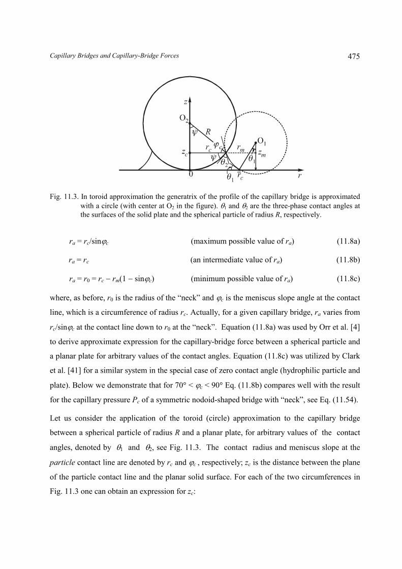
Fig. 11.3. In toroid approximation the generatrix of the profile of the capillary bridge is approximatedwith a circle (with center at O2 in the figure). �1 and �2 are the three-phase contact angles atthe surfaces of the solid plate and the spherical particle of radius R, respectively.
ra = rc/sin�c (maximum possible value of ra) (11.8a)
ra = rc (an intermediate value of ra) (11.8b)
ra = r0 = rc � rm(1 � sin�c) (minimum possible value of ra) (11.8c)
where, as before, r0 is the radius of the “neck” and �c is the meniscus slope angle at the contact
line, which is a circumference of radius rc. Actually, for a given capillary bridge, ra varies from
rc/sin�c at the contact line down to r0 at the “neck”. Equation (11.8a) was used by Orr et al. [4]
to derive approximate expression for the capillary-bridge force between a spherical particle and
a planar plate for arbitrary values of the contact angles. Equation (11.8c) was utilized by Clark
et al. [41] for a similar system in the special case of zero contact angle (hydrophilic particle and
plate). Below we demonstrate that for 70� < �c < 90� Eq. (11.8b) compares well with the result
for the capillary pressure Pc of a symmetric nodoid-shaped bridge with “neck”, see Eq. (11.54).
Let us consider the application of the toroid (circle) approximation to the capillary bridge
between a spherical particle of radius R and a planar plate, for arbitrary values of the contact
angles, denoted by �1 and �2, see Fig. 11.3. The contact radius and meniscus slope at the
particle contact line are denoted by rc and �c , respectively; zc is the distance between the plane
of the particle contact line and the planar solid surface. For each of the two circumferences in
Fig. 11.3 one can obtain an expression for zc:

Chapter 11476
R(1 � cos�) = zc = zm � rm cos�c , zm = rm cos�1 (11.9)
From Eq. (11.9) one can determine the meridional radius of curvature [4]:
rm = �R(1 � cos�)(cos�1 � cos�c)�1 (toroid approximation) (11.10)
In addition, we notice that �c = � � (� + �2) and rc = Rsin�, see Fig. 11.3. Then substituting
Eqs. (11.6), (11.8a) and (11.10) into Eq. (11.5a) one determines the capillary-bridge force in
toroid approximation:
Fc = ��R� {sin(� + �2)sin� + (1 + cos�)[cos�1 + cos(� + �2)]} (11.11a)
In the same way, but using Eq. (11.8b), instead of Eq. (11.8a), one derives an alternative
expression:
Fc = ��R� {[2sin(� + �2) � 1]sin� + (1 + cos�)[cos�1 + cos(� + �2)]} (11.11b)
A third version of the expression for Fc can be obtained combining Eq. (11.8c) with Eqs.
(11.2), (11.6) and (11.10):
Fc = ��� �
�
sincos1
a� [a sin� � (1 � cos�)(1 � sin�)](a + 1 � cos�) (11.11c)
where a � cos�1 + cos(� + �2). In spite of the different form of Eqs. (11.11a)�(11.11c) all of
them give the same asymptotics for ��0,
Fc � �2�� R(cos�1 + cos�2) = 4�� R2
cos2
cos 2121 ���� ��
(� << 1) (11.12)
which corresponds to the limiting case of a very small (thin and flat) bridge in the form of ring
around the touching point of the sphere and plane [4]. Such a “pendular ring” can be formed
between a hydrophilic sphere and a plane owing to a local condensation of water, which gives
rise to a strong adhesion [1, 61]. However, if the wetting is sufficiently imperfect that
�1 + �2 > �, then Fc has positive sign and corresponds to repulsion. For �1 = �/2 Eq. (11.12)
reduces to a formula reported by Cross and Picknett [39]. In the special case of hydrophilic
surfaces, �1 = �2 = 0, Eq. (11.11c) yields the formula derived by Haynes, see Ref. [41]:
Fc � �2�� R(2sin� + cos� � 1)/sin� (11.13)

Capillary Bridges and Capillary-Bridge Forces 477
For two equal non-zero contact angles, �1 = �2
= �, Eq. (11.12) reduces to the formula of
McFarlane & Tabor [1] Fc � �4��Rcos�. If both the sphere and plane are hydrophilic (� = 0),
then Fc � �4�R� . It is really astonishing that a tiny microscopic pendular ring, localized in the
narrow contact zone sphere-plane, can create a force equal to twice the surface tension, 2� ,
multiplied by the equatorial length of the sphere, 2�R. However, this force is not due to the
direct contribution of the surface tension, F(�) = �2�rc� sin�c. For �
� 0 the thickness of the
gap h = R(1 �
cos�) �
0, and in view of Eq. (11.10) rm �
0. In such a case, the term 1/rm
dominates the capillary pressure, Pc, and the total capillary bridge force Fc, see Eqs. (11.5a) and
(11.6). Therefore, for small pendular rings (� �
0) Eq. (11.7) holds and the toroid
approximation can be applied with a good precision.
As already mentioned, other case, in which the toroid approximation works accurately, is that
of symmetric nodoid-shaped bridges for 70� < �c
< 90�, see Eq. (11.54) below. However, to
achieve really accurate and reliable numerical results it is preferable to work with the rigorous
expressions for the capillary bridge shape, given in the next Section 11.3, and to calculate the
capillary bridge force using Eq. (11.2), or its equivalent forms (11.5) and (11.5a).
11.3. GEOMETRICAL AND PHYSICAL PROPERTIES OF CAPILLARY BRIDGES
11.3.1. TYPES OF CAPILLARY BRIDGES AND EXPRESSIONS FOR THEIR SHAPE
Let us define the dimensionless capillary pressure
p � Pc r0 /(2�) � k1r0 (11.14)
Here k1 stands for the mean curvature of the capillary meniscus. The sequence of meniscus
shapes, observed when p is increased, has been classified by Plateau [34], see Section 2.2.3 and
Table 11.1. The capillary pressure Pc can be both positive and negative; in general � < p < +.
Note that the presence of “neck” (Fig. 2.6a) not necessarily means that the capillary pressure p
is negative. Indeed, the catenoid and unduloid, corresponding to 0 �
p < 21 (Table 11.1) have
necks, but their capillary pressure is not negative, i.e. the pressure inside the bridge P1 is equal
or greater than the outside pressure P2. On the other hand, all bridges with a “haunch”
(Fig. 2.6b) have positive capillary pressure, 21 < p <
.
Chapter 11478
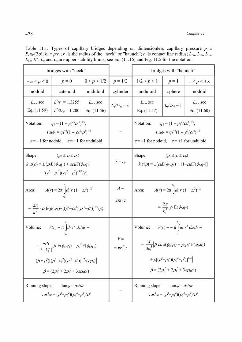
Table 11.1. Types of capillary bridges depending on dimensionless capillary pressure p �Pcr0/(2�); k1 � p/r0; r0 is the radius of the “neck” or ”haunch”; rc is contact line radius; Lnn, Lnh, Lun,Luh, L*, Lc and Ls are upper stability limits; see Eq. (11.16) and Fig. 11.5 for the notation.
bridges with “neck” bridges with “haunch”
� < p < 0 p = 0 0 < p < 1/2 p = 1/2 1/2 < p < 1 p = 1 1 < p < +
nodoid catenoid unduloid cylinder unduloid sphere nodoid
Lnn, see
Eq. (11.59)
L*/rc = 1.3255
L*/2r0 = 1.200
Lun, see
Eq. (11.56)Lc/2r0 = �
Luh, see
Eq. (11.57)Ls/2r0 = 1
Lnh, see
Eq. (11.60)
Notation: q1 = (1 � �02/�1
2)1/2,
sin�1 = q1�1(1 � �0
2/�2)1/2
� = �1 for nodoid, � = +1 for unduloid
�
Notation: q2 = (1 � �12/�0
2)1/2,
sin�2 = q2�1(1 � �2/�0
2)1/2
� = �1 for nodoid, � = +1 for unduloid
Shape: (�0 � � � �1)
|k1|z(�) = �{�1E(�1,q1) + ��0 F(�1,q1)
�[(�2 � �0
2)(�12 � �
2)]1/2/�}
r = r0
Shape: (�1 � � � �0)
k1z(�) = �[�0E(�2,q2) + (1��0)F(�2,q2)]
Area: A(r) = 2� �r
r
dr0
r (1 + zr2)1/2
= 21
2k�
{�1E(�1,q1)�[(�2��0
2)(�12��
2)]1/2/�}
A =
2�r0 z
Area: A(r) = 2� �0r
r
dr r (1 + zr2)1/2
= 21
2k�
�0 E(�2,q2)
Volume: V(r) = � �r
r
dr0
r2 dz/dr =
= ���
|| 31
1
3 kE(�1,q1) � �0
2 F(�1,q1)
� (� + �2)[(�2
��02)(�1
2��
2)]1/2/(��1)
� � (2�02 + 2�1
2 + 3��0�1)
V =
= �r02 z
Volume: V(r) = � � �0r
r
dr r2 dz/dr =
= ��
313k
�0 E(�2,q2) � �0�12 F(�2,q2)
+ �[(�2��1
2)(�02��
2)]1/2
� � (2�02 + 2�1
2 + 3��0�1)
Running slope: tan� = dz/dr
cos2� = (�2
��02)(�1
2��
2)/�2 �
Running slope: tan� = dz/dr
cos2� = (�2
��12)(�0
2��
2)/�2
Capillary Bridges and Capillary-Bridge Forces 479
With the help of Eq. (11.4) one can bring Eq. (11.2) into the form
Fc = �2�r0� (1 � p) (11.15)
For a spherical capillary bridge p = 1 and Eq. (11.15) gives zero capillary bridge force, Fc = 0.
The latter means that for a spherical bridge the repulsive capillary pressure force, F(p) = �r02Pc,
exactly counterbalances the attractive contribution of the surface tension, F(�) = �2�r0� , cf.
Eq. (11.2). The fact that if Fc = 0, then the capillary bridge must be a zone of sphere, has been
established by Mason and Clark [62].
Note also, that the nodoid with “haunch” (1 < p < ) is the only type of capillary bridge, for
which the total capillary-bridge force is repulsive, Fc > 0. On the other hand, the nodoid with
“neck” is the only type of capillary bridge, for which the capillary pressure is negative, p < 0.
To describe the shape of the capillary bridges we will use the same notation as in Section 2.2.3;
in addition, we introduce the following dimensionless variables:
� = | k1 | r, �0 = | k1 | r0, �1 = | k1 | r1, �c = | k1 | rc (11.16)
In view of Eq. (2.28) one has
�1 = | 1 � �0 sign(p) | (11.17)
where sign(p) denotes the sign of p. Then Eq. (2.48), which governs the shape of the capillary
bridge, can be represented in the form
))((tan
221
20
2
210
����
�����
��
����
drdz (11.18)
Here, as before, � is the running meniscus slope angle, see Fig. 11.2, and the parameter � = 1
is defined in Table 11.1. In addition,
�0 � � � �1 for a bridge with “neck”, (11.19a)
�1 � � � �0 for a bridge with “haunch”. (11.19b)
The integration of Eq. (11.18), in view of Eq. (11.16), yields the expressions for the generatrix
of the meniscus profile, z(�), which are given in Table 11.1; in fact, these expressions are

Chapter 11480
equivalent to Eqs. (2.50) and (2.52). The elliptic integrals of the first and second kind, F(�, q)
and E(�, q), are defined by Eq. (2.51). In the special case of catenoid the meniscus shape is
determined by Eq. (2.49). For the catenoid the meridional and azimuthal curvature radii are
equal by magnitude, | rm | = | ra
| , as it is for a sphere; however, rm = �ra. For that reason the
surface obtained by a rotation of a catenoid is sometimes termed “pseudosphere”. For a sphere
the deviatoric curvature D � 1/ra � 1/rm is constant, D � 0, whereas for a pseudosphere
D = r0/r2, i.e. it is not zero and varies from point to point.
Table 11.1 contains also expressions for the area A(r) and volume V(r) derived with the help of
Eq. (11.18). A(r) and V(r) represent, respectively, the meniscus area and the volume of a
portion of the bridge confined between the cross-sections of radii r and r0, the latter being the
section across the neck/haunch. With the help of the expressions for A(r) and V(r) given in
Table 11.1 one can determine the portions of bridge surface area and volume, A(rx, ry) and
V(rx, ry) comprised between every two sections of radii rx and ry ,
A(rx, ry) = | A(rx) ��� A(ry) | , V(rx, ry) = | V(rx) �� V(ry) | (11.20)
where the signs “�” and “+” stand, respectively, for sections situated on the same and the
opposite side(s) with respect to the section r = r0 (the neck/haunch).
11.3.2. RELATIONS BETWEEN THE GEOMETRICAL PARAMETERS
First, let us note that
�2 � �0�1 for nodoid with “neck” (11.21)
�2 � �0�1 for nodoid with “haunch” (11.22)
�2 = �0�1 inflection point for all unduloids (11.23)
In addition, from the definition of � (Table 11.1 ) and from Eq. (11.17) it follows
(�1 + ��0)2 = 1 (11.24)
Then using the identity (cos�)�2 = 1 + tan2� from Eq. (11.18) one can express the cosine of the
running slope angle:
cos2� = [(�2 � �0
2)(�12 � �2)]/�2 (11.25)
Capillary Bridges and Capillary-Bridge Forces 481
Equation (11.25), which holds for both nodoids and unduloids, can be represented also in the
form
(�0�1)2 � �2(�02 + �1
2) + �2cos2� + �4 = 0, (11.26)
which can be considered as a quadratic equation for determining �2 if �0 and � are given:
�2 = 2
1 [b (b2 � 4�02�1
2)1/2] (11.27)
b � �02 + �1
2 � cos2� = sin2
� � 2��0�1 (11.28)
The fact that Eq. (11.27) contains two roots for �2 deserves a special attention.
In the case of nodoid (�0 � �1 = 1) Eq. (11.27) has always two positive roots for �2, which in
view of Eqs. (11.21) and (11.22) correspond to the two types of nodoids:
�2 = �0�1 + 2
1 {sin2� � [(sin2
� + 4�0�1)sin2�]1/2]} (nodoid with “neck”) (11.29)
�2 = �0�1 + 2
1 {sin2� + [(sin2
� + 4�0�1)sin2�]1/2]} (nodoid with “haunch”) (11.30)
In the case of unduloid (�0 + �1 = 1) Eq. (11.27) has real roots for �2 only when
0 < �0 � sin2
2� (for unduloid with “neck”, � < �/2) (11.31)
sin2
2� � �0 < 1 (for unduloid with “haunch”, � > �/2) (11.32)
To understand the meaning of the two roots in the case of unduloids, one can express
Eq. (11.27) in the form
�2 = �0�1 + 2
1 { sin2� � 4�0�1 [(sin2
� � 4�0�1)sin2�]1/2]} (all unduloids) (11.33)
Then in view of Eq. (11.23) the two roots in Eq. (11.33) are the radial coordinates of the two
points with the same slope angle �, situated on the left and right from the inflection point of the
unduloid at �2 = �0�1.
Another possible problem, appearing when the boundary conditions for the meniscus shape are
imposed, is to determine the radius of the neck/haunch, �0, for given � and �. With that end in
view we use Eq. (11.24) to represent Eq. (11.26) in the form

Chapter 11482
u2 � 2��2u + (�4 � �2 sin2�) = 0, u � �0�1 (11.34)
Solving Eq. (11.34) for nodoid-shaped bridge one obtains u = �2 � sin�, where the roots with
“+” and “�“ correspond to meniscus with “neck” and “haunch”, respectively. Then using the
fact that for nodoid �1 = �0 1, and consequently, u = �02 �0, one derives
�0 = 21 {[1 + 4�(� + sin�)]1/2 � 1} (nodoid with “neck”) (11.35)
�0 = 21 {[1 + 4�(� � sin�)]1/2 + 1} (nodoid with “haunch”, � > sin�) (11.36)
Solving Eq. (11.34) for unduloid-shaped bridge one obtains u = ��2 + � sin� (the other root
must be disregarded). Since for nodoid u = �0 � �02, one finally derives
�0 = 21 {1 � [1 � 4�(sin� � �)]1/2} (unduloid with “neck”, � < sin�), (11.37)
�0 = 21 {1 + [1 � 4�(sin� � �)]1/2} (unduloid with “haunch”, � < sin�) (11.38)
Equations (11.37) and (11.38) yield 0 < �0 < 21 , and 2
1 < �0 < 1, respectively, which in view of
Table 11.1 determines the type of the bridge (for unduloids �0 � p).
Capillary bridge formed between axisymmetric surface and a plane. To illustrate the
application of the above equations let us consider the capillary bridge formed between a curved
axisymmetric surface of equation z = h(r) and a plane. The equation z = h(r) may represent a
sphere (see Fig. 11.3), or the shape of the cantilever of the atomic force microscope, see Refs.
[23-25, 46]. To specify the problem we assume that the contact angles �1 and �2 are known
(cf. e.g. Fig. 11.3), and that the capillary pressure Pc is negative, i.e. we deal with a nodoid-
shaped bridge with neck. Such bridges can be spontaneously formed by capillary condensation
of water between two hydrophilic surfaces at atmospheric humidity lower than 100 %;
alternatively, such bridges can be spontaneously formed by capillary cavitation of vapor-filled
bridges between two hydrophobic surfaces at temperatures lower than the boiling point of the
aqueous phase; see Section 11.4 for more details. The meniscus slope angle at the curved
surface is
�c = �2 + arctan(dh/dr) (11.39)
Capillary Bridges and Capillary-Bridge Forces 483
Then for a given (dimensionless) contact radius on the curved solid surface, �c = | k1 | rc, using
Eq. (11.35) one calculates the radius of the neck,
�0 = 21 {[1 + 4�c(�c + sin�c)]1/2 � 1}, (11.40)
of the nodoid-shaped surface; the real bridge meniscus represents a part (zone) of this surface.
With the value of �0 thus obtained from Eq. (11.29) one determines the (dimensionless) contact
radius c� at the planar solid surface:
21
2 )( cc rk�� = �0�1 + 21 {sin2
�1 � [(sin2�1 + 4�0�1)sin2
�1]1/2]} (�1 = �0 + 1) (11.41)
Further, the length of the capillary bridge (the distance between the planes of the contact lines
on the curved and planar solid surfaces) can be expressed in the form
h(rc) = | z(�c) z( c� ) | (11.42)
where the function z(�) is given in Table 11.1; the sign is “+” or “�” depending on whether the
neck appears on the real meniscus, or on its extrapolation; as already mentioned, h(r) is a
known function. Having in mind Eqs. (11.40) and (11.41) one concludes that Eq. (11.42)
relates two parameters: �c and k1, or equivalently, rc = �c / | k1 | and Pc = 2� k1. If one of them
(the contact-line radius rc, or the capillary pressure Pc) is known, then we can determine the
other one by solving numerically Eq. (11.42).
Similar procedure can be applied to the case of unduloid with neck; in the latter case one has to
use Eqs. (11.37) and (11.33) instead of Eqs. (11.40) and (11.41).
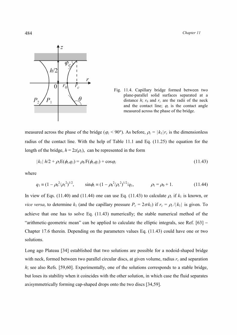
11.3.3. SYMMETRIC NODOID-SHAPED BRIDGE WITH NECK
In this subsection we consider another example of physical importance: nodoid-shaped bridge
with neck, formed between two identical parallel planar solid surfaces separated at a distance h
(Fig. 11.4). As mentioned earlier, when the liquid phase is water, an aqueous bridge can be
formed between two hydrophilic solid surfaces, or alternatively, a vapor-filled bridge can be
formed between two hydrophobic solid surfaces. In both cases we will denote by �c the
meniscus slope angle at the contact line, which represents also the three-phase contact angle
Chapter 11484
Fig. 11.4. Capillary bridge formed between twoplane-parallel solid surfaces separated at adistance h; r0 and rc are the radii of the neckand the contact line; �c is the contact anglemeasured across the phase of the bridge.
measured across the phase of the bridge (�c < 90�). As before, �c = | k1 | rc is the dimensionless
radius of the contact line. With the help of Table 11.1 and Eq. (11.25) the equation for the
length of the bridge, h = 2z(�c), can be represented in the form
| k1 | h/2 + �1E(�1,q1) = �0 F(�1,q1) + cos�c (11.43)
where
q1 � (1 � �02/�1
2)1/2, sin�1 � (1 � �02/�c
2)1/2/q1, �1 = �0 + 1. (11.44)
In view of Eqs. (11.40) and (11.44) one can use Eq. (11.43) to calculate �c if k1 is known, or
vice versa, to determine k1 (and the capillary pressure Pc = 2� k1) if rc = �c / | k1 | is given. To
achieve that one has to solve Eq. (11.43) numerically; the stable numerical method of the
“arithmetic-geometric mean” can be applied to calculate the elliptic integrals, see Ref. [63] �
Chapter 17.6 therein. Depending on the parameters values Eq. (11.43) could have one or two
solutions.
Long ago Plateau [34] established that two solutions are possible for a nodoid-shaped bridge
with neck, formed between two parallel circular discs, at given volume, radius rc and separation
h; see also Refs. [59,60]. Experimentally, one of the solutions corresponds to a stable bridge,
but loses its stability when it coincides with the other solution, in which case the fluid separates
axisymmetrically forming cap-shaped drops onto the two discs [34,59].

Capillary Bridges and Capillary-Bridge Forces 485
Let us now investigate analytically the case 70� < �c < 90�, in which the elliptic integrals can
be asymptotically expressed in terms of algebraic functions. (Note that in the case of
hydrophobic plates gas-filled bridge 70� < �c < 90� corresponds to 90� < � < 110�, where � is
the contact angle measured across water, see Fig. 11.4.) In this range of angles, which is often
experimentally observed, one has
sin�c � 1 � �2/2, � � cos�c, �2 << 1 (11.45)
The substitution of the latter expression in Eq. (11.40), after expansion in series, yields
�0 = �c � �c�2/[2(1 + 2�c)] + O(�4) (11.46)
Then one derives
(1 � �02/�c
2)1/2 = � (1 + 2�c)�1/2 + O(�3) (11.47)
With the help of Eqs. (11.17) and (11.46) one obtains:
(1 � �02/�1
2)1/2 = (1 + 2�c)1/2/(1 + �c)+ O(�2) (11.48)
Next, the combination of Eqs. (11.47) and (11.48) yields:
sin�1(�c) � (1 � �02/�c
2)1/2 (1 � �02/�1
2)�1/2 = � (1 + �c)/(1 + 2�c) + O(�3) (11.49)
One sees that sin�1(�c) = O(�) is a small quantity. Then the elliptic integrals can be expanded
in series:
F(�1,q1) = ��
1sin
022
1 sin1
�
�
�
q
d � sin�1 + O(sin3�1) � E(�1,q1) (11.50)
Eqs. (11.49) and (11.50) lead to
F(�1,q1) � E(�1,q1) � sin�1 = � (1 + �c)/(1 + 2�c) + O(�3) (11.51)
Finally, the substitution of Eq. (11.51) into Eq. (11.43) yields a simple relation between the
thickness of the gap, h, and the dimensionless radius of the contact line �c:
c
cc
kh
�
��
21||cos2
1 �
� (0 < �c < ; 70� < �c < 90�) (11.52)

Chapter 11486
Note that the above expansions for small � are uniformly valid for 0 < �c < and k1 < 0. For
�c�0 (and k1 < 0) Eq. (11.52) gives h �0, as it could be expected. In the other limit, �c�
Eq. (11.52) reduces to
||cos
1max k
h c�� (70� < �c < 90�) (11.53)
where hmax denotes the maximum possible length of the bridge (the maximum width of the gap
between the plates), for given values of the capillary pressure, Pc = 2�k1, and the contact angle
�c, the latter being measured across the bridge phase.
It is worth noting that for fixed h and �c �
0 Eq. (11.52) gives k1 �
0, but the ratio rc = �c / | k1 |
� h/(2cos�c) tends to a non-zero constant. One can obtain smaller values of rc
(i.e. rc < h/2cos�c) only using unduloid (rather than nodoid) with “neck”. It should be also
noted, that Eq. (11.52) can be presented in the alternative form
�Pc = � ���
����
��
c
c
rh1cos2 � (70� < �c < 90�) (11.54)
The comparison between Eqs. (11.54) and (11.6) shows that the meridional curvature radius is
constant: rm = �h/(2cos�c) = const. In fact, Eq. (11.54) represents the result, which would be
obtained if the “toroid” (“circle”) approximation were directly applied to express the capillary
pressure using the definition (11.8b) for the azimuthal curvature radius ra. Hence, it turns out
that the toroid approximation can be applied with a good precision to nodoid-shaped bridges
with neck, if the contact angle belongs to the interval 70� < �c < 90�.
Similar expansion for small �2 can be applied also to the case of unduloid with neck; as a
starting point one is to use Eq. (11.37) with � = �c, instead of Eq. (11.40). In first
approximation one obtains again Eq. (11.54), that is the toroid approximation.
11.3.4. GEOMETRICAL AND PHYSICAL LIMITS FOR THE LENGTH OF A CAPILLARY BRIDGE
Although derived for a special type of capillary bridge, Equation (11.53) demonstrates the
existence of limits for the length of a capillary bridge. The nodoid and unduloid are periodical
curves along the z-axis, see Figs. 2.7 and 11.5. Moreover, the nodoid has self-intersection

Capillary Bridges and Capillary-Bridge Forces 487
Fig. 11.5. Geometrical upper limits for the stability of capillary bridges: (a) distances between twoclosest points with vertical tangents for an unduloid with “neck”, Lun, and with “haunch”,Luh; (b) distances between two closest points with horizontal tangents for a nodoid with“neck”, Lnn, and with “haunch”, Lnh.
points. Unduloid-shaped bridges of length greater than the period of unduloid as a rule are
physically unstable, see Refs. [59,60]; hence the period of unduloid gives an upper limit for the
stability of the respective bridges (the longer bridges are unstable, whereas the shorter bridges
could be stable or unstable). The distance (along the z-axis) between two consecutive points
with horizontal tangent (slope angle � = 0) on the nodoid (Fig. 11.5b) can also serve as an
upper limit for the stability of nodoid-shaped bridges. Below we provide expressions for these
upper stability limits, which could be helpful for estimates.
In Fig. 11.5a the geometrical limits for the stability of the unduloids with “neck” and “haunch”
are denoted by Lun and Luh, respectively. Each of them can be identified with 2z(�1), where the
function z(�) is given in Table 11.1. In addition, for � = �1 one has sin�1 = sin�2 = 1;
consequently, �1 = �2 = �/2, and the elliptic integrals in Table 11.1 reduce to the respective total
elliptic integrals [63-66]:
K(q) � F(�/2, q), E(q) � E(�/2, q), (11.55)
Then with the help of Eqs. (11.14), (11.16), (11.17) and the expressions for z(�) in Table 11.1
one obtains
Chapter 11488
Lun(p)/(2r0) = K(q1) + p
p�1 E(q1), q1 = p
p�
�
121
for 0 < p < 21 (11.56)
Luh(p)/(2r0) = E(q2) + p
p�1 K(q2), q2 = pp 12 �
for 21 < p < 1 (11.57)
For p �
21 one has q1 = q2 = 0; in addition, K(0) = E(0) = �/2. Then from Eqs. (11.56) and
(11.57) one obtains
Lc � 2/1
lim�p
Lun(p) = 2/1
lim�p
Luh(p) = 2�r0 (11.58)
Indeed, the upper limit for the stability of a cylindrical (p = 21 ) capillary bridge of radius r0 is
Lc = 2�r0. This critical value was given first by Beer [67] and obtained in the studies by Plateau
[34]. Lc = 2�r0 is the limit of stability of the cylindrical bridge against axisymmetric
perturbations at fixed (controlled) volume of the bridge. In the case of pressure control the limit
of stability appears at two times shorter length: L = �r0, see e.g. Refs. [59,60].
For p �
1 (spherical bridge, Table 11.1) Eq. (11.57) yields Luh �
2r0; indeed, from geometrical
viewpoint the larger possible diameter of a spherical bridge is the diameter of the sphere, 2r0.
The geometrical limits for the length of a nodoid-shaped bridge (see Fig. 11.5b) can be
determined in a similar way:
),(E||1||
||1||2
),(F2 1111
0
nngggg q
pp
pp
qr
L��
��
�
�� � < p < 0 (11.59)
),(F1),(E2 2222
0
nhgggg q
ppq
rL
���
�� 0 < p < (11.60)
where q1g � (2|p| + 1)1/2(1 + |p|)�1; sin�1g � [(1 + |p|)/(2|p| + 1)]1/2; q2g � (2p � 1)1/2p�1 and
sin�2g � [p/(2p � 1)]1/2; the fact that the nodoid has horizontal tangent at � = �g � (�0�1)1/2 has
been used. For p�1 Eq. (11.60) yields Lnh� 2r0, i.e. we arrive again to the result for a sphere,
see above.
For p �
0 Eqs. (11.56) and (11.59) give divergent values for Lun and Lnn; this result can be
attributed to the fact that there are no geometrical limitations for the length of a catenoid. On
the other hand, there are physical limitations for the length of a catenoid stemming from the
Capillary Bridges and Capillary-Bridge Forces 489
boundary conditions for the Laplace equation. Plateau [34] produced a catenoid in stable
equilibrium by suspending oil on two circular rings and adjusting the volume of the oil so that
the interface across the rings was planar. He found that the catenoid thus produced was at the
limit of its stability when the distance apart of the rings L to the diameter 2rc reached a value
approximately 0.663. He recognized also that for L/2rc < 0.663 there is an alternative catenoid
solution not observable in the experiments, and that the limit of stability is reached when the
two solutions coincide; see Ref. [59] for more information.
To elucidate this point one can use the equation of the catenoid, Eq. (2.49), to obtain the
connection between the length of the bridge, L, and the contact radius rc:
rc/r0 = cosh(L/2r0) (11.61)
Introducing variables x � L/2r0 and a � L/2rc one transforms Eq. (11.61) to read
x = a cosh x (11.62)
When a is small enough the straight line y1(x) = x has two intersection points with the curve
y2(x) = a cosh x ; they represent the two roots of Eq. (11.62) corresponding to the two catenoids
recognized by Plateau. For larger values of a Eq. (11.62) has no solution. For some
intermediate critical value a = a* the line y1(x) is tangential to the curve y2(x) and the two roots
coincide; from the condition for identical tangents, y1’(x*) = y2’(x*), one obtains a*sinh x* = 1.
The combination of the last result with Eq. (11.62) yields a transcendental equation for x* :
x* = coth x* x* � L*/2r0 = 1.1996786... (11.63)
Finally, one recovers the result of Plateau: L*/2rc � a* = (sinh x*)�1 = 0.6627434... � 0.663.
The latter value determines the maximum length, L*, of the catenoid formed between two
identical circular rings of a given radius rc.
Stability of capillary bridge menisci. As mentioned above, the parameters Lun, Luh, Lc,
Lnn, Lnh and L* calculated above serve as upper limits for the length of the bridges: the longer
bridges are unstable, but the shorter bridges could be stable or unstable, depending on the
specific conditions. In general, the bridges are more stable when the volume of the bridge and
the position of the three-phase contact line are fixed. The bridges are less stable when the
pressure, rather than the volume, is fixed; see Refs. [59, 60] for a detailed review.
Chapter 11490
In general, two methods are used to investigate the stability of capillary bridges. As
demonstrated in Section 2.1.2 the Laplace equation of capillarity corresponds to an extremum
of the grand thermodynamic potential �. A solution of Laplace equation describes a stable or
unstable equilibrium meniscus depending on whether it corresponds, respectively, to a
minimum or maximum of �. Then the sign of the second variation of � is an indication for
stability or instability. This approach was applied to capillary bridges by Howe [68], and
utilized by many authors [69-71].
The second method for determining the stability of capillary menisci arose from the analysis of
the behavior of pendant and sessile drops and bubbles used in the methods for surface tension
measurements. These observations revealed that the stability limits always lie at turning points
in the plots of volume against pressure (PV-diagrams) [60]. The turning points in volume are
the points on the PV-diagram at which the volume has local minimum or maximum; they
represent stability limits in the case of fixed (controlled) volume. Likewise, the turning points
in pressure are the points on the PV-diagram at which the pressure has local minimum or
maximum; they represent stability limits in the case of fixed (controlled) pressure.
Classical example for turning points in pressure are the local extrema of pressure in the PV-
diagram predicted by the well-known van der Waals equation of state for temperatures below
the critical one; these turning points separate the unstable region from the region of
(meta)stable gas or liquid, see e.g. Ref. [72]. Another example for turning point in pressure is
observed with the known “maximum bubble pressure method” for measurement of dynamic
surface tension [73-75]; the transition from stability to instability occurs when the bubble
reaches hemispherical shape and maximum pressure [76]. Note, however, if the same system is
under volume control (say liquid drop of controlled volume instead of bubble) the turning point
in pressure is no more a stability limit: stable states beyond hemisphere can be realized. The
idea that stability changes for drops always occur at turning points was put forward as a
proposition for meniscus stability analysis by Padday & Pitt [77] and Boucher & Evans [78]. In
addition, bifurcation points on the PV-diagrams are also recognized as stability limits,
especially for relatively long capillary bridges at volume control (the bridges under pressure
control are less stable and cannot survive until the appearance of bifurcation points), see Refs.
[60,79] for details.

Capillary Bridges and Capillary-Bridge Forces 491
Fig. 11.6. Plot of the volume of a liquid bridge, V, scaled with the volume of the cylindrical bridge, Vcyl,against the dimensionless pressure difference across the meniscus surface, cP~ , see Eq. (11.64);the bridge is symmetric like that in Fig. 11.4; V and ˜ P c vary at fixed contact line radius rc andfixed length L of the bridge {after Ref. [60]}.
For example, the stability limit L = �r0 for cylindrical bridge under pressure control is a turning
point in pressure, whereas the stability limit L = 2�r0 for cylinder under volume control is a
bifurcation point [59,60].
Figure 11.6 represents a sketch of a typical PV-diagram for relatively short liquid capillary
bridges, L/rc � L*/rc = 1.3255, which are symmetric with respect to the plane of the “neck”/
“haunch”, like it is in Fig. 2.6. Moreover, it is assumed that the contact radius, rc, is fixed, but
the slope angle at the contact line, �c, can vary, cf. Fig. 11.4. The dimensionless pressure in
Fig. 11.6 is defined as follows:
cP~ � Pc rc /(2�) (11.64)
For catenoid and cylinder cP~ = p = 0 and 21 , respectively, but in general cP~ � p , cf. Eqs.
(11.14) and (11.64) (p is not suitable to be plotted on a PV-diagram, because it reflects not only
variations of the pressure Pc, but also changes in the neck radius r0). Each point on the curve in
Fig. 11.6 corresponds to a capillary bridge in mechanical equilibrium, which could be stable or
unstable. In particular, the section AB corresponds to unduloid-shaped bridges (0 < p < 21 , cf.
Table 11.1) with a very thin neck, which are unstable [60]. At the point A the neck radius r0
becomes zero and the bridge splits on two pieces of spheres. Point B is a turning point in
volume; it represents a boundary between stable bridges of controlled volume (on the left) and

Chapter 11492
the unstable bridges (on the right). Likewise, point D is a turning point in pressure: the whole
line DEFGH corresponds to stable bridges under pressure (or volume) control, whereas the
section DA corresponds to bridges unstable under pressure control. The section BD represents
bridges with neck, which are stable under volume control, but unstable under pressure control.
The points C and E, at which cP~ = p = 0, represent the two catenoids, determined by the roots
of Eq. (11.62). The catenoid bridge E (that of greater volume) is stable in both the regimes of
fixed volume and pressure, whereas the catenoid bridge C (that of smaller volume) is stable
only in the regime of fixed volume [60]. When L/rc = L*/rc = 1.3255 points C and E merge
with point D, and for L/rc > 1.3255 there are no equilibrium catenoid (and nodoid with neck)
bridges. The section EF corresponds to stable unduloid-shaped bridges with “neck”
(0 < p < 21 ), the section FG represents stable unduloid-shaped bridges with “haunch”
( 21 < p < 1), and finally, the section GH corresponds to stable nodoid-shaped bridges with
“haunch” (p > 1, cf. Table 11.1). The equilibrium bridges at the points F and G have the shape
of cylinder and truncated sphere, respectively. At the point H one has L/r0 = Lnh/r0, see
Eq. (11.60), which is the limit of stability of the menisci with “haunch” [60].
For L/rc = � the point F (cylindrical bridge) coincides with the point D (turning point in
pressure) and the cylindrical bridge loses its stability under regime of pressure control. For
L/rc > � the regions with stable bridges on the PV-diagrams become more narrow, and the PV-
diagrams (representing mostly unstable states) become more complicated, see the review by
Lowry and Steen [60].
11.4. NUCLEATION OF CAPILLARY BRIDGES
11.4.1. THERMODYNAMIC BASIS
The thermodynamics of nucleation (creation of a new phase from a supersaturated mother
phase), stems from the works of Gibbs [80] and Volmer [81], and describes the formation and
growth of small clusters from the new phase (drops, bubbles, crystals) in a process of phase
transition like condensation of vapors, cavitation (formation of bubbles) in boiling liquids,
precipitation of a solute from solution, etc. [82-86]. As a driving force of nucleation the
Capillary Bridges and Capillary-Bridge Forces 493
increased chemical potential of the molecules in the mother phase with respect to the new
phase is recognized. The nuclei of the new phase in the processes of homogeneous (bulk)
condensation and cavitation are spherical drops and bubbles. On the other hand, in the case of
heterogeneous nucleation (nucleation on a surface) the nuclei have the shape of truncated
spheres. In both cases the presence of a convex spherical liquid interface of large curvature
(small nucleus) leads to a large value of the pressure inside the nucleus, which in its own turn
increases the molecular chemical potential with respect to its value in a large phase of planar
interface. That is the reason why a necessary condition for such nuclei to appear is the initial
phase to be “supersaturated”: in the case of condensation the humidity must be slightly above
100 % ; in the case of cavitation (boiling) the equilibrium vapor pressure of the liquid to be
higher than the applied outer pressure.
The nodoid-shaped capillary bridges (as well as the concave spherical menisci in capillaries)
have negative capillary pressure and provide quite different conditions for nucleation.
Formation of nuclei with such interfacial shape makes possible the condensation to occur at
humidity markedly below 100% and the cavitation to happen when the equilibrium vapor
pressure of the liquid is considerably lower than the outer pressure. The effect of concave
menisci on nucleation was first established in the phenomenon capillary condensation, which
appears as a hysteresis of adsorption in porous solids [17, 86-88]. The experiments of
McFarlane and Tabor [1] on the adhesion of spherical beads to glass plate in humid atmosphere
give an example for nucleation of liquid capillary bridges.
The formation of nodoid-shaped cavities between two solid surfaces was examined by
Yushchenko et al. [89] and Parker et al. [90]. As already mentioned, the formation of such
cavities is proposed as an explanation of the attractive hydrophobic surface force [26-31].
As a physical example let us consider the nucleation of nodoid-shaped capillary bridges in the
narrow gap between two parallel plates (Fig. 11.4). The theoretical treatment is the same for
liquid bridges between two hydrophilic solid surfaces and for gas bridges between two
hydrophobic solid surfaces. In other words, the approach can be applied to both capillary
condensation and capillary cavitation. The work of formation of a nucleus can be expressed in
the form [82, 83, 85]:

Chapter 11494
W(rc) = Al� � 2Ac� cos�c � V(n)[P(n)(rc) � P] + N(n)[(n)(rc) � ] (11.65)
which represents the difference between the free energies of the system in the states with and
without nucleus. The meaning of the symbols and terms in Eq. (11.65) is the following. As
usual, � is the surface tension, Al denotes the area of the liquid meniscus and
Ac = �rc2 (11.66)
is the area encircled by each of the two contact lines of radius rc (Fig. 11.4). We will use rc as a
parameter which identifies the capillary bridge, just as in the theory of homogeneous nucleation
the drop/bubble radius is used to identify the spherical nuclei. The first and the second terms in
the right-hand side of Eq. (11.65) represent the work of formation of new phase boundaries
liquid/gas and solid/fluid, respectively; the third term is the mechanical work related to the
change in the pressure inside the nucleus, P(n), in comparison with the pressure P in the
ambient mother phase; (n)(r) and are chemical potentials of the molecules in the nucleus and
in the ambient mother phase; N(n) and V(n) are the number of molecules in the nucleus and its
volume. We assume that the mechanical equilibrium has been attained (the Laplace and Young
equations are satisfied); however, the bridges could be out of chemical equilibrium. In
particular, the multiplier �� cos�c in Eq. (11.65) stems from the Young equation. As in Section
11.3.3 angle �c is the three-phase contact angle measured across the bridge phase (in the case
of gas-in-liquid bridge the complementary angle, � = �
�
�c, is traditionally called ‘the contact
angle’). Depending on whether we deal with gas (vapor) or liquid bridges, the following
expressions are to be substituted:
N(n)[(n)(rc) � ] = P(n)(rc)V(n) ln[P(n)(rc)/P0] (gas bridges) (11.67)
N(n)[(n)(rc) � ] = (V(n)/Vm){[P(n)(rc)�P]Vm � kT ln(P’/P0)} (liquid bridges) (11.68)
As before, P(n) is the pressure in the nucleus (in the capillary bridge); P0 is the equilibrium
vapor pressure of a planar liquid surface at that temperature; P’ is the vapor pressure in the gas
phase surrounding a liquid-bridge nucleus; Vm is the volume per molecule in the liquid phase.
To obtain Eq. (11.67) we have used the expression for the chemical potential of the vapors
inside the nucleus, (n)(rc) = 0 + kT lnP(n)(rc), and that for the vapors which are in equilibrium
Capillary Bridges and Capillary-Bridge Forces 495
with the mother phase, = 0 + kT lnP0; 0 is a standard chemical potential; the ideal gas
equation, P(n)(rc)V(n) = N(n)kT, has been also employed.
To obtain Eq. (11.68) we have used the expressions = 0 + kT lnP’ and (n)(rc) = 0 +
kT lnP(v)(rc), where the equilibrium vapor pressure of the concave liquid bridge, P(v), is given
by the Gibbs-Thomson equation
P(v) = P0 exp(PcVm/kT) = P0 exp{ [P(n)(rc) � P]Vm / kT } (11.69)
Note that quantities like P, P0, P’, , Vm, are independent of rc.
Let us now investigate the dependence of nucleation work W on rc. Using the Gibbs-Duhem
equation for the phase of the bridge, one can write:
�V(n)dP(n)/drc + N(n)d(n)/drc = 0 (11.70)
Differentiating Eq. (11.65), along with Eqs. (11.66) and (11.70) one can derive
cdrdW = �
c
l
drdA � 4�rc�cos�c + [P � P(n)(rc)]
cdrdV )n(
+ [(n)(rc) � ]cdr
dN )n((11.71)
The meniscus area and the volume of the bridge can be expressed in the form
Al = 2� ��
2/
2/
h
h
dz r(z)(1 + rz2)1/2 V(n) = � �
�
2/
2/
h
h
dz r2(z) (11.72)
where r(z) expresses the meniscus profile in cylindrical coordinates and rz � �r/�z. Note, that in
general the meniscus profile depends on rc through the boundary condition at the contact line;
in other words r = r(z,rc). Differentiating under the sign of the integrals in Eq. (11.72) and
using integration by parts one can prove that
� c
l
drdA
+ [P � P(n)(rc)]cdr
dV )n( =
= 2� ��
���
� ��
��
���
��
�)n(
2/322/12
2/
2/ )1()1(1 PP
rr
rrrrrdz
z
zz
zc
h
h
+ 4�rc�cos�c (11.73)
where rzz � �2r/�z2. The expression in the brackets must be equal to zero because the meniscus
shape r(z) obeys the Laplace equation, Eq. (2.23). Then substituting Eq. (11.73) into
Eq. (11.71) one obtains

Chapter 11496
cdrdW = [(n)(rc) � ]
cdrdN )n(
(11.74)
In the theory of nucleation [81-86] the critical nucleus is defined as the nucleus with maximum
W. Then for the critical nucleus dW/drc = 0 and from Eq. (11.74) one obtains
(n)(rc*) = (11.75)
that is the critical nucleus of contact radius rc = rc* is in chemical equilibrium with the ambient
mother phase. In view of Eqs. (11.67) and (11.68) this yields
P(n)(rc*) = P0 (gas bridge) (11.76)
P(n)(rc*) = P � (kT/Vm)ln(P0/P’) (liquid bridge) (11.77)
P is to be identified with the atmospheric pressure. Below the boiling temperature of the liquid
(say at room temperature) one has P(n)(rc*) = P0 < P for a gas bridge; likewise, the capillary
condensation usually takes place at humidity below 100 %, i.e. P’/P0 < 1 and then Eq. (11.77)
gives also P(n)(rc*) < P. As mentioned earlier, a negative pressure difference, P(n)(rc*) � P < 0,
can be attained only in capillary bridges with generatrix nodoid (� < p < 0, see Table 11.1).
11.4.2. CRITICAL NUCLEUS AND EQUILIBRIUM BRIDGE
The dependence W = W(rc) can be calculated in the following way. For given values of �c, h
and �c, from Eqs. (11.40) and (11.43) one calculates �0 and k1. The substitution of the results in
the expressions for the area and volume of nodoid-shaped bridge with neck (Table 11.1) give
Al(rc) and V(n)(rc), where rc = �c / | k1 | . Further, in view of Eq. (11.14) the capillary pressure is
[P � P(n)(rc)] = 2� | k1 | . Finally, a substitution of the results in Eqs. (11.65)�(11.68) gives
W(rc). For the smallest values of rc the (non-equilibrium) bridges are unduloids with neck, for
which W(rc) can be calculated in a similar way, but Eq. (11.37) with � = �c must be used
instead of Eq. (11.40).
Physical interest represent situations, in which h < hmax, where hmax denotes the maximum
possible length of the bridge, see Fig. 11.4. For 70� < �c < 90� one can estimate hmax with the
help of Eq. (11.53). For example, let us consider the case of nucleation of vapor-filled bridges

Capillary Bridges and Capillary-Bridge Forces 497
Table 11.2. Values of the maximum possible length, hmax, of a vapor-filled equilibrium capillary bridgebetween two hydrophobic plates in water as a function of the contact angle � (Fig. 11.4) at temperature20�C, as predicted by Eq. (11.78).
� = � � �c 90� 94� 98� 102� 106� 110�
hmax (nm) 0 103 205 306 405 503
in water at temperature 20�C. In this case the surface tension is � = 72.75 mN/m and the
equilibrium vapor pressure of water is P0 = 2337 Pa, which is only 2.3 % of the normal
atmospheric pressure at the sea level, P = 101 325 Pa. Equation (11.53) acquires the form
hmax = 0
cos2PP
c
�
��(70� < �c < 90�) (11.78)
Table 11.2. contains numerical results for hmax calculated with the above parameters values.
One sees that hmax markedly increases when the contact angle � of the hydrophobic plate
increases beyond 90�. It is worthwhile noting that hmax is obtained from Eq. (11.52) for �c�,
that is the limit for a large bridge, whose azimuthal curvature radius is much greater than the
meridional one, ra >> rm. For such bridges rm = �h/(2cos�c) and using Eq. (11.7) one obtains
that the length of the bridge is given again by Eq. (11.78) for every �c � [0�, 90�] (that is 90� �
� � 180�). In this way Table 11.2 can be extended for � > 110�; then the maximum possible
value of the gap width, corresponding to � = 180�, is hmax = 1470 nm.
The large equilibrium bridges (for which ra >> rm) can be considered as a result of the process
of nucleation, which begins with a fluctuational formation of much smaller capillary bridges. In
the theory of nucleation the small nuclei are generally out of chemical equilibrium with the
mother phase, and this is the reason why they could spontaneously grow owing to the addition
of new molecules to the nucleus.
A typical picture, originating from the theory of homogeneous condensation (and cavitation), is
that a critical drop (bubble) exists, corresponding to a maximum of the work of nucleation W,
i.e. to a state of unstable equilibrium, see e.g. Refs. [85,86]. If a molecule is added to the
critical nucleus it begins to grow spontaneously; on the contrary, if a molecule is detached from
the critical nucleus, it spontaneously diminishes and disappears. For example, in the case of

Chapter 11498
homogeneous condensation of water vapors at 0�C and P’/P0 = 4 the radius of the critical
droplet was calculated to be about 0.85 nm [91, 86].
Let us consider now the case of nucleation (condensation or cavitation) of capillary bridges in a
narrow gap. The condition for extremum (maximum or minimum) of W determines uniquely
the pressure inside the (critical or equilibrium) nucleus, P(n), see Eqs. (11.76) and (11.77), and
the value of the parameter k1 = [P(n) � P]/(2�). Then the number of the extrema of W is equal to
the number of roots of Eq. (11.43) for the respective value of k1 and for the given thickness of
the gap, h, and contact angle �c. A maximum of W for some value of rc can be interpreted as
existence of a critical nucleus in a state of unstable equilibrium with the ambient mother phase.
A local minimum of W(rc) corresponds to a capillary bridge in state of stable equilibrium.
Additional information about the nucleation of liquid and gas capillary bridges can be found in
Refs. [90, 92].
11.5. SUMMARY
The role of capillary bridges has been recognized to be important for many systems and
phenomena such as adhesion of particles (dust, powders) to solid surfaces, consolidation of
granules and porous media, dispersion of pigments and wetting of powders, obtaining of latex
films, antifoaming, capillary condensation, bridging force in experiments with atomic force
microscope (AFM), attraction between hydrophobic surfaces, etc.
The capillary bridge force is oriented normally to the plane of the three-phase contact line and
its magnitude is determined by the contributions of the capillary pressure and the normally
resolved surface tension force, see Eq. (11.5). The simplest way to quantify the shape of the
capillary bridges and the capillary-bridge force is to use the toroid (circle) approximation
(Section 11.2.2). Like every approximation it has some limits of validity; moreover, there is an
ambiguity in the definition of the azimuthal radius of curvature, which results in different
expressions for the capillary bridge force, see Eqs. (11.8) and (11.11). For that reason more
reliable results can be obtained using the exact profile of the capillary bridge, which is
determined by the Plateau sequence of shapes: (1) nodoid with “neck”, (2) catenoid, (3)
unduloid with “neck”, (4) cylinder, (5) unduloid with “haunch”, (6) sphere and (7) nodoid with
Capillary Bridges and Capillary-Bridge Forces 499
“haunch”. The capillary-bridge force is attractive for the shapes (1-5), zero for sphere (6) and
repulsive for the nodoid (7).
Expressions for the bridge shape, area and volume are given in Table 11.1. In addition,
equations connecting the radius of the bridge neck/haunch with the contact angle and radius are
derived in Section 11.3.2. For the reader’s convenience the procedures for shape calculations
are outlined for the cases of bridges between plane and axisymmetric body, and between two
parallel planes, see Eqs. (11.39)�(11.44). It is demonstrated that in the asymptotic case, in
which the contact angle belongs to the range 70� < �c < 90� (or 90� < � < 110� for hydrophobic
plates), the elliptic integrals reduce to elementary algebraic functions and the capillary bridge
can be described in terms of the toroid approximation, see Eqs. (11.52)�(11.54).
Some upper “geometrical” stability limits for the length of the capillary bridges are related to
the distances between the points with horizontal and vertical tangents of the nodoid and
unduloid, see Eqs. (11.56)�(11.69). The limits for the length of a catenoid-shaped bridge are
connected with the possibility to satisfy the boundary conditions with this special shape, see
Eq. (11.63). The real “physical” limits for the bridge stability can be established by analysis of
diagrams of volume vs. pressure, see Fig. 11.6 and its interpretation.
Finally, we consider the thermodynamics of nucleation of capillary bridges between two solid
surfaces. Two plane-parallel plates are considered as an example. The treatment is similar for
liquid bridges between two hydrophilic plates and for gas bridges between two hydrophobic
plates; in both cases the work of nucleation is determined by Eq. (11.65). Nucleation of
capillary bridges is possible when the distance between the plates is smaller than a certain
limiting value hmax, see Eq. (11.78) and Table 11.2. Equations for calculating the work of
nucleation and the size of the critical (and/or equilibrium) nucleus are presented.
11.6. REFERENCES
1. J.S. McFarlane, D. Tabor, Proc. R. Soc. London A, 202 (1950) 224.2. H.M. Budgett, Proc. R. Soc. London A, 86 (1912) 25.3. W. Stone, Phil. Mag. 9 (1930) 610.4. F.M. Orr, L.E. Scriven, A.P. Rivas, J. Fluid Mech. 67 (1975) 723.5. W.B. Haines, J. Agric. Sci. 15 (1925) 529.

Chapter 11500
6. W.B. Haines, J. Agric. Sci. 17 (1927) 264.7. R.A. Fisher, J. Agric. Sci. 16 (1926) 492.8. P.C. Carman, J. Phys. Chem. 57 (1953) 56.9. A.D. Zimon, Adhesion of Dust and Powder, Plenum, London, 1969.10. J. Woodrow, H. Chilton, R.I. Hawes, J. Nucl. Energy B, Reactor Tech. 2 (1961) 229.11. W.D. Kingery, J. Appl. Phys. 30 (1959) 301.12. R.B. Heady, J.W. Cahn, Met. Trans. 1 (1970) 185.13. D.P. Sheetz, J. Polymer Sci. 9 (1965) 3759.14. J.W. Vanderhoff, H.L. Tarkowski, M.C. Jenkins, E.B. Bradford, J. Macromolec. Chem. 1
(1966) 361.15. A.S. Dimitrov, T. Miwa, K. Nagayama, Langmuir 15 (1999) 5257.16. R. Defay, I. Prigogine, in: Surface Tension and Adsorption, Wiley, New York, 1966; p.
217.17. D.H. Everett, in: E.A. Flood (Ed.) The Solid-Gas Interface, Vol. 2, M. Dekker, New York,
1967; p. 1055.18. J.C. Melrose, J. Colloid Interface Sci. 38 (1972) 312.19. M. Iwamatsu, K. Horii, J. Colloid Interface Sci. 182 (1996) 400.20. N.R. Morrow, J. Can. Pet. Tech. 10 (1971) 38.21. S.M. Iveson, J.D. Lister, Powder Technol. 99 (1998) 234.22. S.M. Iveson, J.D. Lister, Powder Technol. 99 (1998) 243.23. C.M. Mate, V.J. Novotny, J. Chem. Phys. 94 (1991) 8420.24. O.P. Behrend, F. Oulevey, D. Gourdon, E. Dupas, A.J. Kulik, G. Gremaud, N.A. Burnham,
Applied Physics A, 66 (1998) S219.25. H. Suzuki, S. Mashiko, Applied Physics A, 66 (1998) S1271.26. H.K. Christenson, J. Fang, J.N. Israelachvili, Phys. Rev. B, 39 (1989) 11750.27. V.S.J. Carig, B.W. Ninham, R.M. Pashley, J. Phys. Chem. 97 (1993) 10192.28. W.A. Ducker, Z. Xu, J.N. Israelachvili, Langmuir 10 (1994) 3279.29. J.C. Eriksson, S. Ljunggren, Langmuir 11 (1995) 2325.30. V.V. Yaminsky, Colloids Surf. A, 129-130 (1997) 415.31. V.V. Yaminsky, Langmuir 13 (1997) 2.32. J. Plateau, Experimental and Theoretical Researches on the Figures of Equilibrium of a
Liquid Mass Withdrawn from the Action of Gravity, in: The Annual Report of theSmithsonian Institution, Washington D.C., 1863; pp. 207-285.
33. J. Plateau, The Figures of Equilibrium of a Liquid Mass, in: The Annual Report of theSmithsonian Institution, Washington D.C., 1864; pp. 338-369.
34. J. Plateau, Statique Expérimentale et Théoretique des Liquides Soumis aux Seules ForcesMoléculaires, Gauthier-Villars, Paris, 1873.
Capillary Bridges and Capillary-Bridge Forces 501
35. Lord Rayleigh, Proc. London Math. Soc. 10 (1879) 4.36. Lord Rayleigh, Proc. R. Soc. London 29 (1879) 71.37. Lord Rayleigh, Philos. Mag. 34 (1892) 145.38. Lord Rayleigh, Philos. Mag. 34 (1892) 177.39. N.L. Cross R.G. Picknett, Particle Adhesion in the Presence of a Liquid Film, in: H.R.
Johnson and D.H. Litter (Ed.) The Mechanism of Corrosion by Fuel Impurities,Butterworths, London, 1963; p. 383.
40. G. Mason, W.C. Clark, Chem. Eng. Sci. 20 (1965) 859.41. W.C. Clark, J.M. Haynes, G. Mason, Chem. Eng. Sci. 23 (1968) 810.42. M.A. Erle, D.C. Dyson, N.R. Morrow, AIChE J. 17 (1971) 115.43. J.C. Melrose, AIChE J. 12 (1966) 986.44. W. Rose, J. Appl. Phys. 29 (1958) 687.45. N.L. Cross, R.G. Picknett, Trans. Faraday Soc. 59 (1963) 846.46. A. Marmur, Langmuir 9 (1993) 1922.47. G.I. Taylor, D.H. Michael, J. Fluid Mech. 58 (1973) 625.48. M.L. Forcada, M.M. Jakas, A. Gras-Marti, J. Chem. Phys. 95 (1991) 706.49. G. Debregeas, F. Brochard-Wyart, J. Colloid Interface Sci. 190 (1997) 134.50. M.L. Fielden, R.A. Hayes, J. Ralston, Langmuir 12 (1996) 3721.51. S. Ross, J. Phys. Colloid Chem. 54 (1950) 429.52. P.R. Garrett, J. Colloid Interface Sci. 76 (1980) 587.53. P.R. Garrett, in: P.R. Garrett (Ed.) Defoaming: Theory and Industrial Applications, M.
Dekker, New York, 1993; Chapter 1.54. R. Aveyard, P. Cooper, P.D.I. Fletcher, C.E. Rutherford, Langmuir 9 (1993) 604.55. R. Aveyard, B.P. Binks, P.D.I. Fletcher, T.G. Peck, C.E. Rutherford, Adv. Colloid
Interface Sci. 48 (1994) 93.56. R. Aveyard, J.H. Clint, J. Chem. Soc. Faraday Trans. 93 (1997) 1397.57. N.D. Denkov, P. Cooper, J.-Y. Martin, Langmuir 15 (1999) 8514.58. N.D. Denkov, Langmuir 15 (1999) 8530.59. D.H. Michael, Ann. Rev. Fluid Mech. 13 (1981) 189.60. B.J. Lowry, P.H. Steen, Proc. R. Soc. London A, 449 (1995) 411.61. J.N. Israelachvili, Intermolecular and Surface Forces, Academic Press, New York, 1992.62. G. Mason, W.C. Clark, Brit. Chem. Engng. 10 (1965) 327.63. M. Abramowitz, I.A. Stegun, Handbook of Mathematical Functions, Dover, New York,
1965.64. E. Janke, F. Emde, F. Lösch, Tables of Higher Functions, McGraw-Hill, New York, 1960.65. H.B. Dwight, Tables of Integrals and Other Mathematical Data, Macmillan Co., New York,
1961.

Chapter 11502
66. G.A. Korn, T.M. Korn, Mathematical Handbook, McGraw-Hill, New York, 1968.67. A. Beer, Ann. d. Phys. u. Chem. 96 (1855) 1; ibid. p. 210.68. W. Howe, Ph. D. Dissertation, Friedrich-Wilhelms Universität zu Berlin, 1887.69. A.D. Myshkis, V.G. Babskii, N.D. Kopachevskii, L.A. Slobozhanin, A.D. Tyuptsov, Low-
gravity Fluid Mechanics, Springer-Verlag, New York, 1987.70. L.A. Slobozhanin, J.M. Perales, Phys. Fluids A 5 (1993) 1305.71. J.C. Eriksson, S. Ljunggren, Langmuir 11 (1995) 2325.72. T.L. Hill, An Introduction to Statistical Thermodynamics, Addison-Wesley, Reading, MA,
1962.73. K.J. Mysels, Colloids Surf. 43 (1990) 241.74. T.S. Horozov, C.D. Dushkin, K.D. Danov, L.N. Arnaudov, O.D. Velev, A. Mehreteab, G.
Broze, Colloids Surf. A, 113 (1996) 117.75. S.S. Dukhin, G. Kretzschmar, R. Miller, Dynamics of Adsorption at Liquid Interfaces,
Elsevier, Amsterdam, 1995.76. G.F.C. Searle, in: Experimental Physics, Cambridge Univ. Press, Cambridge, 1934; p.128.77. J.F. Padday, A.R. Pitt, Phil. Trans. R. Soc. Lond. A 275 (1973) 489.78. E.A. Boucher, M.J.B. Evans, Proc. R. Soc. Lond. A 346 (1975) 349.79. T.I. Vogel, SIAM J. Appl. Math. 49 (1989) 1009.80. J.W. Gibbs, The Scientific Papers of J.W. Gibbs, vol. 1, Dover, New York, 1961.81. M. Volmer, Kinetik der Phasenbildung, Edwards Brothers, Ann Arbor, Michigan, 1945.82. A.I. Rusanov, Phase Equilibria and Surface Phenomena, Khimia, Leningrad, 1967 (in
Russian); Phasengleichgewichte und Grenzflächenerscheinungen, Akademie Verlag,Berlin, 1978.
83. V.P. Skripov, Metastable Liquid, Moscow, 1972 (in Russian).84. F.F. Abraham, Homogeneous Nucleation Theory, Academic Press, New York, 1974.85. E.D. Shchukin, A.V. Pertsov, E.A. Amelina, Colloid Chemistry, Moscow Univ. Press,
Moscow, 1982 (in Russian).86. A.W. Adamson, A.P. Gast, Physical Chemistry of Surfaces, 6th Edition, Wiley-
Interscience, New York, 1997.87. L.H. Cohan, J. Am. Chem. Soc. 60 (1938) 433.88. J.C.P. Broekhoff, B.G. Linsen, in: B.G. Linsen (Ed.) Physical and Chemical Aspects of
Adsorbents and Catalysts, Academic Press, New York, 1970; p. 1.89. V.S. Yushchenko, V.V. Yaminsky, E.D. Shchukin, J. Colloid Interface Sci. 96 (1983) 307.90. J.L. Parker, P.M. Claesson, P. Attard, J. Phys. Chem. 98 (1994) 8468.91. R.S. Bradley, Q. Rev. (London) 5 (1951) 315.92. P. Attard, Langmuir 16 (2000) 4455.