capillary pressure estimation and reservoir simulation · capillary pressure estimation and...

Capillary Pressure Estimation and Reservoir Simulation Rawan Haddad

Imperial College Supervisor - Tara La Force

Industry Supervisor - Marie Ann Giddins, Schlumberger

Capillary pressure is a key to accurately estimating the fluids in place by defining the distribution of reservoir fluids and the

fluids contacts. The initial state of equilibrium is ensured by correct capillary pressure determination.

Once lab capillary pressure data is provided, the data is imported into a reservoir simulator such as ECLIPSE.

The user can then apply a number of available keywords to scale the capillary pressure in order to honour other parameters

such as water saturation, porosity or permeability which are closely related to the capillary pressure.

The problem arises when the capillary pressure is scaled to a high value that the distribution of fluids no longer describes the

reservoir, initial equilibrium is unattained and the model becomes unstable with high CPU time and convergence problems.

The fluids in place are also wrongly estimated, which may be detrimental to a project’s economic target.

Furthermore; many reservoir engineering practices experience problems with estimating the water production in the transition

zone; sometimes being over estimated with early water breakthrough. Available quick fixes in the simulator set the water

saturation in the transition zone to equal the critical water saturation slowing down the water breakthrough; this however

assigns no dynamic range to the model making it unphysical with poor performance.

This project uses the Brugge model to investigate the scaling of capillary pressure performed by ECLIPSE, paying attention to

the estimation of fluids production in the transition zone.

Ten cases have been initialized and run by applying a hydrostatic equilibrium keyword; inputting a water saturation

distribution and scaling capillary pressure accordingly using an initial water saturation keyword; scaling capillary pressure as a

function of porosity and permeability using a J function keyword and end point scaling of capillary pressure curves using the

critical and connate water saturations keywords.

Applying a representative saturation height method to initialize the model using a water distribution keyword seemed to give

an efficient model with physical scaling of capillary pressure. It accurately estimated the oil in place, and matched the history

production well.

Using connate and critical water saturation to scale the capillary pressure and relative permeability curves gave an unphysical

model that overestimated the production both in and out of the transition zone, and using a function keyword underestimated

the production history.

The approach taken in this report confirms the importance of taking capillary pressure into account when performing

sensitivity analysis to match history data or initialize a model.

Acknowledgment

I would like to thank Marie Ann Giddins for giving me the opportunity to undertake this project and for her dedicated support,

expertise and guidance through many encountered technical problems and through all the long weekly meetings (despite her

rigorous schedules).

I wish to thank Dr. Charles Kossack for helpful meetings that lightened the project with brighter ideas.

I would like to thank my college supervisor, Dr Tara La Force for her supervision. I am overwhelmed to have been taught by a

truly professional group of lecturers and I appreciate the efforts of all Imperial College staff members who provided the

essentials for completing a final year project.

I would also like to thank all the staff of Schlumberger Abingdon Technology Center who have been very friendly and

supportive throughout my time of the project, especially Youcef, Rong and Chioma who have continuously taken time to share

their valuable knowledge.

Finally I would like to thank Daniel Robertson for the great support he has shown throughout the course of this project.

Contents

Acknowledgment .......................................................................................................................................................................... 2

1. Introduction ........................................................................................................................................................................... 1

2. Research Methods ................................................................................................................................................................. 2

2.1. Saturation height equations ......................................................................................................................................... 2

2.1.1. J Function ................................................................................................................................................................ 2

2.1.2. Lambda function ..................................................................................................................................................... 2

2.1.3. Skelt and Harrison Method ..................................................................................................................................... 2

2.1.4. Johnson Method ...................................................................................................................................................... 2

2.2. Simulation Model ........................................................................................................................................................ 3

2.2.1. Brugge Brief Description ........................................................................................................................................ 3

2.2.2. Keyword definitions ................................................................................................................................................ 3

3. Results ................................................................................................................................................................................... 3

3.1. Equilibration ................................................................................................................................................................ 4

3.2. SWATINIT .................................................................................................................................................................. 4

3.2.1. Saturation height methods Simulation..................................................................................................................... 5

3.3. JFUNC Keyword simulation ....................................................................................................................................... 6

3.3.1. Simple model results ............................................................................................................................................... 8

3.4. Initial water distribution using SWCR and SWL .......................................................................................................10

4. Discussion ............................................................................................................................................................................14

5. Conclusion ...........................................................................................................................................................................14

6. Recommendation .................................................................................................................................................................14

7. References ............................................................................................................................................................................16

Appendix ......................................................................................................................................................................................17

Figures

Figure 1: Relation of a single accumulation to capillary type curve (Holmes 2002) .................................................................... 1 Figure 2: left: Brugge PORO- PERM according to facies and right: Capillary Pressure curves according to regions ................. 3 Figure 3: initialized model using EQUIL ...................................................................................................................................... 4 Figure 4: Scaled capillary pressure using SWATINIT.................................................................................................................. 4 Figure 5: oil and water production rate for all SWATINIT cases ................................................................................................. 5 Figure 6: Oil recovery factor for all SWATINIT cases ................................................................................................................. 5 Figure 7: Water Saturation in the transition zone .......................................................................................................................... 6 Figure 8: Impact of using JFUNC keyword on the oil production rate and the recovery ............................................................. 7 Figure 9: Impact of using JFUNC keyword on the water production ........................................................................................... 7 Figure 10: water production in transition zone using JFUNC keyword ........................................................................................ 8 Figure 11: Scaling capillary pressure using JFUNC ..................................................................................................................... 8 Figure 12: scaled capillary pressure for cell (10, 1, 5) .................................................................................................................. 9 Figure 13: Relative permeability curve scaling using SWCR/SWL ............................................................................................11 Figure 14: comparison of water and oil production profile using SWATINIT and SWL/SWCR ...............................................11 Figure 15: water production in the transition zone using SWL/SWCR .......................................................................................12 Figure 16: Effect of ignoring capillary pressure ..........................................................................................................................12 Figure 17: random water distribution using SWATINIT and SWCR/SWL .................................................................................13 Figure 18: 10 best cases showing the field oil production rate using EQUIL with case 9 giving the closest match ....................18 Figure 19:10 best cases showing the field water production rate using EQUIL with case 9 giving the closest match ................18 Figure 20: 10 best cases showing the field oil cumulative production using EQUIL with case 9 giving the closest match ........19 Figure 21: 10 best cases showing the field water cumulative production using EQUIL with case 9 giving the closest match ...19 Figure 22:10 best cases showing oil production rate using SWATINIT, J function water distribution .......................................20 Figure 23:10 best cases showing field water production rate using STAWTINIT, J function water distribution ........................20 Figure 24:10 best cases showing oil cumulative production using SWATINIT, J function water distribution ...........................21 Figure 25:10 best cases showing water cumulative production using SWATINIT, J function water distribution.......................21 Figure 26: 10 best cases of oil production rate using SWATINIT, Skelt and Harrison saturation distribution ...........................22 Figure 27: 10 best cases for water production rate using SWATINIT, Skelt and Harrison water saturation distribution ...........22 Figure 28: 10 best cases showing oil production cumulative using SWATINIT, Skelt and Harrison water saturation distribution

.....................................................................................................................................................................................................23 Figure 29: 10 best cases showing water production cumulative using SWATINIT, Skelt and Harrison water saturation

distribution ...................................................................................................................................................................................23 Figure 30: 10 best cases showing water production rate using SWATINIT, Lambda water saturation distribution ...................24 Figure 31: 10 best cases showing oil production rate using SWATINIT, Lambda water saturation distribution ........................24 Figure 32: 10 best cases showing oil production cumulative using SWATINIT, Lambda water saturation distribution ............25 Figure 33: 10 best cases showing water production cumulative using SWATINIT, Lambda water saturation distribution ........25 Figure 34: 10 best cases showing oil production rate using SWATINIT, Johnson water saturation distribution ........................26 Figure 35: 10 best cases showing water production rate using SWATINIT, Johnson water saturation distribution ...................26 Figure 36: 10 best cases showing oil production cumulative using SWATINIT, Johnson water saturation distribution ............27 Figure 37: 10 best cases showing oil production cumulative using SWATINIT, Johnson water saturation distribution ............27 Figure 38: 10 best cases showing oil production rate using JFUNC water saturation distribution ..............................................28 Figure 39: 10 best cases showing water production rate using JFUNC water saturation distribution .........................................28 Figure 40: 10 best cases showing oil production cumulative using JFUNC water saturation distribution ..................................29 Figure 41: 10 best cases showing water production rate using JFUNC water saturation distribution .........................................29 Figure 42: best cases showing oil production rate using SWATINIT=SWL=SWCR ..................................................................30 Figure 43: best cases showing water production rate using SWATINIT=SWL=SWCR .............................................................30 Figure 44: best cases showing oil production cumulative using SWATINIT=SWL=SWCR ......................................................31 Figure 45: best cases showing water production cumulative using SWATINIT=SWL=SWCR .................................................31 Figure 46: best cases showing oil production rate using SWATINIT=SWL=SWCR, 0 capillary pressures ...............................32 Figure 47: best cases showing water production rate using SWATINIT=SWL=SWCR, 0 capillary pressure ............................32 Figure 48: best cases showing oil production cumulative using SWATINIT=SWL=SWCR, 0 capillary pressure .....................33 Figure 49: best cases showing water production cumulative using SWATINIT=SWL=SWCR, 0 capillary pressure ................33 Figure 50: best cases showing oil production rate using SWL=SWCR= a) random Sw, b) randomly distributed SWATINIT ..34 Figure 51: best cases showing water production rate using SWL=SWCR= a) random Sw, b) randomly distributed SWATINIT

.....................................................................................................................................................................................................34 Figure 52: best cases showing oil production cumulative using SWL=SWCR= a) random Sw, b) randomly distributed

SWATINIT ..................................................................................................................................................................................35 Figure 53: best cases showing water production cumulative using SWL=SWCR= a) random Sw, b) randomly distributed

SWATINIT ..................................................................................................................................................................................35

Figure 54: best cases showing oil production rate using all methods ..........................................................................................36 Figure 55: best cases showing water production rate using all methods ......................................................................................36 Figure 56: best cases showing water cumulative rate using all methods .....................................................................................37 Figure 57: best cases showing oil production cumulative using all methods ...............................................................................37 Figure 58: effect of capillary pressure scaling using PPCW ........................................................................................................38 Figure 59: oil production rate using JFUNC. PHI/K=0.0001 ......................................................................................................40 Figure 60: water production rate using JFUNC. PHI/K=0.0001 ..................................................................................................40 Figure 61: Oil production cumulative using JFUNC. PHI/K=0.0001 ..........................................................................................41 Figure 62: water production cumulative using JFUNC. PHI/K=0.0001 ......................................................................................41 Figure 63: Oil production rate using JFUNC. PHI/K=0.001.......................................................................................................42 Figure 64: water production rate using JFUNC. PHI/K=0.001 ....................................................................................................42 Figure 65: Oil production cumulative using JFUNC. PHI/K=0.001 ............................................................................................43 Figure 66: Water production cumulative using JFUNC. PHI/K=0.001 .......................................................................................43 Figure 67: Oil production rate using JFUNC. PHI/K=0.01..........................................................................................................44 Figure 68: Water production rate using JFUNC. PHI/K=0.01 .....................................................................................................44 Figure 69: Oil production cumulative using JFUNC. PHI/K=0.01 ..............................................................................................45 Figure 70: Water production cumulative using JFUNC. PHI/K=0.01 .........................................................................................45 Figure 71: Oil production rate using JFUNC. PHI/K=0.1 ...........................................................................................................46 Figure 72: Water production rate using JFUNC. PHI/K=0.1 .......................................................................................................46 Figure 73: Oil production cumulative using JFUNC. PHI/K=0.1 ................................................................................................47 Figure 74: water production cumulative using JFUNC. PHI/K=0.1 ............................................................................................47 Figure 75: Oil production rate using JFUNC. PHI/K=1 ..............................................................................................................48 Figure 76: water production rate using JFUNC. PHI/K=1 ...........................................................................................................48 Figure 77: Oil production cumulative using JFUNC. PHI/K=1 ...................................................................................................49 Figure 78: Water production cumulative using JFUNC. PHI/K=1 ..............................................................................................49 Figure 79: Oil production rate using JFUNC. Negative 0.001 slope of phi vs K .........................................................................50 Figure 80: Water production rate using JFUNC. Negative 0.001 slope of phi vs K ....................................................................50 Figure 81: Oil production cumulative using JFUNC. Negative 0.001 slope of phi vs K .............................................................51 Figure 82: water production cumulative using JFUNC. Negative 0.001 slope of phi vs K .........................................................51 Figure 83: Oil production rate using JFUNC. Brugge POROPERM relationship .......................................................................52 Figure 84: Water production rate using JFUNC. Brugge POROPERM relationship ...................................................................52 Figure 85: Oil production cumulative using JFUNC. Brugge POROPERM relationship ............................................................53 Figure 86: Water production cumulative using JFUNC. Brugge POROPERM relationship .......................................................53 Figure 87: Oil production rate using JFUNC. Average layered Brugge POROPERM relationship ............................................54 Figure 88: Water production rate using JFUNC. Average layered Brugge POROPERM relationship........................................54 Figure 89: Oil production cumulative using JFUNC. Average layered Brugge POROPERM relationship.................................55 Figure 90: water production cumulative using JFUNC. Average layered Brugge POROPERM relationship .............................55

Tables

Table 1: PCW for all Saturation height cases................................................................................................................................ 6 Table 2: Water saturation distribution using JFUNC .................................................................................................................... 9 Table 3: Effect of using JFUNC on the recovery factor ................................................................................................................ 9 Table 4: PCW values for JFUNC based on a PORO-PERM .......................................................................................................10 Table 5: Initial water saturation distribution using JFUNC keyword cases. ................................................................................39 Table 6: Capillary pressure at the first time step using JFUNC keyword cases ...........................................................................39 Table 7:SWATINIT cases performance .......................................................................................................................................56 Table 8:SWL/SWCR cases performance .....................................................................................................................................56

1

1. Introduction

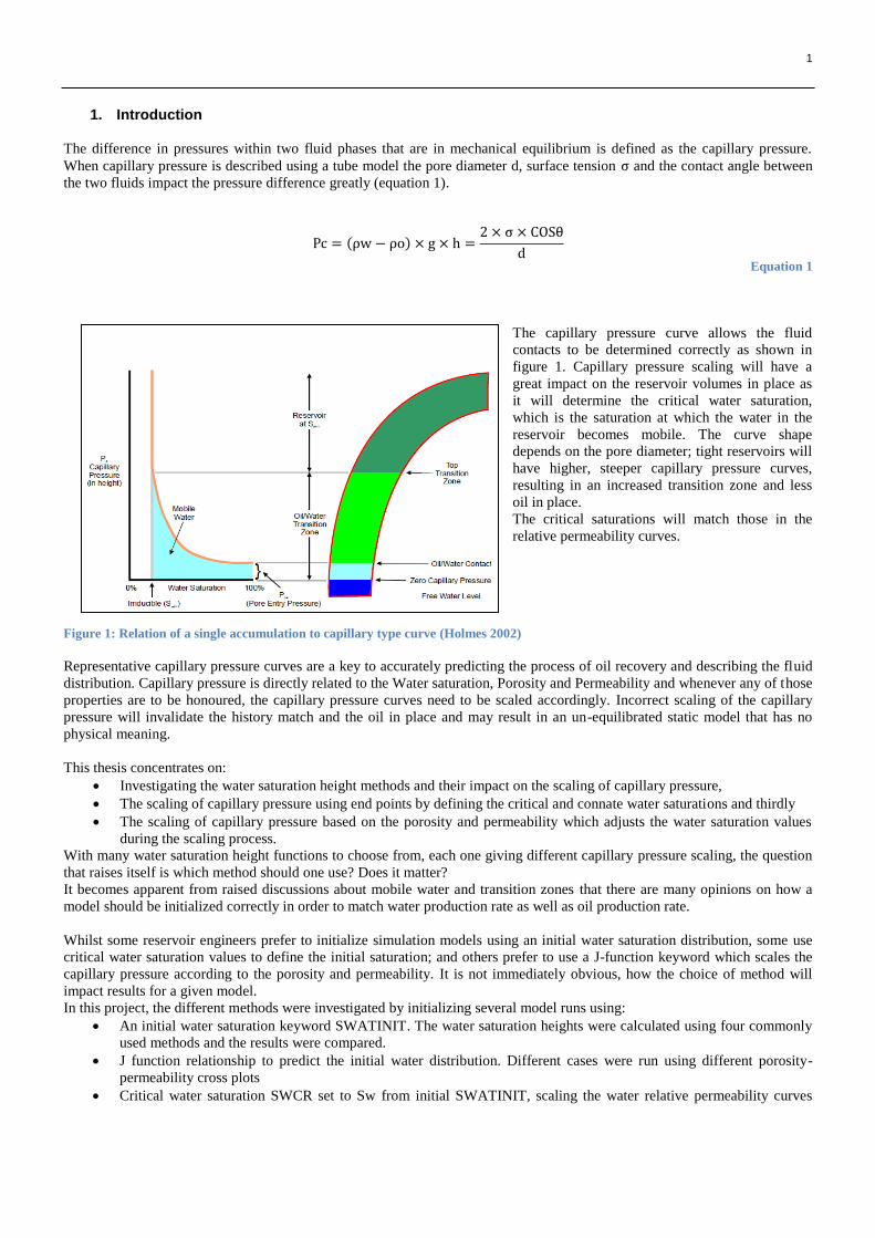
The difference in pressures within two fluid phases that are in mechanical equilibrium is defined as the capillary pressure.

When capillary pressure is described using a tube model the pore diameter d, surface tension and the contact angle between

the two fluids impact the pressure difference greatly (equation 1).

Equation 1

The capillary pressure curve allows the fluid

contacts to be determined correctly as shown in

figure 1. Capillary pressure scaling will have a

great impact on the reservoir volumes in place as

it will determine the critical water saturation,

which is the saturation at which the water in the

reservoir becomes mobile. The curve shape

depends on the pore diameter; tight reservoirs will

have higher, steeper capillary pressure curves,

resulting in an increased transition zone and less

oil in place.

The critical saturations will match those in the

relative permeability curves.

Figure 1: Relation of a single accumulation to capillary type curve (Holmes 2002)

Representative capillary pressure curves are a key to accurately predicting the process of oil recovery and describing the fluid

distribution. Capillary pressure is directly related to the Water saturation, Porosity and Permeability and whenever any of those

properties are to be honoured, the capillary pressure curves need to be scaled accordingly. Incorrect scaling of the capillary

pressure will invalidate the history match and the oil in place and may result in an un-equilibrated static model that has no

physical meaning.

This thesis concentrates on:

Investigating the water saturation height methods and their impact on the scaling of capillary pressure,

The scaling of capillary pressure using end points by defining the critical and connate water saturations and thirdly

The scaling of capillary pressure based on the porosity and permeability which adjusts the water saturation values

during the scaling process.

With many water saturation height functions to choose from, each one giving different capillary pressure scaling, the question

that raises itself is which method should one use? Does it matter?

It becomes apparent from raised discussions about mobile water and transition zones that there are many opinions on how a

model should be initialized correctly in order to match water production rate as well as oil production rate.

Whilst some reservoir engineers prefer to initialize simulation models using an initial water saturation distribution, some use

critical water saturation values to define the initial saturation; and others prefer to use a J-function keyword which scales the

capillary pressure according to the porosity and permeability. It is not immediately obvious, how the choice of method will

impact results for a given model.

In this project, the different methods were investigated by initializing several model runs using:

An initial water saturation keyword SWATINIT. The water saturation heights were calculated using four commonly

used methods and the results were compared.

J function relationship to predict the initial water distribution. Different cases were run using different porosity-

permeability cross plots

Critical water saturation SWCR set to Sw from initial SWATINIT, scaling the water relative permeability curves

2

accordingly.

The SPE Brugge benchmark model will be used to demonstrate the impact of scaling capillary pressure on the model’s

performance and output. Details of the Brugge field simulation can be found in SPE 119094. (E. Peters 2009)

Based on the results, a further attempt at recommending best industry practices is discussed.

2. Research Methods 2.1. Saturation height equations

2.1.1. J Function

In 1941, M.C. Leverett described a concept of a characteristic distribution of interfacial two-fluid curvatures with water

saturation. He described an “experimental determination of the curvature saturation relation for clean unconsolidated sand”.

(M.C.Leverette 1941).The relationship was based on the permeability and porosity of the rock sample.

Equation 2

Equation 2 is in a dimensionless form which attempts to convert all capillary pressure data, as a function of water saturation to

a universal curve. This however fails when more than one rock type is present and therefore a separate J function would have

to be used for each region.

The J function for each region can be plotted against the normal water saturation and the correlation can be described as a

power law (Adel Ibrahim 1992) in the form of:

Equation 3

Where

Equation 4

2.1.2. Lambda function

Lambda function was introduced to represent water saturation heights in thick transition zone. The Lambda function has the

following form (Nick A. Wiltgen 2003):

Equation 5

To ensure that each region’s water saturation is distributed correctly a Lambda function can be used for each region

.

2.1.3. Skelt and Harrison Method

This is a log based method that correlates water saturation and the free water level using four constants. This method is useful

for characterizing an extensive transition zone by applying a weighting factor based on the amount of gross rock area each data

point controls. This method works on both SCAL based capillary pressure and log based water saturation domain. (Harrison

1995)

The equation has the form below:

Equation 6

2.1.4. Johnson Method

This is a mathematical relationship between water saturation derived from standard laboratory capillary pressure

measurements and the permeability. The relationship is described bi-logarithmically as shown below. (Johnson 1992):

3

Equation 7

2.2. Simulation Model

The SPE Brugge benchmark model will be used to demonstrate the impact of scaling capillary pressure on the model’s

performance and output. It has seven regions sorted using the porosity. It has 30 producers and injectors and all producers are

drilled above the Oil Water Contact. The stock tank oil in place for the truth case is given as 775MBbl. Details of the Brugge

field simulation can be found in SPE 119094. (E.Peters 2009)

This simulation has been performed using ECLIPSE and Petrel RE

2.2.1. Brugge Brief Description

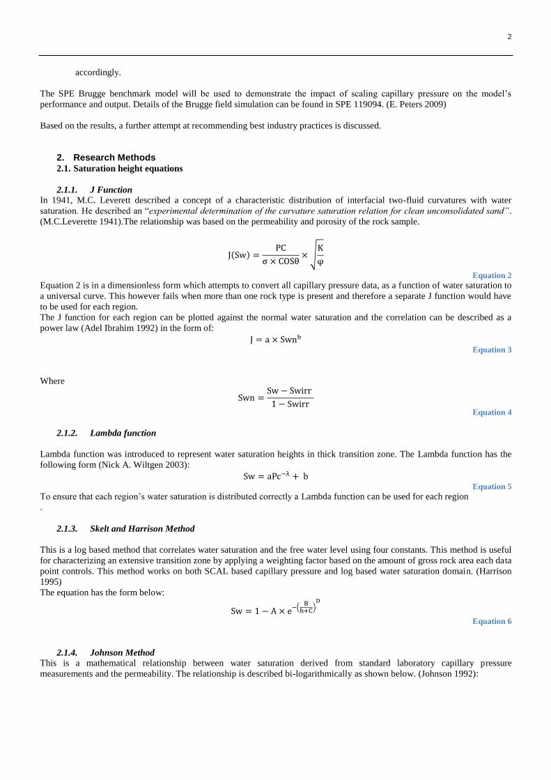
The Brugge field is a two phase synthetic oil field, consisting of oil and water. The model consists of 64000up-scaled grid

cells. The facies are subdivided into 5 classes and the PORO-PERM characteristics are shown in (figure 2 left). The reservoir

is also split into seven regions corresponding to their porosity average. (fig 2 right)

2.2.2. Keyword definitions

The following simulator keywords and their definitions are of significance on this report and will be referred to throughout the

report:

EQUIL: sets the contacts and pressures for conventional hydrostatic equilibrium.

SWATINIT: Allows the input of water saturation distribution and the scaling of the water oil capillary pressure

curves such that the water distribution is honoured in the equilibrated initial solution.

SWOF: input tables of water relative permeability, oil in water relative permeability and water oil capillary pressure

as a function of water saturation

SWL: Specifies the connate water saturation. That is the smallest water saturation in a water saturation function table

(SWOF).

SWCR: Specifies the critical water saturation. That is the largest water saturation for which the water relative

permeability is zero.

3. Results

104 realizations have been run changing the porosities and permeabilities each time. 10 best cases have been chosen based on

Figure 2: left: Brugge PORO- PERM according to facies and right: Capillary Pressure curves according to regions

4

0E+00

5E+03

1E+04

2E+04

2E+04

3E+04

3E+04

4E+04

4E+04

5E+04

01/01/98 06/24/03 12/14/08 06/06/14

Liq

uid

Flo

wra

te (

STB/d

)

Field Oil production rate

Observed 1

EQUIL_BCENTERED

the history match and the fluid in place for the purpose of analyzing the results of this report. The case discussed in the main

body of this report is case 9, the results for the other 9 cases are provided in the Appendix, Figures 19-53, showing water and

oil production rate and cumulative volume.

3.1. Equilibration

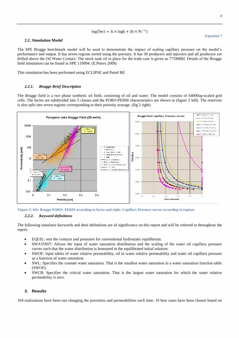
The Brugge field was first initialized using EQUIL

keyword. The contacts, datum depth and pressure are

specified, hydrostatic equilibrium is assumed and the phase

densities are then calculated using the equation of state for

oil which allows the hydrostatic pressure of the oil phase to

be calculated using equation 1. This is an iterative method

solved for oil phase pressure everywhere. Sw is then set by

reverse lookup of the capillary pressure curves supplied in

the SWOF table.

In Figure 3, the blue dotted line shows the simulation

results of an initialized model using the keyword EQUIL.

The phase pressures are calculated at 100 depth points

evenly distributed throughout the reservoir and water

saturation is assigned to each cell center.

Fig 3 shows that the history match obtained is good in the

first 10 years and starts to diverge in the second part. A

recovery factor of 0.212 is given for this method at the end

of the prediction period which is compared against other

methods used later on in the report. This model has been

run without any wells to check equilibrium state initially

and showed zero fluid displacement suggesting equilibrium

state.

3.2. SWATINIT

When the initial water saturation obtained from a geological model needs to be honoured, the initial distribution can be input

into the simulator using the SWATINIT keyword and the tabular capillary pressure curves given in SWOF tables are scaled

accordingly.

The capillary pressure is given by:

Equation 8

Where Pct is the capillary pressure value from the SWOF table and Pcm is the maximum capillary pressure value from the

table.

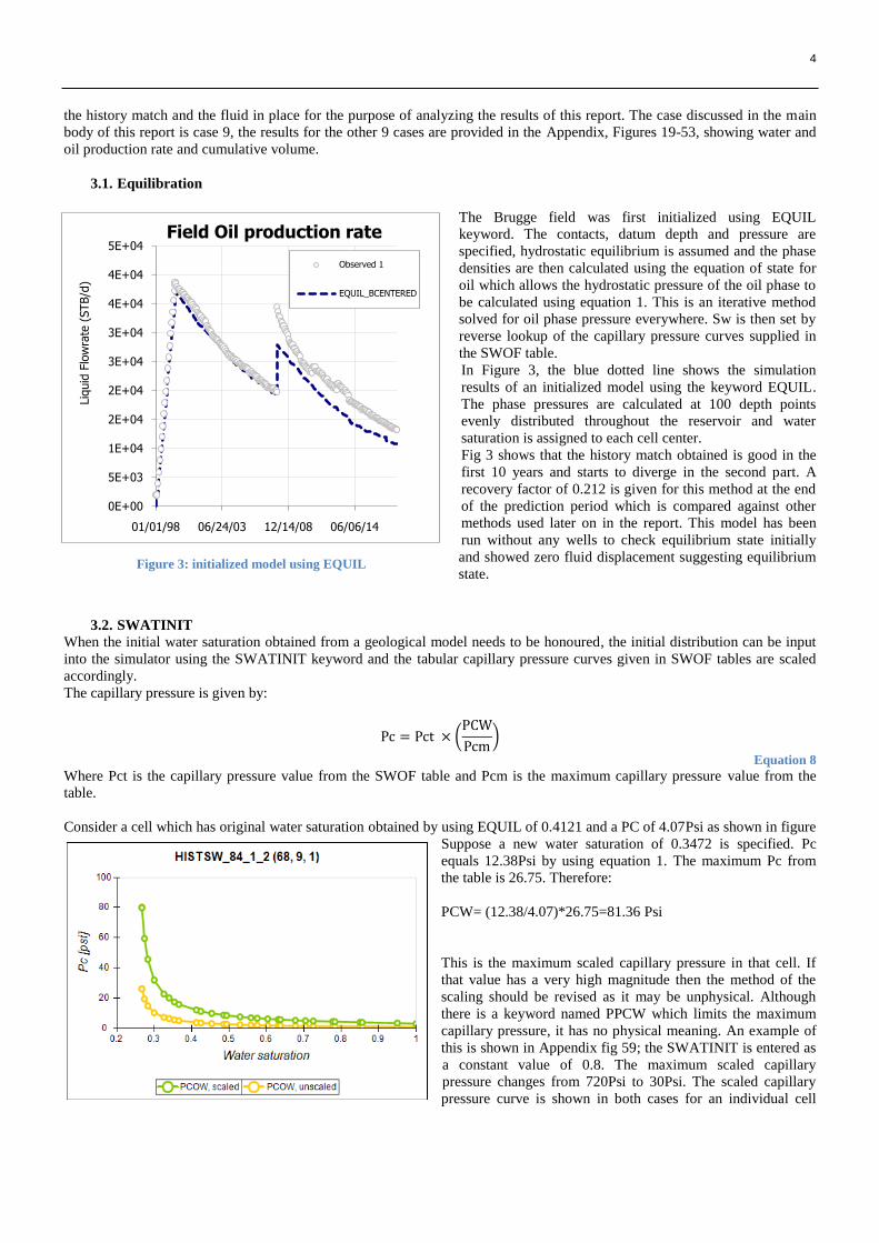
Consider a cell which has original water saturation obtained by using EQUIL of 0.4121 and a PC of 4.07Psi as shown in figure

Suppose a new water saturation of 0.3472 is specified. Pc

equals 12.38Psi by using equation 1. The maximum Pc from

the table is 26.75. Therefore:

PCW= (12.38/4.07)*26.75=81.36 Psi

This is the maximum scaled capillary pressure in that cell. If

that value has a very high magnitude then the method of the

scaling should be revised as it may be unphysical. Although

there is a keyword named PPCW which limits the maximum

capillary pressure, it has no physical meaning. An example of

this is shown in Appendix fig 59; the SWATINIT is entered as

a constant value of 0.8. The maximum scaled capillary

pressure changes from 720Psi to 30Psi. The scaled capillary

pressure curve is shown in both cases for an individual cell

Figure 3: initialized model using EQUIL

Figure 4: Scaled capillary pressure using SWATINIT

5

0.E+00

5.E+03

1.E+04

2.E+04

2.E+04

3.E+04

3.E+04

4.E+04

4.E+04

5.E+04

01/01/98 06/24/03 12/14/08 06/06/14

Liq

uid

Flo

wra

te (

ST

B/d

)


J function

EQUIL

Johnson

Skelt and Harrison

Lambda

Development strategy 1

0.E+00

5.E+03

1.E+04

2.E+04

2.E+04

3.E+04

3.E+04

01/01/98 06/24/03 12/14/08 06/06/14

Liq

uid

Flo

wra

te (

ST

B/d

)

Field Water production rate

-8.6E-15

0.05

0.1

0.15

0.2

0.25

01/01/98 09/27/00 06/24/03 03/20/06 12/14/08 09/10/11 06/06/14 03/02/17

Oil

recovery

eff

icie

ncy

Field Oil recovery efficiency

LAMBDA JFUNC

SKELT JOHNSON

EQUIL

observed

when it is limited to 30Psi cells above the oil water contact which originally had high water saturations are now forced to have

a water saturation corresponding to 30Psi pressure. In fact by applying the PPCWMAX key word the water saturation

distribution is no longer honoured. SWATINIT affects the relative permeability curves therefore it is important to make sure

that the lowest input water saturation is higher than or equal to the critical water saturation. This issue is revisited in part 2.4 of

the report.

The next section investigates the effect of using the common four methods described earlier on the Brugge reservoir

simulation and performance.

3.2.1. Saturation height methods Simulation

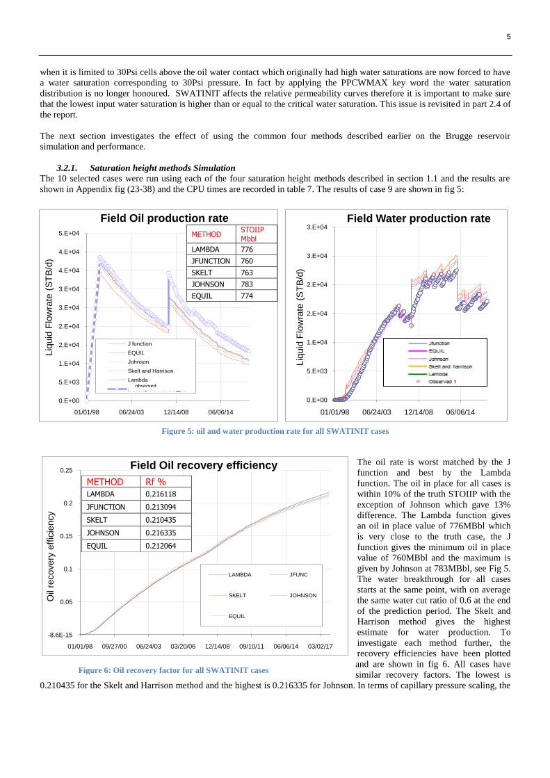
The 10 selected cases were run using each of the four saturation height methods described in section 1.1 and the results are

shown in Appendix fig (23-38) and the CPU times are recorded in table 7. The results of case 9 are shown in fig 5:

The oil rate is worst matched by the J

function and best by the Lambda

function. The oil in place for all cases is

within 10% of the truth STOIIP with the

exception of Johnson which gave 13%

difference. The Lambda function gives

an oil in place value of 776MBbl which

is very close to the truth case, the J

function gives the minimum oil in place

value of 760MBbl and the maximum is

given by Johnson at 783MBbl, see Fig 5.

The water breakthrough for all cases

starts at the same point, with on average

the same water cut ratio of 0.6 at the end

of the prediction period. The Skelt and

Harrison method gives the highest

estimate for water production. To

investigate each method further, the

recovery efficiencies have been plotted

and are shown in fig 6. All cases have

similar recovery factors. The lowest is

0.210435 for the Skelt and Harrison method and the highest is 0.216335 for Johnson. In terms of capillary pressure scaling, the

METHOD STOIIP Mbbl

LAMBDA 776

JFUNCTION 760

SKELT 763

JOHNSON 783

EQUIL 774

METHOD Rf %

LAMBDA 0.216118

JFUNCTION 0.213094

SKELT 0.210435

JOHNSON 0.216335

EQUIL 0.212064

Figure 5: oil and water production rate for all SWATINIT cases

Figure 6: Oil recovery factor for all SWATINIT cases

6

0

500

1000

1500

2000

2500

01/01/98 06/24/03 12/14/08 06/06/14

Liq

uid

Flo

wra

te (

ST

B/d

)

BR-P-15;Tubing 1

Water production rate (STB/d) lambda

Water production rate (STB/d) Development strategy 1Oil production rate (STB/d) lambda

Oil production rate (STB/d) Development strategy 1

Sw Lambda=0.6

Sw logs=0.57

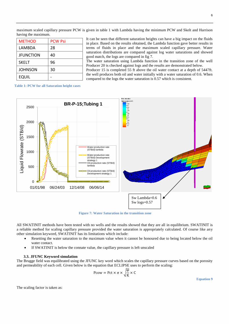
maximum scaled capillary pressure PCW is given in table 1 with Lambda having the minimum PCW and Skelt and Harrison

having the maximum.

It can be seen that different saturation heights can have a big impact on the fluids

in place. Based on the results obtained, the Lambda function gave better results in

terms of fluids in place and the maximum scaled capillary pressure. Water

saturation distributions are compared against log water saturations and showed

good match, the logs are compared in fig 7.

The water saturation using Lambda function in the transition zone of the well

Producer 20 is checked against logs and the results are demonstrated below.

Producer 15 is completed 55 ft above the oil water contact at a depth of 5447ft.

the well produces both oil and water initially with a water saturation of 0.6. When

compared to the logs the water saturation is 0.57 which is consistent.

All SWATINIT methods have been tested with no wells and the results showed that they are all in equilibrium. SWATINIT is

a reliable method for scaling capillary pressure provided the water saturation is appropriately calculated. Of course like any

other simulation keyword, SWATINIT has its limitations which include:

Resetting the water saturation to the maximum value when it cannot be honoured due to being located below the oil

water contact.

If SWATINIT is below the connate value, the capillary pressure is left unscaled

3.3. JFUNC Keyword simulation

The Brugge field was equilibrated using the JFUNC key word which scales the capillary pressure curves based on the porosity

and permeability of each cell. Given below is the equation that ECLIPSE uses to perform the scaling:

Equation 9

The scaling factor is taken as:

METHOD PCW Psi

LAMBDA 28

JFUNCTION 40

SKELT 96

JOHNSON 30

EQUIL -

Table 1: PCW for all Saturation height cases

Figure 7: Water Saturation in the transition zone

7

0.E+00

5.E+03

1.E+04

2.E+04

2.E+04

3.E+04

3.E+04

4.E+04

4.E+04

01/01/98 06/24/03 12/14/08 06/06/14

Liq

uid

Flo

wra

te (

ST

B/d

)


Equil

Jfunc

Johnson

Skelt Harrison

LAmbda

Jfunction

Development strategy 1

0

0.05

0.1

0.15

0.2

0.25

01/01/98 06/24/03 12/14/08 06/06/14

Oil

reco

ve

ry e

ffic

ien

cy


JFUNC

Johnson

Skelt and Harrison

Lambda

Jfunction

0

0.1

0.2

0.3

0.4

0.5

0.6

0.7

0.8

0.9

01/01/98 06/24/03 12/14/08 06/06/14

Liq

uid

To

Liq

uid

Ratio

(ST

B/S

TB

)

Field Water cut

Equil

JFUNC

Johnson

Skelt and Harrison

Lambda

J function

Observed 1

0.E+00

1.E+04

2.E+04

3.E+04

4.E+04

01/01/98 06/24/03 12/14/08 06/06/14

Oil

reco

ve

ry e

ffic

ien

cy


EQUILJFUNCJohnsonSkelt and HarrisonLambdaJfunctionObserved 1JFUNC

observed

Equation 10

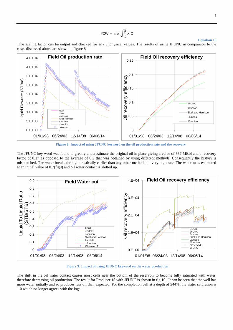
The scaling factor can be output and checked for any unphysical values. The results of using JFUNC in comparison to the

cases discussed above are shown in figure 8

The JFUNC key word was found to greatly underestimate the original oil in place giving a value of 557 MBbl and a recovery

factor of 0.17 as opposed to the average of 0.2 that was obtained by using different methods. Consequently the history is

mismatched. The water breaks through drastically earlier than any other method at a very high rate. The watercut is estimated

at an initial value of 0.7(fig9) and oil water contact is shifted up.

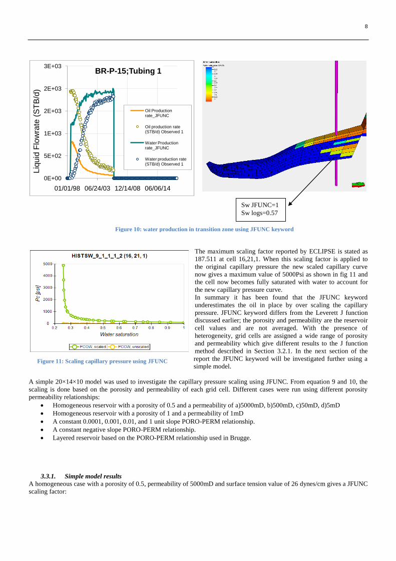
The shift in the oil water contact causes most cells near the bottom of the reservoir to become fully saturated with water,

therefore decreasing oil production. The result for Producer 15 with JFUNC is shown in fig 10. It can be seen that the well has

more water initially and so produces less oil than expected. For the completion cell at a depth of 5447ft the water saturation is

1.0 which no longer agrees with the logs.

Figure 8: Impact of using JFUNC keyword on the oil production rate and the recovery

Figure 9: Impact of using JFUNC keyword on the water production

8

Sw JFUNC=1

Sw logs=0.57

0E+00

5E+02

1E+03

2E+03

2E+03

3E+03

01/01/98 06/24/03 12/14/08 06/06/14

Liq

uid

Flo

wra

te (

ST

B/d

)

BR-P-15;Tubing 1

Oil Production rate_JFUNC

Oil production rate (STB/d) Observed 1

Water Production rate_JFUNC

Water production rate (STB/d) Observed 1

The maximum scaling factor reported by ECLIPSE is stated as

187.511 at cell 16,21,1. When this scaling factor is applied to

the original capillary pressure the new scaled capillary curve

now gives a maximum value of 5000Psi as shown in fig 11 and

the cell now becomes fully saturated with water to account for

the new capillary pressure curve.

In summary it has been found that the JFUNC keyword

underestimates the oil in place by over scaling the capillary

pressure. JFUNC keyword differs from the Leverett J function

discussed earlier; the porosity and permeability are the reservoir

cell values and are not averaged. With the presence of

heterogeneity, grid cells are assigned a wide range of porosity

and permeability which give different results to the J function

method described in Section 3.2.1. In the next section of the

report the JFUNC keyword will be investigated further using a

simple model.

A simple 20×14×10 model was used to investigate the capillary pressure scaling using JFUNC. From equation 9 and 10, the

scaling is done based on the porosity and permeability of each grid cell. Different cases were run using different porosity

permeability relationships:

Homogeneous reservoir with a porosity of 0.5 and a permeability of a)5000mD, b)500mD, c)50mD, d)5mD

Homogeneous reservoir with a porosity of 1 and a permeability of 1mD

A constant 0.0001, 0.001, 0.01, and 1 unit slope PORO-PERM relationship.

A constant negative slope PORO-PERM relationship.

Layered reservoir based on the PORO-PERM relationship used in Brugge.

3.3.1. Simple model results

A homogeneous case with a porosity of 0.5, permeability of 5000mD and surface tension value of 26 dynes/cm gives a JFUNC

scaling factor:

Figure 10: water production in transition zone using JFUNC keyword

Figure 11: Scaling capillary pressure using JFUNC

9

This is the multiplier that is applied to the capillary pressure values in the SWOF table. The water saturations are slightly

higher in each cell and the top of the transition zone is shifted up by one layer. Table 2shows the initial water distribution with

the JFUNC switch on and off. The critical water saturation is 0.252. From the table it is clear that the water is mobile at a

higher level in the reservoir with JFUNC activated. When the ratio of porosity and permeability becomes larger the scaling

factor increases and therefore the scaled capillary pressure increases, increasing the initial water saturation distribution. When

the ratio is 0.01, the oil water contact shifts up by one layer, when the ratio is 0.1 it shifts up by 3 layers and when the ratio is 1

the reservoir becomes fully saturated with water, in comparison to the original distribution based on the relative permeability

curves as shown in table 2. Constant slopes of 0.0001, 0.001, 0.01, 0.1, and 1 give the same ratios of porosity/permeability at

each grid cell as those gained from the homogeneous reservoirs.

The oil production rate when the JFUNC is switched on decreases for each case and the water production increases with the

same water breakthrough. The oil and water production rates for each case are shown in appendix (59-84). The oil recovery

efficiency consistently decreases as the ratio increases, the recovery factors are plotted for all cases in table 3

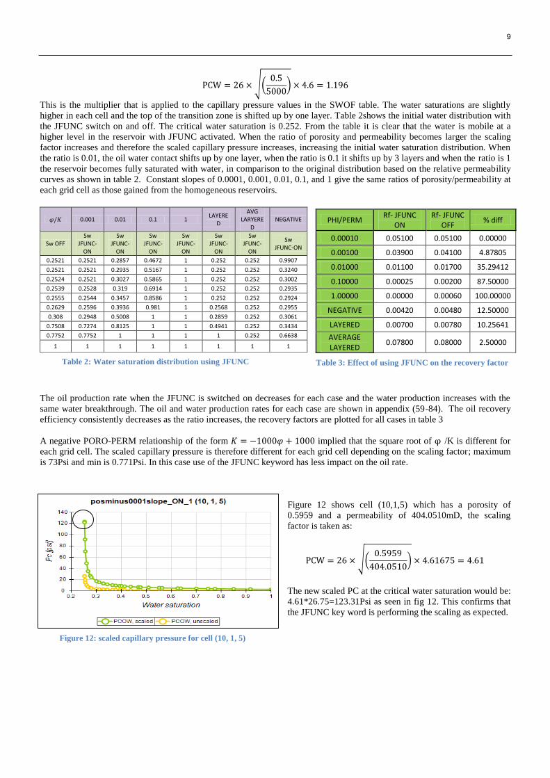
A negative PORO-PERM relationship of the form implied that the square root of /K is different for

each grid cell. The scaled capillary pressure is therefore different for each grid cell depending on the scaling factor; maximum

is 73Psi and min is 0.771Psi. In this case use of the JFUNC keyword has less impact on the oil rate.

Figure 12 shows cell (10,1,5) which has a porosity of

0.5959 and a permeability of 404.0510mD, the scaling

factor is taken as:

The new scaled PC at the critical water saturation would be:

4.61*26.75=123.31Psi as seen in fig 12. This confirms that

the JFUNC key word is performing the scaling as expected.

PHI/PERM Rf- JFUNC

ON Rf- JFUNC

OFF % diff

0.00010 0.05100 0.05100 0.00000

0.00100 0.03900 0.04100 4.87805

0.01000 0.01100 0.01700 35.29412

0.10000 0.00025 0.00200 87.50000

1.00000 0.00000 0.00060 100.00000

NEGATIVE 0.00420 0.00480 12.50000

LAYERED 0.00700 0.00780 10.25641

AVERAGE LAYERED

0.07800 0.08000 2.50000

0.001 0.01 0.1 1 LAYERE

D

AVG LARYERE

D NEGATIVE

Sw OFF Sw

JFUNC-ON

Sw JFUNC-

ON

Sw JFUNC-

ON

Sw JFUNC-

ON

Sw JFUNC-

ON

Sw JFUNC-

ON

Sw JFUNC-ON

0.2521 0.2521 0.2857 0.4672 1 0.252 0.252 0.9907

0.2521 0.2521 0.2935 0.5167 1 0.252 0.252 0.3240

0.2524 0.2521 0.3027 0.5865 1 0.252 0.252 0.3002

0.2539 0.2528 0.319 0.6914 1 0.252 0.252 0.2935

0.2555 0.2544 0.3457 0.8586 1 0.252 0.252 0.2924

0.2629 0.2596 0.3936 0.981 1 0.2568 0.252 0.2955

0.308 0.2948 0.5008 1 1 0.2859 0.252 0.3061

0.7508 0.7274 0.8125 1 1 0.4941 0.252 0.3434

0.7752 0.7752 1 1 1 1 0.252 0.6638

1 1 1 1 1 1 1 1

Table 2: Water saturation distribution using JFUNC Table 3: Effect of using JFUNC on the recovery factor

Figure 12: scaled capillary pressure for cell (10, 1, 5)

10

So far a simple linear relationship has been used to describe the relationship between porosity and permeability. It is common

practice to use a PORO-PERM relationship that is described by a log relationship.

A layered reservoir has been tested with the JFUNC using a PORO-PERM

relationship of the following form:

The porosities and permeabilities used for each layer are outlined in table. As

discussed earlier each layer will have a corresponding ratio of /K and

therefore a different scaling factor. Table 4 shows the maximum capillary

pressure values for each layer, which vary between 1.16 and 530.97. The

production rate is underestimated using JFUNC and the water production is

consistently overestimated in each case (see Appendix fig 60-91)

An average value of porosity and permeability was used which gave an

unreliable scaling with High CPU time and convergence problems see fig88-

89-Appendix.

From the results discussed above, using a JFUNC keyword causes the volume of hydrocarbon in place to decrease as the ratio

of porosity and permeability increases. The recovery factor is defined as the volume of oil produced/volume of oil initially in

place. So why does the recovery factor vary when the JFUNC is used? Capillary pressure is scaled up and the corresponding

water saturation value increases. This results in much higher mobility for water, reduced mobility for the oil and higher water

cut at the production wells.

3.4. Initial water distribution using SWCR and SWL

Initial water distribution can be defined using SWL specifying the connate water saturation for each cell and the SWCR

specifying the critical water saturation for each cell. The relative permeability/capillary pressures are then scaled accordingly.

A common problem that reservoir engineers face when initializing a model is the control of water breakthrough in transition

zones. In most cases where a well has been completed above the oil water contact water free production is expected for the

early production period. In many cases the SWCR/SWL keywords are used to scale Kr curves to achieve the expected

behavior.

In order to control water movement in the transition zone, SWCR is set to the initial water saturation distribution. Water

saturation is described using the equation:

Equation 11

Setting SWCR to the initial water implies that the reservoir has no dynamic range and the water is immobile.

Several cases have been run to investigate the impact on controlling the water breakthrough using such keywords and weather

the stability of the model is affected. The CPU time is recorded and compared for all cases and the equilibrium state is

investigated.

Cases Performed include:

1. SWL=SWCR=SWATINIT array

2. SWL=SWCR+0.01=SWATINIT array

3. SWL=SWCR=SWATINIT, PC=0

4. a)SWL=Sw randomly distributed=SWATINIT b)SWATINIT=Sw randomly distributed

When SWCR is set to the initial water distribution, there are conditions that should be satisfied for the simulation to run:

SWCR≥SWL for each grid cell, critical oil saturation (1-SW) ≤critical oil saturation from SWOF table, and no major

convergence problems present.

Setting SWL=SWCR=SWATINIT meant that some cells have a water saturation of 1, causing a consistency problem with the

oil phase end points in some grid cells, as the critical oil saturation is greater than zero.. This also causes simulation

convergence problems. When the model was checked by running with no wells for thirty days, fluids were displaced, showing

that it was not initially in equilibrium. Fig15 shows the oil production rate match which was far from the observed data.

In the following case, the highest critical water saturation is 0.252, therefore the SWL=SWCR has been clipped to a value of

0.74 so that the maximum oil phase end point of 1-0.252 is taken into account. This gives a STOIIP of 775MBbl. Although

this has prevented inconsistencies, there were still some convergence problems.

PERM POR maximum capillary pressure

1.8152 0.05 530.97

9.1427 0.1 334.59

46.0492 0.15 182.59

231.936 0.2 93.94

1168.19 0.25 46.80

5883.81 0.3 22.84

29634.9 0.35 10.99

14926 0.4 16.56

751787 0.45 2.47

3.78E+06 0.5 1.16

Table 4: PCW values for JFUNC based on a

PORO-PERM

11

0

5000

10000

15000

20000

25000

30000

35000

40000

45000

01/01/98 06/24/03 12/14/08 06/06/14

Liq

uid

Flo

wra

te (

ST

B/d

)


SWL=SWCR=SWATINIT capped at 0.74

Lambda

Observed 1

0

5000

10000

15000

20000

25000

30000

01/01/98 06/24/03 12/14/08 06/06/14

Liq

uid

Flo

wra

te (

ST

B/d

)Field Water production rate

SWL=SWCR=SWATINIT capped ot 0.74

Lambda

Observed 1

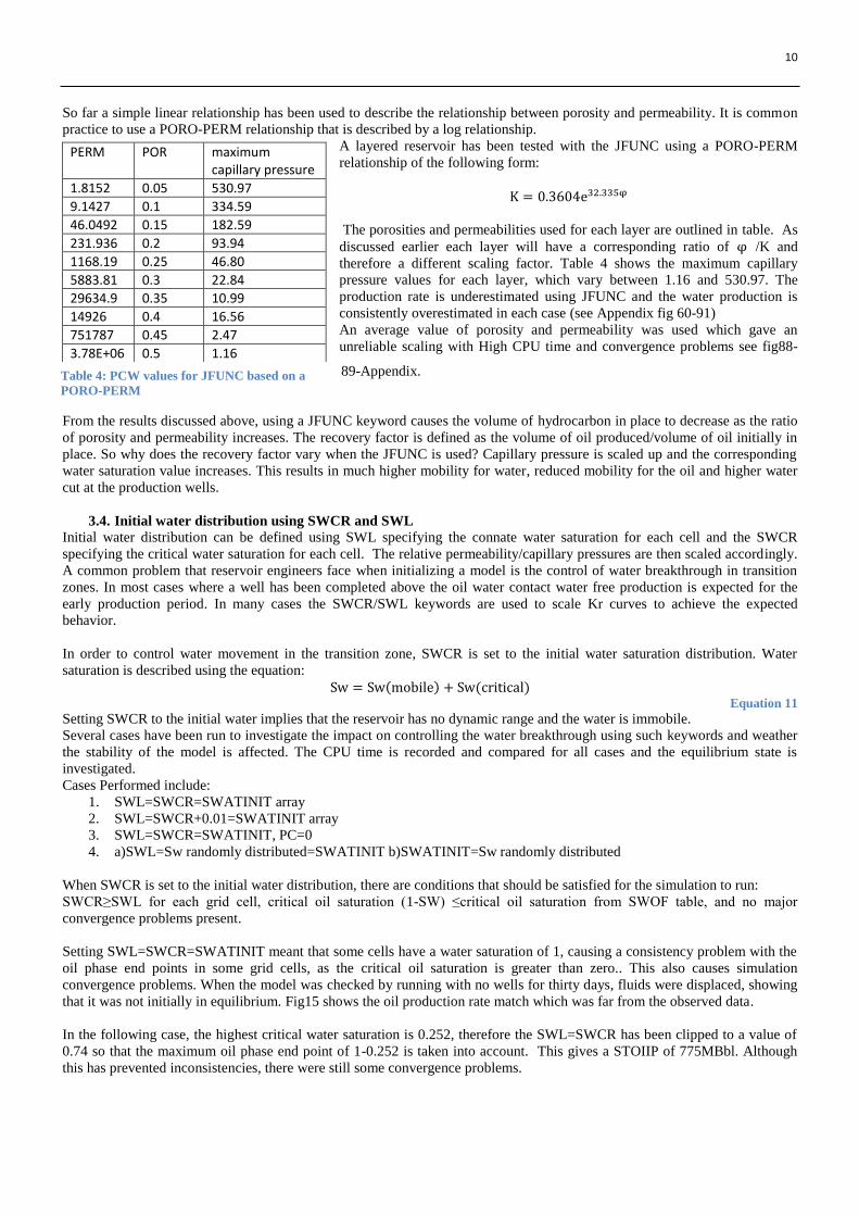
Fig 14 shows the scaling for cell (61,1,9). The initial

SWCR on the Krw curve is 0.3, but is now scaled to 0.74.,

As this value also corresponds to the connate water

saturation, the water is never mobile. Fig 15 shows the oil

and water production profiles in comparison to the

observed data. Although the water breakthrough was

delayed, it matched the oil production profile for the first

year giving water free oil production and producing water

one year later than expected. The water production is then

greatly underestimated as shown in fig 15. , the oil

production rate is overestimated and the production history

is mismatched in comparison to Lambda function.

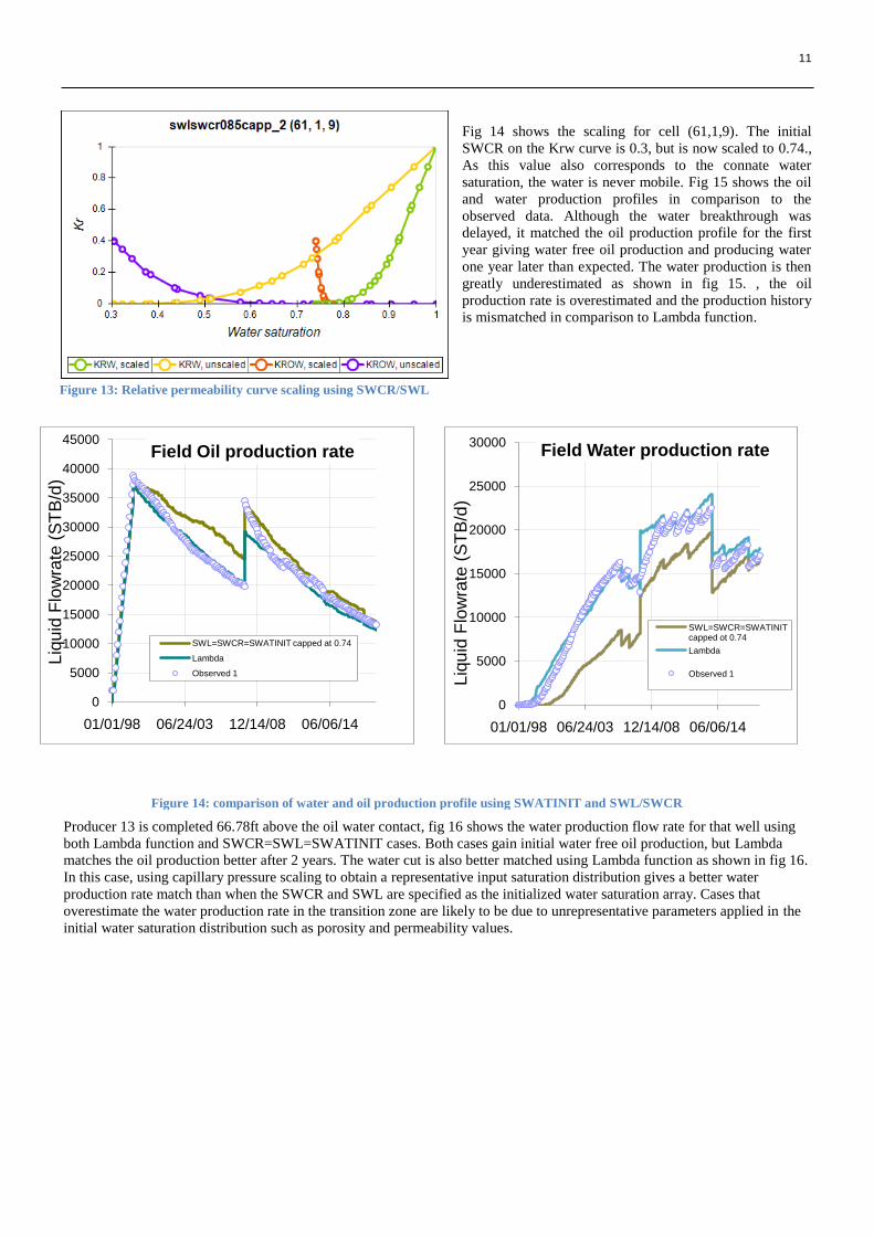
Producer 13 is completed 66.78ft above the oil water contact, fig 16 shows the water production flow rate for that well using

both Lambda function and SWCR=SWL=SWATINIT cases. Both cases gain initial water free oil production, but Lambda

matches the oil production better after 2 years. The water cut is also better matched using Lambda function as shown in fig 16.

In this case, using capillary pressure scaling to obtain a representative input saturation distribution gives a better water

production rate match than when the SWCR and SWL are specified as the initialized water saturation array. Cases that

overestimate the water production rate in the transition zone are likely to be due to unrepresentative parameters applied in the

initial water saturation distribution such as porosity and permeability values.

Figure 13: Relative permeability curve scaling using SWCR/SWL

Figure 14: comparison of water and oil production profile using SWATINIT and SWL/SWCR

12

0

0.1

0.2

0.3

0.4

0.5

0.6

0.7

01/01/98 06/24/03 12/14/08 06/06/14

Liq

uid

To

Liq

uid

Ratio

(ST

B/S

TB

)

Field Water cut

SWL=SWCR=SWATINIT capped at 0.74

Lambda

Observed 1

0

500

1000

1500

2000

2500

3000

01/01/98 06/24/03 12/14/08 06/06/14

Liq

uid

Flo

wra

te (

ST

B/d

)

BR-P-13;Tubing 1 Water production rate

SWL=SWCR=SWATINIT capped at 0.74Lambda

Observed 1

0

5000

10000

15000

20000

25000

30000

35000

40000

45000

01/01/98 06/24/03 12/14/08 06/06/14

Liq

uid

Flo

wra

te (

ST

B/d

)



Observed 1

0

5000

10000

15000

20000

25000

30000

1/1/98 6/24/03 12/14/08 6/6/14

Liq

uid

Flo

wra

te (

ST

B/d

)



Observed 1

SWL=SWCR=SWATINI_0Pc

Case SWATINIT=SWCR=SWL took longer than the Lambda function but was still in equilibrium. The recovery efficiency of

case 1 and Lambda case are 23% and 21% respectively.

When SWL=SWCR+0.1=SWATINIT clipped to a maximum value of 0.74 was run, the results were exactly the same as the

previous case but the run took less time to converge. The CPU time is recorded for each case in table 8 in the appendix

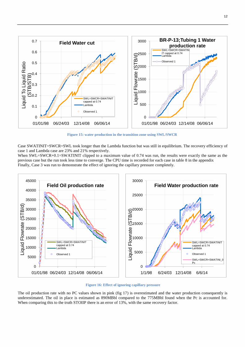
Finally, Case 3 was run to demonstrate the effect of ignoring the capillary pressure completely.

The oil production rate with no PC values shown in pink (fig 17) is overestimated and the water production consequently is

underestimated. The oil in place is estimated as 890MBbl compared to the 775MBbl found when the Pc is accounted for.

When comparing this to the truth STOIIP there is an error of 13%, with the same recovery factor.

Figure 15: water production in the transition zone using SWL/SWCR

Figure 16: Effect of ignoring capillary pressure

13

0

5000

10000

15000

20000

25000

30000

35000

40000

45000

1/1/98 6/24/03 12/14/08 6/6/14

Liq

uid

Flo

wra

te (

ST

B/d

)

Field Oil production rateObserved 1

ransom SWATINIT distribution

random SWCR=SWL=SWATINIT distribution

0

5000

10000

15000

20000

25000

30000

35000

40000

45000

50000

01/01/98 06/24/03 12/14/08 06/06/14L

iqu

id F

low

rate

(S

TB

/d)


Observed 1

SWATINIT random distribution

SWL=SWCR=SWATINIT random distribution

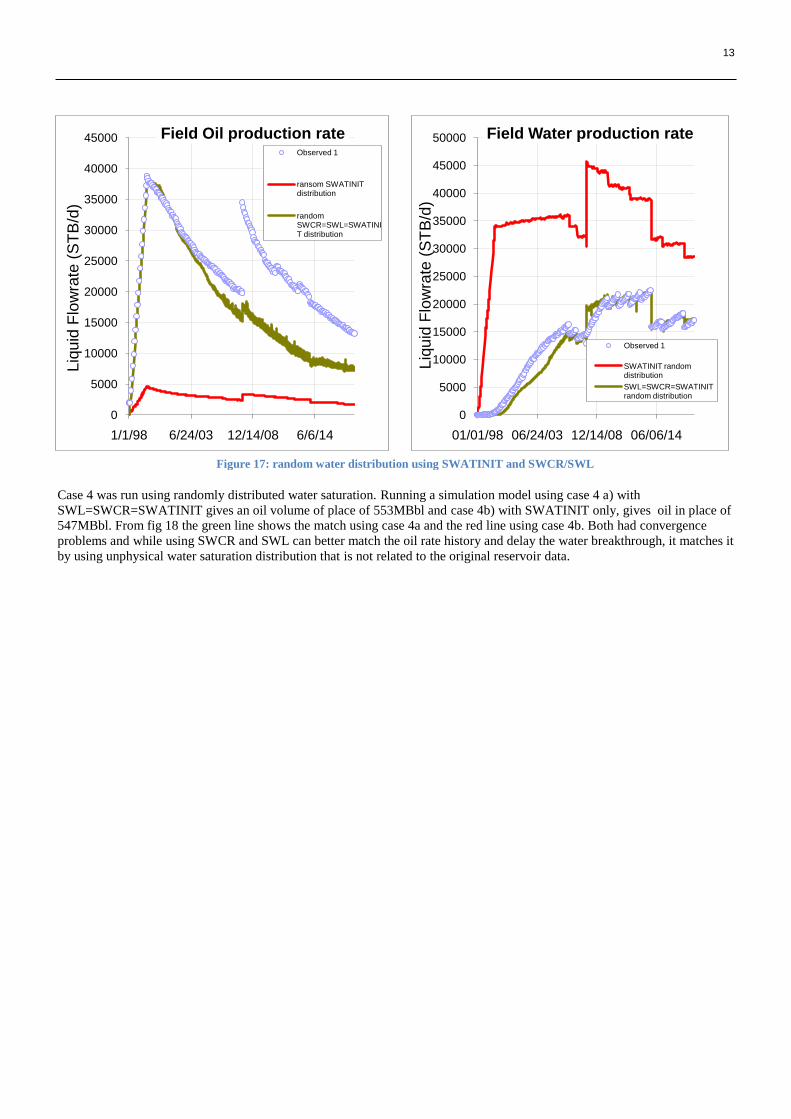
Case 4 was run using randomly distributed water saturation. Running a simulation model using case 4 a) with

SWL=SWCR=SWATINIT gives an oil volume of place of 553MBbl and case 4b) with SWATINIT only, gives oil in place of

547MBbl. From fig 18 the green line shows the match using case 4a and the red line using case 4b. Both had convergence

problems and while using SWCR and SWL can better match the oil rate history and delay the water breakthrough, it matches it

by using unphysical water saturation distribution that is not related to the original reservoir data.

Figure 17: random water distribution using SWATINIT and SWCR/SWL

14

4. Discussion The problem of initializing a simulation model using a representative water saturation distribution is becoming widely

recognized. The Middle East has two thirds of all recoverable oil in the world. With most Middle Eastern reservoirs being

largely extensive carbonates and low permeable sandstone, the capillary pressure plays an important role in water saturation

modeling. Shehadeh (Shehadeh K. Masalmeh 2000) attempts to describe the mobility of oil in the transition zone and relates it

to the initial oil saturation distribution. It is found that as the initial oil saturation gets close to the residual, the mobility

increases. This implies that the mobility of oil in the transition zone is possibly higher than anywhere else in the reservoir. This

paper however did not explain how the saturations can be estimated accurately and utilized in the computer model. Many

papers have been published on the water saturation heights and their impact on the hydrocarbon in place such as Harrison

(B.Harrison 2001) and Wiltgen (Nick A. Wiltgen 2003) which compares the saturation heights predicted water saturations

against the log water saturations. Harrison (B.Harrison 2001)predicts that Cuddy’s log based method is the simplest most

effective method to use; Wiltgen (Nick A. Wiltgen 2003) concludes that the Skelt and Harrison method gave the best result

and using this project as an example, Lambda function gave the best estimates. Whilst all these findings may be contradictory,

it shows that each oil field is different, with many different reservoir features and behavior. This project therefore highlights

the differences in using those methods and does not necessarily recommend a specific method to be used. Those papers

mentioned investigate the best method to be used in terms of matching the logs water saturation, none of them however look at

the effects of scaling capillary pressure using the methods described and implementing them in the simulator which this

project does using the SWATINIT keyword.

Al Junaibi (Faisal Al Jenaibi 2008) addresses the importance of using dynamic rock typing where the reservoir is split into

regions according to the irreducible water saturation taken from logs and an equation relating the FWL to the irreducible water

saturation using two constants. The log water saturation vs. height above free water level sometimes gives a very weak

correlation and so correlation using porosity and permeability may be a better option as some of the water saturation height

methods provide.

Rojas (Rojas 2010) describes the application of J-Function to prepare a consistent tight gas reservoir simulation model. This

paper proposes inputting a J function keyword which calculates Sw according to the porosity and permeability. The conclusion

of this paper is that the “J function technique has proven to be a very powerful tool to accurately to distribute fluids in a tight

gas reservoir” it is claimed that the technique honours the capillary forces, permeability and porosity and shows that the

volume in place is representative providing a good history match. This is an interesting finding which is different from the

outcome of using JFUNC keyword in this report. This again could be due to a difference in the reservoir but could also be an

interesting area of further investigation. It could be that the JFUNC works better for gas than oil reservoirs.

Eigstead (Geir Terje Eigestd 2000) Investigates the capillary pressure in the transition zones using a hysteresis model but did

not apply it to a case where a match could be compared in a layered reservoir. Hysteresis is an important aspect of the fluid

distribution in the transition zone. In this project like many others only drainage is taken into account and the simulation is

performed accordingly. The discussion raised recently in the SPE TIG (SPE 2011) clearly reflects the many different opinions

about initializing models, to correctly describe an initial water distribution that best predicts later fluid production. The type of

problem that many engineers face is when water breakthrough occurs after a few months, with no evidence from relative

permeability curves or logs to explain what is happening. In the discussion it was suggested that, by setting the critical water

saturation and the connate water saturation equal to the initial water saturation distribution given by the geologist, the

simulation would be initialized correctly. However this approach does not generally give representative dynamic behavior and

the match is not accurate as seen in the previous section 3.4.

5. Conclusion The case study using the SPE Brugge model demonstrates how the choice of capillary pressure model can significantly affect

the simulation results. The use of a simplified test example can help to explain how the different simulation options work.

The main findings of this project include:

Representative capillary pressure curves are a key to accurately predicting the process of oil recovery and describing

the fluid distribution

Based on the results obtained, the Lambda function gave a better match to the Brugge case in terms of fluids in place

and the maximum scaled capillary pressure

The JFUNC keyword results in different scaling for every grid cell and causes the volume of fluids in place to

decrease as the ratio of porosity and permeability increases

Setting SWCR=SWL=SWATINIT causes consistency errors, and even when limited to a maximum critical

saturation, convergence problems persist, dynamic behavior is restricted and the oil rate is overestimated

6. Recommendation It is recommended that the approach taken in this report is followed and sensitivity analysis is performed on the capillary

pressure as well as other parameters when a good history match is required. This work could be further developed when a

three phase model is present; investigating the effectiveness of the keywords when a gas cap is present. This report

concentrated on drainage only and so further work on the effect of hysteresis could be done.

15

Nomenclature

Symbol Description Units

A,B,C and D Regression Constants None

J J function Dimensionless

K Permeability mD

Pc Capillary Pressure Psi

Pcm Maximum Capillary pressure from SWOF table Psi

Pct Capillary Pressure from SWOF table Psi

PCW Maximum Scaled Capillary Pressure Psi

PCOW Simulator Oil Water Capillary Pressure Psi

Sw Water Saturation None

Swirr Irreducible Water Saturation None

Swn Normalized Water Saturation None

a, b and c Constants None

d Pore Diameter Ft

g Gravity acceleration Ft2/sec

h Height above free water level Ft

λ Regression constant None

φ Porosity None

Density of oil Lb/ft3

Density of water Lb/ft3

θ Contact angle degrees

16

7. References

Cuddy, Steve. "A SImple Convincing Model For Calculating Water Saturations In Southern North Sea Gas Fields." SPWLA

34th Annual Logging Sypnosium, 1993.

A Rojas, ConcoPhillips. "Application of J-Function to Prepare a Consistent Tight Gas Reservoir Simulation Model: Bossier

Field." SPE138412, 2010.

Adel Ibrahim, Zaki Bassiouni, and Robert Desbrandes. "Determination of Relative Permeability Curves in Tight Gas Sands

using Log Data." SPWLA 33rd Annual Logging Symposium, 1992.

B.Harrison, X.D.Jing. "Saturation Height Methods and Their Impact on Volumetric Hydrocarbon in Place Estimates."

SPE71326, 2001.

E. Peters, R.J. Arts, and G.K.Brouwer and C.R.Geel. "Results of the Brugge Benchmark Study for Flooding Optimization and

History matching." SPE 119094, 2009.

E.Peters, TNO. "Results of the Brugge Benchmark Study for Flooding Optimization and History Matching." SPE119094,

2009.

Faisal Al Jenaibi, Khalid Hammadi, Lutfi Salameh, Abu Dhabi National Oil Company. "New Methodology for Optimized

Field Development Plan, Why Do We Need TO Introduce Dynamic Rock Typing." SPE 117894, 2008.

Geir Terje Eigestd, University of Bergen, Norway and Johne Alex Larsen, Norsk Hydro Research Center, Norway.

"Numerical Modelling of Capillary Tranzition Zone." SPE64374, 2000.

Harrison, Christopher Skelt and Bob. "An Integrated Approach to Saturation Height Analysis." SPWLA 36th annual Logging

Sypnosium, 1995.

Holmes, Michael. "Capillary Pressure & Relative Permeability Petrophysical Reservoir Models." Digital Formation. May

2002. http://www.digitalformation.com/Documents/CPRP.pdf (accessed 07 2011).

Johnson, A. "Permeability Averaged Capillary Data." SPWLA 28th Annual Logging Symposium, 1992.

M.C.Leverette. "Capillary Behaviour in Porous Solids." Transaction of the AIME(142), 1941.

Nick A. Wiltgen, Joel Le Calvez, and Keith Owen, Schlumberger. "Methods Of Saturation Modelling Using Capillary

Pressure Averaging and Pseudos." SPWLA 44th Annual Logging Symposium, 2003.

Shehadeh K. Masalmeh, Shell Technology Exploration and Production Rijswik, The Netherlands. "High Oil Recoveriesfrom

tranzition zones." SPE 87291, 2000.

SPE. Reservoir Simulation Discussion Forum/ Mobile Water and tranzition zones. 06 28, 2011.

http://communities.spe.org/TIGS/SIM/Lists/Team%20Discussion (accessed 06 28, 2011).

Y.Wang, SPE,Schlumberger, and Petronas and M.Z.Sakdilah M.Bandal. "Asystematc Approch to incorporate Capillary

Pressure Saturation Data into Reservoir Simulation." SPE101013, 2006.

17

Appendix

SPE/SPWLA

No

Year Title Authors Conclusions

SPE 941152 1941 Capillary behavior in

Porous Solids

M.C.Leverett Multiple curves can be converted into

a single universal curve using the J

function.

SPE 5126 1975 The Effect of Capillary

Pressure in a Multilayer

Model of Porous Media

R.G.Hawthorne Equations developed to describe

immiscible fluid displacement in a

multichannel model when capillary

pressure affects the crossflow between

channels.

SPE 8234 1981 A Simple Correlation

Between Permeabilities and

Mercury Capillary

Pressures

B.F Swanson Direct measurement of brine

permeability of clean sands from

capillary pressure plot data. New

correlation is developed to improve

measurements on drill cuttings and

sidewall core samples

SPWLA 28th

1987 Permeability averaged

Capillary Data

A Johnson Log Sw=AlogK+B. permeability

averaged capillary analysis. Does not

rely on any profound theoretical basis.

SPWLA 36th

1995 An integrated approach to

saturation height analysis

Christopher Skelt and

Bob Harrison

Added a weighting function to give a

better fit to capillary pressure data

SPWLA 44th

2003 Methods Of Saturation

Modelling using capillary

pressure Averaging and

Pseudos

Nick.AWiltgen, Joel le

Calvez and Keith Owen

Lambda function similar to Skelt and

Harrison and Leverett is used to fit

capillary pressure data by applying a

constant called λ.

18

0.E+00

5.E+03

1.E+04

2.E+04

2.E+04

3.E+04

3.E+04

4.E+04

4.E+04

5.E+04

1/1/98 9/27/00 6/24/03 3/20/06 12/14/08 9/10/11 6/6/14 3/2/17

Liq

uid

Flo

wra

te (

ST

B/d

)


Observed 1 case 2-EQUIL Case1-EQUILCase9-EQUIL Case40-EQUIL Case11-EQUILCase49-EQUIL Case80-EQUIL Case84-EUILCase91-EQUIL

0.E+00

5.E+03

1.E+04

2.E+04

2.E+04

3.E+04

3.E+04

01/01/98 09/27/00 06/24/03 03/20/06 12/14/08 09/10/11 06/06/14 03/02/17

Liq

uid

Flo

wra

te (

ST

B/d

)


Case2-EQUIL Case1-EQUIL Case9-EQUILCase40-EQUIL Case11-EQUIL Case49-EQUILCase80-EQUIL Case84-EQUIL Case91-EQUILObserved 1

EQUIL

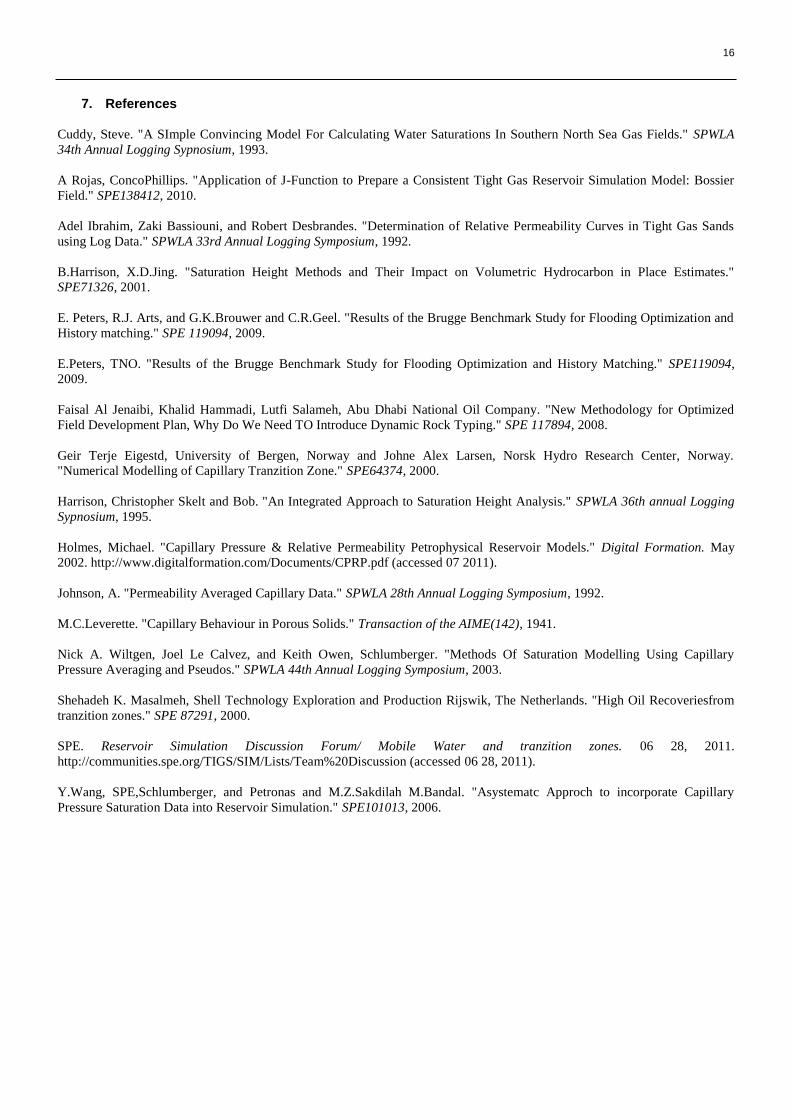
Figure 18: 10 best cases showing the field oil production rate using EQUIL with case 9 giving the closest match

Figure 19:10 best cases showing the field water production rate using EQUIL with case 9 giving the closest match

19

0.E+00

2.E+07

4.E+07

6.E+07

8.E+07

1.E+08

1.E+08

1.E+08

2.E+08

2.E+08

2.E+08

1/1/98 9/27/00 6/24/03 3/20/06 12/14/08 9/10/11 6/6/14 3/2/17

Liq

uid

Pro

du

cti

on

Vo

lum

e (

ST

B)

Field Oil production cumulative

Case2-EQUIL Case1-EQUILCase9-EQUIL Case40-EQUILCase11-EQUIL Case49-EQUILCase80-EQUIL Case84-EQUILCase91-EQUIL Observed 1

0.E+00

2.E+07

4.E+07

6.E+07

8.E+07

1.E+08

1.E+08

1/1/98 9/27/00 6/24/03 3/20/06 12/14/08 9/10/11 6/6/14 3/2/17

Liq

uid

Pro

du

cti

on

Vo

lum

e (

ST

B)

Field Water production cumulative

Case2-EQUIL Case1-EQUIL




Case91-EQUIL Observed 1

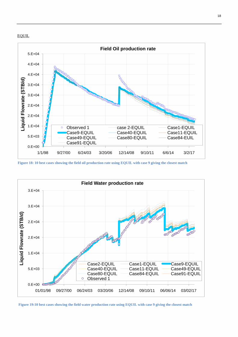
Figure 21: 10 best cases showing the field water cumulative production using EQUIL with case 9 giving the closest match

Figure 20: 10 best cases showing the field oil cumulative production using EQUIL with case 9 giving the closest match

20

0.E+00

5.E+03

1.E+04

2.E+04

2.E+04

3.E+04

3.E+04

4.E+04

4.E+04

5.E+04

01/01/98 09/27/00 06/24/03 03/20/06 12/14/08 09/10/11 06/06/14 03/02/17

Liq

uid

Flo

wra

te (

ST

B/d

)


Observed 1 91-JFunction 80-JFunction 49-JFunction

40-JFunction 11-JFunction 9-JFunction

0.E+00

5.E+03

1.E+04

2.E+04

2.E+04

3.E+04

3.E+04

01/01/98 09/27/00 06/24/03 03/20/06 12/14/08 09/10/11 06/06/14 03/02/17

Liq

uid

Flo

wra

te (

ST

B/d

)


Observed 1 91-JFunction 80-JFunction

49-JFUnction 40-JFunction 11-JFUnction

9-JFunction

SWATINIT

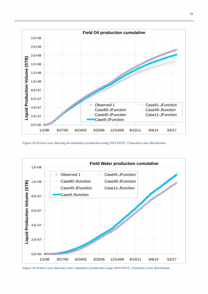
1. J-Function

Figure 23:10 best cases showing field water production rate using STAWTINIT, J function water distribution

Figure 22:10 best cases showing oil production rate using SWATINIT, J function water distribution

21

0.E+00

2.E+07

4.E+07

6.E+07

8.E+07

1.E+08

1.E+08

1.E+08

2.E+08

2.E+08

2.E+08

1/1/98 9/27/00 6/24/03 3/20/06 12/14/08 9/10/11 6/6/14 3/2/17

Liq

uid

Pro

du

cti

on

Vo

lum

e (

ST

B)


Observed 1 Case91-JFunction

Case80-JFunction Case49-Jfunction

Case40-JFunction Case11-JFunction

Case9-JFunction

0.E+00

2.E+07

4.E+07

6.E+07

8.E+07

1.E+08

1.E+08

1/1/98 9/27/00 6/24/03 3/20/06 12/14/08 9/10/11 6/6/14 3/2/17

Liq

uid

Pro

du

cti

on

Vo

lum

e (

ST

B)


Observed 1 Case91-JFunction

Case80-Jfunction Case49-JFunction

Case40-JFunction Case11-Jfunction

Case9-Jfunction

Figure 25:10 best cases showing water cumulative production using SWATINIT, J function water distribution

Figure 24:10 best cases showing oil cumulative production using SWATINIT, J function water distribution

22

0.E+00

5.E+03

1.E+04

2.E+04

2.E+04

3.E+04

3.E+04

4.E+04

4.E+04

5.E+04

01/01/98 09/27/00 06/24/03 03/20/06 12/14/08 09/10/11 06/06/14 03/02/17

Liq

uid

Flo

wra

te (

ST

B/d

)


Observed 1Case9-Skelt and HarrisonCase2-Skelt and HarrisonCase11-Skelt and HarrisonCase40-Skelt and HarrisonCase49-Skelt and HarrisonCase80-Skelt and HarrisonCase84-Skelt and HarrisonCase91-Skelt and HarrisonCase1-Skelt and Harrison

0

5000

10000

15000

20000

25000

30000

01/01/98 09/27/00 06/24/03 03/20/06 12/14/08 09/10/11 06/06/14 03/02/17

Liq

uid

Flo

wra

te (

ST

B/d

)


Observed 1Case9-Skelt and HarrisonCase2-Skelt and HarrisonCase11-Skelt and HarrisonCase40-Skelt and HarrisonCase49-Skelt and HarrisonCase80-Skelt and HarrisonCase84-Skelt and HarrisonCase91-Skelt and HarrisonCase1-Skelt and Harrison

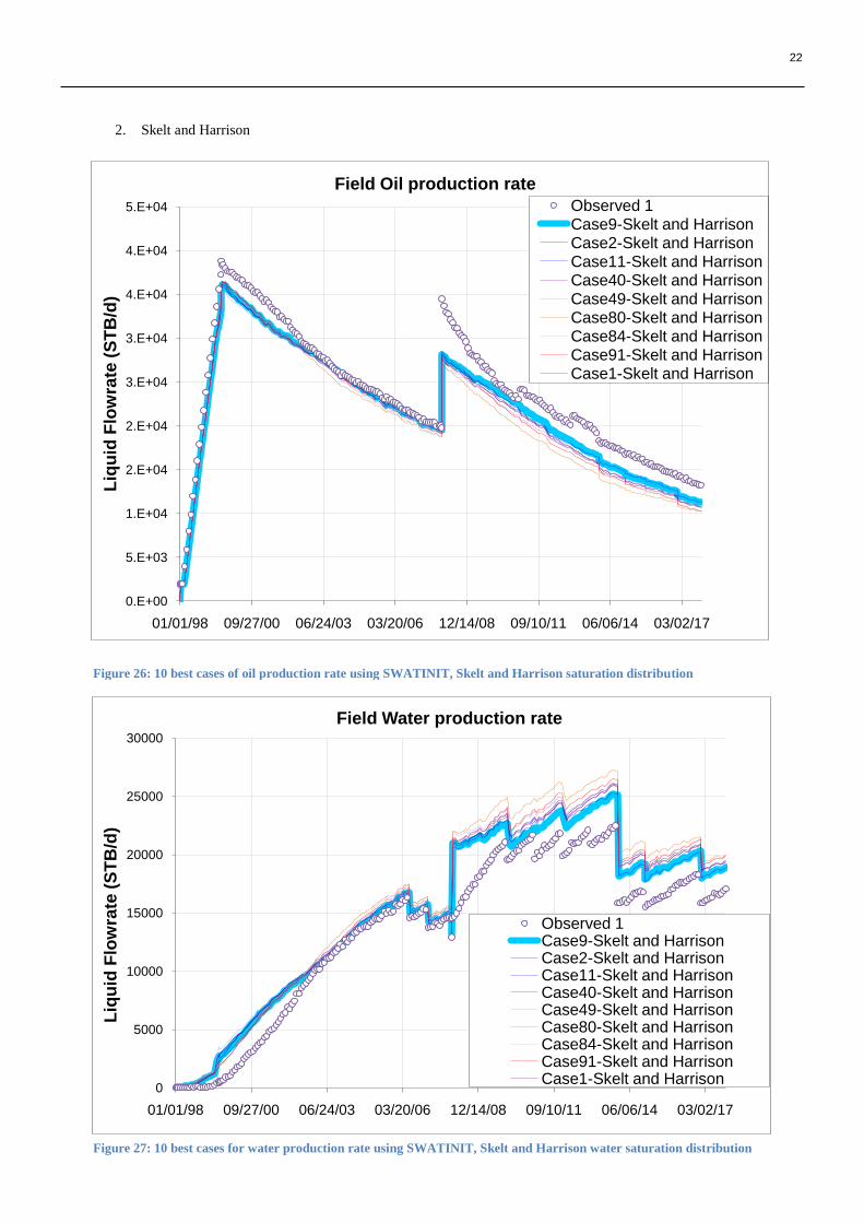
2. Skelt and Harrison

Figure 26: 10 best cases of oil production rate using SWATINIT, Skelt and Harrison saturation distribution

Figure 27: 10 best cases for water production rate using SWATINIT, Skelt and Harrison water saturation distribution

23

0.E+00

2.E+07

4.E+07

6.E+07

8.E+07

1.E+08

1.E+08

1.E+08

2.E+08

2.E+08

2.E+08

01/01/98 09/27/00 06/24/03 03/20/06 12/14/08 09/10/11 06/06/14 03/02/17

Liq

uid

Pro

du

cti

on

Vo

lum

e (

ST

B)


Observed 1Case9-Skelt and HarrisonCase2-Skelt and HarrisonCase11-Skelt and HarrisonCase40-Skelt and HarrisonCase49-Skelt and HarrisonCase80-Skelt and HarrisonCase84-Skelt and HarrisonCase91-Skelt and Harrison

0.E+00

2.E+07

4.E+07

6.E+07

8.E+07

1.E+08

1.E+08

1.E+08

01/01/98 09/27/00 06/24/03 03/20/06 12/14/08 09/10/11 06/06/14 03/02/17

Liq

uid

Pro

du

cti

on

Vo

lum

e (

ST

B)


Observed 1

Case9-Skelt and Harrison









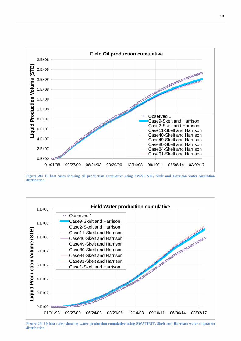
Figure 28: 10 best cases showing oil production cumulative using SWATINIT, Skelt and Harrison water saturation

distribution

Figure 29: 10 best cases showing water production cumulative using SWATINIT, Skelt and Harrison water saturation

distribution

24

0.E+00

5.E+03

1.E+04

2.E+04

2.E+04

3.E+04

3.E+04

4.E+04

4.E+04

5.E+04

1/1/98 9/27/00 6/24/03 3/20/06 12/14/08 9/10/11 6/6/14 3/2/17

Liq

uid

Flo

wra

te (

ST

B/d

)


Observed 1 Case9-Lambda Case2-Lambda

Case11-Lambda Case40-Lambda Case49-Lambda

Case80-Lambda Case84-Lambda Case91-lambda

0.E+00

5.E+03

1.E+04

2.E+04

2.E+04

3.E+04

3.E+04

01/01/98 27/09/00 24/06/03 20/03/06 14/12/08 10/09/11 06/06/14 02/03/17

Liq

uid

Flo

wra

te (

ST

B/d

)


Observed 1 Case2-Lambda

Case9-Lambda Case11-Lambda



Case91-Lambda

3. Lambda

Figure 31: 10 best cases showing oil production rate using SWATINIT, Lambda water saturation distribution

Figure 30: 10 best cases showing water production rate using SWATINIT, Lambda water saturation distribution

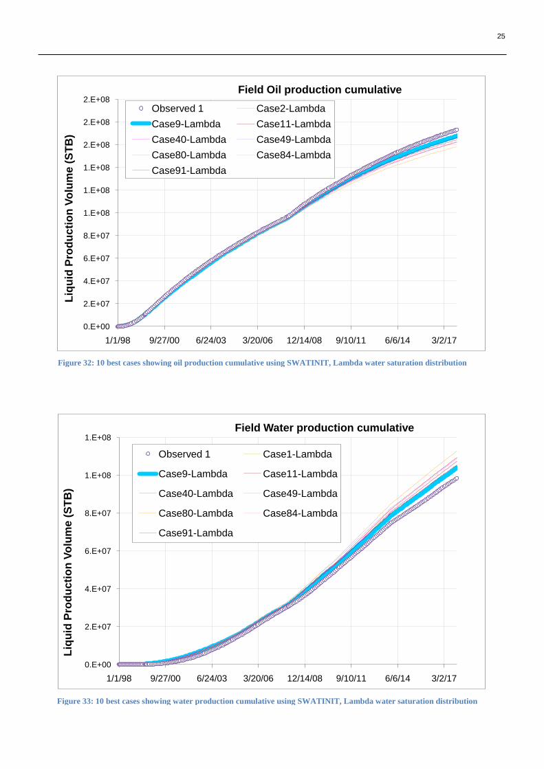
25

0.E+00

2.E+07

4.E+07

6.E+07

8.E+07

1.E+08

1.E+08

1/1/98 9/27/00 6/24/03 3/20/06 12/14/08 9/10/11 6/6/14 3/2/17

Liq

uid

Pro

du

cti

on

Vo

lum

e (

ST

B)






Case91-Lambda

0.E+00

2.E+07

4.E+07

6.E+07

8.E+07

1.E+08

1.E+08

1.E+08

2.E+08

2.E+08

2.E+08

1/1/98 9/27/00 6/24/03 3/20/06 12/14/08 9/10/11 6/6/14 3/2/17

Liq

uid

Pro

du

cti

on

Vo

lum

e (

ST

B)






Case91-Lambda

Figure 33: 10 best cases showing water production cumulative using SWATINIT, Lambda water saturation distribution

Figure 32: 10 best cases showing oil production cumulative using SWATINIT, Lambda water saturation distribution

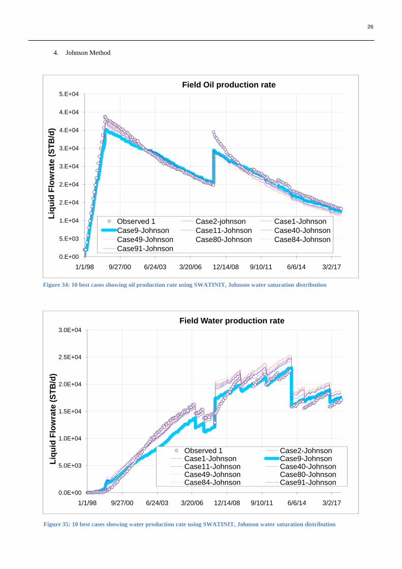
26

0.E+00

5.E+03

1.E+04

2.E+04

2.E+04

3.E+04

3.E+04

4.E+04

4.E+04

5.E+04

1/1/98 9/27/00 6/24/03 3/20/06 12/14/08 9/10/11 6/6/14 3/2/17

Liq

uid

Flo

wra

te (

ST

B/d

)


Observed 1 Case2-johnson Case1-Johnson

Case9-Johnson Case11-Johnson Case40-Johnson

Case49-Johnson Case80-Johnson Case84-Johnson

Case91-Johnson

0.0E+00

5.0E+03

1.0E+04

1.5E+04

2.0E+04

2.5E+04

3.0E+04

1/1/98 9/27/00 6/24/03 3/20/06 12/14/08 9/10/11 6/6/14 3/2/17

Liq

uid

Flo

wra

te (

ST

B/d

)


Observed 1 Case2-JohnsonCase1-Johnson Case9-JohnsonCase11-Johnson Case40-JohnsonCase49-Johnson Case80-JohnsonCase84-Johnson Case91-Johnson

4. Johnson Method

Figure 35: 10 best cases showing water production rate using SWATINIT, Johnson water saturation distribution

Figure 34: 10 best cases showing oil production rate using SWATINIT, Johnson water saturation distribution

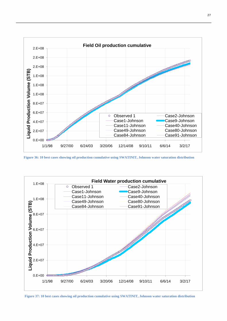
27

0.E+00

2.E+07

4.E+07

6.E+07

8.E+07

1.E+08

1.E+08

1.E+08

2.E+08

2.E+08

2.E+08

1/1/98 9/27/00 6/24/03 3/20/06 12/14/08 9/10/11 6/6/14 3/2/17

Liq

uid

Pro

du

cti

on

Vo

lum

e (

ST

B)



0.E+00

2.E+07

4.E+07

6.E+07

8.E+07

1.E+08

1.E+08

1/1/98 9/27/00 6/24/03 3/20/06 12/14/08 9/10/11 6/6/14 3/2/17

Liq

uid

Pro

du

cti

on

Vo

lum

e (

ST

B)



Figure 37: 10 best cases showing oil production cumulative using SWATINIT, Johnson water saturation distribution

Figure 36: 10 best cases showing oil production cumulative using SWATINIT, Johnson water saturation distribution

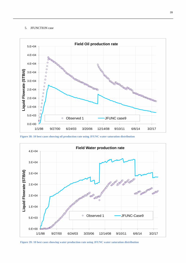
28

0.E+00

5.E+03

1.E+04

2.E+04

2.E+04

3.E+04

3.E+04

4.E+04

4.E+04

5.E+04

1/1/98 9/27/00 6/24/03 3/20/06 12/14/08 9/10/11 6/6/14 3/2/17

Liq

uid

Flo

wra

te (

ST

B/d

)


Observed 1 JFUNC case9

0.E+00

5.E+03

1.E+04

2.E+04

2.E+04

3.E+04

3.E+04

4.E+04

1/1/98 9/27/00 6/24/03 3/20/06 12/14/08 9/10/11 6/6/14 3/2/17

Liq

uid

Flo

wra

te (

ST

B/d

)


Observed 1 JFUNC-Case9

5. JFUNCTION case

Figure 39: 10 best cases showing water production rate using JFUNC water saturation distribution

Figure 38: 10 best cases showing oil production rate using JFUNC water saturation distribution

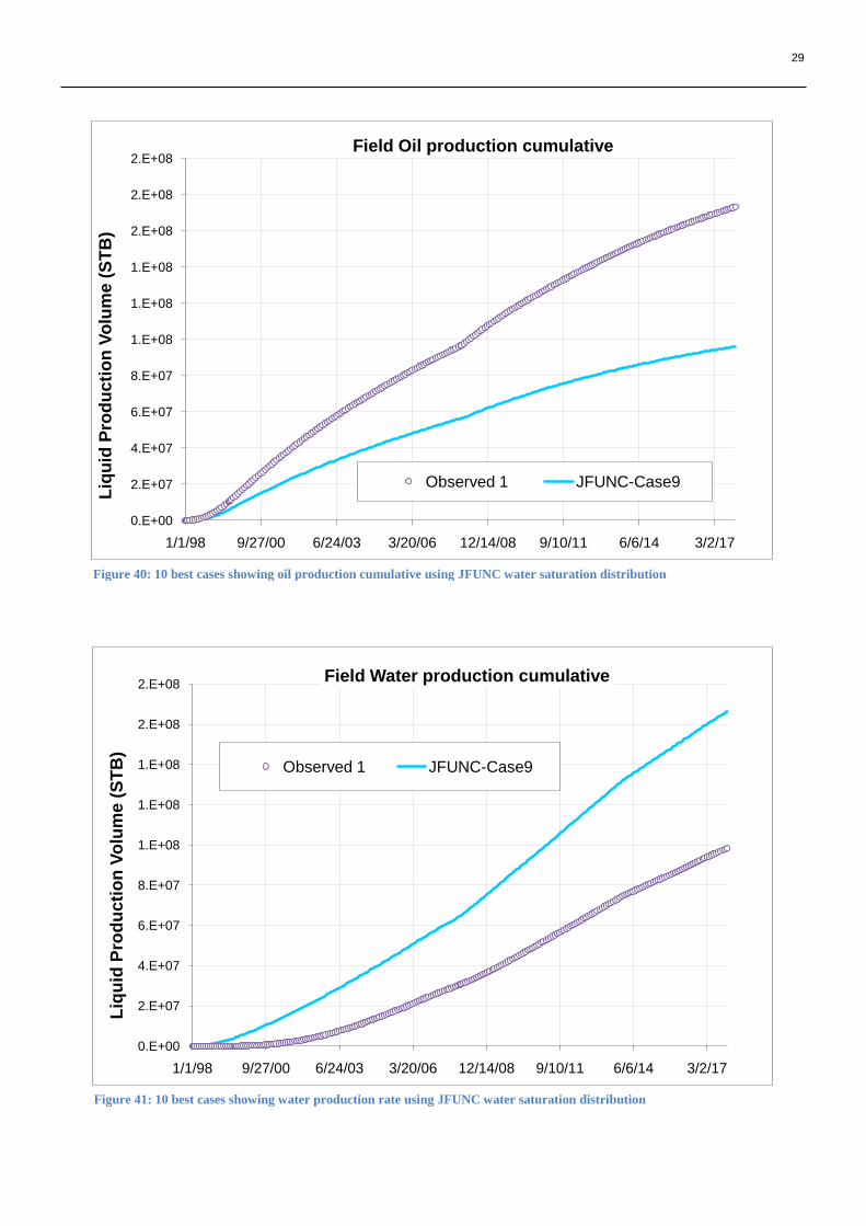
29

0.E+00

2.E+07

4.E+07

6.E+07

8.E+07

1.E+08

1.E+08

1.E+08

2.E+08

2.E+08

2.E+08

1/1/98 9/27/00 6/24/03 3/20/06 12/14/08 9/10/11 6/6/14 3/2/17

Liq

uid

Pro

du

cti

on

Vo

lum

e (

ST

B)



0.E+00

2.E+07

4.E+07

6.E+07

8.E+07

1.E+08

1.E+08

1.E+08

2.E+08

2.E+08

1/1/98 9/27/00 6/24/03 3/20/06 12/14/08 9/10/11 6/6/14 3/2/17

Liq

uid

Pro

du

cti

on

Vo

lum

e (

ST

B)



Figure 40: 10 best cases showing oil production cumulative using JFUNC water saturation distribution

Figure 41: 10 best cases showing water production rate using JFUNC water saturation distribution

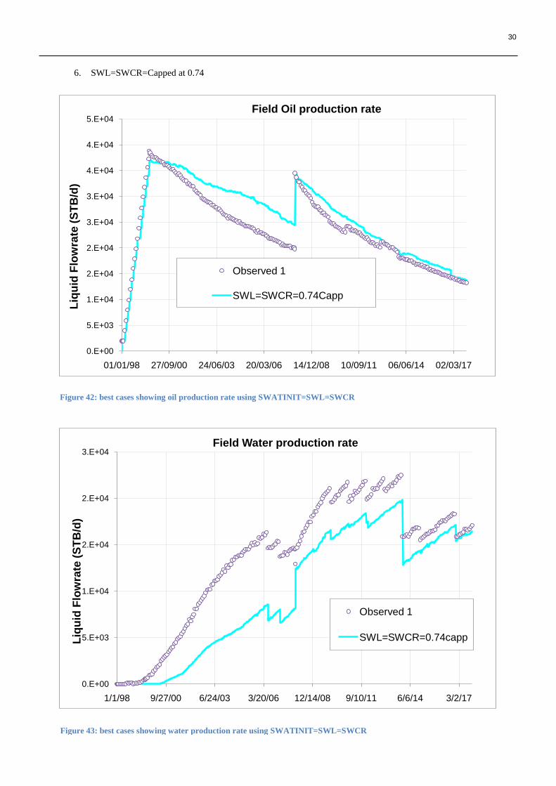
30

0.E+00

5.E+03

1.E+04

2.E+04

2.E+04

3.E+04

3.E+04

4.E+04

4.E+04

5.E+04

01/01/98 27/09/00 24/06/03 20/03/06 14/12/08 10/09/11 06/06/14 02/03/17

Liq

uid

Flo

wra

te (

ST

B/d

)


Observed 1

SWL=SWCR=0.74Capp

0.E+00

5.E+03

1.E+04

2.E+04

2.E+04

3.E+04

1/1/98 9/27/00 6/24/03 3/20/06 12/14/08 9/10/11 6/6/14 3/2/17

Liq

uid

Flo

wra

te (

ST

B/d

)


Observed 1

SWL=SWCR=0.74capp

6. SWL=SWCR=Capped at 0.74

Figure 43: best cases showing water production rate using SWATINIT=SWL=SWCR

Figure 42: best cases showing oil production rate using SWATINIT=SWL=SWCR

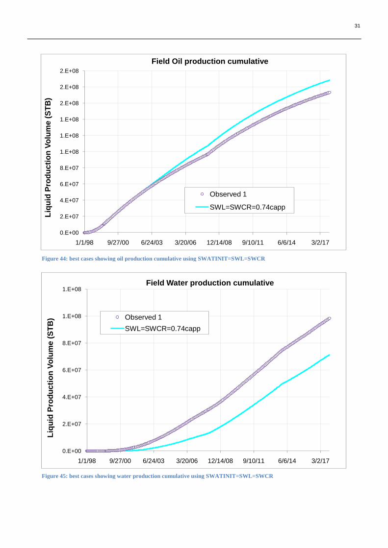
31

0.E+00

2.E+07

4.E+07

6.E+07

8.E+07

1.E+08

1.E+08

1.E+08

2.E+08

2.E+08

2.E+08

1/1/98 9/27/00 6/24/03 3/20/06 12/14/08 9/10/11 6/6/14 3/2/17

Liq

uid

Pro

du

cti

on

Vo

lum

e (

ST

B)


Observed 1

SWL=SWCR=0.74capp

0.E+00

2.E+07

4.E+07

6.E+07

8.E+07

1.E+08

1.E+08

1/1/98 9/27/00 6/24/03 3/20/06 12/14/08 9/10/11 6/6/14 3/2/17

Liq

uid

Pro

du

cti

on

Vo

lum

e (

ST

B)


Observed 1

SWL=SWCR=0.74capp

Figure 45: best cases showing water production cumulative using SWATINIT=SWL=SWCR

Figure 44: best cases showing oil production cumulative using SWATINIT=SWL=SWCR

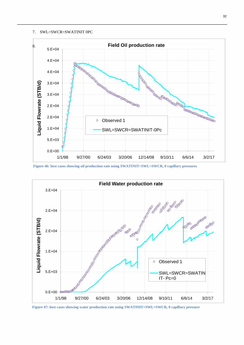
32

0.E+00

5.E+03

1.E+04

2.E+04

2.E+04

3.E+04

3.E+04

4.E+04

4.E+04

5.E+04

1/1/98 9/27/00 6/24/03 3/20/06 12/14/08 9/10/11 6/6/14 3/2/17

Liq

uid

Flo

wra

te (

ST

B/d

)


Observed 1

SWL=SWCR=SWATINIT-0Pc

0.E+00

5.E+03

1.E+04

2.E+04

2.E+04

3.E+04

1/1/98 9/27/00 6/24/03 3/20/06 12/14/08 9/10/11 6/6/14 3/2/17

Liq

uid

Flo

wra

te (

ST

B/d

)


Observed 1

SWL=SWCR=SWATINIT- Pc=0

7. SWL=SWCR=SWATINIT 0PC

8.

Figure 46: best cases showing oil production rate using SWATINIT=SWL=SWCR, 0 capillary pressures

Figure 47: best cases showing water production rate using SWATINIT=SWL=SWCR, 0 capillary pressure

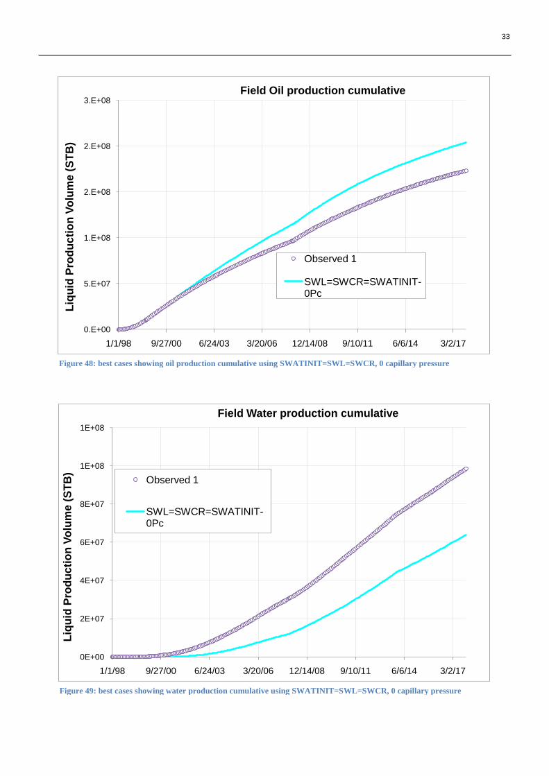
33

0.E+00

5.E+07

1.E+08

2.E+08

2.E+08

3.E+08

1/1/98 9/27/00 6/24/03 3/20/06 12/14/08 9/10/11 6/6/14 3/2/17

Liq

uid

Pro

du

cti

on

Vo

lum

e (

ST

B)


Observed 1


0E+00

2E+07

4E+07

6E+07

8E+07

1E+08

1E+08

1/1/98 9/27/00 6/24/03 3/20/06 12/14/08 9/10/11 6/6/14 3/2/17

Liq

uid

Pro

du

cti

on

Vo

lum

e (

ST

B)


Observed 1


Figure 48: best cases showing oil production cumulative using SWATINIT=SWL=SWCR, 0 capillary pressure

Figure 49: best cases showing water production cumulative using SWATINIT=SWL=SWCR, 0 capillary pressure

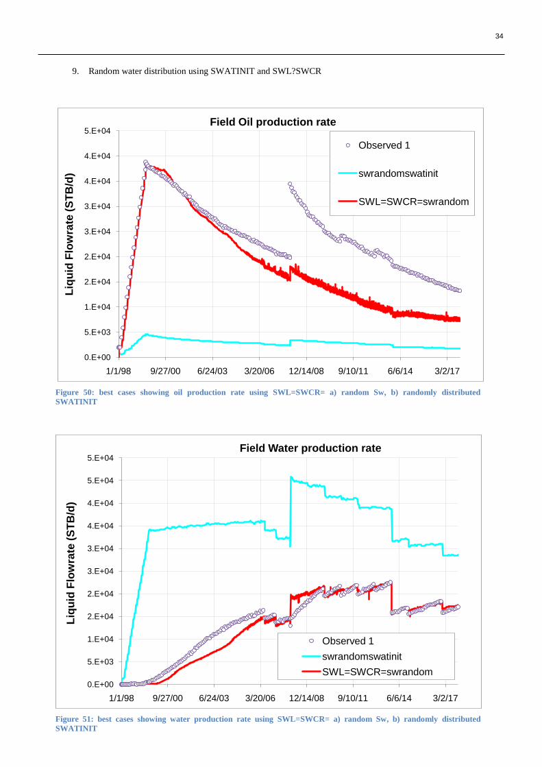
34

0.E+00

5.E+03

1.E+04

2.E+04

2.E+04

3.E+04

3.E+04

4.E+04

4.E+04

5.E+04

1/1/98 9/27/00 6/24/03 3/20/06 12/14/08 9/10/11 6/6/14 3/2/17

Liq

uid

Flo

wra

te (

ST

B/d

)


Observed 1

swrandomswatinit

SWL=SWCR=swrandom

0.E+00

5.E+03

1.E+04

2.E+04

2.E+04

3.E+04

3.E+04

4.E+04

4.E+04

5.E+04

5.E+04

1/1/98 9/27/00 6/24/03 3/20/06 12/14/08 9/10/11 6/6/14 3/2/17

Liq

uid

Flo

wra

te (

ST

B/d

)


Observed 1

swrandomswatinit

SWL=SWCR=swrandom

9. Random water distribution using SWATINIT and SWL?SWCR

Figure 50: best cases showing oil production rate using SWL=SWCR= a) random Sw, b) randomly distributed

SWATINIT

Figure 51: best cases showing water production rate using SWL=SWCR= a) random Sw, b) randomly distributed

SWATINIT

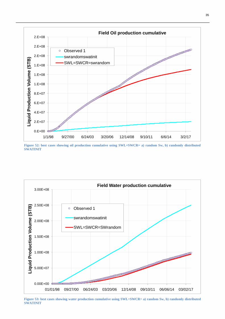
35

0.E+00

2.E+07

4.E+07

6.E+07

8.E+07

1.E+08

1.E+08

1.E+08

2.E+08

2.E+08

2.E+08

1/1/98 9/27/00 6/24/03 3/20/06 12/14/08 9/10/11 6/6/14 3/2/17

Liq

uid

Pro

du

cti

on

Vo

lum

e (

ST

B)


Observed 1

swrandomswatinit

SWL=SWCR=swrandom

0.00E+00

5.00E+07

1.00E+08

1.50E+08

2.00E+08

2.50E+08

3.00E+08

01/01/98 09/27/00 06/24/03 03/20/06 12/14/08 09/10/11 06/06/14 03/02/17

Liq

uid

Pro

du

cti

on

Vo

lum

e (

ST

B)


Observed 1

swrandomswatinit

SWL=SWCR=SWrandom

Figure 53: best cases showing water production cumulative using SWL=SWCR= a) random Sw, b) randomly distributed

SWATINIT

Figure 52: best cases showing oil production cumulative using SWL=SWCR= a) random Sw, b) randomly distributed

SWATINIT

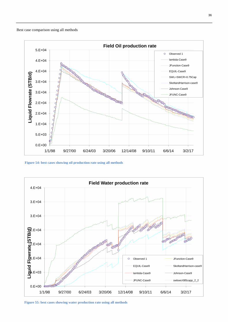
36

0.E+00

5.E+03

1.E+04

2.E+04

2.E+04

3.E+04

3.E+04

4.E+04

4.E+04

5.E+04

1/1/98 9/27/00 6/24/03 3/20/06 12/14/08 9/10/11 6/6/14 3/2/17

Liq

uid

Flo

wra

te (

ST

B/d

)


Observed 1

lambda-Case9

JFunction-Case9

EQUIL-Case9

SWL=SWCR=0.75Cap

SkeltandHarrison-case9

Johnson-Case9

JFUNC-Case9

0.E+00

5.E+03

1.E+04

2.E+04

2.E+04

3.E+04

3.E+04

4.E+04

1/1/98 9/27/00 6/24/03 3/20/06 12/14/08 9/10/11 6/6/14 3/2/17

Liq

uid

Flo

wra

te (

ST

B/d

)


Observed 1 JFunction-Case9

EQUIL-Case9 SkeltandHarrison-case9

lambda-Case9 Johnson-Case9

JFUNC-Case9 swlswcr085capp_2_2

Best case comparison using all methods

Figure 55: best cases showing water production rate using all methods

Figure 54: best cases showing oil production rate using all methods

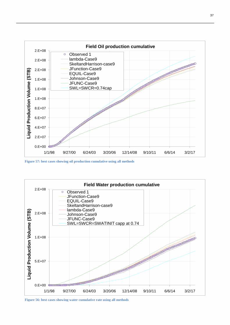
37

0.E+00

2.E+07

4.E+07

6.E+07

8.E+07

1.E+08

1.E+08

1.E+08

2.E+08

2.E+08

2.E+08

1/1/98 9/27/00 6/24/03 3/20/06 12/14/08 9/10/11 6/6/14 3/2/17

Liq

uid

Pro

du

cti

on

Vo

lum

e (

ST

B)


Observed 1lambda-Case9SkeltandHarrison-case9JFunction-Case9EQUIL-Case9Johnson-Case9JFUNC-Case9SWL=SWCR=0.74cap

0.E+00

5.E+07

1.E+08

2.E+08

2.E+08

1/1/98 9/27/00 6/24/03 3/20/06 12/14/08 9/10/11 6/6/14 3/2/17

Liq

uid

Pro

du

cti

on

Vo

lum

e (

ST

B)


Observed 1JFunction-Case9EQUIL-Case9SkeltandHarrison-case9lambda-Case9Johnson-Case9JFUNC-Case9SWL=SWCR=SWATINIT capp at 0.74

Figure 57: best cases showing oil production cumulative using all methods

Figure 56: best cases showing water cumulative rate using all methods

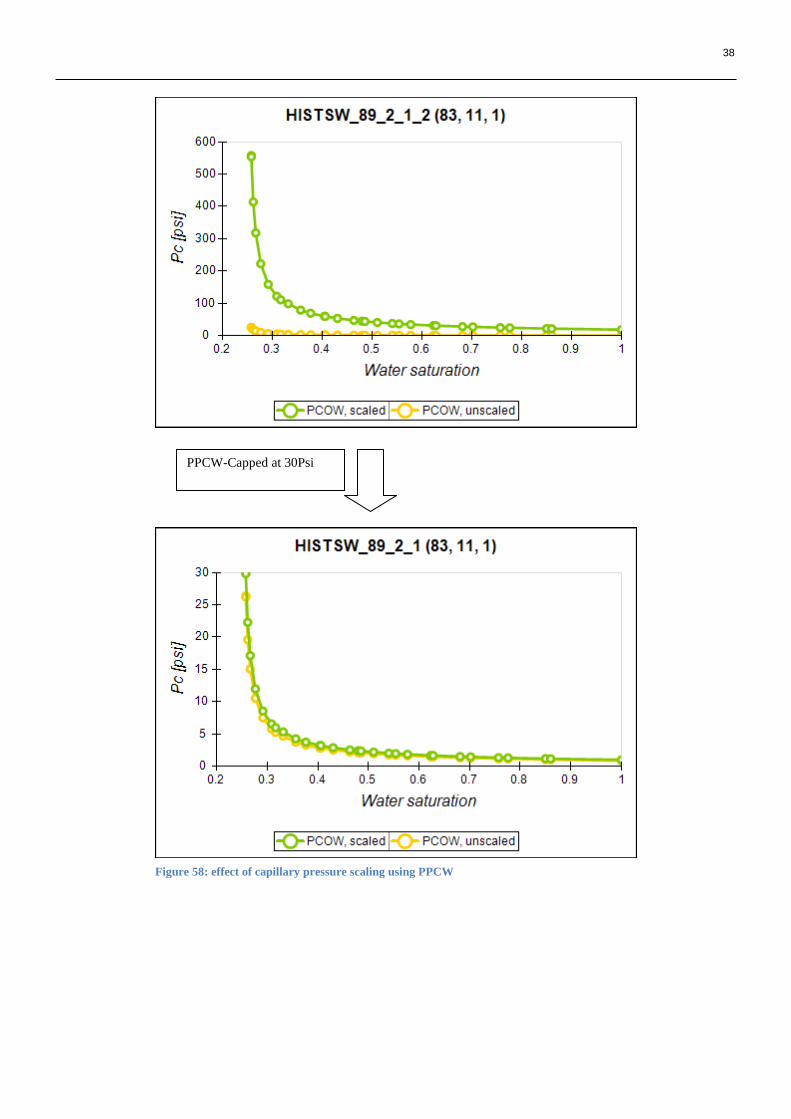
38

PPCW-Capped at 30Psi

Figure 58: effect of capillary pressure scaling using PPCW

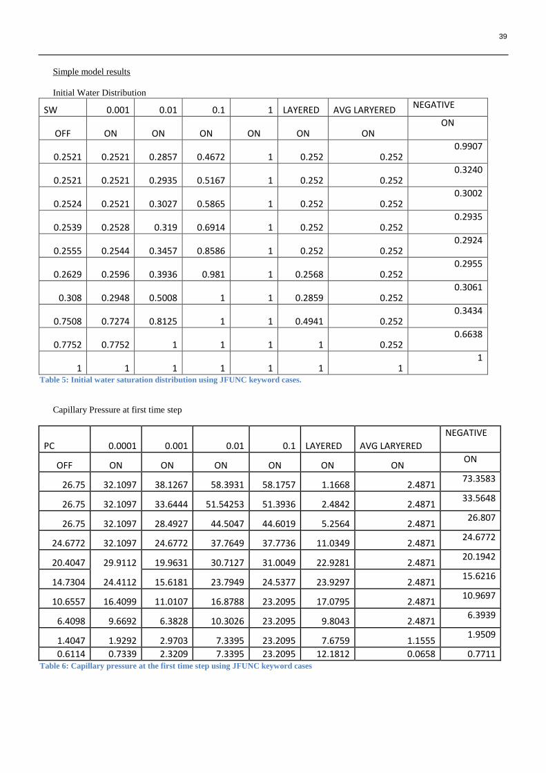
39

Simple model results

Initial Water Distribution

SW 0.001 0.01 0.1 1 LAYERED AVG LARYERED NEGATIVE

OFF ON ON ON ON ON ON ON

0.2521 0.2521 0.2857 0.4672 1 0.252 0.252 0.9907

0.2521 0.2521 0.2935 0.5167 1 0.252 0.252 0.3240

0.2524 0.2521 0.3027 0.5865 1 0.252 0.252 0.3002

0.2539 0.2528 0.319 0.6914 1 0.252 0.252 0.2935

0.2555 0.2544 0.3457 0.8586 1 0.252 0.252 0.2924

0.2629 0.2596 0.3936 0.981 1 0.2568 0.252 0.2955

0.308 0.2948 0.5008 1 1 0.2859 0.252 0.3061

0.7508 0.7274 0.8125 1 1 0.4941 0.252 0.3434

0.7752 0.7752 1 1 1 1 0.252 0.6638

1 1 1 1 1 1 1 1

Table 5: Initial water saturation distribution using JFUNC keyword cases.

Capillary Pressure at first time step

PC 0.0001 0.001 0.01 0.1 LAYERED AVG LARYERED

NEGATIVE

OFF ON ON ON ON ON ON ON

26.75 32.1097 38.1267 58.3931 58.1757 1.1668 2.4871 73.3583

26.75 32.1097 33.6444 51.54253 51.3936 2.4842 2.4871 33.5648

26.75 32.1097 28.4927 44.5047 44.6019 5.2564 2.4871 26.807

24.6772 32.1097 24.6772 37.7649 37.7736 11.0349 2.4871 24.6772

20.4047 29.9112 19.9631 30.7127 31.0049 22.9281 2.4871 20.1942

14.7304 24.4112 15.6181 23.7949 24.5377 23.9297 2.4871 15.6216

10.6557 16.4099 11.0107 16.8788 23.2095 17.0795 2.4871 10.9697

6.4098 9.6692 6.3828 10.3026 23.2095 9.8043 2.4871 6.3939

1.4047 1.9292 2.9703 7.3395 23.2095 7.6759 1.1555 1.9509

0.6114 0.7339 2.3209 7.3395 23.2095 12.1812 0.0658 0.7711 Table 6: Capillary pressure at the first time step using JFUNC keyword cases

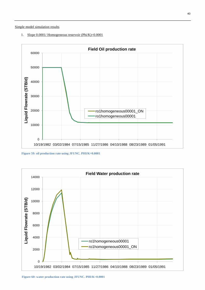
40

0

10000

20000

30000

40000

50000

60000

10/19/1982 03/02/1984 07/15/1985 11/27/1986 04/10/1988 08/23/1989 01/05/1991

Liq

uid

Flo

wra

te (

ST

B/d

)


ro1homogeneous00001_ON

ro1homogeneous00001

0

2000

4000

6000

8000

10000

12000

14000

10/19/1982 03/02/1984 07/15/1985 11/27/1986 04/10/1988 08/23/1989 01/05/1991

Liq

uid

Flo

wra

te (

ST

B/d

)


ro1homogeneous00001


Simple model simulation results

1. Slope 0.0001/ Homogeneous reservoir (Phi/K)=0.0001

Figure 60: water production rate using JFUNC. PHI/K=0.0001

Figure 59: oil production rate using JFUNC. PHI/K=0.0001

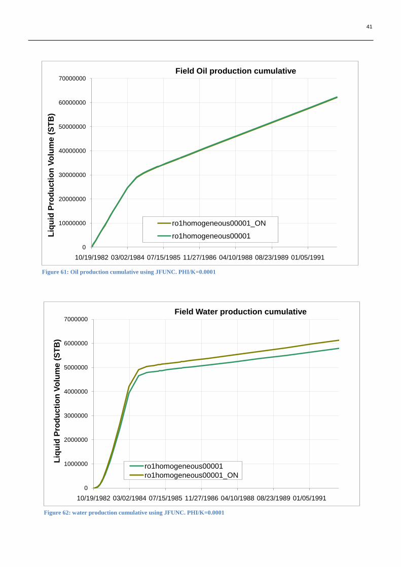
41

0

1000000

2000000

3000000

4000000

5000000

6000000

7000000

10/19/1982 03/02/1984 07/15/1985 11/27/1986 04/10/1988 08/23/1989 01/05/1991

Liq

uid

Pro

du

cti

on

Vo

lum

e (

ST

B)


ro1homogeneous00001


0

10000000

20000000

30000000

40000000

50000000

60000000

70000000

10/19/1982 03/02/1984 07/15/1985 11/27/1986 04/10/1988 08/23/1989 01/05/1991

Liq

uid

Pro

du

cti

on

Vo

lum

e (

ST

B)



ro1homogeneous00001

Figure 61: Oil production cumulative using JFUNC. PHI/K=0.0001

Figure 62: water production cumulative using JFUNC. PHI/K=0.0001

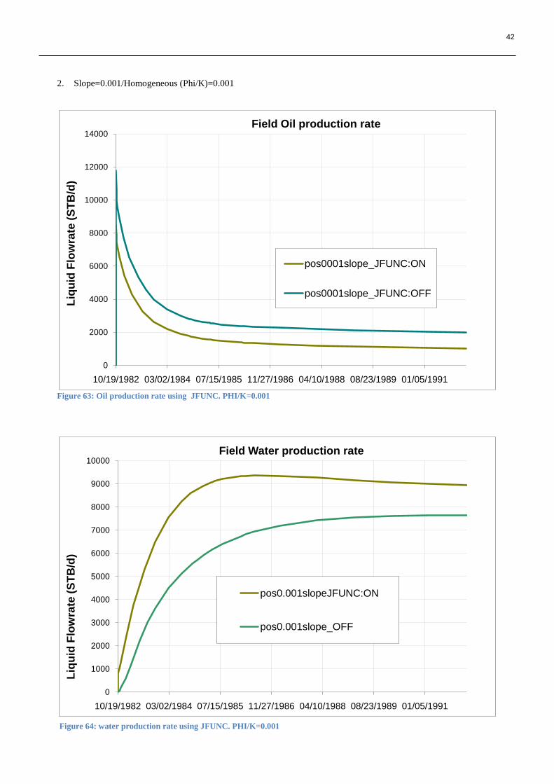
42

0

1000

2000

3000

4000

5000

6000

7000

8000

9000

10000

10/19/1982 03/02/1984 07/15/1985 11/27/1986 04/10/1988 08/23/1989 01/05/1991

Liq

uid

Flo

wra

te (

ST

B/d

)


pos0.001slopeJFUNC:ON

pos0.001slope_OFF

0

2000

4000

6000

8000

10000

12000

14000

10/19/1982 03/02/1984 07/15/1985 11/27/1986 04/10/1988 08/23/1989 01/05/1991

Liq

uid

Flo

wra

te (

ST

B/d

)


pos0001slope_JFUNC:ON

pos0001slope_JFUNC:OFF

2. Slope=0.001/Homogeneous (Phi/K)=0.001

Figure 63: Oil production rate using JFUNC. PHI/K=0.001

Figure 64: water production rate using JFUNC. PHI/K=0.001

43

0

5000000

10000000

15000000

20000000

25000000

30000000

35000000

10/19/1982 03/02/1984 07/15/1985 11/27/1986 04/10/1988 08/23/1989 01/05/1991

Liq

uid

Pro

du

cti

on

Vo

lum

e (

ST

B)


pos0001slope_ON

pos0001slope_OFF

0

1000000

2000000

3000000

4000000

5000000

6000000

7000000

8000000

9000000

10000000

10/19/1982 03/02/1984 07/15/1985 11/27/1986 04/10/1988 08/23/1989 01/05/1991

Liq

uid

Pro

du

cti

on

Vo

lum

e (

ST

B)


pos0001slope_ON

pos0001slope_OFF


Figure 66: Water production cumulative using JFUNC. PHI/K=0.001

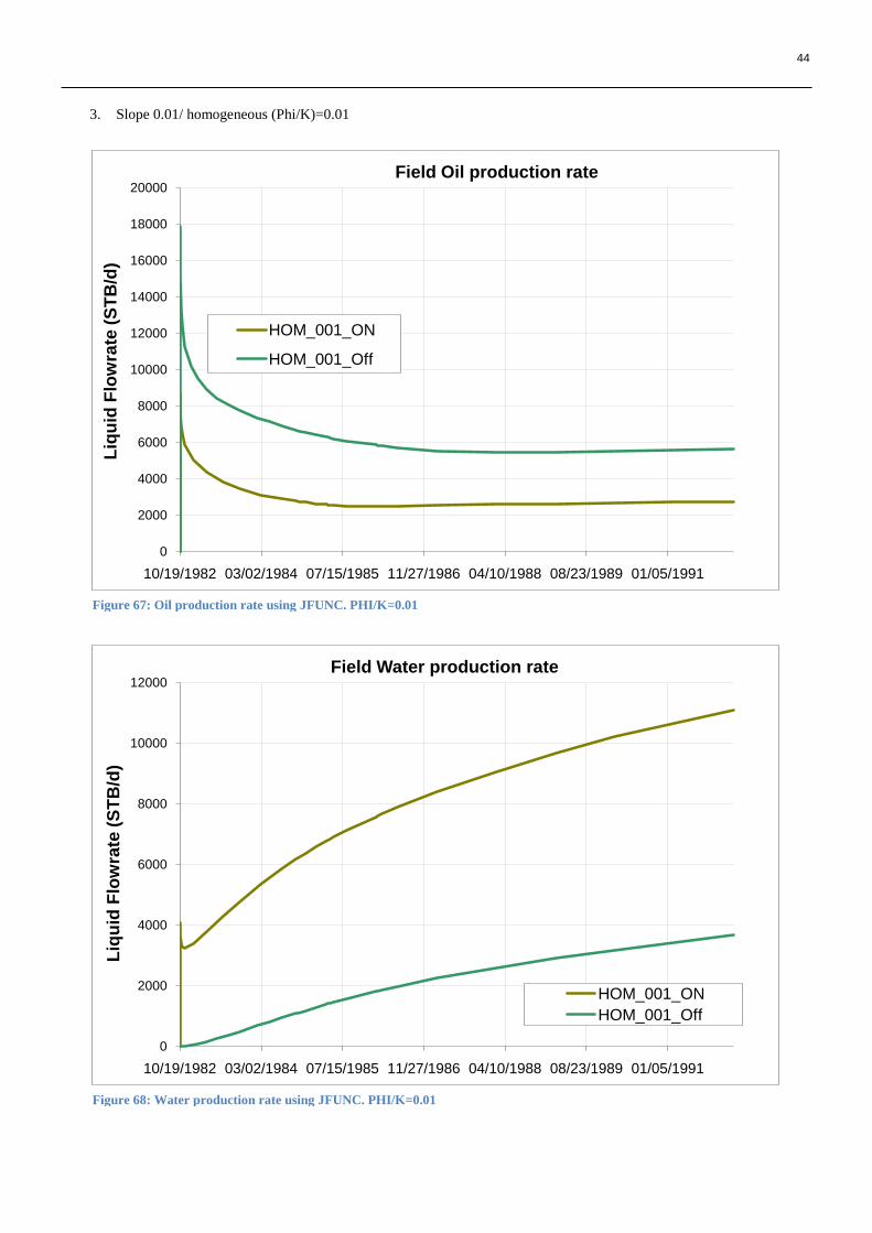
44

0

2000

4000

6000

8000

10000

12000

14000

16000

18000

20000

10/19/1982 03/02/1984 07/15/1985 11/27/1986 04/10/1988 08/23/1989 01/05/1991

Liq

uid

Flo

wra

te (

ST

B/d

)


HOM_001_ON

HOM_001_Off

0

2000

4000

6000

8000

10000

12000

10/19/1982 03/02/1984 07/15/1985 11/27/1986 04/10/1988 08/23/1989 01/05/1991

Liq

uid

Flo

wra

te (

ST

B/d

)


HOM_001_ON

HOM_001_Off

3. Slope 0.01/ homogeneous (Phi/K)=0.01


Figure 68: Water production rate using JFUNC. PHI/K=0.01

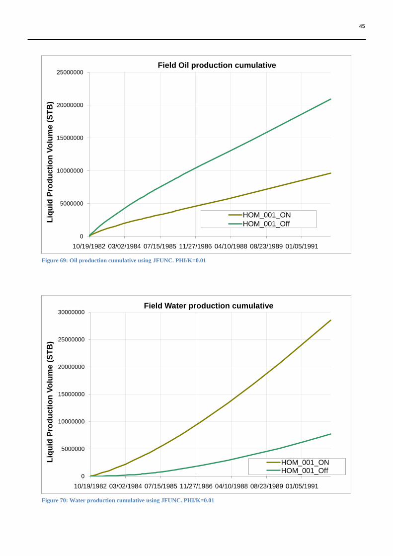
45

0

5000000

10000000

15000000

20000000

25000000

10/19/1982 03/02/1984 07/15/1985 11/27/1986 04/10/1988 08/23/1989 01/05/1991

Liq

uid

Pro

du

cti

on

Vo

lum

e (

ST

B)


HOM_001_ON

HOM_001_Off

0

5000000

10000000

15000000

20000000

25000000

30000000

10/19/1982 03/02/1984 07/15/1985 11/27/1986 04/10/1988 08/23/1989 01/05/1991

Liq

uid

Pro

du

cti

on

Vo

lum

e (

ST

B)


HOM_001_ONHOM_001_Off


Figure 70: Water production cumulative using JFUNC. PHI/K=0.01

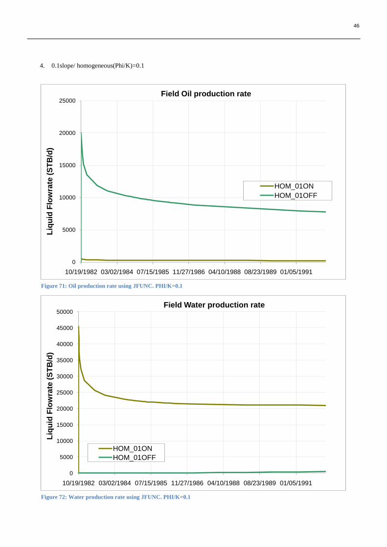
46

0

5000

10000

15000

20000

25000

10/19/1982 03/02/1984 07/15/1985 11/27/1986 04/10/1988 08/23/1989 01/05/1991

Liq

uid

Flo

wra

te (

ST

B/d

)


HOM_01ON

HOM_01OFF

0

5000

10000

15000

20000

25000

30000

35000

40000

45000

50000

10/19/1982 03/02/1984 07/15/1985 11/27/1986 04/10/1988 08/23/1989 01/05/1991

Liq

uid

Flo

wra

te (

ST

B/d

)


HOM_01ON

HOM_01OFF

4. 0.1slope/ homogeneous(Phi/K)=0.1


Figure 72: Water production rate using JFUNC. PHI/K=0.1

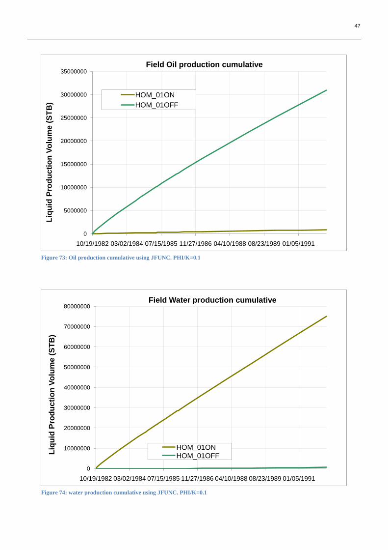
47

0

5000000

10000000

15000000

20000000

25000000

30000000

35000000

10/19/1982 03/02/1984 07/15/1985 11/27/1986 04/10/1988 08/23/1989 01/05/1991

Liq

uid

Pro

du

cti

on

Vo

lum

e (

ST

B)


HOM_01ON

HOM_01OFF

0

10000000

20000000

30000000

40000000

50000000

60000000

70000000

80000000

10/19/1982 03/02/1984 07/15/1985 11/27/1986 04/10/1988 08/23/1989 01/05/1991

Liq

uid

Pro

du

cti

on

Vo

lum

e (

ST

B)


HOM_01ONHOM_01OFF


Figure 74: water production cumulative using JFUNC. PHI/K=0.1

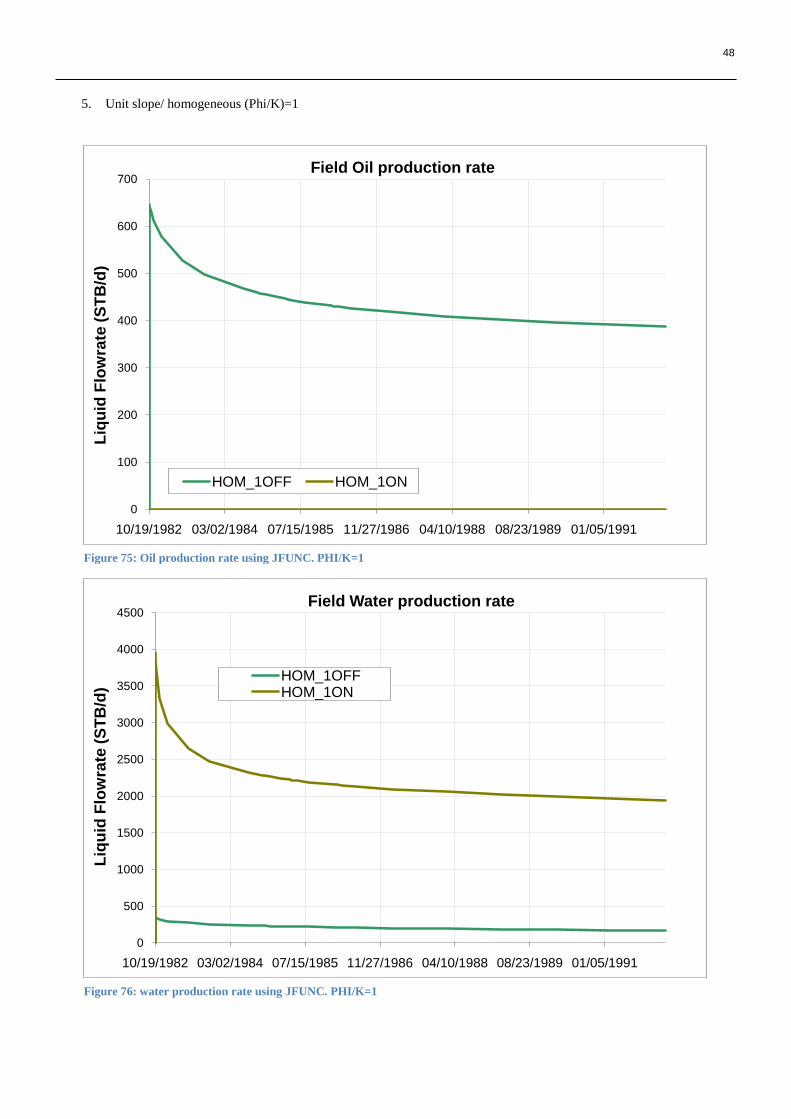
48

0

100

200

300

400

500

600

700

10/19/1982 03/02/1984 07/15/1985 11/27/1986 04/10/1988 08/23/1989 01/05/1991

Liq

uid

Flo

wra

te (

ST

B/d

)


HOM_1OFF HOM_1ON

0

500

1000

1500

2000

2500

3000

3500

4000

4500

10/19/1982 03/02/1984 07/15/1985 11/27/1986 04/10/1988 08/23/1989 01/05/1991

Liq

uid

Flo

wra

te (

ST

B/d

)


HOM_1OFFHOM_1ON

5. Unit slope/ homogeneous (Phi/K)=1

Figure 75: Oil production rate using JFUNC. PHI/K=1

Figure 76: water production rate using JFUNC. PHI/K=1

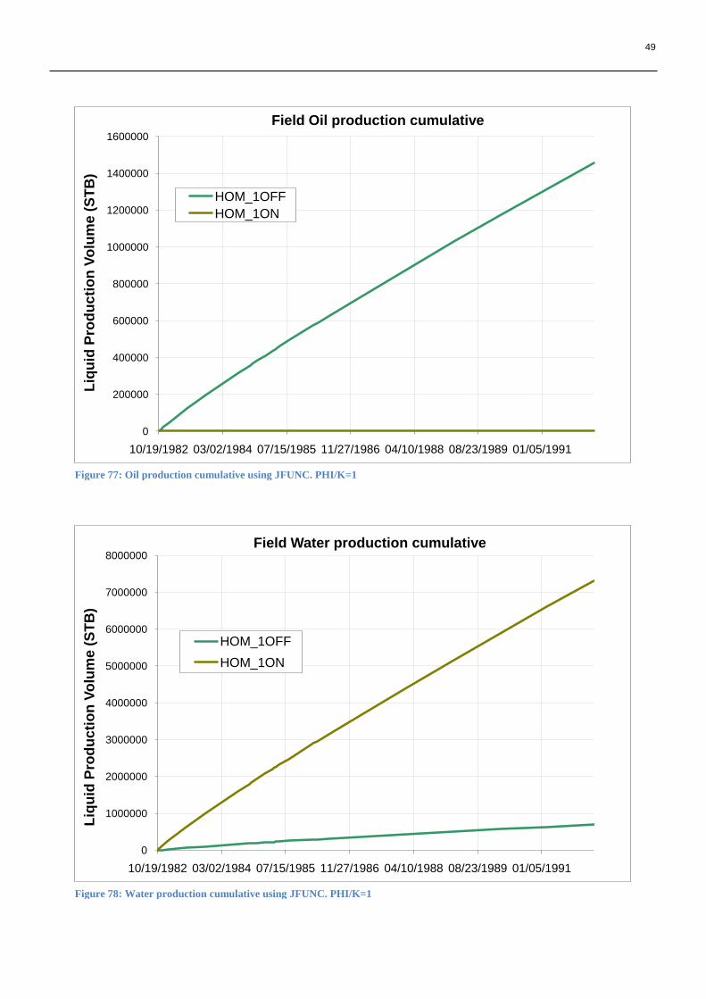
49

0

200000

400000

600000

800000

1000000

1200000

1400000

1600000

10/19/1982 03/02/1984 07/15/1985 11/27/1986 04/10/1988 08/23/1989 01/05/1991

Liq

uid

Pro

du

cti

on

Vo

lum

e (

ST

B)


HOM_1OFF

HOM_1ON

0

1000000

2000000

3000000

4000000

5000000

6000000

7000000

8000000

10/19/1982 03/02/1984 07/15/1985 11/27/1986 04/10/1988 08/23/1989 01/05/1991

Liq

uid

Pro

du

cti

on

Vo

lum

e (

ST

B)


HOM_1OFF

HOM_1ON

Figure 77: Oil production cumulative using JFUNC. PHI/K=1

Figure 78: Water production cumulative using JFUNC. PHI/K=1

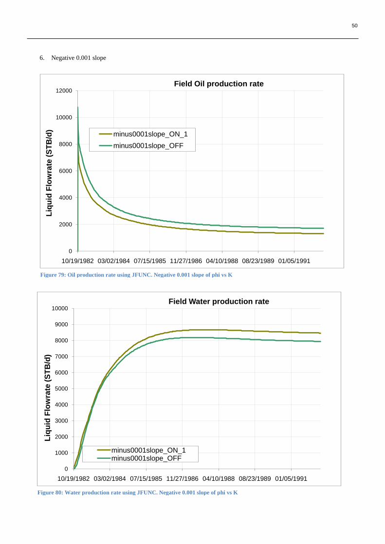
50

0

2000

4000

6000

8000

10000

12000

10/19/1982 03/02/1984 07/15/1985 11/27/1986 04/10/1988 08/23/1989 01/05/1991

Liq

uid

Flo

wra

te (

ST

B/d

)


minus0001slope_ON_1

minus0001slope_OFF

0

1000

2000

3000

4000

5000

6000

7000

8000

9000

10000

10/19/1982 03/02/1984 07/15/1985 11/27/1986 04/10/1988 08/23/1989 01/05/1991

Liq

uid

Flo

wra

te (

ST

B/d

)


minus0001slope_ON_1minus0001slope_OFF

6. Negative 0.001 slope

Figure 79: Oil production rate using JFUNC. Negative 0.001 slope of phi vs K

Figure 80: Water production rate using JFUNC. Negative 0.001 slope of phi vs K

51

0

1000000

2000000

3000000

4000000

5000000

6000000

7000000

8000000

9000000

10/19/1982 03/02/1984 07/15/1985 11/27/1986 04/10/1988 08/23/1989 01/05/1991

Liq

uid

Pro

du

cti

on

Vo

lum

e (

ST

B)


minus0001slope_ON_1

minus0001slope_OFF

0

5000000

10000000

15000000

20000000

25000000

30000000

10/19/1982 03/02/1984 07/15/1985 11/27/1986 04/10/1988 08/23/1989 01/05/1991

Liq

uid

Pro

du

cti

on

Vo

lum

e (

ST

B)


minus0001slope_ON_1

minus0001slope_OFF

Figure 81: Oil production cumulative using JFUNC. Negative 0.001 slope of phi vs K

Figure 82: water production cumulative using JFUNC. Negative 0.001 slope of phi vs K

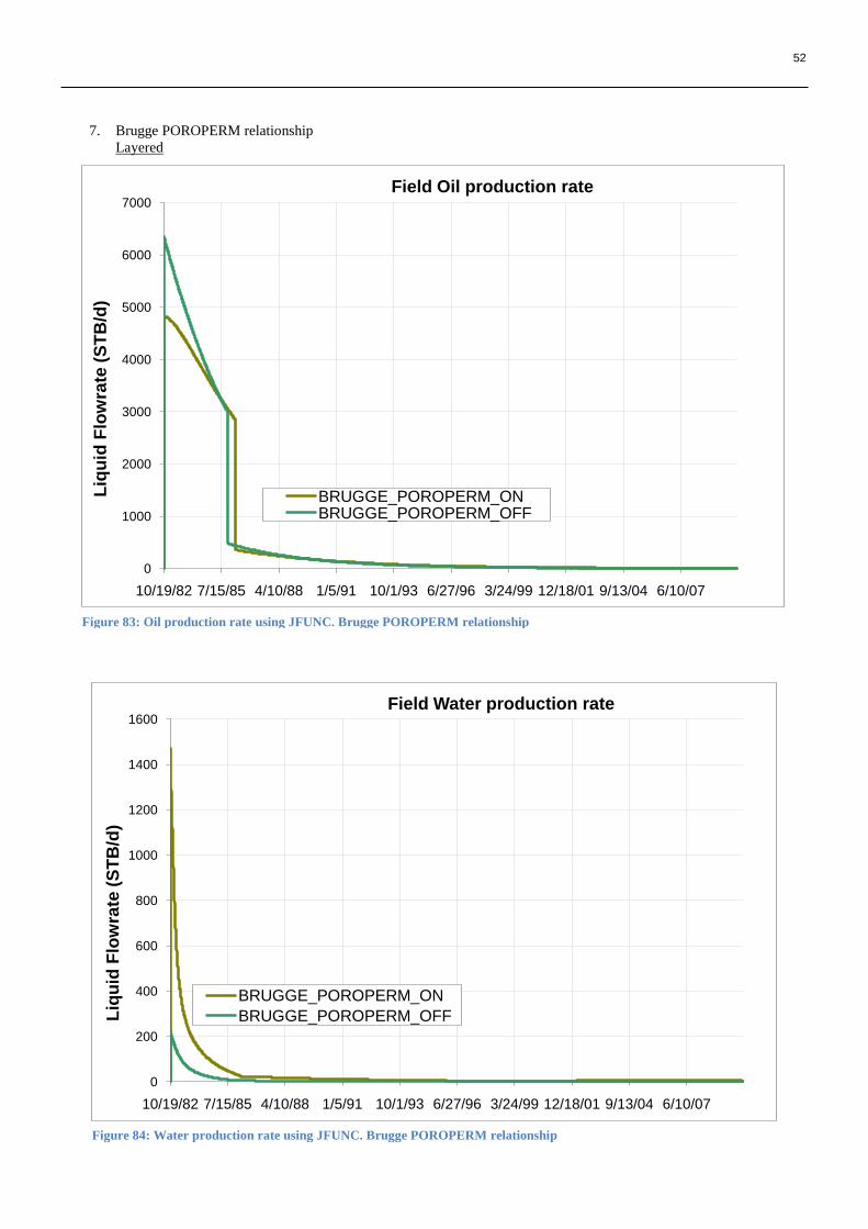
52

0

1000

2000

3000

4000

5000

6000

7000

10/19/82 7/15/85 4/10/88 1/5/91 10/1/93 6/27/96 3/24/99 12/18/01 9/13/04 6/10/07

Liq

uid

Flo

wra

te (

ST

B/d

)


BRUGGE_POROPERM_ONBRUGGE_POROPERM_OFF

0

200

400

600

800

1000

1200

1400

1600

10/19/82 7/15/85 4/10/88 1/5/91 10/1/93 6/27/96 3/24/99 12/18/01 9/13/04 6/10/07

Liq

uid

Flo

wra

te (

ST

B/d

)


BRUGGE_POROPERM_ON

BRUGGE_POROPERM_OFF

7. Brugge POROPERM relationship

Layered

Figure 83: Oil production rate using JFUNC. Brugge POROPERM relationship

Figure 84: Water production rate using JFUNC. Brugge POROPERM relationship

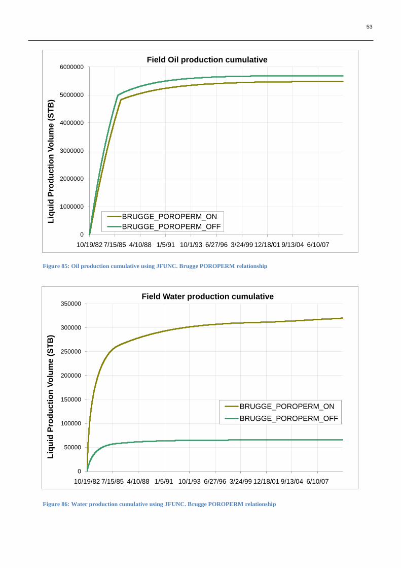
53

0

1000000

2000000

3000000

4000000

5000000

6000000

10/19/82 7/15/85 4/10/88 1/5/91 10/1/93 6/27/96 3/24/99 12/18/01 9/13/04 6/10/07

Liq

uid

Pro

du

cti

on

Vo

lum

e (

ST

B)


BRUGGE_POROPERM_ON

BRUGGE_POROPERM_OFF

0

50000

100000

150000

200000

250000

300000

350000

10/19/82 7/15/85 4/10/88 1/5/91 10/1/93 6/27/96 3/24/99 12/18/01 9/13/04 6/10/07

Liq

uid

Pro

du

cti

on

Vo

lum

e (

ST

B)


BRUGGE_POROPERM_ON

BRUGGE_POROPERM_OFF

Figure 86: Water production cumulative using JFUNC. Brugge POROPERM relationship

Figure 85: Oil production cumulative using JFUNC. Brugge POROPERM relationship

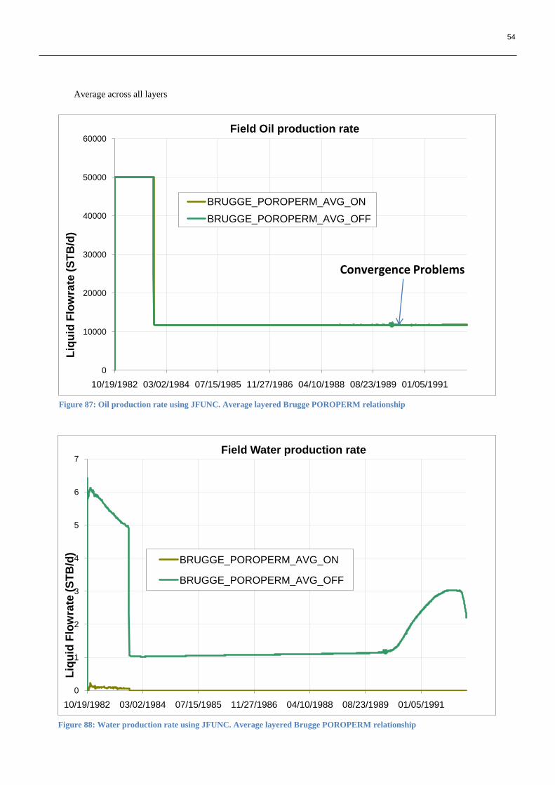
54

0

10000

20000

30000

40000

50000

60000

10/19/1982 03/02/1984 07/15/1985 11/27/1986 04/10/1988 08/23/1989 01/05/1991

Liq

uid

Flo

wra

te (

ST

B/d

)


BRUGGE_POROPERM_AVG_ON

BRUGGE_POROPERM_AVG_OFF

Convergence Problems

0

1

2

3

4

5

6

7

10/19/1982 03/02/1984 07/15/1985 11/27/1986 04/10/1988 08/23/1989 01/05/1991

Liq

uid

Flo

wra

te (

ST

B/d

)




Average across all layers

Figure 87: Oil production rate using JFUNC. Average layered Brugge POROPERM relationship

Figure 88: Water production rate using JFUNC. Average layered Brugge POROPERM relationship

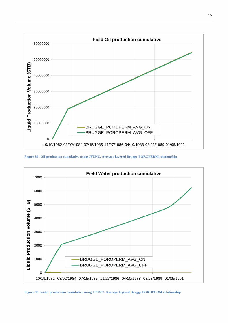
55

0

10000000

20000000

30000000

40000000

50000000

60000000

10/19/1982 03/02/1984 07/15/1985 11/27/1986 04/10/1988 08/23/1989 01/05/1991

Liq

uid

Pro

du

cti

on

Vo

lum

e (

ST

B)




0

1000

2000

3000

4000

5000

6000

7000

10/19/1982 03/02/1984 07/15/1985 11/27/1986 04/10/1988 08/23/1989 01/05/1991

Liq

uid

Pro

du

cti

on

Vo

lum

e (

ST

B)




Figure 90: water production cumulative using JFUNC. Average layered Brugge POROPERM relationship

Figure 89: Oil production cumulative using JFUNC. Average layered Brugge POROPERM relationship

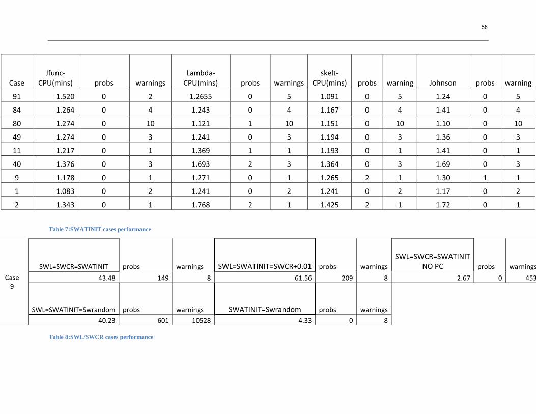
56

Table 7:SWATINIT cases performance

Table 8:SWL/SWCR cases performance

Case Jfunc-

CPU(mins) probs warnings Lambda-

CPU(mins) probs warnings skelt-

CPU(mins) probs warning Johnson probs warning

91 1.520 0 2 1.2655 0 5 1.091 0 5 1.24 0 5

84 1.264 0 4 1.243 0 4 1.167 0 4 1.41 0 4

80 1.274 0 10 1.121 1 10 1.151 0 10 1.10 0 10

49 1.274 0 3 1.241 0 3 1.194 0 3 1.36 0 3

11 1.217 0 1 1.369 1 1 1.193 0 1 1.41 0 1

40 1.376 0 3 1.693 2 3 1.364 0 3 1.69 0 3

9 1.178 0 1 1.271 0 1 1.265 2 1 1.30 1 1

1 1.083 0 2 1.241 0 2 1.241 0 2 1.17 0 2

2 1.343 0 1 1.768 2 1 1.425 2 1 1.72 0 1

Case 9

SWL=SWCR=SWATINIT probs warnings SWL=SWATINIT=SWCR+0.01 probs warnings

SWL=SWCR=SWATINIT NO PC probs warnings

43.48 149 8 61.56 209 8 2.67 0 453

SWL=SWATINIT=Swrandom probs warnings SWATINIT=Swrandom probs warnings 40.23 601 10528 4.33 0 8