Capital Budgeting

MBA FellowsCorporate Finance Learning ModulePart I

Topic Outline

Capital Budgeting Project Classifications Capital Budgeting Decision Criteria Reinvestment Assumptions Post Audit Replacement Chain Approach

Estimating Cash Flows

After-tax cash flows not accounting profits are the basis for evaluating projects.

Incremental Cash Flows - the difference between the cash flows to the firm with the project compared to the cash flows to the firm without adopting the project.

Incremental Cash Flows

Indirect costs such as: increases in cash balances, receivables, and inventory necessitated by the project should included.

Sunk Costs - not included because they have already occurred and are not affected by the current decision.

Opportunity Costs

Used to measure resources used in the project.

Opportunity cost of resources are the cash flows they would generate if not used in the project under consideration.

Initial Cash Outlay

New project costs + installation/shipping

Increases in Net Working Capital Net proceeds from the sale of existing

assets. Taxes associated with the sale of

existing assets or the purchase of a new one.

Incremental After Cash Flows

Increased revenue offset by increased expenses.

Labor and material savings Increases in overhead Tax Savings from an increase in

depreciation expense

Terminal Cash Flows

Cash flows occurring at the end of the of a project’s life must be included in the analysis.

Recovery of new working capital - can be a cash inflow, but has not tax consequences.

Incremental Salvage Value

Incremental Salvage Value

The difference between the salvage value with the project and without the project.

Sale of Asset > Book Value: Gain/Taxes due.

Sale of Asset < Book Value: Loss/Tax savings.

Sale of Asset=Book Value: No taxes

Salvage Value & Taxes

Gain - taxes as operating income, with taxes due equal to the marginal tax rate times the amount of the gain.

Loss - treated as an operating lost to offset operating income. The tax savings is the marginal tax rate times the amount of the loss.

Interest Charges

Not considered in estimating project’s cash flows so that the project’s value can be considered independent of the method of financing.

The cost of capital (required rate of return) used to discount the project’s cash flows includes these costs.

Depreciation - MACRS

Modified Accelerated Cost Recovery System (MACRS).

Depreciable base - not adjusted for salvage value:

= Cost + Installation/shipping Costs

Summary of After-tax Cash Flows

Initial Outlay Incremental Cash Flows Over the

Project’s Life Terminal Cash Flows

Capital Budgeting

The process of planning for the purchase of long-term assets whose cash flows are expected to continue beyond one year.

Capital Expenditures - cash outlays which are expected to generate future cash benefits (cash inflows).

Capital Budgeting Projects Replacement/maintenance of fixed assets. Expansion of existing products or markets. Expansion into new products or markets. Research Development Investments in education and training. Cost reduction projects.

Capital Budgeting Process

Generating Capital Investment Proposals

Estimating cash flows Evaluating alternatives and selecting

projects to be implemented. Reviewing and auditing prior

investment decisions.

Capital Budgeting Decision Rules

Payback Period Discounted Payback Period Net Present Value (NPV) Internal Rate of Return (IRR) Modified Internal Rate of Return

(MIRR) Profitability Index

Payback Period

The expected number of years it takes to recover a project’s costs, or

The expected number of years required for the cumulative net cash flows from a project to equal the initial cash outlay.

PB = Yr before Recovery + Unrecovered Cost Start of Yr.

Cash Flow During Year

Payback for Project L(Long: Most CFs in out years)

10 8060

0 1 2 3

-100

=

CFt

Cumulative -100 -90 -30 50

PaybackL 2 + 30/80 = 2.375 years

0100

2.4

Project S (Short: CFs come quickly)

70 2050

0 1 23

-100CFt

Cumulative-100 -30 20 40

PaybackS 1 + 30/50 = 1.6 years

100

0

1.6

=

Strengths of Payback:

1. Provides an indication of a project’s risk and liquidity.

2. Easy to calculate and understand.

Weaknesses of Payback:

1. Ignores the TVM.

2. Ignores CFs occurring after the payback period.

Discounted Payback Period Expected number of years required to

recover the initial cash outlay from discounted cash flows

Expected cash flows are discounted at the project’s cost of capital.

Advantages: Easy to calculate and understand Considers time value of money Disadvantage: ignores the time value of

money e cash flows occurring after the payback period.

10 8060

0 1 2 3

CFt

Cumulative-100 -90.91 - 41.32 18.79

Discountedpayback 2 + 41.32/60.11 = 2.7 yrs

Discounted Payback: Uses discountedrather than raw CFs.

PVCFt-100

-10010%

9.09 49.59 60.11

=

Recover invest. + cap. costs in 2.7 yrs.

Net Present Value (NPV)

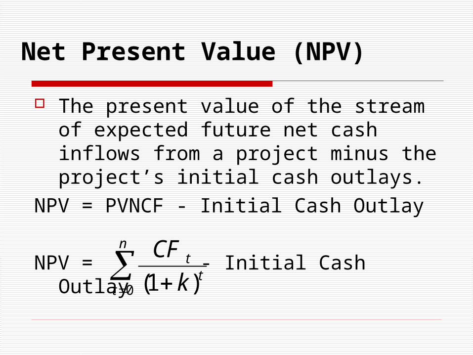
The present value of the stream of expected future net cash inflows from a project minus the project’s initial cash outlays.

NPV = PVNCF - Initial Cash Outlay

NPV = - Initial Cash Outlay

n

tt

t

k

CF

0 )1(

NPV Decision Rule

Accept project when NPV > 0 The present value of the project’s net

cash flows exceeds the project’s initial outlay.

Reject project when NPV < 0 The present value of the net cash

flows is less than the initial outlay

NPV

Advantages: Accounts for the time value of a project’s

cash flows over its entire life. Easy to use and understand - Positive NPV

projects increase the wealth of the firm’s owners, i.e. (maximizing shareholder wealth).

Accept/Reject Decisions are clear.Disadvantages Requires detailed long-term forecasts of the

project’s cash inflows and outflows.

EVA & NPV

NPV is equal to the PV of the project’s future EVAs.

Therefore, accepting positive NPV projects should result in a positive EVA for the company, and a positive MVA.

NPV

CF

kt

nt

t 0 1

.

NPV: Sum of the PVs of inflows and outflows.

Cost often is CF0 and is negative.

.CF

k1

CFNPV 0t

tn

1t

What’s Project L’s NPV?

10 8060

0 1 2 310%

Project L:

-100.00

9.09

49.59

60.1118.79 = NPVL NPVS = $19.98.

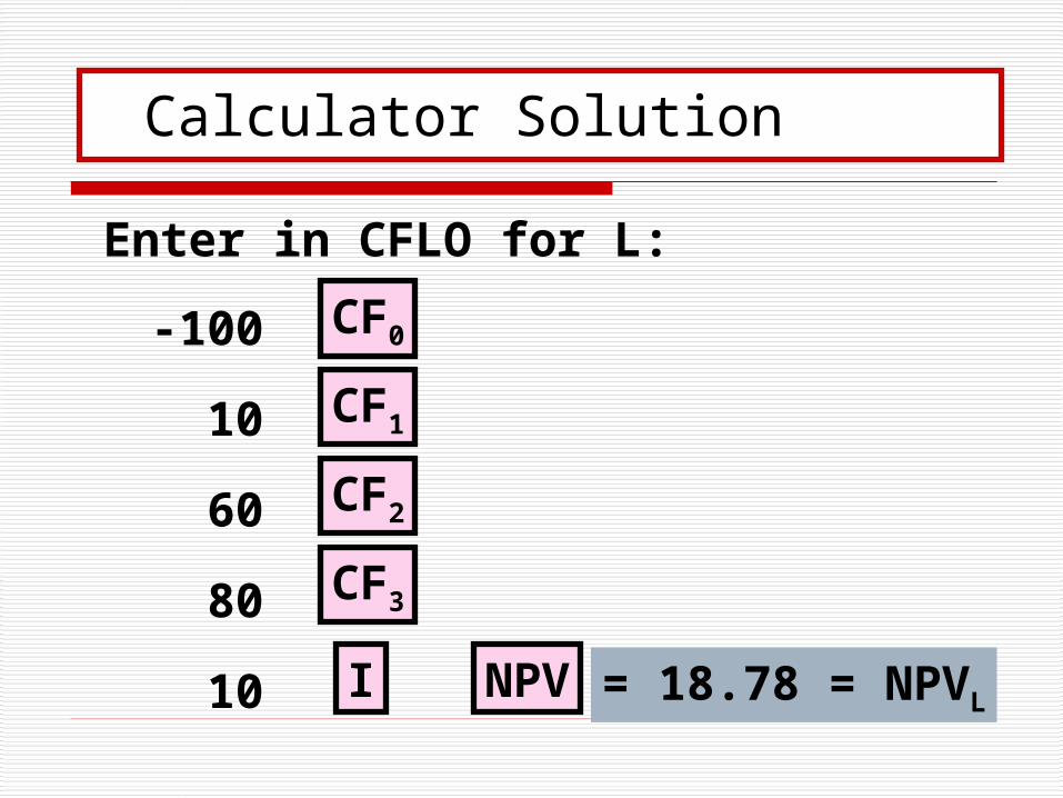
Calculator Solution

Enter in CFLO for L:

-100

10

60

80

10

CF0

CF1

NPV

CF2

CF3

I = 18.78 = NPVL

Rationale for the NPV Method

NPV = PV inflows - Cost= Net gain in wealth.

Accept project if NPV > 0.

Choose between mutually exclusive projects on basis ofhigher NPV. Adds most value.

NPV method: Which project(s) should be accepted?

If Projects S and L are mutually exclusive, accept S because:

NPVs > NPVL . If S & L are independent, accept

both; NPV > 0.

Internal Rate of Return (IRR)

The discount rate which equates the PV of the net cash flows of the project with the PV of the initial investment.

Or, the discount rate which results in a NPV equal to zero.

NPV = 0 =

n

tt

t

IRR

CF

0 )1(

IRR

Disadvantages: Requires detailed long term forecasts

of the incremental benefits and costs. Unusual cash flow patterns (inflows

and outflows) can result in multiple IRRs.

Assumes cash flows over the life of the project are reinvested at the IRR.

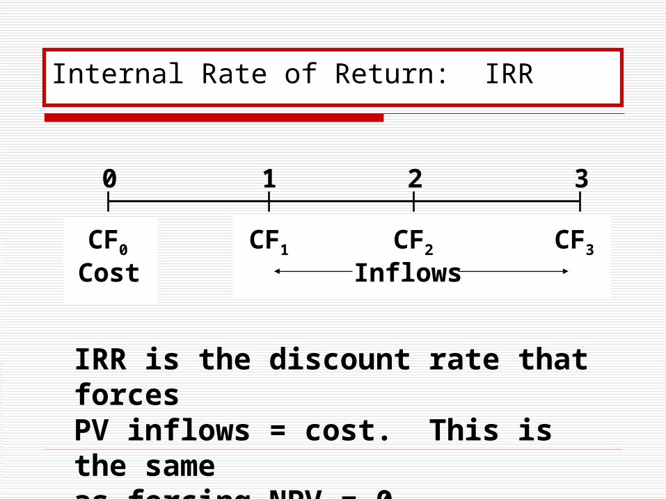
Internal Rate of Return: IRR

0 1 2 3

CF0 CF1 CF2 CF3

Cost Inflows

IRR is the discount rate that forcesPV inflows = cost. This is the sameas forcing NPV = 0.

t

nt

t

CF

kNPV

0 1.

t

nt

t

CF

IRR

0 10.

NPV: Enter k, solve for NPV.

IRR: Enter NPV = 0, solve for IRR.

What’s Project L’s IRR?

10 8060

0 1 2 3IRR = ?

-100.00

PV3

PV2

PV1

0 = NPV

Enter CFs in CFLO, then press IRR:IRRL = 18.13%. IRRS = 23.56%.

40 40 40

0 1 2 3IRR = ?

Find IRR if CFs are constant:

-100

Or, with CFLO, enter CFs and press IRR = 9.70%.

3 -100 40 0

9.70%N I/YR PV PMT FV

INPUTS

OUTPUT

90 1,09090

0 1 2 10IRR = ?

Q. How is a project’s IRRrelated to a bond’s YTM?

A. They are the same thing.A bond’s YTM is the IRRif you invest in the bond.

-1,134.2

IRR = 7.08% (use TVM or CFLO).

...

Rationale for the IRR Method

If IRR > WACC, then the project’s rate of return is greater than its cost-- some return is left over to boost stockholders’ returns.

Example: WACC = 10%, IRR = 15%.Profitable.

Steps in Determining NPV, IRR

1. Estimate CFs (inflows & outflows).

2. Assess riskiness of CFs.

3. Determine k = WACC for project.

4. Find NPV and/or IRR.

5. Accept if NPV > 0 and/or IRR > WACC.

NPV vs. IRR

NPV assumes that the project’s cash flows are reinvested at the the cost of capital.

IRR assumes that the project’s cash flows are reinvested at the IRR.

When 2 or more mutually exclusive projects are acceptable using the IRR and NPV criteria,, and if the two criteria disagree, which is best, the NPV criteria is generally preferred.

Reinvestment Rate Assumptions

NPV assumes reinvest at k (opportunity cost of capital).

IRR assumes reinvest at IRR. Reinvest at opportunity cost, k, is

more realistic, so NPV method is best. NPV should be used to choose between mutually exclusive projects.

NPV and IRR always lead to the same accept/reject decision for independent projects:

k > IRRand NPV < 0.

Reject.

NPV ($)

k (%)IRR

IRR > kand NPV > 0

Accept.

Mutually Exclusive Projects

k 8.7 k

NPV

%

IRRS

IRRL

L

S

k < 8.7: NPVL> NPVS , IRRS > IRRL

CONFLICT

k > 8.7: NPVS> NPVL , IRRS > IRRL

NO CONFLICT

To Find the Crossover Rate

1. Find cash flow differences between the projects. See data at beginning of the case.

2. Enter these differences in CFLO register, then press IRR. Crossover rate = 8.68%, rounded to 8.7%.

3. Can subtract S from L or vice versa, but better to have first CF negative.

4. If profiles don’t cross, one project dominates the other.

Two Reasons NPV Profiles Cross

1. Size (scale) differences. Smaller project frees up funds at t = 0 for investment. The higher the opportunity cost, the more valuable these funds, so high k favors small projects.

2. Timing differences. Project with faster payback provides more CF in early years for reinvestment. If k is high, early CF especially good, NPVS > NPVL.

Modified IRR (MIRR)

Discount rate that equates the present value of the project’s cash outflows with the present value of the project’s terminal value.

Terminal Value - the sum of the future value of the project’s cash inflows compounded at the required rate of return

MIRR

Addresses the reinvestment assumption of IRR and the multiple IRR problem.

Allows the decision maker to to directly specify the appropriate reinvestment rate.

Key Assumption - all cash project inflows are invested at the required rate of return until the termination of the project.

MIRR

Terminal value - take after-tax cash inflows and find their future value at the end of the project’s life, compounding at the required rate of return.

Then calculate the PV of the project’s cash out flows, using the required rate of return.

If the initial outlay is the only cash outflow, then the initial outlay is the PV of the cash outflows.

MIRR the discount rate that equates the PV of the cash outflows with the PV of the project’s terminal value.

MIRR

PV of Costs = PV of Terminal Value

n

tnn

ttn

ttt

MIRR

kCIF

k

COF

1

1

)1(0

0

nn

ttt

MIRR

TV

k

COF

1)1(0

MIRR = 16.5%

10.0 80.060.0

0 1 2 310%

66.0 12.1

158.1

MIRR for Project L (k = 10%)

-100.010%

10%

TV inflows-100.0

PV outflowsMIRRL = 16.5%

$100 = $158.1

(1+MIRRL)3

To find TV with 10B, enter in CFLO:

I = 10

NPV = 118.78 = PV of inflows.

Enter PV = -118.78, N = 3, I = 10, PMT = 0.Press FV = 158.10 = FV of inflows.

Enter FV = 158.10, PV = -100, PMT = 0, N = 3.Press I = 16.50% = MIRR.

CF0 = 0, CF1 = 10, CF2 = 60, CF3 = 80

Why use MIRR versus IRR?

MIRR correctly assumes reinvestment at opportunity cost = WACC. MIRR also avoids the problem of multiple IRRs.

Managers like rate of return comparisons, and MIRR is better for this than IRR.

Decision Rule

MIRR and NPV will always lead to the same decision and will lead to the same ranking if the projects are of similar size and life.

Profitability Index (PI)

Present value of expected future cash inflows (benefits) to the present value of cash outflows (costs).

PI = PV Benefits/PV of Costs

PI =

n

ttt

n

t tt

k

COFk

CIF

0

0

1

1

Decision Rule

Accept if PI > 1 Reject if PI < 1 Same disadvantages/advantages as

NPV PI is a relative measure (increase in

wealth per dollar of investment) NPV - absolute measure of the wealth

increase.

Post Audit

Comparing actual results with those predicted and determining why differences occurred.

The objective is to improve forecasts and operations and to identify termination opportunities.

Replacement Chain Approach

Used to compare projects with unequal lives.

Calculate the NPV of the project with the longer life and then calculate the NPV of the project with the shorter life over the same period (assuming that this project is repeated).

S and L are mutually exclusive and will be repeated. k = 10%. Which is

better? (000s)

0 1 2 3 4

Project S:(100)

Project L:(100)

60

33.5

60

33.5 33.5 33.5

Replacement Chain

Note that Project S could be repeated after 2 years to generate additional profits.

Can use either replacement chain or equivalent annual annuity analysis to make decision.

S LCF0 -100,000 -100,000CF1 60,000 33,500Nj 2 4I 10 10

NPV 4,132 6,190

NPVL > NPVS. But is L better? Need to perform common life analysis.

Project S with Replication:

NPV = $7,547.

Replacement Chain Approach (000s)

0 1 2 3 4

Project S:(100) (100)

60 60

60(100) (40)

6060

6060

Replacement Chain Approach

Used to compare projects with unequal lives.

Calculate the NPV of the project with the longer life and then calculate the NPV of the project with the shorter life over the same period (assuming that this project is repeated).

S and L are mutually exclusive and will be repeated. k = 10%. Which is

better? (000s)

0 1 2 3 4

Project S:(100)

Project L:(100)

60

33.5

60

33.5 33.5 33.5

Replacement Chain

Note that Project S could be repeated after 2 years to generate additional profits.

Can use either replacement chain or equivalent annual annuity analysis to make decision.

S LCF0 -100,000 -100,000CF1 60,000 33,500Nj 2 4I 10 10

NPV 4,132 6,190

NPVL > NPVS. But is L better? Need to perform common life analysis.

Project S with Replication:

NPV = $7,547.

Replacement Chain Approach (000s)

0 1 2 3 4

Project S:(100) (100)

60 60

60(100) (40)

6060

6060

Compare to Project L NPV = $6,190.Compare to Project L NPV = $6,190.

Or, use NPVs:

0 1 2 3 4

4,1323,4157,547

4,13210%

Replacement Chain Approach (000s)

.

If the cost to repeat S in two years rises to $105,000, which is best? (000s)

NPVS = $3,415 < NPVL = $6,190.Now choose L.NPVS = $3,415 < NPVL = $6,190.Now choose L.

0 1 2 3 4

Project S:(100)

60 60(105) (45)

60 60

EVA & NPV

NPV is equal to the PV of the project’s future EVAs.

Therefore, accepting positive NPV projects should result in a positive EVA for the company, and a positive MVA (market value added).