WP/15/80

Capital Control Measures: A New Dataset

Andrés Fernández, Michael W. Klein, Alessandro Rebucci, Martin Schindler, and Martín Uribe

2

© 2015 International Monetary Fund WP/15/80

IMF Working Paper

Institute for Capacity Development

Capital Control Measures: A New Dataset1

Prepared by Andrés Fernández, Michael W. Klein, Alessandro Rebucci, Martin Schindler, and Martín Uribe

Authorized for distribution by Norbert Funke

April 2015

Abstract

This paper presents a new dataset of capital control restrictions on both inflows and outflows of 10 categories of assets for 100 countries over the period 1995 to 2013. Building on the data in Schindler (2009) and other datasets based on the analysis of the IMF’s Annual Report on Exchange Arrangements and Exchange Restrictions (AREAER), this dataset includes additional asset categories, more countries, and a longer time period. The paper discusses in detail the construction of the dataset and characterizes the data with respect to the prevalence and correlation of controls across asset categories and between controls on inflows and controls on outflows, the aggregation of the separate categories into broader indicators, and the comparison of this dataset with other indicators of capital controls.

JEL Classification Numbers: F3, F36, F38 Keywords: capital control measures, capital flows; international financial integration Author’s E-Mail Address: andresf@iadb.org, michael.klein@tufts.edu, arebucci@jhu.edu, mschindler@imf.org, martin.uribe@columbia.edu

1 Author affiliations: Fernández: InterAmerican Development Bank; Klein: Fletcher School, Tufts University & NBER; Rebucci: Carey Business School, Johns Hopkins University; Schindler: International Monetary Fund & Joint Vienna Institute; Uribe: Columbia University & NBER. We thank Javier Caicedo for excellent research assistance. The information and opinions presented in this work are entirely those of the authors, and express or imply no endorsement by the Inter-American Development Bank, the International Monetary Fund, the Board of Executive Directors of either institution, or the countries they represent. The dataset is available for download at http://www.nber.org/data/international-finance/.

This Working Paper should not be reported as representing the views of the IMF. The views expressed in this Working Paper are those of the author(s) and do not necessarily represent those of the IMF or IMF policy. Working Papers describe research in progress by the author(s) and are published to elicit comments and to further debate.

3

CONTENTS PAGE

Abstract ......................................................................................................................................2 

I. Introduction ............................................................................................................................4 

II. Constructing the Capital Control Indicators..........................................................................7 

III. Characteristics of the Capital Control Indicators ...............................................................13 

IV. Aggregate Indicators ..........................................................................................................20 

V. Conclusions .........................................................................................................................28 

VI. References ..........................................................................................................................30  TABLES Table 1: Asset and Transaction Categories for Capital Control Measures ..............................10 Table 2: Countries In Data Set, By Income Groups, With Open/Gate/Wall Category ...........14 Table 3: Prevalence of Controls, 100 Countries, 1995 – 2013, by Asset Sub-Categories.......16 Table 4: Cross-Category Correlations, All 100 Countries, 1995-2013, ..................................17 Table 5A: Cross-Category Correlations, 47 Gate Countries, 1995-2013 ................................19 Table 5B: Cross-Category Correlations, 53 Open and Wall Countries, 1995-2013 ................19 Table 6: Correlation between Nine-Asset Aggregate Capital Controls and Excluded Asset Category ...................................................................................................................................25 Table 7: Correlations among Aggregate Capital Controls Measures ......................................26  FIGURES Figure 1: Proportion of Observations with Controls................................................................15 Figure 2A: Average Controls on Inflows by Income Groups ..................................................21 Figure 2B: Average Controls on Outflows by Income Groups ...............................................22 Figure 3: Inflow Controls vs. Outflow Controls ......................................................................23 Figure 4: Comparison of Aggregate Indicators .......................................................................28  REFERENCES References ................................................................................................................................30 

4

I. INTRODUCTION

International capital flows are central to international macroeconomics. The interaction between

the monetary and exchange rate policies of a country depends upon its stance towards capital

mobility, as described by the policy trilemma. The ability of a government and its citizens to

borrow and lend abroad allows domestic investment to diverge from domestic savings, which

can promote economic efficiency and growth. In addition, international portfolio diversification

is a potentially important means by which individuals can smooth consumption and undertake

risky investments that would otherwise be unattractive. On a less salutary note, international

capital flows are also blamed for being an important vector through which economic

disturbances are spread across countries, or as a means by which investors prompt a sudden stop

that causes an economy to crash.

This range of potential outcomes from the international trade in assets has contributed to

varying attitudes towards capital flows, as well as towards capital controls. Controversies over

international capital flows have a long history. For example, in 1920 J.M. Keynes wrote

elegiacally of a pre-war time when a person could “…adventure his wealth in the natural

resources and new enterprises of any quarter of the world...” (The Economic Consequences of the

Peace, Chapter II). But he took a very different tone in a 1933 speech in Dublin when he stated

“… let goods be home-spun whenever it is reasonable and conveniently possible and, above all,

let finance be national.”2

Keynes’ negative view of international capital flows in the midst of the Great Depression

echoes through time in more contemporary calls for capital controls, especially in the wake of

the recent current economic and financial crisis. While capital controls were pervasive during the

Bretton Woods era, they were reduced or eliminated beginning in the late 1970s, and,

increasingly, in the 1980s and 1990s. The title of Rudiger Dornbusch’s 1998 article “Capital

Controls: An Idea Whose Time is Gone” reflects a broad consensus at that time. But attitudes

began to shift in response to the economic crises in the late 1990s (Rodrik, 1998; Bhagwati,

1998). These changes were far from a fringe view; in 2002, Kenneth Rogoff, then serving as the

Chief Economist and Director of Research of the International Monetary Fund wrote in the

2 Quoted in Skidelsky (1992: 477).

5

Fund’s publication Finance and Development “These days everyone agrees that a more eclectic

approach to capital account liberalization is required.”

The Great Recession has spurred a further reevaluation of the appropriate role of capital

controls. Countries as diverse as Brazil and Switzerland considered (and in the case of Brazil,

implemented) controls on inflows in the face of currency appreciation, while Iceland introduced

controls on outflows at the time of its crisis. A number of recent IMF staff studies and policy

papers accept the use of capital controls as part of a country’s “policy toolkit” under certain

circumstances, a shift that The Economist magazine dubbed “The Reformation.”3 Even stronger

calls for a greater role for capital controls include Jeanne, Subramanian and Williamson (2012)

and Rey (2013). Some of these policy prescriptions are consistent with a new branch of

theoretical research in which capital controls contribute to financial stability and macroeconomic

management.4 The empirical research of others, however, emphasizes the ineffectiveness and

potential costs of capital controls.5

The evolving nature of the debate on capital controls, and the policy prescriptions that

follow, suggest that further careful empirical analysis is needed. One challenge facing empirical

researchers in this area concerns the availability of indicators of capital controls. Although some

empirical research addresses this challenge by considering the experience of a specific country,6

broader, cross-country analyses require panel data reflecting the experience of a range of

countries. While a number of panel data sets exist, those with broad time and/or country

coverage are typically hampered by a lack of granularity (for example, Chinn and Ito, 2006, and

Quinn, 1997), often providing little information beyond a broad index of “capital account

3 Examples of IMF studies include Ostry et al. (2010) and Ostry et al. (2011). The article in The Economist appeared in the April 7, 2011 issue.

4 For just a few examples, see Korinek (2010), Bianchi (2011), Farhi and Werning (2012), Jeanne (2012), Schmitt-Grohé and Uribe (2012), and Benigno et al. (2014).

5 See, for example, Forbes (2007), Binici, Hutchison and Schindler (2010), Klein (2012), Prati, Schindler and Valenzuela (2012), and Klein and Shambaugh (2015).

6 See, for example, studies of the experiences of Chile by DeGregorio, Edwards and Valdés (2000) and Forbes (2007), and of Brazil by Forbes et al. (2012).

6

openness,” while others with finer granularity have been more limited in terms of sample

coverage (such as Schindler, 2009, Miniane, 2004, and Tamirisa, 1999).7

In this paper, we introduce a new dataset based on the methodology in Schindler (2009),

but including more countries, more asset categories and more years. In particular, the new

dataset reports the presence or absence of capital controls, on an annual basis, for 100 countries

over the period 1995 to 2013. As discussed in greater detail below, this dataset revises, extends,

and widens the data set originally developed by Schindler (2009), and later expanded by Klein

(2012) and Fernández, Rebucci and Uribe (2014). This dataset’s wide range of countries and its

coverage of a period of changing policies make it a potentially important resource for research

and policy.8

In particular, a distinguishing and important feature of these data is that the information

on capital controls is disaggregated both by whether the controls are on inflows or outflows, and

by 10 different categories of assets. This allows for a more detailed analysis of capital controls,

including an examination of the co-movements of controls on different types of assets, and on

the co-movements of controls on inflows and outflows, as well as the construction of aggregate

measures of controls that are well targeted to the specific nature of the topic being studied.

Variations of such aggregate measures across time serve as one indicator of the intensity of the

application of restrictions on international capital movements.

The next section of the paper discusses the methods used to develop this dataset from

annual information published by the IMF. In Section 3 we discuss some statistics of our

disaggregated dataset, including the correlation across categories of assets and directions of

transactions (that is, controls on inflows or on outflows). Section 4 discusses issues related to

aggregating the asset categories and also compares an aggregated index of our data with two

aggregate indicators that are commonly used in panel estimation, those first introduced in Quinn

(1997) and in Chinn and Ito (2006). We offer some concluding comments in Section 5.

7 See Quinn, Schindler, and Toyoda (2011) for a comprehensive review of existing de jure measures.

8 The dataset is publicly available for download at the National Bureau of Economic Research website (http://www.nber.org/data/international-finance/) or at request from the authors.

7

II. CONSTRUCTING THE CAPITAL CONTROL INDICATORS

Cross-country time series of capital controls typically draw from the IMF’s Annual Report on

Exchange Arrangements and Exchange Restrictions (AREAER).9 The capital control measures

presented in this paper are also based on the de jure information from this source.10 There was a

fundamental change in the reporting on capital controls beginning with the 1996 volume of the

AREAER (providing information for conditions in 1995) when it began including more detailed

information both across a disaggregated set of assets and by distinguishing between controls on

outflows and controls on inflows; thus our data series begin in 1995 and currently include data

through 2013.11 In this section we describe the dataset we have constructed and discuss the

methods we have taken to translate the narrative in the annual volumes into a panel dataset.

The present work revises, extends, and widens the data set originally developed by

Schindler (2009), and later expanded by Klein (2012) and Fernández, Rebucci and Uribe (2014).

Schindler’s dataset covers 91 countries over the period 1995 to 2005, and considers restrictions

on inflows and outflows over six asset categories, namely, equity, bonds, money market,

collective investment, financial credit, and foreign direct investment. Klein (2012) extends

Schindler’s dataset to include the period 2006 to 2010 but limits the coverage to 44 countries and

restrictions on inflows. Fernandez, Rebucci and Uribe (2014) further extend the dataset to the

year 2011 for the original 91 countries in Schindler (2009). They also consider restrictions on

capital inflows and outflows.

The dataset discussed in this paper extends currently available data in three dimensions;

asset categories, countries, and sample period. The four new asset categories are derivatives,

commercial credit, financial guarantees, and real estate. Derivatives are of particular interest,

9 The early works that use the AREAER to create panel data sets of capital controls include Grilli and Milesi-Ferretti (1995), Quinn (1997) and Chinn and Ito (2006).

10 That is, the measures capture legal restrictions, but not whether or to what extent they are enforced. One difficulty in trying to construct empirically-based de facto indicators of capital account restrictions is that there is not a clear benchmark of the gross capital flows consistent with free capital mobility. Furthermore, de facto indicators based on the equalization of rates of return would assume efficient markets, and require making assumptions about investors’ expectations and preferences as well as the correlations of asset returns with other measures of risk.

11 There is very limited coverage for the years 1995 and 1996 for one category of assets, controls on bonds with maturity of greater than one year, and so the data series for this asset begins in 1997.

8

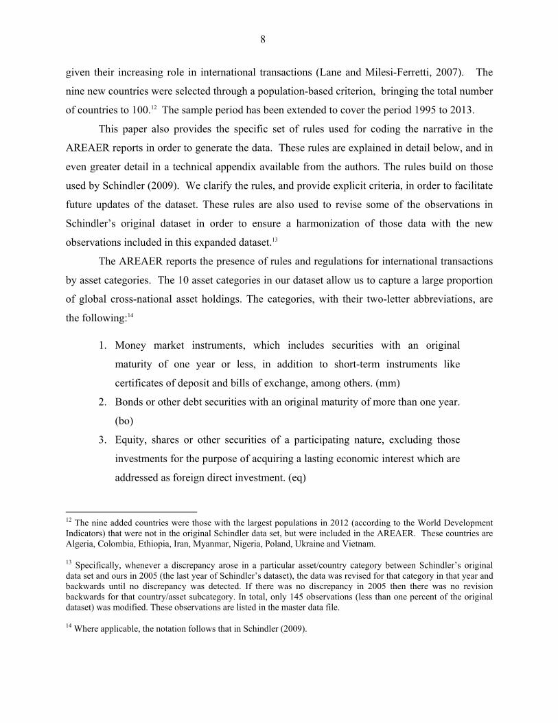
given their increasing role in international transactions (Lane and Milesi-Ferretti, 2007). The

nine new countries were selected through a population-based criterion, bringing the total number

of countries to 100.12 The sample period has been extended to cover the period 1995 to 2013.

This paper also provides the specific set of rules used for coding the narrative in the

AREAER reports in order to generate the data. These rules are explained in detail below, and in

even greater detail in a technical appendix available from the authors. The rules build on those

used by Schindler (2009). We clarify the rules, and provide explicit criteria, in order to facilitate

future updates of the dataset. These rules are also used to revise some of the observations in

Schindler’s original dataset in order to ensure a harmonization of those data with the new

observations included in this expanded dataset.13

The AREAER reports the presence of rules and regulations for international transactions

by asset categories. The 10 asset categories in our dataset allow us to capture a large proportion

of global cross-national asset holdings. The categories, with their two-letter abbreviations, are

the following:14

1. Money market instruments, which includes securities with an original

maturity of one year or less, in addition to short-term instruments like

certificates of deposit and bills of exchange, among others. (mm)

2. Bonds or other debt securities with an original maturity of more than one year.

(bo)

3. Equity, shares or other securities of a participating nature, excluding those

investments for the purpose of acquiring a lasting economic interest which are

addressed as foreign direct investment. (eq)

12 The nine added countries were those with the largest populations in 2012 (according to the World Development Indicators) that were not in the original Schindler data set, but were included in the AREAER. These countries are Algeria, Colombia, Ethiopia, Iran, Myanmar, Nigeria, Poland, Ukraine and Vietnam.

13 Specifically, whenever a discrepancy arose in a particular asset/country category between Schindler’s original data set and ours in 2005 (the last year of Schindler’s dataset), the data was revised for that category in that year and backwards until no discrepancy was detected. If there was no discrepancy in 2005 then there was no revision backwards for that country/asset subcategory. In total, only 145 observations (less than one percent of the original dataset) was modified. These observations are listed in the master data file.

14 Where applicable, the notation follows that in Schindler (2009).

9

4. Collective investment securities such as mutual funds and investment trusts.

(ci)

5. Financial credit and credits other than commercial credits granted by all

residents, including banks, to nonresidents, or vice versa. (fc)

6. Derivatives, which includes operations in rights, warrants, financial options

and futures, secondary market operations in other financial claims, swaps of

bonds and other debt securities, and foreign exchange without any other

underlying transaction. (de)

7. Commercial Credits for operations directly linked with international trade

transactions or with the rendering of international services. (cc)

8. Guarantees, Sureties and Financial Back-Up Facilities provided by residents

to nonresidents, and vice versa, which includes securities pledged for payment

or performance of a contract—such as warrants, performance bonds, and

standby letters of credit—and financial backup facilities that are credit

facilities used as a guarantee for independent financial operations. (gs)

9. Real Estate transactions representing the acquisition of real estate not

associated with direct investment, including, for example, investments of a

purely financial nature in real estate or the acquisition of real estate for

personal use. (re)

10. Direct investment accounts for transactions made for the purpose of

establishing lasting economic relations both abroad by residents and

domestically by nonresidents. (di)

The AREAER distinguishes across types of transactions according to the residency of the

buyer or the seller, and whether the transaction represents a purchase or a sale or issuance. For

five asset categories, Money Market, Bonds, Equities, Collective Investments and Derivatives,

there are four categories of transactions controls: two categories of controls on inflows, including

Purchase Locally by Non-Residents (plbn) and Sale or Issue Abroad by Residents (siar); and two

categories of controls on outflows, which are Purchase Abroad by Residents (pabr) and Sale or

Issue Locally by Non-Residents (siar). The Real Estate category includes the inflow transaction

category plbn and the outflow control transaction categories pabr and Sale Locally by Non-

Residents (slbn). There is only a broader classification of inflow controls or outflow controls for

10

the three categories of Financial Credits (fci and fco), Commercial Credits (cci and cco), and

Guarantees, Sureties and Financial Backup Facilities (gsi and gso). Direct Investment includes

the categories of controls on inflows (dii), controls on outflows (dio), and controls on the

Liquidation of Direct Investment (ldi) which captures controls on capital inflows or outflows

from the liquidation of direct investment abroad or domestically. Thus, in its most disaggregated

format, our dataset provides information on 32 transaction categories. Table 1 summarizes those

categories.

Table 1. Asset and Transaction Categories for Capital Control Measures Assets that Each Include Four Transaction Categories mm Money Market (Bonds with Maturity of 1 year or less) bo Bonds (Bonds with Maturity of greater than 1 year) eq Equities ci Collective Investments de Derivatives

Categories Inflow Controls: _plbn Purchase Locally By Non-Residents _siar Sale or Issue Abroad By Residents Outflow Controls: _pabr Purchase Abroad By Residents _siln Sale or Issue Locally By Non-Residents

Assets that Include Only Inflow (i) or Outflow (o) Categories gsi & gso Guarantees, Sureties & Financial Backup Facilities fci & fco Financial Credits cci & cco Commercial Credits Real Estate Re Real Estate

Categories Outflow _pabr Real Estate Purchase Abroad By Residents _slbn Sale Locally By Non-Residents Inflow _plbn Real Estate Purchase Locally By Non-Residents

Direct Investment dii Direct Investment Controls on Inflows dio Direct Investment Controls on Outflows ldi Direct Investment Controls on Liquidation The four series for each of the five categories of assets mm, bo, eq, ci, and de have the suffixes _plbn, _siar, _pabr or _siln. Real Estate is represented by the three series re_pabr, re_slbn and re_plbn. The suffixes for the three series gs, fc, and cc represent inflow or outflow controls (e.g., gsi and gso, respectively).

11

We use the narrative description in the AREAER to determine whether or not there are

restrictions on international transactions, with 1 representing the presence of a restriction and 0

representing no restriction.15 This requires a set of rules on interpreting the information presented

in these narratives. We formulated rules consistent with those used for the original Schindler

(2009) dataset, developing them when further clarification was warranted. The key points of

these rules are:16

1. The annual information from the AREAER reports comes with three columns;

the first listing the asset subcategory, the second containing a YES (that is, a

restriction is in place), a NO, or no entry, and the third including narrative

information. When coding each subcategory we first look at the information in

both columns two and three of the reports and follow these criteria:

i. If there is no narrative information in the third column we code on the

basis of the information in the second column where we assign a 0 for

NO and a 1 for YES.

ii. If there is information in the third column we code based on the

narrative information in that column.

2. A control is deemed to be in place when the narrative information alludes to a

transaction explicitly requiring “authorization,” “approval,” “permission,” or

“clearance” from a public institution. However, a requirement of “reporting,”

“registration,” or “notification” is not counted as constituting a control.

15 The AREAER narrative is limited to either n.r. or n.a. in about 2.8 percent of the cases in our data. The entry n.a. is used by the IMF “when it is unclear whether a particular category or measure exists – because pertinent information is not available at the time of publication.” (IMF, 2011: page ?) The entry n.r. is used when “members have provided the IMF staff with information that a category or an item is not regulated.” In addition, our dataset has the category d.n.e. that represents “does not exist” to document the cases where there is no information whatsoever, but this appears only 15 times in the entire dataset (0.03 percent of the dataset). The dataset available on line retains the n.r., n.a., and d.n.e. entries, but in the statistics presented in this paper we set to missing an entry with any of these three classifications.

16 A more detailed description of our rules and guiding principles is contained in the Technical Appendix.

12

3. A quantity restriction on any investment (e.g. in the form of “ceiling”) is

coded as a control. In addition, an explicit allusion to a restriction for

“prudential” considerations is deemed to be a control.

4. Restrictions on a particular asset that prevent capital flows from and into

specific countries on the basis of political or national security reasons are not

considered capital controls.

5. When there is a restriction specifically for transactions for only one sector

(except the financial system or for pension funds) and/or when that restriction

is for an area reserved for state control (such as defense, security, central

banking, etc.) that restriction is not categorized as a capital control. If, on the

other hand, the restriction does not specify which areas other than defense are

reserved for state control, then the restriction is categorized as a control.

Restrictions are counted as a capital control if they cover more than one sector

in which private entrepreneurship is common, and these restrictions are

deemed to have a macroeconomic impact.

There are a variety of ways to aggregate these data series in order to obtain a smaller set

of indicators than the full set of 32 categories presented in Table 1. The most basic aggregation

is to have indicators of inflow controls and outflow controls for the ten asset categories. This

does not require any aggregation for the asset categories of Commercial Credits, Financial

Credits or Guaranties, Sureties and Financial Backup Facilities since the dataset only includes

their inflow (cci, fci and gsi) and outflow (cco, fco and gso) categories, and the value of each of

these indicators will be either 0 or 1. We do not aggregate Direct Investment on Inflows,

Outflows and Controls on Liquidation of Direct Investment in this paper, but keep the three

categories separate, denoting them as dii, dio, and ldi, all of which will have values of either 0 or

1. In the case of Real Estate, there is only one inflow category (which we denote rei), but there

would need to be an aggregation of re_pabr and re_slbn to obtain a single, aggregate outflow

category (which we call reo).

The aggregation scheme that we follow to obtain a single outflow category for Real

Estate, as well as both an inflow indicator and an outflow indicator for the other five asset

categories that each have two inflow and outflow categories, is to construct indices that represent

the average of the inflow or outflow indicators. For each of these 11 asset categories, the

13

aggregate inflow index is the average of the 0 or 1 in Purchased Locally by Nonresidents and

Sale or Issue Abroad by Residents, and the aggregate outflow index is the average of the 0 or 1

in Purchased Abroad by Residents and Sale or Issue Locally by Non-Residents (or, for Real

Estate, Sale Locally by Non-Residents). Thus the values of mmi, mmo, boi, boo, eqi, eqo, cii,

cio, dei, deo and reo will be 0, ½ or 1.17 For these categories, one could interpret an entry of one

as representing greater intensity of controls than an entry of ½.

III. CHARACTERISTICS OF THE CAPITAL CONTROL INDICATORS

In this section, we present some characteristics of the capital control data. We begin by

considering the properties of inflow and outflow controls for the ten asset categories. We then

discuss aggregating these series into broader indicators that reflect the average level of controls

for the full set of assets, or for subsets consisting of two or more categories. We conclude this

section with an estimation of the correlation between our broad capital control indicator and two

other popular indicators of aggregate capital controls.

The dataset covers 100 countries over the period 1995 to 2013. The list of countries, by

World Bank Income Group, is presented in Table 2. As shown in that table, there are 42 high

income countries, 32 upper middle income countries, 18 lower middle income countries, and

eight low income countries.

This table also includes Klein’s (2012) classification of a country as Open, Gate or Wall.

There will be further discussion of this classification below, but the basic point is that an Open

country has virtually no capital controls on any asset category over the sample period, a Wall

country has pervasive controls across all, or almost all, categories of assets and a Gate country

uses capital controls episodically.

We begin by considering the prevalence of controls, by asset/direction categories (where

direction refers to whether the control is on inflows or outflows). The detailed nature of our data

set permits an examination of differences across these categories. These differences could be

important because the effects of policies may vary depending upon whether controls are targeted

towards inflows or outflows of particular classes of assets. Broad indicators of capital controls

17 When there is a missing value in one of the two inflow or outflow subcategories (see footnote 12), we score the aggregate inflow or outflow entry with the value taken by the remaining subcategory.

14

that do not distinguish across asset categories, or even between controls on inflows and controls

on outflows, will mask potentially important variations in the types of controls.

Figure 1 shows the prevalence of controls across 20 asset/direction categories. In this

figure, no distinction is made between a value of ½ and 1; instead, each is treated equally as a

control. The prevalence of controls ranges from 18 percent of observations (for liquidation of

direct investment), to 25 percent (for inflow controls on Guarantees, Sureties and Financial

Backup Facilities) to 50 percent or greater (for inflow controls on Real Estate and outflow

controls on Money Market Instruments, Bonds, Equities, Collective Investments, and

Derivatives). The figure also demonstrates that, with the exceptions of Real Estate and Direct

Investment, there is a higher prevalence of controls on outflows than on inflows.

0

.05

.1

.15

.2

.25

.3

.35

.4

.45

.5

.55

Pro

port

ion

with

Co

ntro

ls

m

mi

mm

obo

ibo

oeq

ieq

o cii cio deide

o rei

reo fci fc

o cci

cco gs

igs

o dii dio ldi

Asset Category and Direction (Inflow (i) or Outflow (o)) of Restriction

By Asset Category and Direction of RestrictionFigure 1: Proportion of Observations With Controls

15

Table 2. Countries In Data Set, By Income Groups, With Open/Gate/Wall Category

High (42) Upper Middle (26) Lower Middle & Low (32) Australia Gate Algeria Wall Bangladesh* Gate Austria Open Angola Wall Bolivia Gate Bahrain Gate Argentina Gate Burkina Faso* Gate Belgium Open Brazil Gate Cote d'Ivoire Wall Brunei Darussalam Open Bulgaria Gate Egypt Open Canada Open China Wall El Salvador Open Chile Gate Colombia Gate Ethiopia* Gate Cyprus Gate Costa Rica Open Georgia Open Czech Republic Gate Dominican Republic Gate Ghana Gate Denmark Open Ecuador Gate Guatemala Open Finland Open Hungary Gate India Wall France Open Iran Gate Indonesia Gate Germany Gate Jamaica Gate Kenya* Gate Greece Open Kazakhstan Gate Kyrgyz Republic Gate Hong Kong Open Lebanon Gate Moldova Gate Iceland Gate Malaysia Wall Morocco Wall Ireland Open Mauritius Open Myanmar* Gate Israel Gate Mexico Gate Nicaragua Open Italy Open Panama Open Nigeria Gate Japan Open Peru Open Pakistan Wall Korea Gate Romania Gate Paraguay Open Kuwait Gate South Africa Gate Philippines Wall Latvia Open Thailand Gate Sri Lanka Wall Malta Gate Tunisia Wall Swaziland Wall Netherlands Open Turkey Gate Tanzania* Wall New Zealand Open Venezuela Gate Togo* Wall Norway Open Uganda* Gate Oman Open Ukraine Wall Poland Gate Uzbekistan Wall Portugal Gate Vietnam Gate Qatar Open Yemen Open Russia Gate Zambia Open Saudi Arabia Gate

* = Low Income rather than Lower Middle Income

Singapore Open Slovenia Gate Spain Open Sweden Open Switzerland Gate U.A.E. Gate United Kingdom Open United States Open Uruguay Open Open (36) / Gate (48) / Wall (16) 24 / 18 / 0 4 / 17 / 5 8 / 13/ 11 Note: Following Klein (2012), “Open” (“Walls”) countries have, on average, capital controls on less than 10 percent (more than 70 percent) of their transactions subcategories over the sample period and do not have any years in which controls are on more than 20 percent (less than 60 percent) of their transaction subcategories. “Gate” countries are neither Walls nor Open.

16

A more detailed analysis by asset/direction category is presented in Table 3. The first set

of columns shows the average control values (0, ½ or 1) for those eleven asset/direction

categories that have two components for inflows or outflows, and the second set of columns

shows the number of cases where controls are absent or present for the ten asset/direction

categories that have only one component each for inflows and outflows. The final row of the

second column shows that overall, 40 percent of the observations represent cases in which there

are capital controls. For the asset/direction categories that can take the value 0, ½ or 1, there are

more observations of 1 than of ½ (the difference is 26 percent of observations versus 20 percent).

Table 3. Prevalence of Controls, 100 Countries, 1995 – 2013, by Asset Sub-Categories

0 0.5 1 Total Pr. Cntrl

0 1 Total Pr. Cntrl

mmi 1,143 346 388 1,877 0.39 fci 1,205 685 1,890 0.36 mmo 917 367 589 1,873 0.51 fco 1,119 767 1,886 0.41 boi* 980 378 327 1,685 0.42 cci 1,337 546 1,883 0.29 boo* 807 356 517 1,680 0.52 cco 1,225 644 1,869 0.34 eqi 1,024 459 399 1,882 0.46 gsi 1,384 471 1,855 0.25 eqo 914 388 584 1,886 0.52 gso 1,227 631 1,858 0.34 cii 1,152 360 335 1,847 0.38 dii 1,121 779 1,900 0.41 cio 892 398 577 1,867 0.52 dio 1,246 625 1,871 0.33 dei 1,073 219 452 1,744 0.38 ldi 1,546 334 1,880 0.18 deo 890 310 585 1,785 0.50 rei 828 1,034 1,862 0.55 reo 1,084 395 388 1,867 0.42 Total 23,469 15,134† 38,603 0.40 Pr. Cntrl. = Proportion of observations with controls (i.e. either ½ or 1) _i = control on inflows. _o = control on outflows mm – Money Market Instruments (Debt instruments with maturity 1 year or less) bo – Bonds (Debt instruments with maturity greater than 1 year) eq – Equities ci – Collective Investments de – Derivatives re – Real Estate fc – Financial Credits cc – Commercial Credits gs – Guaranties & Sureties di – Direct Investment ldi – liquidation of direct investment *Data on Bonds available 1997-2013 † This entry represents number of values equal to 0.5 or 1.

The detailed nature of our dataset enables us to consider, along with differences in the

prevalence of controls across asset/direction categories, the correlation of controls across these

categories.18 This is of interest for a number of reasons, including how governments choose to

18 The correlations are across all observations, that is, across all pairs x(t), y(t), where x and y represent asset/direction categories and t represents the time period. Correlations will be missing if the variance of an indicator is zero, but, in practice, there are relatively few instances of this, even among the Open and Walls

(continued…)

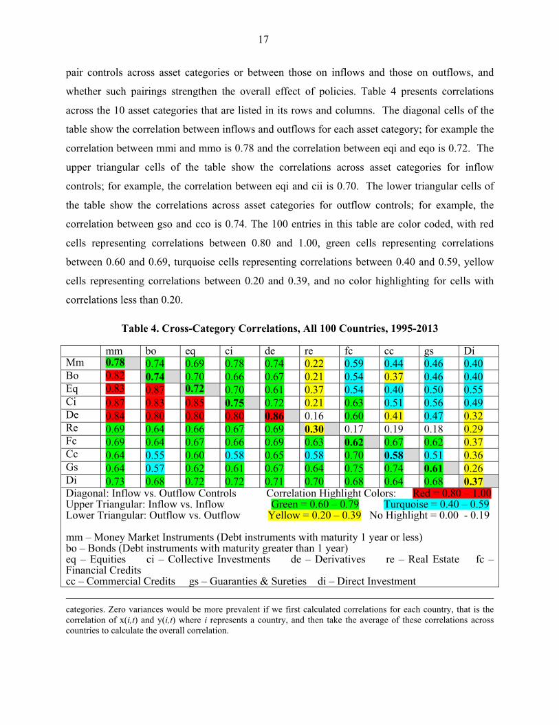
17

pair controls across asset categories or between those on inflows and those on outflows, and

whether such pairings strengthen the overall effect of policies. Table 4 presents correlations

across the 10 asset categories that are listed in its rows and columns. The diagonal cells of the

table show the correlation between inflows and outflows for each asset category; for example the

correlation between mmi and mmo is 0.78 and the correlation between eqi and eqo is 0.72. The

upper triangular cells of the table show the correlations across asset categories for inflow

controls; for example, the correlation between eqi and cii is 0.70. The lower triangular cells of

the table show the correlations across asset categories for outflow controls; for example, the

correlation between gso and cco is 0.74. The 100 entries in this table are color coded, with red

cells representing correlations between 0.80 and 1.00, green cells representing correlations

between 0.60 and 0.69, turquoise cells representing correlations between 0.40 and 0.59, yellow

cells representing correlations between 0.20 and 0.39, and no color highlighting for cells with

correlations less than 0.20.

Table 4. Cross-Category Correlations, All 100 Countries, 1995-2013

mm bo eq ci de re fc cc gs DiMm 0.78 0.74 0.69 0.78 0.74 0.22 0.59 0.44 0.46 0.40 Bo 0.82 0.74 0.70 0.66 0.67 0.21 0.54 0.37 0.46 0.40 Eq 0.83 0.87 0.72 0.70 0.61 0.37 0.54 0.40 0.50 0.55 Ci 0.87 0.83 0.85 0.75 0.72 0.21 0.63 0.51 0.56 0.49 De 0.84 0.80 0.80 0.80 0.86 0.16 0.60 0.41 0.47 0.32 Re 0.69 0.64 0.66 0.67 0.69 0.30 0.17 0.19 0.18 0.29 Fc 0.69 0.64 0.67 0.66 0.69 0.63 0.62 0.67 0.62 0.37 Cc 0.64 0.55 0.60 0.58 0.65 0.58 0.70 0.58 0.51 0.36 Gs 0.64 0.57 0.62 0.61 0.67 0.64 0.75 0.74 0.61 0.26 Di 0.73 0.68 0.72 0.72 0.71 0.70 0.68 0.64 0.68 0.37 Diagonal: Inflow vs. Outflow Controls Correlation Highlight Colors: Red = 0.80 – 1.00Upper Triangular: Inflow vs. Inflow Green = 0.60 – 0.79 Turquoise = 0.40 – 0.59 Lower Triangular: Outflow vs. Outflow Yellow = 0.20 – 0.39 No Highlight = 0.00 - 0.19 mm – Money Market Instruments (Debt instruments with maturity 1 year or less) bo – Bonds (Debt instruments with maturity greater than 1 year) eq – Equities ci – Collective Investments de – Derivatives re – Real Estate fc – Financial Credits cc – Commercial Credits gs – Guaranties & Sureties di – Direct Investment

categories. Zero variances would be more prevalent if we first calculated correlations for each country, that is the correlation of x(i,t) and y(i,t) where i represents a country, and then take the average of these correlations across countries to calculate the overall correlation.

18

The table shows that the correlation between inflow controls and outflow controls for a

given asset tends to be high. The highest correlation between inflow and outflow controls is for

Derivatives (86 percent) and the lowest is for Direct Investment (37 percent) and Real Estate

(30 percent). This result echoes that obtained by Fernández, Rebucci and Uribe (2014), who

show that the cyclical components of capital controls on inflows and outflows are positively

correlated. The correlation between asset categories, for both inflow controls and outflow

controls, is highest among Money Market Instruments, Bonds, Equities, Collective Investments,

and Derivatives. The lowest correlations are found for inflow controls between Real Estate and

each of the other nine categories of assets. More broadly, the correlations are higher among the

asset categories for outflow controls than for inflow controls.

Countries that had almost no controls for any category over the entire sample period, as

well as countries that had controls on virtually all assets in every year, will contribute to larger

values of the correlations in Table 4. We call these Open countries and Wall countries,

respectively, following Klein (2012). In particular, the 36 countries in the Open category (which

includes 24 of the 42 High Income countries) each had capital controls on less than 15 percent of

their asset/direction categories over the sample period and had no year in which capital controls

were in place on more than 25 percent of the categories. The 16 countries in the Wall category

(which includes 11 of the 26 Lower Middle Income and Low Income countries) each had

controls on at least 70 percent of their asset/transaction categories and had no year in which

capital controls were in place on less than 60 percent of the categories. The 48 countries that are

neither Open nor Wall are classified as Gate countries. As mentioned above, Table 1 notes the

classification of each country in terms of these three categories.

Table 5A presents the correlations across asset/direction categories for the 48 Gate

countries and Table 5B presents these correlations for the 52 Open and Wall countries. As

expected, the correlations for the Gate countries are lower than those of the other countries, with

only one greater than 80 percent (red cell) and 40 less than 40 percent (yellow cells, and cells

without highlighting). In contrast, all the correlations in Table 5B among outflows are greater

than 80 percent, and the majority of those among inflows (but for correlations with real estate)

greater than 60 percent, with a fifth of the inflow restriction correlations greater than 80 percent.

19

Table 5A. Cross-Category Correlations, 47 Gate Countries, 1995-2013

mm bo Eq Ci De re fc cc gs dimm 0.69 0.65 0.55 0.66 0.69 0.03 0.47 0.27 0.26 0.29 bo 0.71 0.58 0.55 0.46 0.54 0.01 0.30 0.11 0.24 0.23 eq 0.67 0.81 0.55 0.51 0.43 0.22 0.30 0.10 0.27 0.44 ci 0.77 0.75 0.70 0.60 0.57 -0.01 0.46 0.33 0.35 0.41 de 0.76 0.70 0.63 0.64 0.79 -0.03 0.43 0.15 0.18 0.19 re 0.57 0.43 0.44 0.52 0.54 0.08 -0.02 -0.07 0.01 0.24 fc 0.50 0.42 0.41 0.45 0.51 0.43 0.48 0.59 0.43 0.27 cc 0.39 0.23 0.24 0.23 0.38 0.33 0.55 0.46 0.36 0.27 gs 0.41 0.29 0.31 0.31 0.46 0.41 0.65 0.60 0.44 0.17 di 0.54 0.50 0.51 0.54 0.51 0.56 0.52 0.38 0.50 0.22 Diagonal: Inflow vs. Outflow Controls Correlation Highlight Colors: Red = 0.80 – 1.00Upper Triangular: Inflow vs. Inflow Green = 0.60 – 0.79 Turquoise = 0.40 – 0.59 Lower Triangular: Outflow vs. Outflow Yellow = 0.20 – 0.39 No Highlight = 0.00 - 0.19 mm – Money Market Instruments (Debt instruments with maturity 1 year or less) bo – Bonds (Debt instruments with maturity greater than 1 year) eq – Equities ci – Collective Investments de – Derivatives re – Real Estate fc – Financial Credits cc – Commercial Credits gs – Guaranties & Sureties di – Direct Investment

Table 5B. Cross-Category Correlations, 53 Open and Wall Countries, 1995-2013

mm bo Eq Ci De re fc cc gs dimm 0.83 0.83 0.82 0.90 0.79 0.37 0.71 0.60 0.70 0.47 bo 0.89 0.86 0.83 0.85 0.80 0.37 0.78 0.63 0.73 0.53 eq 0.93 0.91 0.85 0.88 0.77 0.48 0.77 0.70 0.75 0.63 ci 0.94 0.87 0.95 0.86 0.86 0.40 0.78 0.68 0.77 0.55 de 0.88 0.87 0.91 0.87 0.93 0.31 0.76 0.67 0.73 0.41 re 0.81 0.81 0.84 0.80 0.83 0.47 0.33 0.43 0.34 0.31 fc 0.84 0.81 0.88 0.84 0.84 0.80 0.76 0.74 0.82 0.43 cc 0.86 0.82 0.90 0.87 0.89 0.81 0.84 0.70 0.69 0.43 gs 0.84 0.80 0.88 0.86 0.87 0.85 0.85 0.87 0.79 0.38 di 0.90 0.85 0.90 0.87 0.90 0.83 0.83 0.91 0.87 0.50Diagonal: Inflow vs. Outflow Controls Correlation Highlight Colors: Red = 0.80 – 1.00Upper Triangular: Inflow vs. Inflow Green = 0.60 – 0.79 Turquoise = 0.40 – 0.59 Lower Triangular: Outflow vs. Outflow Yellow = 0.20 – 0.39 No Highlight = 0.00 - 0.19 mm – Money Market Instruments (Debt instruments with maturity 1 year or less) bo – Bonds (Debt instruments with maturity greater than 1 year) eq – Equities ci – Collective Investments de – Derivatives re – Real Estate fc – Financial Credits cc – Commercial Credits gs – Guaranties & Sureties di – Direct Investment

20

Correlations in controls for the subset of Gate countries are a better indicator of the

manner in which countries pair controls used episodically than the correlations for the full set of

countries. The highest correlations for the Gate countries are those between outflow controls on

Money Market Instruments, Bonds, Equities, Collective Investments and Derivatives. The lowest

correlations are those for inflow controls with Commercial Credits, and Real Estate. These

patterns of correlations will inform our decisions on which asset categories to use when

constructing aggregate capital control indices, which is the topic of the next section.

IV. AGGREGATE INDICATORS

The correlations presented in Tables 4 and 5 are based on disaggregated asset/direction

categories (with averages used for the categories that have two components for either inflows or

outflows). In many instances it may be desirable to have a more aggregated indicator. For

instance, one might be interested in studying the intensity with which capital controls are

applied. By tracking variations across asset categories, directions of transactions, and time,

aggregate indices capture a form of intensity of restrictions on capital movements across borders.

Indeed, Fernández, Uribe and Rebucci (2014) show that an aggregate index of controls on capital

inflows captures well the evolution of actual tax rates on capital inflows in the emblematic case

of Brazil in the late 2000s. In this section we present a number of aggregate indicators and use

them to demonstrate some characteristics of the capital control data.

An aggregate of the capital control indicators is important for presenting the evolution of

capital controls over time; a graph of the 32 disaggregated capital control categories would be

hopelessly muddled. Therefore, we first calculate two broad indicator of the stance of each

country towards capital controls, one as the average value controls on inflows for the 10 asset

categories in each year,

, ∑ , ,

and another as the controls on outflows,

, ∑ , ,

21

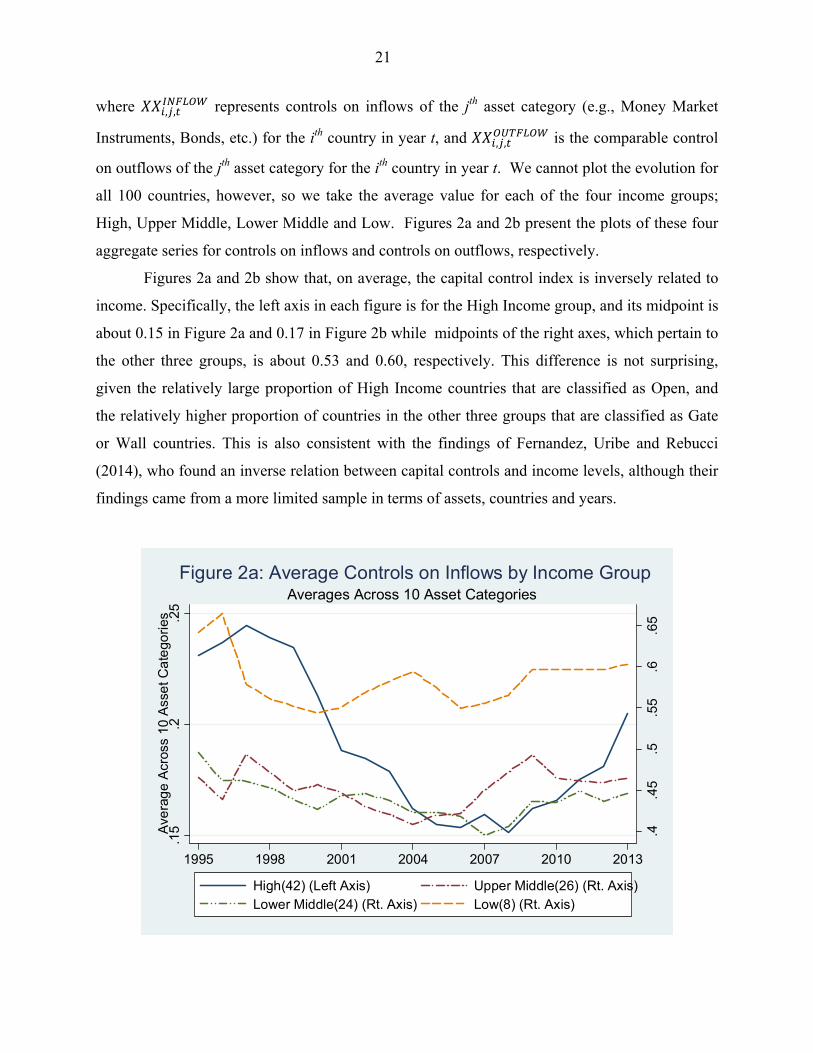
where , , represents controls on inflows of the jth asset category (e.g., Money Market

Instruments, Bonds, etc.) for the ith country in year t, and , , is the comparable control

on outflows of the jth asset category for the ith country in year t. We cannot plot the evolution for

all 100 countries, however, so we take the average value for each of the four income groups;

High, Upper Middle, Lower Middle and Low. Figures 2a and 2b present the plots of these four

aggregate series for controls on inflows and controls on outflows, respectively.

Figures 2a and 2b show that, on average, the capital control index is inversely related to

income. Specifically, the left axis in each figure is for the High Income group, and its midpoint is

about 0.15 in Figure 2a and 0.17 in Figure 2b while midpoints of the right axes, which pertain to

the other three groups, is about 0.53 and 0.60, respectively. This difference is not surprising,

given the relatively large proportion of High Income countries that are classified as Open, and

the relatively higher proportion of countries in the other three groups that are classified as Gate

or Wall countries. This is also consistent with the findings of Fernandez, Uribe and Rebucci

(2014), who found an inverse relation between capital controls and income levels, although their

findings came from a more limited sample in terms of assets, countries and years.

.4.4

5.5

.55

.6.6

5

.15

.2.2

5A

vera

ge

Acr

oss

10 A

sse

t Ca

tego

ries

1995 1998 2001 2004 2007 2010 2013

High(42) (Left Axis) Upper Middle(26) (Rt. Axis)Lower Middle(24) (Rt. Axis) Low(8) (Rt. Axis)

Averages Across 10 Asset CategoriesFigure 2a: Average Controls on Inflows by Income Group

22

Another distinction across the income groups is the pattern of average capital controls

over time. The High Income group of countries has a large decrease in its average from about

0.20 for inflows and 0.22 for outflows in the first years of the sample period to less than 0.10 in

2008 for inflows and 0.12 in 2004 for outflows before rising again in the subsequent years. The

Low Income countries as a group also see a large decline in their average inflow and outflow

controls in the first years of the sample period, and then an increase, especially in average

controls on outflows. The range of the averages across time for both inflow controls and outflow

controls for the two Middle Income groups is lower than the other groups, and the averages

themselves are lower than the Low Income group but more than twice as high as those for the

High Income group.

The aggregate indicators used to generate Figures 2a and 2b show some differences

between controls on inflows and controls on outflows. We further consider the relationship

between inflow controls and outflow controls by calculating, for each country, its average

controls on inflows and outflows over the full sample period, KCINFLOWi and KCOUTFLOW

i,

respectively. These are defined as

.4.5

.6.7

.8

.12

.14

.16

.18

.2.2

2A

vera

ge

Acr

oss

10 A

sse

t Ca

tego

ries

1995 1998 2001 2004 2007 2010 2013

High(42) (Left Axis) Upper Middle(26) (Rt. Axis)Lower Middle(24) (Rt. Axis) Low(8) (Rt. Axis)

Averages Across 10 Asset CategoriesFigure 2b: Average Controls on Outflows by Income Group

23

∑ ∑ , ,

∑ ∑ , , .

Figure 3 presents the scatterplots of these country-by-country indicators (along with a 45-

degree line), with the left panel representing the 42 High income countries and the right panel

representing the 58 Medium and Low Income countries. The sizes of the bubbles in these figures

reflect the number of countries in a small range.

The two panels of this figure show a somewhat higher prevalence of outflow controls

than of inflow controls, consistent with the statistics in Table 3 and Figure 1. Figure 3 illustrates

that the difference in the prevalence of inflow and outflow controls is more pronounced for the

Medium and Lower Income countries than for the High Income countries. The two panels of

24 Open

Poland

0.2

5.5

.75

1In

flow

Con

trol

s

0 .25 .5 .75 1Outflow Controls

42 High Income Countries16 Closed

12 Open

Myanmar0

.25

.5.7

51

Inflo

w C

ontr

ols

0 .25 .5 .75 1Outflow Controls

58 Medium & Low Income Countries

Countries' Average Values for all Ten Assets, 1995 - 2012Figure 3: Inflow Controls vs. Outflow Controls

24

Figure 3 also show that there is a relatively high correlation of inflow and outflow controls on a

country-by-country basis (for both sets of countries, the correlation is about 0.8). This is

necessarily the case for the 36 Open countries and, to a somewhat lesser extent, for the 16 Wall

countries.

Figures 2 and 3 use aggregates either across sets of countries for each year or across time

for each country. In some cases we may want to take advantage of the detailed nature of the data

set and have an aggregate indicator based on a subset of assets; for example, Klein and

Shambaugh (2015) use an indicator that includes only Money Market Instruments and Bonds in

their analysis of interest parity as well as another indicator that includes those asset categories

plus Equities, Collective Investment and Financial Credits.

More generally, with any aggregate we would want to consider the benefit of having a

single measure against the cost of masking information by combining possibly disparate series.

An aggregate indicator will be more representative of its constituent series if the series are more

highly correlated with each other. For example, an aggregate indicator averaging the inflow and

outflow series for Derivatives is more representative of its two constituent parts than one that

averages the inflow and outflow indicators of Real Estate since the correlation of the former is

0.86 and that of the latter is 0.30. Likewise, an aggregate of the outflow controls for Money

Market Instruments, Bonds, Equities and Collective Investments would be one that is relatively

representative of each of these separate categories since each of the six pairwise correlations is

greater than 80 percent, while the broadening of this aggregate to include controls on

Commercial Credits would be less representative since the correlations of that category with the

other four range from 55 percent to 64 percent.

We begin by examining the correlation between the average of inflows and outflows of a

single asset with that of an average of an aggregate of the inflows and outflows of the other nine

assets. Table 6 presents this set of ten statistics. The table shows that controls on Real Estate,

Commercial Credits, Direct Investment, and Guarantees, Sureties, and Financial Backup

Facilities are least correlated with the aggregate of the respective nine remaining categories

while the correlation of Money Market Instruments, Collective Investments, Derivatives and

Equities are most highly correlated.

25

Table 6. Correlation between Nine-Asset Aggregate Capital Controls and Excluded Asset Category

Excluded Asset mm bo eq Fc ci de re cc gs di Correlation 0.87 0.83 0.87 0.83 0.88 0.87 0.61 0.71 0.79 0.77Entries represent the correlations between an aggregate 9-Asset Capital Flow Measure (both inflow and outflow controls) that exclude the asset category in listed in the column head, and that excluded asset.

We next consider a set of nested aggregate indicators that differ by the number of

component assets (again, each asset series represents the average of inflow and outflow

controls). All 10 assets are included in the broadest indicator, KC10i,t, which is the average of

the inflow and outflow indicators above,

10 , ∑ , , ∑ , ,

The series KC9i,t excludes direct investment, both because it is less correlated with the other

assets than almost any other series and because controls on direct investment often reflect non-

economic considerations. The series KC5i,t includes Money Market Instruments, Bonds, Equities,

Collective Investments, and Derivatives, five series that are relatively highly correlated. The

narrowest category, KC2i,t, includes only controls on fixed income assets, Money Market

Instruments and Bonds.

Table 7 presents the correlations across these categories for the full set of countries (the

six upper triangular elements of the table) and the Gate countries only (the six lower triangular

elements) for these four aggregate indicators. The correlations are very high for the full set of

countries, with a range from 0.924 (for the correlation between KC10 and KC2) to 0.995 (for the

correlation between KC9 and KC10). The correlations among these aggregates for the Gate

countries are, naturally, lower than the respective correlations for the full set of countries, and

there is also a greater range of values. For example, the correlation between the two-asset and

10-asset indicators is 0.873. In contrast, the difference in the correlation of the two-asset and

five-asset indicators between the full sample (0.971) and the sample of Gate countries (0.953) is

not nearly as large. Thus, there could be differences in the estimated effect of capital controls in

an analysis in which the identification depends upon the pattern of controls for Gates countries.

26

Table 7. Correlations among Aggregate Capital Controls Measures

KC10 KC9 KC5 KC2 KC10 0.995 0.954 0.924 KC9 0.992 0.958 0.928 KC5 0.901 0.910 0.971 KC2 0.873 0.877 0.953 KC10: Average of Inflows and Outflows for mm, bo, eq, ci, de, re fc, cc, gs, di. KC9: Average of Inflows and Outflows for mm, bo, eq, ci, de, re fc, cc, gs (all but di). KC5: Average of Inflows and Outflows for mm, bo, eq, ci, de. KC2: Average of Inflows and Outflows for mm, bo. Upper triangular elements show correlations among all 100 countries. Lower triangular elements show correlations among 48 Gate countries.

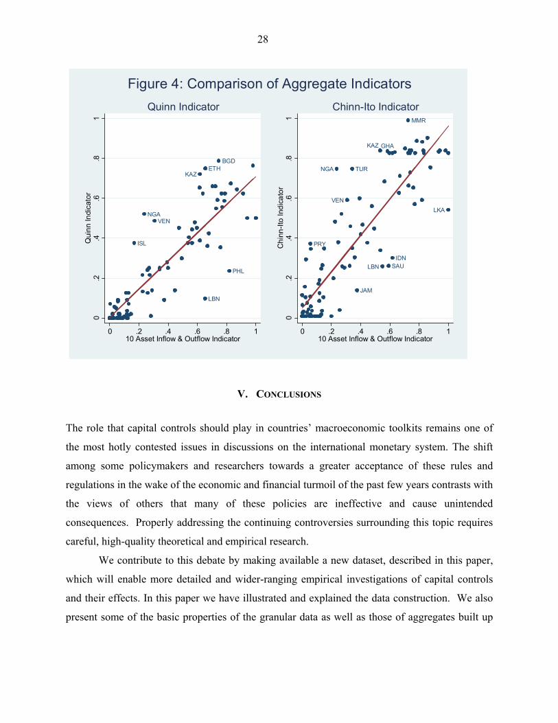
We conclude this section by considering the relationship between the average for each

country of our broadest indicator of capital controls, KC10i and the average, over the same time

periods, of two popular measures of aggregate capital controls that have been used in empirical

research. The index developed by Quinn (1997) attempts to capture the intensity of enforcement

of controls on both the capital account and the current account. As in the present study, Quinn

derives an index of capital controls from the narrative portion of the AREAER reports. To assess

the severity of the restrictions on capital flows, Quinn’s index uses a five-point scale at the

granular level. However, his index does not distinguish between capital controls on inflows and

capital controls on outflows. For purposes of comparison to our aggregate index, in the analysis

below we convert his capital account index to the range [0,1] in which, as with our index, larger

values represent more restrictions on capital account transactions. The Chinn-Ito index (first

presented in Chinn and Ito, 2006) takes the first principal component of the AREAER summary

binary codings of controls relating to current account transactions, capital account transactions,

the existence of multiple exchange rates, and the requirements of surrendering export proceeds.

As with the Quinn index, we convert this index to one with the range [0,1] in which larger values

represent more restrictions, to facilitate comparison with our index.

27

We regress the average value for each country of each of these two indices over the

sample period on the average value for each country of our broad indicator of capital account

controls, KC10i.19 These estimates, with the standard errors given in parentheses, are

0.004 . 0.71 . 10 0.77; 90

0.049 . 0.91 . 10 0.77; 99.

Plots of the regression lines, and the scatter plots of the points, are presented in the two panels of

Figure 4. We identify the country associated with each point for which the absolute value of the

regression error is greater than 0.25 for the regression for the Quinn indicator, and 0.20 for the

Chinn-Ito regression.

In both of these regressions, the coefficient on KC10i is significantly different from zero

at very high levels of confidence. But the more relevant test is whether these coefficients are

significantly different from 1. The t-statistic for this test in the regression with the Chinn-Ito

indicator is 1.71 and the t-statistic for the Quinn regression is 7.21. Thus, the null hypothesis

that the coefficients equal 1 can be rejected at the 95 percent level of confidence in both cases,

but not at the 90 percent level of confidence in the case of the Chinn-Ito indicator.

19 The average values of KC10i used in the regressions are calculated using annual data only for those countries that have data for the Quinn and the Chinn-Ito indices in the respective years (the averages KC10i are different for the Quinn and Chinn-Ito regressions since these two indices have different country coverage in each year). The sample period used to calculate these averages is 1995 to 2012.

28

V. CONCLUSIONS

The role that capital controls should play in countries’ macroeconomic toolkits remains one of

the most hotly contested issues in discussions on the international monetary system. The shift

among some policymakers and researchers towards a greater acceptance of these rules and

regulations in the wake of the economic and financial turmoil of the past few years contrasts with

the views of others that many of these policies are ineffective and cause unintended

consequences. Properly addressing the continuing controversies surrounding this topic requires

careful, high-quality theoretical and empirical research.

We contribute to this debate by making available a new dataset, described in this paper,

which will enable more detailed and wider-ranging empirical investigations of capital controls

and their effects. In this paper we have illustrated and explained the data construction. We also

present some of the basic properties of the granular data as well as those of aggregates built up

BGDETH

ISL

KAZ

LBN

NGA

PHL

VEN

0.2

.4.6

.81

Qui

nn

Indi

cato

r

0 .2 .4 .6 .8 110 Asset Inflow & Outflow Indicator

Quinn Indicator

GHA

IDN

JAM

KAZ

LBN

LKA

MMR

NGA

PRY

SAU

TUR

VEN

0.2

.4.6

.81

Ch

inn

-Ito

Ind

ica

tor

0 .2 .4 .6 .8 110 Asset Inflow & Outflow Indicator

Chinn-Ito Indicator

Figure 4: Comparison of Aggregate Indicators

29

from the individual data series. Our hope is that this dataset proves useful in moving forward our

understanding of this important topic.

30

VI. REFERENCES

Bhagwati, J. 1998. “The Capital Myth: The Difference between Trade in Widgets and Trade in

Dollars.” Foreign Affairs 77: 7–12.

Benigno, G. et al. 2014. “Optimal Capital Controls and Exchange Rate Policy? A Pecuniary

Externality Perspective.” CEPR Discussion Paper 9936. London, United Kingdom:

Centre for Economic Policy Research.

Bianchi, J. 2011. “Overborrowing and Systemic Externalities in the Business Cycle.” American

Economic Review 101(7): 3400–3426.

Binici, M., M. Schindler and M. Hutchison. 2010. “Controlling Capital? Legal Restrictions and

the Asset Composition of International Financial Flows.” Journal of International Money

and Finance 29(4): 666–684.

Chinn, M.D., and Hiro Ito. 2006. “What Matters for Financial Development? Capital Controls,

Institutions, and Interactions.” Journal of Development Economics 81(1): 163-192.

----. 2008. “A New Measure of Financial Openness.” Journal of Comparative Policy Analysis

10: 309–22.

De Gregorio, J., S. Edwards and R. Valdés. 2000. “Controls on Capital Inflows: Do They

Work?” Journal of Development Economics 69: 59-83.

Dornbusch, Rudiger. 1998. “Capital Controls: An Idea Whose Time is Gone.” Cambridge,

United States: Massachusetts Institute of Technology. Mimeographed document.

Farhi, E., and I. Werning. 2012. “Dealing with the Trilemma: Optimal Capital Controls with

Fixed Exchange Rates.” NBER Working Paper 18199. Cambridge, United States:

National Bureau of Economic Research.

Fernández, A., A. Rebucci and M. Uribe. 2014. “Are Capital Controls Countercylical?” New

York, United States: Columbia University. Mimeographed document.

Forbes, K. 2007. “One Cost of Chilean Capital Controls: Increased Financial Constraints for

Smaller Traded Firms.” Journal of International Economics 71: 294–323.

Forbes, K. et al. 2012. “Bubble Thy Neighbor: Direct and Spillover Effects of Capital Controls.”

NBER Working Paper 18052. Cambridge, United States: National Bureau of Economic

Research.

31

Grilli, V., and G-M. Milesi-Ferretti. 1995. “Economic Effects and Structural Determinants of

Capital Controls.” IMF Staff Papers 42(3): 517–51.

IMF Strategy, Policy and Review Department. 2011. “Recent Experiences in Managing Capital

Inflows: Cross-Cutting Themes and Possible Policy Framework.” Washington, DC,

United States: International Monetary Fund. Available at:

http://www.imf.org/external/np/pp/eng/2011/021411a.pdf

Jeanne, O. 2012. “Capital Flow Management.” American Economic Review Papers and

Proceedings 102(3): 203–06.

Jeanne, O., A. Subramanian and J. Williamson. 2012. Who Needs to Open the Capital Account?

Washington, DC, United States: Peterson Institute for International Economics.

Keynes, J.M. 1920. The Economic Consequences of the Peace. New York, United States:

Harcourt, Brace and Howe.

Klein, M.W. 2012. “Capital Controls: Gates versus Walls.” Brookings Papers on Economic

Activity 2012 (Fall): 317-355.

Klein, M.W. and J. Shambaugh. 2015. “Rounding the Corners of the Policy Trilemma: Sources

of Monetary Policy Autonomy.” Forthcoming in American Economic Journal:

Macroeconomics.

Korinek, A. 2010. “Regulating Capital Flows to Emerging Markets: An Externality View.”

College Park, United States: University of Maryland. Mimeographed document.

Lane, P., and G-M. Milesi-Ferretti. 2007. “The External Wealth of Nations Mark II.” Journal of

International Economics 73: 223-250.

Miniane, J. 2004. “A New Set of Measures on Capital Account Restrictions.” IMF Staff Papers

51: 276–308.

Ostry, J. et al. 2010. “Capital Inflows: The Role of Controls.” IMF Staff Position Note

SPN/10/04. Washington, DC, United States: International Monetary Fund.

Ostry, J. et al. 2011. “Capital Controls: When and Why.” IMF Economic Review 59(3): 562-580.

Prati, A., M. Schindler and P. Valenzuela. 2012. “Who Benefits from Capital Account

Liberalization? Evidence from Firm-Level Credit Ratings Data.” Journal of International

Money and Finance 31(6): 1649–1673.

Quinn, D. 1997. “The Correlates of Change in International Financial Regulation.” American

Political Science Review 91(3): 531–51.

32

Quinn, D., M. Schindler and A.M. Toyoda. 2011. “Assessing Measures of Financial Openness

and Integration.” IMF Economic Review 59(3): 488-522.

Rey, H. 2014. “Dilemma not Trilemma: The Global Financial Cycle and Monetary

Independence.” In: Global Dimensions of Unconventional Monetary Policy: A

Symposium Sponsored By the Federal Reserve Bank of Kansas City, Jackson Hole,

Wyoming, August 22-24, 2013. Kansas City, United States: Federal Reserve Bank.

Rodrik, D. 1998. “Who Needs Capital-Account Convertibility?” In: S. Fischer et al., editors.

Should the IMF Pursue Capital Account Convertibility? Essays in International Finance

207. Princeton, United States: Princeton University, Department of Economics,

International Finance Section.

Rogoff, K.S. 2002. “Rethinking Capital Controls: When Should We Keep an Open Mind?”

Finance and Development 39(4): 55-56.

Schindler, M. 2009. “Measuring Financial Integration: A New Data Set.” IMF Staff Papers

56(1): 222–38.

Schmitt-Grohé, S., and M. Uribe. 2012. “Prudential Policy for Peggers.” NBER Working Paper

18031. Cambridge, United States: National Bureau of Economic Research.

Skidelsky, R. 1992. John Maynard Keynes: The Economist as Saviour, 1920–1937. London,

United Kingdom: Macmillan.

Tamirisa, N. 1999. “Exchange and Capital Controls as Barriers to Trade.” IMF Staff Papers 46:

69–88.