Capital Flows and the Capital Flows and the Current AccountCurrent Account

ByBy

Sebastian EdwardsSebastian Edwards

UCLA and NBER

December, 2002

OutlineOutline

1. Introduction

2. Evolving Views on the Current Account: Models and Policy Implications

3. How Useful are Models of Current Account Sustainability?

4. Current Account Behavior since the 1970s

5. Current Account Deficits and Financial Crises: How Strong is the Link?

6. Concluding Remarks

1. Introduction1. Introduction

• The current account is one of the least The current account is one of the least understood concepts in economicsunderstood concepts in economics– It is equal to foreign savingsIt is equal to foreign savings– It is a sign of external imbalanceIt is a sign of external imbalance– If the deficit is too large, it may signal an If the deficit is too large, it may signal an

imminent crisisimminent crisis

• Purpose of talk:Purpose of talk:– Analyze current trendsAnalyze current trends– Discuss historical regularitiesDiscuss historical regularities– Ask: Does the current account matter?Ask: Does the current account matter?

The U.S. Current Account Deficit

Current Account Deficit (Billions of US$)

-40

-20

0

20

40

60

80

100

120

140

1980

Q1

1981

Q3

1983

Q1

1984

Q3

1986

Q1

1987

Q3

1989

Q1

1990

Q3

1992

Q1

1993

Q3

1995

Q1

1996

Q3

1998

Q1

1999

Q3

2001

Q1

2002

Q3

Current Account Deficit

How is the deficit financed?How is the deficit financed?(Billions of US$, Net)(Billions of US$, Net)

1999 2000 2001

FDI 146 135 13

Treasury -21 -53 -23

Other bonds 220 275 409

Equities -7 86 -11

Is the dollar too strong?Dollar Euro Rate

(Daily Data: 1999-2002)

0.75

0.8

0.85

0.9

0.951

1.05

1.1

1.15

1.2

1/4/

1999

4/4/

1999

7/4/

1999

10/4

/199

9

1/4/

2000

4/4/

2000

7/4/

2000

10/4

/200

0

1/4/

2001

4/4/

2001

7/4/

2001

10/4

/200

1

1/4/

2002

4/4/

2002

7/4/

2002

10/4

/200

2

Dollar Euro Rate

Capital flows to Emerging markets (net), 1994-2003

Capital Flows to Emerging Markets

0

50

100

150

200

250

300

350

400

450

500

1994 1995 1996 1997 1998 1999 2000 2001 2002 2003

Private Flows Official Flows TOTAL

Capital Flows to Latin America

Capital Flows to Latin America, 1994-2003 (Net)(IMF Projections)

020406080

100120140160180200

1994 1995 1996 1997 1998 1999 2000 2001 2002 2003

LA PRIVATE LA OFFICIAL LAC Total

Current Account Balances: 1995-02

-100

-50

0

50

100

1995 1996 1997 1998 1999 2000 2001 2002 2003

Af rica Asia Middle Latin America

2. Evolving Views2. Evolving Views

2.1 The Early Emphasis on Flows

2.2 The Current Account as an Intertemporal Phenomenon: The Lawson Doctrine and the 1980s Debt Crisis

2.3 Views on the Current Account in the Post 1982 Debt Crisis Period

2.4 The Surge of Capital Inflows in the 1990s, the Current Account and the Mexican Crisis

2.5 Views on the Current Account in the Post 1990s Currency Crashes

Lawson’s DoctrineLawson’s Doctrine

“[A]n increase in the current account deficit that results from a shift in private sector behavior – a rise in investment or a fall in savings – should not be a matter of concern at all (Corden 1994, p. 92,

emphasis added).”

“If my analysis is correct, much of the growth in LDC debt reflects increased in investment and should not pose a problem of repayment... This is particularly true for Brazil and Mexico…” (Sachs 1981, p. 243. Emphasis

added).

Post 1982 Debt Crisis Views

““The primary indicator [of a The primary indicator [of a looming crisis] is the looming crisis] is the current account deficit. current account deficit. Large actual or projected Large actual or projected current account deficits – current account deficits – or, for countries that have or, for countries that have to make heavy debt to make heavy debt repayments, insufficiently repayments, insufficiently large surpluses --, are a large surpluses --, are a call for devaluation.” call for devaluation.” (Fischer, p. 115).(Fischer, p. 115).

““If the current account If the current account deficit is deficit is unsustainable’…or if unsustainable’…or if reasonable forecasts reasonable forecasts show that it will be show that it will be unsustainable in the unsustainable in the future, devaluation will future, devaluation will be necessary sooner or be necessary sooner or

later.” (Fischer, p.115).later.” (Fischer, p.115).

The Early 1990sThe Early 1990s• Lawson, once again:Lawson, once again:“...the current account

deficit has been determined exclusively by the private sector’s decisions...Because of the above and the solid position of public finances, the current account deficit should clearly not bee a cause for undue concern. (Banxico, 1993. P. 179-80, emphasis added)”

• Some disagreements…Some disagreements…“[t]he Mexican current

account deficit is huge, and it is being financed largely by portfolio investment. Those investments can turn around very quickly and leave Mexico with no choice but to devalue…(Fischer, 1994)

Where do we stand today?Where do we stand today?

• CautionCaution

“Current account deficits cannot be assumed to be benign because the private sector generated them... (Larry Summers, 1995)”

• SustainabilitySustainability

“What persistent level of current account deficits should be considered sustainable? Conventional wisdom is that current account deficits above 5% of GDP flash a red light…” (Milesi Ferreti and Razin, 1996).

3. Current Account Sustainability3. Current Account Sustainability

• Miless-Ferreti and Razin (1996)

• Goldman Sachs (Ades, 1998)

• Deutsche Bank (Rojas-Suarez, 2000)

SCAD = (g+ ΠSCAD = (g+ Πww ) (L/Y)* ) (L/Y)*

Foreigner’s Desired Holdings of a Country’s Liabilities (% GDP)

Country Desired Holding Country Desired HoldingArgentina 48.4 Brazil 38.3Bulgaria 42.8 Chile 48.4China 129.2 Colombia 38.3Czech Republic 31.3 Ecuador 31.3Hungary 31.3 India 47.2Indonesia 53.9 Korea 55.4Malaysia 53.9 Mexico 38.3Morocco 31.9 Panama 38.3Peru 48.4 Philippines 57.1Poland 55.4 Romania 38.3Russia 38.3 South Africa 38.3Thailand 64.6 Turkey 38.3

Sustainable Current Account Deficit (SCAD) (% of GDP)

1997 CAD SCAD Steady State SCAD

Argentina 2.7 3.9 2.9Brazil 4.5 2.9 1.9Chile 3.7 4.2 2.9China -1.4 12.9 11.1Colombia 4.8 2.6 1.9India 1.8 3.8 2.8Indonesia 3.0 4.0 3.4Korea 3.8 4.9 3.6Malaysia 4.1 4.9 3.4Mexico 1.7 2.1 1.9Peru 5.1 3.3 2.9Philippines 4.2 4.5 3.8Thailand 5.4 6.0 4.5Venezuela -4.6 2.2 1.9Source: Goldman Sachs.

4. Historical Analysis: 4. Historical Analysis: Current Account Behavior Current Account Behavior

Since the1970sSince the1970s

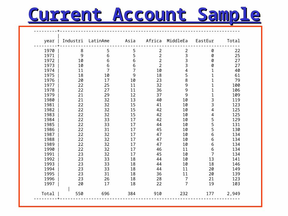
Current Account SampleCurrent Account Sample---------+--------------------------------------------------------------------- | year | Industri LatinAme Asia Africa MiddleEa EastEur Total---------+--------------------------------------------------------------------- 1970 | 8 5 5 2 2 0 22 1971 | 9 6 5 2 3 0 25 1972 | 10 6 6 2 3 0 27 1973 | 10 6 6 2 3 0 27 1974 | 11 7 7 10 4 1 40 1975 | 18 10 9 18 5 1 61 1976 | 20 17 10 23 8 1 79 1977 | 22 25 11 32 9 1 100 1978 | 22 27 11 36 9 1 106 1979 | 21 29 12 37 9 1 109 1980 | 21 32 13 40 10 3 119 1981 | 22 32 15 41 10 3 123 1982 | 22 32 15 42 10 4 125 1983 | 22 32 15 42 10 4 125 1984 | 22 33 17 42 10 5 129 1985 | 22 33 17 44 10 5 131 1986 | 22 31 17 45 10 5 130 1987 | 22 32 17 47 10 6 134 1988 | 22 32 17 47 10 6 134 1989 | 22 32 17 47 10 6 134 1990 | 22 32 17 46 11 6 134 1991 | 23 32 17 45 10 7 134 1992 | 23 33 18 44 10 13 141 1993 | 23 33 18 44 10 18 146 1994 | 23 33 18 44 11 20 149 1995 | 23 31 18 36 11 20 139 1996 | 23 26 18 28 7 21 123 1997 | 20 17 18 22 7 19 103 | Total | 550 696 384 910 232 177 2,949---------+---------------------------------------------------------------------

Median CA deficitsMedian CA deficits---------+--------------------------------------------------------------------- | year | Industri LatinAme Asia Africa MiddleEa EastEur Total---------+--------------------------------------------------------------------- 1970 | -0.41 4.06 0.94 0.92 7.86 0.86 1971 | -0.51 4.83 1.10 5.25 5.74 1.08 1972 | -1.06 1.70 1.57 6.16 2.88 0.44 1973 | 0.18 1.24 0.77 7.18 5.42 0.95 1974 | 2.94 4.10 3.02 2.39 0.14 1.50 2.97 1975 | 1.34 4.52 3.23 6.56 -2.73 3.52 3.40 1976 | 2.71 1.41 0.62 5.00 -6.65 3.81 3.27 1977 | 2.11 3.80 -0.03 4.24 -3.71 5.15 2.84 1978 | 0.68 3.48 2.74 9.95 3.01 1.88 3.60 1979 | 0.66 4.68 3.73 6.52 -8.89 1.54 3.32 1980 | 2.35 5.59 5.03 8.36 -3.96 4.95 4.66 1981 | 2.73 9.06 5.92 10.09 1.46 2.72 6.58 1982 | 2.02 7.60 5.10 9.85 -1.53 1.88 6.41 1983 | 0.88 4.70 7.18 6.59 5.10 1.48 4.33 1984 | 0.22 3.66 2.12 3.76 4.89 1.43 2.51 1985 | 0.98 2.07 3.13 4.42 2.61 1.51 2.91 1986 | -0.12 2.99 2.42 3.76 2.30 1.93 2.68 1987 | 0.42 4.15 1.34 5.22 3.04 0.76 2.61 1988 | 1.15 2.25 2.68 5.50 2.00 0.72 2.66 1989 | 1.54 4.41 3.35 3.76 -0.39 1.70 2.85 1990 | 1.60 3.00 3.41 3.78 -0.58 3.69 2.83 1991 | 0.91 4.83 3.17 3.64 9.74 0.70 3.02 1992 | 0.86 4.34 1.94 5.65 7.29 0.40 3.01 1993 | 0.55 4.60 4.18 6.81 4.20 1.58 3.18 1994 | -0.37 3.19 4.63 5.65 -0.38 1.39 2.49 1995 | -0.71 3.90 4.91 4.81 -2.14 1.99 2.70 1996 | -0.56 3.97 4.76 4.15 -0.99 4.50 3.28 1997 | -0.57 4.12 3.61 3.71 -2.39 6.29 2.94| Total | 0.77 4.12 3.14 5.33 1.95 1.93 3.17

Third quartile of CA deficitsThird quartile of CA deficits---------+--------------------------------------------------------------------- | group1 year | Industri LatinAme Asia Africa MiddleEa EastEur Total---------+--------------------------------------------------------------------- 1970 | 0.64 6.86 1.28 1.93 9.85 4.06 1971 | 0.43 7.77 1.74 8.28 9.31 4.55 1972 | 0.30 2.37 3.63 11.96 5.30 2.59 1973 | 1.33 4.12 1.30 9.99 5.81 4.12 1974 | 4.41 10.05 5.61 4.64 14.44 1.50 5.52 1975 | 4.46 6.78 5.06 8.44 13.98 3.52 7.75 1976 | 4.38 4.23 6.19 8.80 4.36 3.81 5.47 1977 | 3.62 7.37 4.49 7.86 2.47 5.15 6.35 1978 | 2.50 7.07 4.80 12.85 9.17 1.88 9.17 1979 | 2.76 6.60 6.57 12.30 5.17 1.54 7.62 1980 | 3.70 12.92 8.46 13.11 2.63 5.99 10.60 1981 | 4.32 15.06 10.04 12.85 5.85 7.38 11.76 1982 | 4.05 11.74 11.49 14.48 8.26 2.63 10.57 1983 | 2.41 8.33 9.01 12.39 7.73 2.61 8.33 1984 | 3.08 6.56 4.88 8.78 8.17 1.46 5.69 1985 | 3.75 6.05 4.82 9.68 7.45 1.85 6.42 1986 | 3.51 7.75 5.16 8.19 9.36 4.69 6.44 1987 | 3.24 8.79 4.07 9.69 6.35 2.53 6.35 1988 | 3.03 7.67 4.30 9.49 4.65 1.75 6.51 1989 | 3.60 7.61 5.91 7.02 5.43 2.02 5.69 1990 | 3.37 7.64 6.08 8.93 2.77 8.25 6.13 1991 | 2.78 11.57 6.61 9.05 17.96 3.51 7.57 1992 | 2.67 8.04 4.70 9.01 15.72 3.68 6.86 1993 | 1.65 8.81 6.42 8.80 11.45 4.45 7.86 1994 | 1.83 7.27 6.46 8.88 6.62 3.57 6.50 1995 | 1.64 5.42 8.06 10.42 4.24 5.54 6.61 1996 | 1.83 7.02 8.10 9.25 3.32 9.16 7.60 1997 | 1.91 5.93 6.89 7.05 2.94 11.07 6.29 1998 | | Total | 3.06 8.16 6.37 10.09 7.14 4.84 7.22---------+---------------------------------------------------------------------

Sudden Stops and CA Reversals ISudden Stops and CA Reversals I

B. Latin America

| Freq. Percent Cum.------------+----------------------------------- 0 | 359 81.04 81.04 1 | 84 18.96 100.00------------+----------------------------------- Total | 443 100.00

C. Asia

| Freq. Percent Cum.------------+----------------------------------- 0 | 250 85.91 85.91 1 | 41 14.09 100.00------------+----------------------------------- Total | 291 100.00

Sudden Stops and CA Reversals IISudden Stops and CA Reversals II

D. Africa

| Freq. Percent Cum.------------+----------------------------------- 0 | 230 72.56 72.56 1 | 87 27.44 100.00------------+----------------------------------- Total | 317 100.00

All Countries

| Freq. Percent Cum.------------+----------------------------------- 0 | 1580 83.29 83.29 1 | 317 16.71 100.00------------+----------------------------------- Total | 1897 100.00

Reversals and InvestmentReversals and Investmenta. Arellano-Bond Instrumental Variables

Arellano-Bond dynamic panel data Number of obs = 1800Group variable (i): imfcode Number of groups = 127

Wald chi2(5) = 181.56

Time variable (t): year min number of obs = 1 max number of obs = 25 mean number of obs = 14.17323------------------------------------------------------------------------------ | Robustinvgdp | Coef. Std. Err. z P>|z| [95% Conf. Interval]-------------+----------------------------------------------------------------invgdp | LD | .6212481 .0835012 7.44 0.000 .4575887 .7849075govcon | D1 | .0819257 .1063111 0.77 0.441 -.1264401 .2902916rev | D1 | -2.021207 .2545002 -7.94 0.000 -2.520018 -1.522396revlag | D1 | -.8834781 .2235849 -3.95 0.000 -1.321696 -.4452596trade | D1 | .0436178 .0127593 3.42 0.001 .0186101 .0686255_cons | -.0480371 .0169209 -2.84 0.005 -.0812014 -.0148727------------------------------------------------------------------------------Arellano-Bond test that average autocovariance in residuals of order 1 is 0: H0: no autocorrelation z = -4.46 Pr > z = 0.0000Arellano-Bond test that average autocovariance in residuals of order 2 is 0: H0: no autocorrelation z = -1.08 Pr > z = 0.2809

Reversals and GDP GrowthReversals and GDP GrowthCross-sectional time-series FGLS regression

Coefficients: generalized least squaresPanels: heteroskedasticCorrelation: no autocorrelation

Estimated covariances = 111 Number of obs = 1856Estimated autocorrelations = 0 Number of groups = 111Estimated coefficients = 32 Obs per group: min = 1 avg = 19.28987 max = 26 Wald chi2(31) = 708.80Log likelihood = -4913.651 Prob > chi2 = 0.0000

------------------------------------------------------------------------------ gdpgrowt | Coef. Std. Err. z P>|z| [95% Conf. Interval]-------------+---------------------------------------------------------------- invgdp | .1732786 .0129535 13.38 0.000 .1478901 .198667 govcon | -.044147 .0129061 -3.42 0.001 -.0694425 -.0188514 trade | .0066118 .0021185 3.12 0.002 .0024595 .010764 loggpp0 | -.7458834 .0754805 -9.88 0.000 -.8938225 -.5979443 rev | -.8387433 .2063497 -4.06 0.000 -1.243181 -.4343053 revlag | -.3106008 .2014468 -1.54 0.123 -.7054293 .0842277

_cons | 7.826786 .8179467 9.57 0.000 6.22364 9.429932------------------------------------------------------------------------------

5. The Current Account and 5. The Current Account and Currency Crises: How Strong is Currency Crises: How Strong is

the Link?the Link?

Frequency of CrisesFrequency of CrisesA: aevent

(mean) | event | Freq. Percent Cum.------------+----------------------------------- 0 | 2818 94.09 94.09 1 | 177 5.91 100.00------------+----------------------------------- Total | 2995 100.00

B. aevent2

aevent2 | Freq. Percent Cum.------------+----------------------------------- 0 | 2318 95.79 95.79 1 | 102 4.21 100.00------------+----------------------------------- Total | 2420 100.00

C. acrisis

(mean) | crisis | Freq. Percent Cum.------------+----------------------------------- 0 | 2548 90.26 90.26 1 | 275 9.74 100.00------------+----------------------------------- Total | 2823 100.00

D. acrisis2

acrisis2 | Freq. Percent Cum.------------+----------------------------------- 0 | 1564 88.91 88.91 1 | 195 11.09 100.00------------+----------------------------------- Total | 1759 100.00

Reversals and CrisesReversals and Crises

Case: Aevent definition of crisis;Exposed: Reversal1 definition of current account reversal

Proportion | Exposed Unexposed | Total Exposed-----------------+------------------------+---------------------- Cases | 28 124 | 152 0.1842 Controls | 410 1793 | 2203 0.1861-----------------+------------------------+---------------------- Total | 438 1917 | 2355 0.1860 | | | Point estimate | [95% Conf. Interval] |------------------------+---------------------- Odds ratio | .9874902 | .6481554 1.504718(Cornfield) Prev. frac. ex. | .0125098 | -.504718 .3518446(Cornfield) Prev. frac. pop | .0023282 | +----------------------------------------------- chi2(1) = 0.00 Pr>chi2 = 0.9536

Sustained Reversals and CrisesSustained Reversals and Crises

Case: Aevent definition of crisis;Exposed: Reversaln1 definition of current account reversal

Proportion | Exposed Unexposed | Total Exposed-----------------+------------------------+---------------------- Cases | 52 35 | 87 0.5977 Controls | 563 679 | 1242 0.4533-----------------+------------------------+---------------------- Total | 615 714 | 1329 0.4628 | | | Point estimate | [95% Conf. Interval] |------------------------+---------------------- Odds ratio | 1.791829 | 1.15408 2.781784(Cornfield) Attr. frac. ex. | .4419112 | .1335086 .6405185(Cornfield) Attr. frac. pop | .2641308 | +----------------------------------------------- chi2(1) = 6.82 Pr>chi2 = 0.0090

Probit Model of CrisesProbit Model of CrisesA. ACRISIS

Probit estimates Number of obs = 931 Wald chi2(17) = 56.70 Prob > chi2 = 0.0000Log likelihood = -274.9083 Pseudo R2 = 0.1103

------------------------------------------------------------------------------ | Robust acrisis | dF/dx Std. Err. z P>|z| x-bar [ 95% C.I. ]---------+-------------------------------------------------------------------- comrat | .0033323 .0017217 1.90 0.057 21.0027 -.000042 .006707 conrat | -.0010057 .0007642 -1.30 0.193 32.5979 -.002504 .000492 varrat | -.0025776 .0016872 -1.51 0.131 21.9735 -.005884 .000729fdistock | -.0052372 .0022728 -2.27 0.023 2.62669 -.009692 -.000783shorttot | .0019636 .0015704 1.27 0.203 14.6745 -.001114 .005041 pubrat | .0009573 .0010942 0.88 0.381 72.419 -.001187 .003102multirat | .0020735 .0008301 2.44 0.015 21.4711 .000447 .0037 debty | .0002462 .0002104 1.16 0.247 59.5954 -.000166 .000659reservem | -.0000357 .0000375 -0.94 0.345 324.331 -.000109 .000038 defrat | .0011096 .0016363 0.68 0.497 5.15325 -.002097 .004317 dlcred | .0010474 .0003367 3.23 0.001 21.875 .000387 .001707 dly | -.0027143 .0013687 -2.00 0.046 3.51322 -.005397 -.000032 istar | .0020625 .0030204 0.68 0.497 8.64066 -.003857 .007982overvaln | .0001934 .0004058 0.48 0.634 -7.88634 -.000602 .000989 trade | -.0009073 .0005028 -1.74 0.082 46.3937 -.001893 .000078 govcon | -.0001539 .0017092 -0.09 0.928 14.0511 -.003504 .003196 cad | .0031167 .0016689 1.83 0.067 4.36866 -.000154 .006388---------+-------------------------------------------------------------------- obs. P | .1031149 pred. P | .0773022 (at x-bar)------------------------------------------------------------------------------ z and P>|z| are the test of the underlying coefficient being 0

Probit Model of Crises IIProbit Model of Crises IIProbit estimates Number of obs = 934 Wald chi2(17) = 70.66 Prob > chi2 = 0.0000Log likelihood = -189.0942 Pseudo R2 = 0.2072

------------------------------------------------------------------------------ | Robust aevent | dF/dx Std. Err. z P>|z| x-bar [ 95% C.I. ]---------+-------------------------------------------------------------------- comrat | .0003686 .0008709 0.42 0.671 20.962 -.001338 .002075 conrat | -.000823 .0004234 -1.82 0.069 32.6715 -.001653 6.9e-06 varrat | -.0007301 .0008421 -0.86 0.388 21.9302 -.002381 .000921fdistock | -.0033417 .0012196 -2.69 0.007 2.62084 -.005732 -.000951shorttot | -.0000499 .0008731 -0.06 0.955 14.6571 -.001761 .001661 pubrat | -.0001298 .0006229 -0.21 0.836 72.4703 -.001351 .001091multirat | -.0002948 .0005312 -0.56 0.578 21.4961 -.001336 .000746 debty | .0002863 .0001209 2.49 0.013 59.7336 .000049 .000523reservem | -.0000194 .0000197 -1.01 0.315 325.061 -.000058 .000019 defrat | .0016828 .0009088 1.85 0.065 5.21531 -.000098 .003464 dlcred | .0004188 .0002005 2.53 0.012 21.8889 .000026 .000812 dly | -.001096 .0008227 -1.34 0.179 3.51907 -.002708 .000516 istar | -.0000236 .0017433 -0.01 0.989 8.63804 -.00344 .003393overvaln | -.0003881 .0002363 -1.64 0.102 -7.82043 -.000851 .000075 trade | -.001114 .0003071 -3.06 0.002 46.3682 -.001716 -.000512 govcon | -.0037107 .0012011 -2.97 0.003 14.071 -.006065 -.001357 cad | .0003098 .0010221 0.30 0.764 4.37692 -.001693 .002313---------+-------------------------------------------------------------------- obs. P | .0706638 pred. P | .0296255 (at x-bar)------------------------------------------------------------------------------ z and P>|z| are the test of the underlying coefficient being 0

Crises Excluding Africa ICrises Excluding Africa IProbit estimates Number of obs = 586 Wald chi2(17) = 47.59 Prob > chi2 = 0.0001Log likelihood = -172.36345 Pseudo R2 = 0.1381

------------------------------------------------------------------------------ | Robust acrisis | dF/dx Std. Err. z P>|z| x-bar [ 95% C.I. ]---------+-------------------------------------------------------------------- comrat | .0029271 .0020359 1.42 0.157 26.3123 -.001063 .006917 conrat | -.0012155 .0008973 -1.32 0.186 28.4099 -.002974 .000543 varrat | -.0020405 .0019753 -1.02 0.306 27.1534 -.005912 .001831fdistock | -.005784 .0024845 -2.24 0.025 3.17666 -.010653 -.000915shorttot | .0016729 .002148 0.81 0.418 15.9367 -.002537 .005883 pubrat | .0014678 .0013265 1.13 0.258 69.9099 -.001132 .004068multirat | .0026282 .000894 2.77 0.006 19.8038 .000876 .00438 debty | 3.91e-06 .0003489 0.01 0.991 53.1143 -.00068 .000688reservem | -7.38e-06 .0000403 -0.18 0.855 412.658 -.000086 .000072 defrat | .0010166 .0019793 0.52 0.606 4.5621 -.002863 .004896 dlcred | .0008556 .0003243 2.85 0.004 25.8435 .00022 .001491 dly | -.0021348 .0017565 -1.24 0.215 3.8471 -.005577 .001308 istar | .0026776 .0036062 0.73 0.466 8.48895 -.00439 .009746overvaln | -.0000309 .0005285 -0.06 0.953 -5.23607 -.001067 .001005 trade | -.0010877 .0006823 -1.48 0.140 47.171 -.002425 .00025 govcon | .0017909 .0023691 0.76 0.448 13.3222 -.002852 .006434 cad | .0048408 .0021958 2.08 0.037 3.62618 .000537 .009145---------+-------------------------------------------------------------------- obs. P | .1075085 pred. P | .0718758 (at x-bar)------------------------------------------------------------------------------ z and P>|z| are the test of the underlying coefficient being 0

Crises Excluding Africa IICrises Excluding Africa IIProbit estimates Number of obs = 588 Wald chi2(17) = 64.52 Prob > chi2 = 0.0000Log likelihood = -121.01338 Pseudo R2 = 0.2262

------------------------------------------------------------------------------ | Robust aevent | dF/dx Std. Err. z P>|z| x-bar [ 95% C.I. ]---------+-------------------------------------------------------------------- comrat | .0005594 .0009588 0.58 0.561 26.2654 -.00132 .002439 conrat | -.0004993 .0005171 -0.89 0.373 28.4811 -.001513 .000514 varrat | -.0002586 .000949 -0.27 0.787 27.1044 -.002119 .001601fdistock | -.0029753 .0012766 -2.27 0.023 3.16641 -.005477 -.000473shorttot | .0009613 .0011325 0.91 0.363 15.9162 -.001258 .003181 pubrat | .0012306 .0008209 1.71 0.086 69.9671 -.000378 .00284multirat | -.0006806 .0006162 -1.21 0.227 19.7912 -.001888 .000527 debty | .0000792 .0001567 0.51 0.613 53.3316 -.000228 .000386reservem | -.0000334 .0000222 -1.57 0.115 412.677 -.000077 .00001 defrat | .0011607 .0009477 1.19 0.233 4.61603 -.000697 .003018 dlcred | .0002325 .0001554 1.85 0.064 25.8675 -.000072 .000537 dly | -.0015439 .0009927 -1.73 0.084 3.85051 -.003489 .000402 istar | .0001112 .0019632 0.06 0.955 8.4883 -.003737 .003959overvaln | -.0003815 .0002373 -1.49 0.137 -5.18871 -.000847 .000084 trade | -.0010118 .0003537 -2.52 0.012 47.1363 -.001705 -.000318 govcon | -.0021182 .0012636 -1.57 0.116 13.35 -.004595 .000358 cad | .0018845 .0011319 1.62 0.105 3.64741 -.000334 .004103---------+-------------------------------------------------------------------- obs. P | .0748299 pred. P | .0253162 (at x-bar)------------------------------------------------------------------------------ z and P>|z| are the test of the underlying coefficient being 0

Crises Excluding Africa IIICrises Excluding Africa IIIEXCLUDES RESERVES AND DEBTProbit estimates Number of obs = 591 Wald chi2(15) = 65.13 Prob > chi2 = 0.0000Log likelihood = -124.15434 Pseudo R2 = 0.2198

------------------------------------------------------------------------------ | Robust aevent | dF/dx Std. Err. z P>|z| x-bar [ 95% C.I. ]---------+-------------------------------------------------------------------- comrat | -.0000411 .0008099 -0.05 0.960 26.3022 -.001629 .001546 conrat | -.0005226 .000528 -0.93 0.354 28.4596 -.001557 .000512 varrat | .000294 .000864 0.34 0.731 27.1331 -.001399 .001988fdistock | -.0034274 .0013471 -2.52 0.012 3.15382 -.006068 -.000787shorttot | .0009178 .0011867 0.81 0.417 15.9153 -.001408 .003244 pubrat | .0012746 .0008641 1.65 0.099 70.0393 -.000419 .002968multirat | -.0007383 .0006296 -1.27 0.202 19.7436 -.001972 .000496 defrat | .0017021 .000881 1.85 0.064 4.68826 -.000025 .003429 dlcred | .0002103 .0001511 1.66 0.096 26.0009 -.000086 .000506 dly | -.0018491 .0010946 -1.87 0.062 3.83729 -.003995 .000296 istar | .0003013 .0020829 0.14 0.885 8.48095 -.003781 .004384overvaln | -.000391 .0002352 -1.52 0.128 -5.48445 -.000852 .00007 trade | -.0010849 .0003564 -2.56 0.011 47.1491 -.001783 -.000386 govcon | -.0019375 .0012981 -1.43 0.153 13.455 -.004482 .000607 cad | .0024955 .001186 2.09 0.037 3.71074 .000171 .00482---------+-------------------------------------------------------------------- obs. P | .0761421 pred. P | .0279486 (at x-bar)------------------------------------------------------------------------------ z and P>|z| are the test of the underlying coefficient being 0

6. Concluding Remarks: Does 6. Concluding Remarks: Does the Current Account Matter?the Current Account Matter?

If this question is interpreted broadly, as meaning that there are costs involved in running “very large” deficits, the answer is a “yes.”“yes.”– Current account reversals are quite common and,

even if they do not always lead to crises, they are costly.

– Moreover, the evidence presented here suggests that, for some regions, a higher CA deficit will increase the probability of a currency crisis.