N.W. Posthumus Institute of Economic and Social History, Groningen

and

Hitotsubashi University 21st Century Program, Research Unit for Statistical Analysis in Social

Sciences, the Institute of Economic Research, Hitotsubashi University

Technology and Long-run Economic Growth in Asia

Capital Formation and Economic Growth in Indonesia,

1951-2004

Pierre van der Eng

September 9th, 2005 Sano-Shoin, Hitotsubashi University,

Kunitachi, Tokyo

Capital Formation and Economic Growth in Indonesia, 1951-2004

Pierre van der Eng

School of Business and Information Management Faculty of Economics and Commerce

The Australian National University Canberra ACT 0200

Australia Fax: +61 2 6125 5005

E-mail: pierre.vandereng@anu.edu.au

Abbreviated title: Capital Formation and Economic Growth Abstract This paper makes long-term estimates of gross fixed capital formation that are disaggregated by categories of productive assets. These data, combined with a choice of the probable average asset lives and a feasible asset retirement method are used in a Perpetual Inventory Method to make disaggregated estimated of gross fixed capital stock in Indonesia. The estimates indicate that Indonesia’s capital stock increased substantially during the 1990s until 1998-99, largely in the category non-residential structures. The capital-output ratios for that decade suggest significant overinvestment and underutilisation of capital stock in the late-1990s. Keywords: JEL-codes: This (unfinished) version: 3 September 2005. This is work in progress. Please do not quote.

1

Capital Formation and Economic Growth in Indonesia, 1951-2004

1. Introduction What is the stock of capital goods in Indonesia and to what extent has it contributed to the generation of production and income? To what extent is the Indonesian economy currently operating below capacity? These questions were long difficult to answer because of the lack of good estimates of capital stock. In recent years, the Indonesian Bureau of Statistics (Badan Pusat Statistik, BPS) and Bank Indonesia (BI) made estimates of capital stock. However, the focus of this work was the estimation of capital stock in recent years in order to gauge the degree to which the Indonesian economy suffered from productive overcapacity since the 1997-98 crisis in the light of low rates of economic growth following decades rates of high investment. The estimates were not made with times series analysis of productivity change and the contribution of capital to long-term economic growth in Indonesia in mind. This paper explains the methodology used to estimate Indonesia’s capital stock over more than 50 years. These estimates will be used to eventually gauge changes in Total Factor Productivity in Indonesia. The estimation and the analysis are necessarily tentative, due to the assumptions that had to be made in the estimation process and the fact that the underlying data are not necessarily as accurate as possible. It is hoped that the estimates can be improved as better underlying data become available, and that the estimates can be extended further back in time. 2. Relevance of the estimates: Capital formation in economic growth A low rate of capital formation, caused by a lack of savings or restricted access to foreign sources for investment, has been identified as one of the major impediments to economic development. Especially in the 1950s, low savings rates and low rates of capital formation were widely regarded as the prime bottleneck in development (Abbas 1955). Economic historians, such as W.W. Rostow, suggested that a sudden increase of the Capital-Output Ratio (COR) marked an initial phase in economic development, which in the past had lifted now-developed economies out of stagnation and into a phase of self-sustaining economic growth during which the COR increased further. Later studies indicated that there is little evidence for now-developed countries that the COR has moved in any specific direction over time (Kuznets 1963; Ohkawa 1984; Le Thanh 1988). Kuznets (1964: 41) maintained that the contribution of the increases in the stock of labour (unweighted by skill and education) and capital (reproducible and non-reproducible) to the increase of per capita income over long periods in the major developed countries ranged only between 15-20%, and concluded: ‘By far the major proportion in the course of modern economic growth must be attributed to changes in skill, education, and so on, of the labour force, or to other sources of the large increase in productivity per man-hour combined with the unit of material capital - and not to any

2

increase in inputs per head.’ Other authors, including Kendrick (1993), noted that more important than capital formation were improved efficiency in the use of

resources and the movement of resources from less productive to more productive sectors. Although the contribution of capital formation to overall economic growth may be more limited than initially thought, there are good reasons to gauge it. Particularly the process of technical change in manufacturing tends to be characterised by an increasing use of capital goods in the production process, because they allow a higher output per worker. Maddison (1991: 41) pointed out that, although the COR may not increase dramatically, economies do devote an increasing proportion of GDP to investment in capital goods during the process of economic development. Fast growing economies generally do spend more on capital formation than countries with low growth rates of output. Hence, a higher rate of capital formation is perhaps not a precondition for economic development, but rather concomitant to that process. The role of capital formation in early phases of development should not be overestimated. It is easy to see that in the early phases of development immediate changes in the major economic sectors of developing countries do not require large-scale capital formation, e.g. in agriculture trade, crafts and small industries. As far as historical evidence goes, much of public infrastructure (roads, railways, etc.) was developed in the course of economic development, not prior to it. Still, no attempt to account for growth is complete without estimates of total factor productivity and factor income, for which estimates of capital stock are required. [Include brief discussion of contribution of capital formation to GDP(E) growth. For this exercise no estimates of capital stock are required. Also note ICOR estimates.] 3. Previous work involving Indonesia The role of capital formation and the measurement of capital formation in Southeast Asia received considerable attention in the 1950s and 1960s. Debate has indicated that the available statistical evidence on low rates of saving and capital formation was very weak, due to underdeveloped national accounting procedures. It was also pointed out that published rates of capital formation often ignored capital formation in agriculture and small-scale industries.1 In this respect the inclusion and valuation of farm structures is crucial, because of the relative size of the agricultural sector and the fact that structures generally have a much higher capital-output ratio than equipment and machinery. Interest in gauging capital formation in Indonesia increased in the 1950s, largely as part of the process of macro-economic planning at the Biro Perancang Negara (BPN),

1. Abraham (1958, 1967), Oshima (1961), Hooley (1964) and Ramamurti and Pedersen (1965) discussed the statistical inaccuracies and differences in concepts used in the estimation of capital stock and gross capital formation in Asia.

3

which culminated in the first five-year plan (1956-60). Much of the early work at BPN focused on identifying ways to spur the rate of capital formation (see e.g. BPN 1957:

496-506). As national accounting was in its infancy, the first estimates of gross capital formation and depreciation were necessarily rough and incomplete.2 Little information is available about the methodology that was used at the time, but the BPN estimates for 1958-59 are significantly lower than estimates made at BPS for the same and later years, after BPS had been given responsibility for the compilation of national accounts in 1960.3

BPS has since published estimates of gross fixed capital formation (GFCF) in current and constant prices since 1960, which underwent several revisions (1960-73 1960 prices, 1971-83 1973 prices, 1983-93 1983 prices, 1988-2003 1993 prices, 2000-04 2000 prices). The revisions not only involved a change of the benchmark year for the constant prices series. They also involved upward revisions of estimates of GFCF, although it is unknown what exactly led to the revisions, as BPS never formally published its estimation procedures. Hence, apart from disclosures that BPS has always estimated GFCF on the basis of the commodity flow method, little is known about the details of calculation. As a consequence of the use of the commodity flow method, there is no distinction between GFCF in the public and private sectors.4 In addition, the difference between net and gross fixed capital formation has always been assumed at 5% fixed and flat rate of depreciation.5

The BPS estimates of capital formation in constant prices have been used to estimate capital stock. Sundrum (1986: 55, 68) used estimates of net capital formation to extrapolate a rough guess of total net capital stock in 1960 (obtained from India) to generate a net capital stock series for 1960-81 in 1973 prices. Keuning (1988, 1991) used Incremental Capital Value Added Ratios (ICVAR) for 1975-80 and sectoral data on value added (partially estimated), to estimate GFCF during 1953-85 and gross fixed capital stock (GFCS) during 1975-85 in 1980 prices for 22 economic sectors and three types of capital goods. Van der Eng (2002: 148-52, 174-75) extended Keuning’s 1975-85 estimates to create crude estimates of total gross fixed capital stock in 1983 prices for 1952-99. As part of their multi-country studies, Nehru and Dareshwar (1993), King and Levine (1994) and Young (1995) used data on GFCF in Indonesia reported by international agencies to cobble together estimates of capital stock in constant prices using a Perpetual Inventory Model (PIM) approach. However, they took no account of inconsistencies and underestimation in these GFCF data. Sigit (2004: 102-103, 124-125)

2. See e.g. estimates for 1951-52 Neumark (1954: 354-55) or 1951-55 (BPN 1957: 496-506; Muljatno 1960: 165-66, 189). The latter estimates are the same as the 1951-59 estimates (Joesoef 1973: p.32) made at Biro Keuangan dan Ekonomi (BKE) at the Sekretariat Negara, which suggests that BKE continued the work on Indonesia’ s national accounts after BPN was disbanded in August 1959. 3. For example, where BKE estimated GFCF in 1958 of 8.2 billion Rupiah, BPS estimated 19.8 billion Rupiah. 1958-59 from unpublished BPS (1969) data; 1960-68 from Sudirman (1972) and BPS (1970). 4. The only estimates of public capital formation are for 1981-99 (Everhart and Sumlinski 2003). They suggest an average share of 34% public investment. For 1951-59, BKE estimates suggest a 32% average share (Joesoef 1973: p.32). 5. Neumark (1954) also assumed 5%, but BPN/BKE assumed 3% in the 1950s (Muljatno 1960: 164).

4

used a similar approach but corrected the GFCF series for inconsistency and underestimation to estimate total GFCS in 1993 prices for 1975-2000.

Estimates of capital stock for manufacturing industry only were made by Hill et al. (1997) for 1976-91 and Timmer (1999) for 1975-95 on the basis of investment data from the annual statistics on industrial production, using a PIM approach. BPS and BI recently made the most elaborate estimates of capital stock. BPS estimated gross and net fixed capital stock in current and 1993 prices for 1980-94 (BPS 1997). Few details of the BPS methodology are publicly available, but it consisted of first disaggregating GFCF from the national accounts into the relevant categories of capital goods identified in the 1980, 1985 and 1990 Input-Output (I-O) Tables, and interpolations of these benchmark years (Sigit 2004: 101-102, 124). BI estimated gross and net fixed capital stock in 1993 prices for 1960-2002 (Wicaksono 2002; Wicaksono and Ariantoro 2003; Yudanto et al. 2005). BI used the same approach as BPS, but included the 2000 I-O Table. It interpolated the GFCF benchmark years from the I-O Tables and obtained a new time series of GFCF for 1980-2000. GFCF was then apportioned to categories of investment in capital goods and to economic sectors on the basis of the I-O tables to generate disaggregated GFCF data in constant prices. The constant price series were combined with assumptions of average asset life in different categories, and assumptions about the retirement of capital goods, in order to produce estimates of capital stock. As the longest time span of assets was assumed to be 20 years (for buildings), the first ‘complete’ estimate of capital stock was for 1999. That year was extrapolated on the basis of a ‘gross-up’ method, first for 1980-98 and then for 1960-79. Although a major step forward, the BI estimates contain several problems: 1. Underestimation of GFCF not accounted for. Saleh (1997: 4) noted that the BPS

estimates of GFCF are incomplete, as they only cover the acquisition of new capital goods that were domestically produced and new and used imported capital goods (all estimated on the basis of the commodity flow method). Estimates of GFCF therefore exclude investment in cultivated assets, particularly in agriculture, such as perennial crops and livestock.6 They also exclude new investment for the improvement of existing assets (such as roads and other existing infrastructure). Nor is the disposal of capital goods through exports (e.g. ships and aeroplanes) accounted for. Another problem is that the use of various materials in the construction industry, such as steel and electrical equipment, are not fully accounted for (Rachman 2004: 2, 4)

2. 1980 Starting point. This ignores information available from the 1971 and 1975 I-O Tables.

3. Methods. The ‘gross-up’ method and the methods used to allocate GFCF to types of capital goods and to economic sectors are not unambiguously explained and therefore

6. The coverage of livestock is incomplete in the I-O Tables and non-existent in the national accounts. Investment in perennials is not covered at all. A major prerequisite for the analysis of long-term economic growth in Indonesia would be the estimation of capital formation and capital stock in agriculture, given the prominence of the agricultural output in the economy until the 1970s. This could be done as outlined in Shukla (1965).

5

not replicable.

4. Assumptions about average asset life. These were obtained from BPS, which in turn appears to have obtained them from Decrees of the Minister of Finance of Indonesia (No.961/1983 and 826/1984 on taxation) containing allowable rates of depreciation for broad asset groups (BPS 1997: 3, 5).7 Unfortunately, tax office estimates of depreciation in other countries not always resemble true asset lives (see e.g. Lützel 1977: 69). Indonesia is not likely to be an exception. For example, the Indonesian taxation rules allow companies in capital-intensive industries to employ an accelerated depreciation relative to other countries (Gordon 1998: 25). Indeed the average asset lives used by BPS and BI are low compared to those of other countries (see e.g. Blades 1993). Consequently, BPS and BI may have underestimated capital stock.

5. Net fixed capital stock estimate. This is calculated with straight-line depreciation [presumably, actually not clear using the 5% BPS rate of depreciation] to account for the consumption of fixed capital, rather than the retirement of assets. If it is the BPS 5%, it should be noted that it is not on any knowledge of the true rate of depreciation.

4. Estimating Capital Formation and Capital Stock The estimation presented here consists of two stages: 1. re-estimation of GFCF in 1983 prices for 1951-2004, apportioned to 28 types of capital

goods; 2. the use of assumptions about asset lives and a simple PIM to aggregate the GFCF

data. 4.1 Re-estimating GFCF, 1951-2004 The following steps were taken to re-estimate GFCF: a. Creation of a (single) GFCF price index by linking the implicit deflators of GFCF from the

national accounts to form a new index with 1983 =100 for 1951-2004. b. Interpolation of total GFCF from the I-O benchmark years with growth rates of GFCF

in current prices from the national accounts to yield a new time series of total GFCF

7. The Indonesian government simplified its tax system in 1984 (with further changes in 1995 and 2000) with Law No.7/1983, which gave depreciation rates for buildings and 4 asset groups by useful life. Further regulations interpreted these rules (e.g. 961/1983 = No. 961/KMK.04/1983). The latest regulation, Keputusan Menteri Keuangan (Decree of the Minister of Finance) No. 138/KMK.03/2002, specified a range of specific assets in each of these 4 groups. The Indonesian accounting standards (particularly Pernyataan Standar Akuntansi Keuangan (PSAK) No.17 Akuntansi Penyusutan and No.46 Standar Akuntansi Pajak Penghasilan), issued by the Indonesian Institute of Accountants, propose different rates that are broadly in line with the depreciation rates for income tax purposes. The standards have no legal backing, so that companies are not obliged to follow them. Still, a cursory check of the financial statements of some major public companies in Indonesia suggests that they largely follow the tax and PSAK rates. The Indonesian public service accounting standard (Standar Akuntansi Pemerintahan Peryataan, particularly No.07 Tentang Akuntansi Aset Tetap) does not propose depreciation rates for specific types of assets.

6

1971-2000 in current prices. c. Deflation of total GFCF with the GFCF price index from a. to form a new time

series of total GFCF 1971-2000 in 1983 prices. d. Extrapolation of GFCF in constant prices for 1951-70 and 2000-04 with growth rates

of GFCF in constant prices from the national accounts and Joesoef (1973) to form a new series of GFCF in constant 1983 prices.

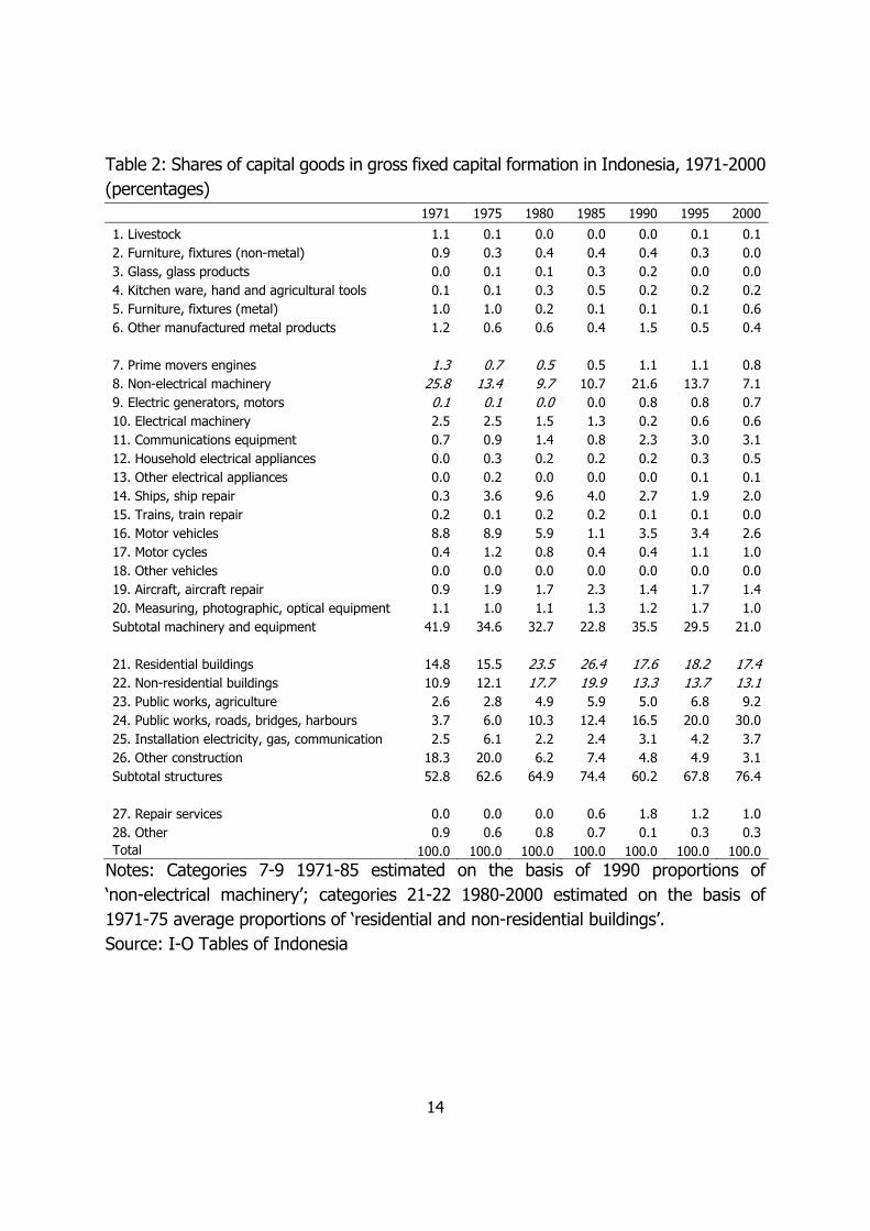
e. GFCF was apportioned to different categories of capital goods by using the interpolated shares shown in Table 2 for the I-O benchmark years and GFCF from d. Table 2 shows that most GFCF was in the form of structures. Its share increased from 53% in 1971 to 76% in 2000. To the detriment of the share of machinery and equipment which decreased from 41% to 21%.

f. Extrapolation of the total of categories 7-20 and 21-26 1958-70 on the basis of GFCF in 1960 prices in ‘construction and works’ and ‘machinery and equipment’ from BPS (1969), Tjahjani (1972), BPS (1970), Donges et al. (1973: 212). Deduction of these two groups from the GFCF series from d. to form the category 1958-70. Allocation of the results to categories in these groups, using 1971 shares.

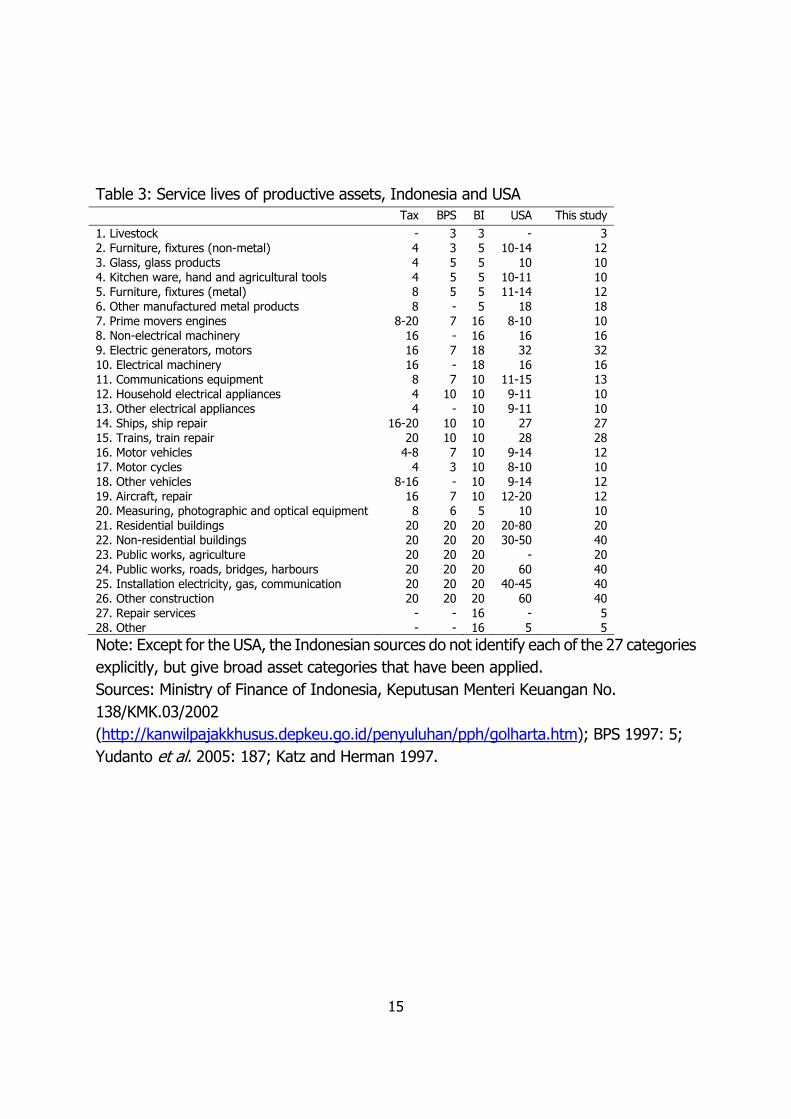
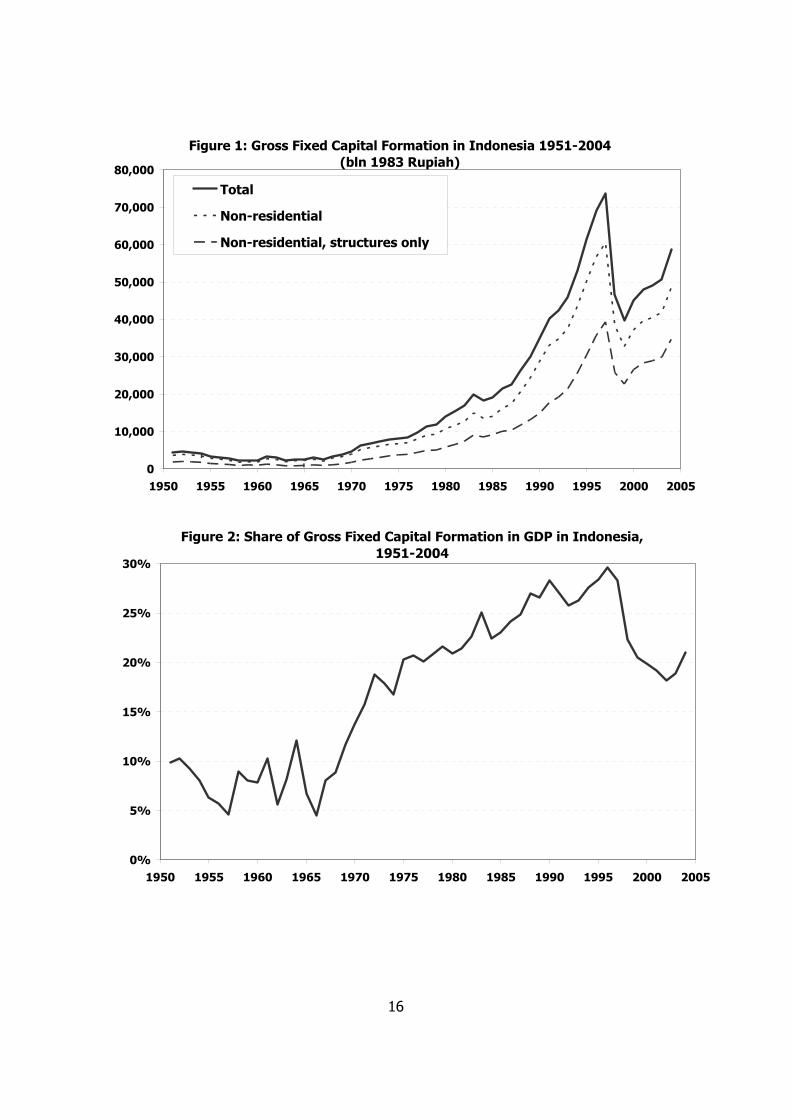
g. Extrapolation of 1951-57 CFCF from d. by using 1958 category shares. h. Extrapolation of 2001-04 by multiplying 2000 category shares and GFCF from d. The results are included in Appendix Table A.1 and are summarised in Figure 1, which shows that GFCF quadrupled from the mid-1960s to the mid-1980s, and then quadrupled again to the mid-1990s. The 1997-98 crisis and its aftermath caused a significant fall in GFCF, although the trough in 1999 was still at a level comparable to 1991. The chart also indicates that the trend was largely driven by non-residential capital stock, particularly non-residential buildings. Figure 2 shows a similar pattern, with GFCF increasing from a level of 7.5% until the mid-1960s to 24% in the 1980s and a significant 27% in the 1990s until the 1997-98 crisis. 4.2 Estimating GFCS, 1950-2004 The estimates of GFCF in Appendix Table A.1 are used to estimate GFCS. For this purpose, we need indications of the average working life of different categories of capital goods. Table 4 summarises the available information on average asset lives in Indonesia. As noted in section 3, this information is largely based on taxation data. To indicate that the estimates may be rather low, estimates of the service life of assets used in the calculation of capital stock in the USA are included in Table 4. Particularly the 20 years assumed in Indonesia for constructions appears to be very low. As far as available, estimates of asset lives differ considerably across countries (Blades 1993). Such differences seriously impair inter-country comparisons and, for instance, led Maddison (1995) to re-estimate capital stock in several countries using USA-based standardised asset lives of 39 years for ‘non-residential structures’ and 14 years for ‘machinery and equipment’. Also to facilitate international comparison, this study uses average asset lives that are generally higher than in the BPS-BI studies, and more

7

resembling the asset lives in the USA. It is possible to assume that the average working life of particular categories

of productive assets in Indonesia changed over time. For example, casual impressions may suggest that public structures such as railway stations and irrigation structures built in the past may have lasted longer than those built in later decades, which also crucially depend on whether regular maintenance work was carried out. However, there is no way to generalise such impressions. Another issue to consider is the method of asset retirement. Unfortunately, little with general validity is known about the retirement of capital goods by companies in Indonesia. Comparisons of the different methods indicated that GFCS estimates are relatively insensitive to the retirement pattern used (Blades 1983: 27; O’Mahony 1996; Yudanto et al. 2005: 18687). For the sake of simplicity, we use straight line retirement until the end of the average asset life. We did not estimate net fixed capital stock. It is a useful concept for surveying a country’s national wealth and certainly appropriate for company accounting purposes where depreciation records the loss of the value of assets used for production purposes to approximate the ‘fair value’ of assets. However, when depreciation is faster (for instance for taxation reasons) than the actual efficiency decline of capital goods, the net fixed capital concept is likely to understate the capital stock employed for production purposes. In addition, there is no conclusive evidence of the rate of consumption of fixed capital in Indonesia and/or the rate of efficiency decline of capital goods. Hence, we opted not to estimate net fixed capital stock. The disaggregated annual estimates of GFCF, average asset life and the method of depreciation allow the estimation of GFCS on the basis of the PIM, as recommended in the 1993 UN System of National Accounts. The results are contained in Appendix Table A.2 and are summarised in Figure 3. As the longest lifespan of our asset categories is 40 years, the first ‘complete’ estimates of GFCS are for 1990. During 1990-97 GFCS doubled before the rate of growth slowed following the 1997-98 crisis. The chart also indicates that the trend was largely driven by non-residential capital stock, particularly non-residential buildings, as already suggested by Figure 1. Figure 4 confirms these impressions. Since the early 1970s, growth of total GFCS has been 10-12% per year on average, broadly in line with the trend in the category non-residential structures, rather than machinery and equipment. Figure 5 shows the shares of the main categories of GFCS. It indicates that the share of non-residential structures increased significantly since the early 1990s. This was in part a consequence of the growth of this category in GFCF. Figure 6 shows different available estimates of the COR. For productive purposes, the ratio based on total non-residential GFCS is most significant. It clearly shows that after stagnation until the early 1980s, the ratio started a gradual increase until 1997, when the fall of GDP caused this COR to jump from 2.0 in 1997 to 2.5 in 1999. The gradual increase since the early-1980s can be interpreted as a consequence of accelerated structural change away from agriculture towards greater economic dependence on production, income and employment in industry. The share of agriculture, with its relatively low COR,

8

in total GDP in current prices decreased continuously from an average of 54% in 1958-60 to 18% in 1996-97. In addition, the share of industrial production from a

lowly 8-9% during both the 1960s and 1970s to 38% in 1996-97, suggests that the increase in the COR could have been largely triggered by investment in manufacturing industry. On the other hand, accelerated investment in non-residential constructions to 12% per year during 1991-97 may indicate overinvestment in sectors that are able to rapidly absorb such investment, particularly retail, real estate business services, hotels.8

Figure 7 compares the estimates of COR in this study with the COR estimates from other studies. It is clear that all trends are of similar proportions to our estimates, ignoring the low levels in the BPS estimates for 1980-91, which is due to the ‘build up’ of aggregated GFCF from the first ‘instalment’ in 1980. The BI estimates are significantly lower than ours, which is largely due to the shorter asset lives used in the BI study (see Table 4), particularly for constructions. How plausible are these different COR level estimates? One way to check that is through comparison with COR estimates of other countries. For Southeast Asia, Snodgrass (1966: 68, 75) assumed CORs for Malaya of 1.4-1.7 in 1954 and 1.8-1.9 in 1963. Chou (1966: 73) suggested a COR of 2 for Malaya in the early 1950s. Historical COR estimates have been presented for Japan and India. Based on an estimated capital stock excluding residential buildings, the COR in Japan increased from 1.81 in 1890 to 1.96 in 1910, 2.59 in 1930 and 2.17 in 1960 (Minami 1986: 190). Goldsmith (1985) presented historical balance sheets of national wealth for 20 countries, including Japan and India. The definition of wealth includes land, structures, precious metals and financial assets. With capital defined as net reproducible tangible assets, India’s COR increased from 1.43 in 1850 to 1.61 in 1913, 2.24 in 1950 and 3.92 in 1978, while Japan's COR increased from 3.38 in 1875 to 3.75 in 1913, and decreased to 2.71 in 1939, 1.39 in 1950 and 2.27 in 1987 (Goldsmith 1985: 40). Defined more narrowly as non-residential structures, equipment, inventories and livestock, the COR for India increased from 1.59 in 1950, to 1.84 in 1965 and 2.98 in 1978, while Japan’s COR increased from 2.16 in 1875, to 2.17 in 1913, but decreased to 2.12 in 1939, 1.09 in 1950, 1.16 in 1965 and 1.68 in 1978 (Goldsmith 1985: 42). Although of interest, the main problem with COR estimates of other countries is that their data on capital formation and capital stock are based on different definitions and methods of calculation. Further research should try to compare these definitions first. Maddison (1995) offered estimates of GFCS based on average asset lives that are comparable to the averages in this paper (38-39 years for structures and 15-18 years for machinery and equipment). Figure 8 compares our estimates of non-residential COR with

8. We cannot be definite about these suggestions, because GFCF in the I-O Tables is estimated on the basis of the commodity flow method. As a consequence, the output of capital goods by industry sector is identified (at producer and purchaser’s prices) in the I-O Tables, but not the allocation by industry sector of the capital goods produced. In Indonesia’s Social Accounting Matrix (SAM), GFCF is allocated to sectors. Keuning (1988, 1991) used the data underlying the 1980 SAM for this purpose. However, the relevant data from later SAMs were not available for this paper.

9

those of Maddison.9 Figure 8 and the discussion above suggest that none of the COR estimates in Figure 7 is necessarily too high. However, Indonesia is still a

less-developed country where the economic role of manufacturing industry in GDP has increased but where a large part of that sector is still more labour-intensive than capital-intensive, and where agriculture and services with low capital-output ratios are still significant. Particularly Indonesia’s COR of 3 for total GFCS and 2.5 for non-residential GFCS in 1998-99 appear to be quite high. As Figure 1 indicated, the rapid increase in both CORs was not a consequence of a sudden increase of GFCS, but rather a significant fall in GDP following the 1997-98 monetary crisis. Hence, the high COR suggests considerable underutilisation of productive capacity and therefore overinvestment in earlier years. 6. Conclusion The studies into the estimation of capital stock at Bank Indonesia (BI) have significantly advanced the debate about the measurement of the country’s capital stock and the possibility of a better informed discussion about long-term growth and structural change in Indonesia. As noted above, not all aspects of the BI study are clear, while some aspects could be re-considered. This paper has drawn attention to the fact the BI opted to use 1980 as the starting point for its estimation, thus ignoring earlier information on GFCF in Indonesia and estimating capital stock with assumed asset lives that may be too low. This paper highlighted these issues and used historical data on GFCF to estimate GFCS from 1951. It may be obvious that more work on estimating GFCF and GFCS before any further analysis of the contribution of capital to long-term economic growth and of changes in Total Factor Productivity in Indonesia can be done. Firstly, for historical estimates of GFCF, the methodologies used for estimation at BPS in the past need to be revisited, made consistent where possible and augmented where necessary in order to re-estimate GFCF back in time. Secondly, alternative sources on asset lives need to be explored, particularly historical company accounts and administrative records, and survey data from other countries, such as Japan and South Korea (see OECD 2001: 47-52). Despite these shortcomings, the paper has indicated that the levels of GFCF in Indonesia during the 1980s and 1990s had no precedent and caused a rapid increase in the country’s GFCS. The ratio of capital stock and GDP indicated that the increase in CFCS during 1990-97 was so substantial, that the productive capacity most likely expanded to levels that were unsustainable, contributing to the economies woes that engulfed the country during and after the 1997-98 monetary crisis. Indonesia’s economy sustained modest but significant rates of growth since 1999, despite very low levels of GFCF growth (Van der Eng 2004: 3). If there indeed was a significant productive overcapacity, its gradual mobilisation during recent years may explain the sustained rates of growth despite low GFCF growth.

9. Capital Stock from Maddison (1995: 149-156), GDP from Maddison (2003).

10

References

Abbas, S.A. (1955) Capital Requirements for the Development of South and South-East Asia. Groningen: Wolters.

Abraham, W.I. and M.S. Gill (1969) ‘The Growth and Composition of Malaysia’s Capital Stock’, Malayan Economic Review, 14(2): 44-54.

Blades, D. (1983) ‘Service Lives of Fixed Assets.’ OECD Economics and Statistics Department Working Paper No.4. Paris: OECD.

Blades, D. (1993) ‘Methods Used by OECD Countries to Measure Stocks of Fixed Capital.’ OECD National Accounts Sources and Methods No.2. Paris: OECD.

BPN (1957) ‘Model Pembangunan Ekonomi dalam Indonesia’, Ekonomi dan Keuangan Indonesia, 10: 483-526.

BPS (1969) ‘Gross Domestic Fixed Capital Formation by Type of Capital Goods at 1960 Prices, 1958-1968.’ Unpublished note, Biro Pusat Statistik, Jakarta. (Available in the Indonesia Project library, Australian National University, Canberra).

BPS (1970) Pendapatan Nasional Indonesia 1960-1968. [National income of Indonesia 1960-1968] Jakarta: Biro Pusat Statistik.

BPS (1997) ‘Estimation of the Capital Stock and Investment Matrix in Indonesia’. Paper presented at the OECD Capital Stock Conference, Canberra, 10-14 March 1997, http://www.oecd.org/dataoecd/8/35/2666677.pdf

Chou, K.R. (1966) Studies on Saving and Investment in Malaya. Hong Kong: Academic Publications.

Everhart, S.S., and M.A. Sumlinski (2003), ‘Trends in Private Investment in Developing Countries: Statistics for 1970–2000’, International Finance Corporation website, http://ifcln1.ifc.org/ifcext/economics.nsf/Content/DataSets

Goldsmith, R.W. (1985) Comparative National Balance Sheets: A Study of Twenty Countries, 1688-1978. Chicago: University of Chicago Press.

Gordon, R.K. (1998) ‘Depreciation, Amortization, and Depletion’ in V. Thuronyi (ed.) Tax Law Design and Drafting. (Washington DC: IMF) chapter 17.

Hill, H., H. Aswicahyono and K. Bird (1997) ‘What Happened to Industrial Structure during the Deregulation Era?’ in H. Hill (ed.) Indonesia’s Industrial Transformation. (Singapore: ISEAS) 55-80.

Hooley, R.W. (1964) ‘A Critique of Capital Formation Estimates in Asia with Special Reference to the Philippines’, Philippine Economic Journal, 3: 114-129.

Joesoef, Daoed (1973) Monnaie et Politique Monétaire en Indonésie de 1950 à 1960. PhD thesis, University of Paris I (Sorbonne), Sciences Économique.

Katz, A.J. and S.W. Herman (1997) ‘Improved Estimates of Fixed Reproducible Tangible Wealth, 1929-95’, Survey of Current Business (May 1997), http://www.bea.gov///bea/an/0597niw/maintext.htm

Keuning, S.J. (1988) ‘An Estimate of the Fixed Capital Stock by Industry and Type of Capital Good in Indonesia.’ Statistical Analysis Capability Programme Working Paper Series No.4. The Hague: Institute of Social Studies.

Keuning, S.J. (1991) ‘Allocation and Composition of Fixed Capital Stock in Indonesia: An

11

Indirect Estimate Using Incremental Capital Value Added Ratios’, Bulletin of Indonesian Economic Studies, 27(2): 91-119.

Donges, J.B., B. Stecher and F. Wolter (1973) An Industrial Development Strategy for Indonesia. Kiel: Kiel Institute of World Economics.

King, R. and R. Levine (1994) ‘Capital Fundamentalism, Economic Development, and Economic Growth’, Carnegie-Rochester Conference Series on Public Policy, 40: 259-92.

Kuznets, S. (1963) ‘Economic Growth and the Contribution of Agriculture: Notes on Measurement’ in N. Westermarck (ed.) Proceedings of the Eleventh International Conference of Agricultural Economists: The Role of Agriculture in Economic Development. (London: Oxford University Press) 39-82.

── (1964) Postwar Economic Growth. Four Lectures. Cambridge (Mass.): Belknap. Le Thanh Nghiep (1988) ‘Sources of World Economic Growth.’ IDCJ Working Paper

Series No.41. Tokyo: International Development Center of Japan. Maddison, A. (1991) Dynamic Forces in Capitalist Development. A Long-Run Compara-

tive View. Oxford: Oxford University Press. ── (1995) ‘Standardised Estimates of Fixed Capital Stock: A Six Country Comparison’ in

A. Maddison (1995) Explaining the Economic Performance of Nations: Essays in Time and Space. (Aldershot: Edward Elgar) 137-166.

── (2003) The World Economy: Historical Statistics. Paris: OECD. Minami, R. (1986) The Economic Development of Japan: A Quantitative Study. London:

Macmillan. Muljatno (1960) ‘Perhitungan Pendapatan Nasional Indonesia untuk Tahun 1953 dan

1954’ [The Calculation of Indonesian National Income for 1953 and 1954], Ekonomi dan Keuangan Indonesia, 13, pp.162-211.

Nehru, V. and A.M. Dareshwar (1993) ‘A New Database of Physical Capital Stock: Sources, Methodology and Results’, Revista de Analysis Economico, 8: 37-59.

Neumark, S.D. (1954) ‘The National Income of Indonesia, 1951-1952’, Ekonomi dan Keuangan Indonesia, 7, pp.348-391.

OECD (2001) Measuring Capital: Manual on the Measurement of Capital Styocks, Consumption of Fixed Capital and Capital Services. Paris: OECD.

Ohkawa, K (1984) ‘Capital Output Ratios and the “Residuals”: Issues of Development Planning.’ IDCJ Working Paper Series No.28. Tokyo: International Development Center of Japan.

O’Mahony, M. (1996) ‘Measures of Fixed Capital Stocks in the Post-War Period: A Five Country Study’ in B. van Ark and N.E.R. Crafts (eds.) Quantitative Aspects of Post-War European Growth. (Cambridge: Cambridge UP) 165-214.

Oshima, H.T. (1961) ‘The Capital-Output Ratio in Less Developed Countries’, Bulletin of the International Statistical Institute, 38, No.1, pp.76-91.

Rachman, Abdul (2004) ‘Brief Notes on Measurement of NOE: Expenditure Side of the Indonesian GDP.’ Paper presented at the OECD/ESCAP/ADB Workshop on Assessing and Improving Statistical Quality: Measuring the Non-Observed Economy, Bangkok, ESCAP, 11-14 May 2004.

12

Ramamurti, B. and H.Th. Pedersen (1965) ‘Statistical Methods of Estimating Capital Formation Expenditure in ECAFE Countries’ in V.K.R.V. Rao and K. Ohkawa (eds.)

Asian Studies in Income and Wealth. (New York: Asia Publishing House) 104-121. Saleh, Kusmadi (1997) ‘The Measurement of Gross Domestic Fixed Capital Formation in

Indonesia.’ Paper presented at the OECD Capital Stock Conference, Canberra, 10-14 March 1997, www.oecd.org/std/capstock97/indnesia.pdf.

Sanchez, A. (1982) Philippine Capital Stock Measurement and Total Factor Productivity Analysis. PhD thesis, School of Economics, University of the Philippines.

Shukla, T. (1965) Capital Formation in Indian Agriculture. Bombay: Vora. Sigit, Hananto (2004) ‘Indonesia’ in N. Oguchi (ed.) Total Factor Productivity Growth:

Survey Report. (Tokyo: Asian Productivity Organization) 98-133. Snodgrass, D.R. (1966) ‘Capital Stock and Malayan Economic Growth. A Preliminary

Analysis’, Malayan Economic Review, 11: 63-85. Sudirman, T. (1972) ‘Sources and Methods Used for Estimating Capital Formation Within

the Framework of National Accounts in Indonesia’ in OECD (1972) National Accounts in Developing Countries of Asia. (Paris: OECD) 195-210.

Sundrum R.M. (1986) ‘Indonesia's Rapid Economic Growth: 1968-81’, Bulletin of Indonesian Economic Studies, 22(3): 40-69.

Timmer, M. (1999) ‘Indonesia’s Ascent on the Technology Ladder: Capital Stock and Total Factor Productivity in Indonesian manufacturing, 1975-95’, Bulletin of Indonesian Economic Studies, 35(1): 75-89.

Van der Eng, P. (2002) ‘Indonesia’s Growth Performance in the 20th Century’ in A. Maddison, D.S. Prasada Rao and W. Shepherd (eds.) The Asian Economies in the Twentieth Century. (Cheltenham: Edward Elgar) 143-79.

── (2004) ‘Business in Indonesia: Old Problems and New Challenges’ in M. Chatib Basri and P. van der Eng (eds.) Business in Indonesia: New Challenges, Old Problems. (Singapore: Institute of Southeast Asian Studies) 1-20.

Wicaksono, G., E. Ariantoro and A. Reina Sari (2002) ‘Penghitungan Data Stok Kapital dengan Metode Perpetual Inventory (PIM)’, Buletin Ekonomi Moneter dan Perbankan, 5(2): 19-56.

Wicaksono, G. and E. Ariantoro (2003) ‘Pengujian Validitas Data Stok Kapital dan Perkembangan Stok Kapital Indonesia’, Buletin Ekonomi Moneter dan Perbankan, 6(3): 23-45.

Young, A. (1995) ‘The Tyranny of Numbers: Confronting the Statistical Realities of the East Asian Growth Experience’, Quarterly Journal of Economics, 110: 641-80.

Yudanto, N., G. Wicaksono, E. Ariantoro and A. Reina Sari (2005) ‘Capital Stock in Indonesia: Measurement and Validity Test’, Irving Fisher Committee Bulletin, 20: 183-198. http://www.ifcommittee.org/ifcB20.pdf

Table 1: Gross fixed capital formation in Indonesia, 1971-2000

13

1971 1975 1980 1985 1990 1995 2000

A. Total gross fixed capital formation (billion Rp) Input-Output Tables 937 2,846 10,550 21,780 59,568 140,245 272,637National Accounts 580 2,572 9,485 22,367 59,758 129,218 275,881B. Idem, as % of GDP Input-Output Tables 22.0 20.8 21.8 22.3 20.7 26.2 20.0National Accounts 15.8 20.3 20.9 23.1 28.3 28.4 19.7

Source: I-O Tables and National Accounts of Indonesia

14

Table 2: Shares of capital goods in gross fixed capital formation in Indonesia, 1971-2000 (percentages) 1971 1975 1980 1985 1990 1995 2000

1. Livestock 1.1 0.1 0.0 0.0 0.0 0.1 0.12. Furniture, fixtures (non-metal) 0.9 0.3 0.4 0.4 0.4 0.3 0.03. Glass, glass products 0.0 0.1 0.1 0.3 0.2 0.0 0.04. Kitchen ware, hand and agricultural tools 0.1 0.1 0.3 0.5 0.2 0.2 0.25. Furniture, fixtures (metal) 1.0 1.0 0.2 0.1 0.1 0.1 0.66. Other manufactured metal products 1.2 0.6 0.6 0.4 1.5 0.5 0.4 7. Prime movers engines 1.3 0.7 0.5 0.5 1.1 1.1 0.88. Non-electrical machinery 25.8 13.4 9.7 10.7 21.6 13.7 7.19. Electric generators, motors 0.1 0.1 0.0 0.0 0.8 0.8 0.710. Electrical machinery 2.5 2.5 1.5 1.3 0.2 0.6 0.611. Communications equipment 0.7 0.9 1.4 0.8 2.3 3.0 3.112. Household electrical appliances 0.0 0.3 0.2 0.2 0.2 0.3 0.513. Other electrical appliances 0.0 0.2 0.0 0.0 0.0 0.1 0.114. Ships, ship repair 0.3 3.6 9.6 4.0 2.7 1.9 2.015. Trains, train repair 0.2 0.1 0.2 0.2 0.1 0.1 0.016. Motor vehicles 8.8 8.9 5.9 1.1 3.5 3.4 2.617. Motor cycles 0.4 1.2 0.8 0.4 0.4 1.1 1.018. Other vehicles 0.0 0.0 0.0 0.0 0.0 0.0 0.019. Aircraft, aircraft repair 0.9 1.9 1.7 2.3 1.4 1.7 1.420. Measuring, photographic, optical equipment 1.1 1.0 1.1 1.3 1.2 1.7 1.0Subtotal machinery and equipment 41.9 34.6 32.7 22.8 35.5 29.5 21.0

21. Residential buildings 14.8 15.5 23.5 26.4 17.6 18.2 17.422. Non-residential buildings 10.9 12.1 17.7 19.9 13.3 13.7 13.123. Public works, agriculture 2.6 2.8 4.9 5.9 5.0 6.8 9.224. Public works, roads, bridges, harbours 3.7 6.0 10.3 12.4 16.5 20.0 30.025. Installation electricity, gas, communication 2.5 6.1 2.2 2.4 3.1 4.2 3.726. Other construction 18.3 20.0 6.2 7.4 4.8 4.9 3.1Subtotal structures 52.8 62.6 64.9 74.4 60.2 67.8 76.4 27. Repair services 0.0 0.0 0.0 0.6 1.8 1.2 1.028. Other 0.9 0.6 0.8 0.7 0.1 0.3 0.3Total 100.0 100.0 100.0 100.0 100.0 100.0 100.0

Notes: Categories 7-9 1971-85 estimated on the basis of 1990 proportions of ‘non-electrical machinery’; categories 21-22 1980-2000 estimated on the basis of 1971-75 average proportions of ‘residential and non-residential buildings’. Source: I-O Tables of Indonesia

15

Table 3: Service lives of productive assets, Indonesia and USA Tax BPS BI USA This study 1. Livestock - 3 3 - 3 2. Furniture, fixtures (non-metal) 4 3 5 10-14 12 3. Glass, glass products 4 5 5 10 10 4. Kitchen ware, hand and agricultural tools 4 5 5 10-11 10 5. Furniture, fixtures (metal) 8 5 5 11-14 12 6. Other manufactured metal products 8 - 5 18 18 7. Prime movers engines 8-20 7 16 8-10 10 8. Non-electrical machinery 16 - 16 16 16 9. Electric generators, motors 16 7 18 32 32 10. Electrical machinery 16 - 18 16 16 11. Communications equipment 8 7 10 11-15 13 12. Household electrical appliances 4 10 10 9-11 10 13. Other electrical appliances 4 - 10 9-11 10 14. Ships, ship repair 16-20 10 10 27 27 15. Trains, train repair 20 10 10 28 28 16. Motor vehicles 4-8 7 10 9-14 12 17. Motor cycles 4 3 10 8-10 10 18. Other vehicles 8-16 - 10 9-14 12 19. Aircraft, repair 16 7 10 12-20 12 20. Measuring, photographic and optical equipment 8 6 5 10 10 21. Residential buildings 20 20 20 20-80 20 22. Non-residential buildings 20 20 20 30-50 40 23. Public works, agriculture 20 20 20 - 20 24. Public works, roads, bridges, harbours 20 20 20 60 40 25. Installation electricity, gas, communication 20 20 20 40-45 40 26. Other construction 20 20 20 60 40 27. Repair services - - 16 - 5 28. Other - - 16 5 5 Note: Except for the USA, the Indonesian sources do not identify each of the 27 categories explicitly, but give broad asset categories that have been applied. Sources: Ministry of Finance of Indonesia, Keputusan Menteri Keuangan No. 138/KMK.03/2002 (http://kanwilpajakkhusus.depkeu.go.id/penyuluhan/pph/golharta.htm); BPS 1997: 5; Yudanto et al. 2005: 187; Katz and Herman 1997.

16

Figure 1: Gross Fixed Capital Formation in Indonesia 1951-2004 (bln 1983 Rupiah)

0

10,000

20,000

30,000

40,000

50,000

60,000

70,000

80,000

1950 1955 1960 1965 1970 1975 1980 1985 1990 1995 2000 2005

Total

Non-residential

Non-residential, structures only

Figure 2: Share of Gross Fixed Capital Formation in GDP in Indonesia, 1951-2004

0%

5%

10%

15%

20%

25%

30%

1950 1955 1960 1965 1970 1975 1980 1985 1990 1995 2000 2005

Figure 3: Gross Fixed Capital Stock in Indonesia, 1951-2004

(bln 1983 Rupiah)

0

100,000

200,000

300,000

400,000

500,000

600,000

1950 1955 1960 1965 1970 1975 1980 1985 1990 1995 2000 2005

Total capital stock

Non-residential capital stock

Non-residential structures

Figure 4: Annual growth of Gross Fixed Capital Stock in Indonesia, 1952-2004 (percentages)

-5%

0%

5%

10%

15%

20%

1950 1955 1960 1965 1970 1975 1980 1985 1990 1995 2000 2005

Total capital stockNon-residential structuresMachinery and equipment

17

Figure 5: Cumulative Shares in Gross Fixed Capital Stock in Indonesia,

1951-2004 (percentages)

0

10

20

30

40

50

60

70

80

90

100

1950 1955 1960 1965 1970 1975 1980 1985 1990 1995 2000 2005

Machinery and equipment

Non residential structures

Residential structures

Other

Figure 6: Capital-Output Ratio, Indonesia 1951-2004

0.0

0.5

1.0

1.5

2.0

2.5

3.0

1950 1955 1960 1965 1970 1975 1980 1985 1990 1995 2000 2005

Total capital stock

Non-residential capital stock

Non-residential structures

Machinery and equipment

18

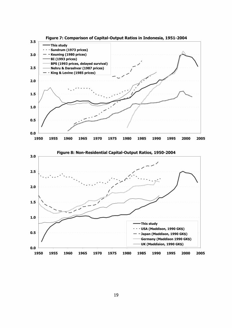
Figure 7: Comparison of Capital-Output Ratios in Indonesia, 1951-2004

0.0

0.5

1.0

1.5

2.0

2.5

3.0

3.5

1950 1955 1960 1965 1970 1975 1980 1985 1990 1995 2000 2005

This studySundrum (1973 prices)Keuning (1980 prices)BI (1993 prices)BPS (1993 prices, delayed survival)Nehru & Darashvar (1987 prices)King & Levine (1985 prices)

Figure 8: Non-Residential Capital-Output Ratios, 1950-2004

0.0

0.5

1.0

1.5

2.0

2.5

3.0

1950 1955 1960 1965 1970 1975 1980 1985 1990 1995 2000 2005

This study

USA (Maddison, 1990 GK$)

Japan (Maddison, 1990 GK$)

Germany (Maddison 1990 GK$)

UK (Maddision, 1990 GK$)

19

20

Appendix Table A1: GFCF in Indonesia, 1951-2004 (bln. 1983 Rupiahs)

Appendix Table A2: GFCS in Indonesia, 1951-2004 (bln. 1983 Rupiah)