Capital Regulation and Monetary Policy

with Fragile Banks∗

Ignazio Angeloni

European Central Bank and BRUEGEL

Ester Faia

Goethe University Frankfurt, Kiel IfW and CEPREMAP

First draft: August 2009. This draft: October 2010.

Abstract

We introduce banks, modeled following Diamond and Rajan ([27], [29]) in a standard DSGE

macromodel and use this framework to study monetary policy transmission and the interplay

between monetary policy and bank capital regulation when banks are exposed to runs. A

monetary expansion, a positive productivity shock or an asset price boom increase bank leverage

and risk. Risk-based capital requirements (Basel II-type) amplify the cycle and are welfare

detrimental. Within a broad class of simple policy rules, the best combination includes mildly

anticyclical capital ratios (as in Basel III) and a response of monetary policy to asset prices or

bank leverage.

Keywords: capital requirements, leverage, bank runs, macro-prudential policy, monetary

policy.

∗An earlier version of this paper appeared in 2009 as Kiel Working paper under the title "A Tale of Two Policies:Prudential Regulation and Monetary Policy with Fragile Banks". We are grateful to seminar participants at the Swiss

National Bank, New York Fed, IMF, Georgetown University, Maryland University, Federal Reserve Board, Institute

for Advanced Studies Vienna, Kiel Institute for the World Economy, National Bank of Hungary, European Central

Bank, Goethe University Frankfurt, Oxford University, Erasmus University Rotterdam for useful comments. Kiryl

Khalmetski and Marc Schöfer provided excellent research assistance. We are the sole responsible for any errors and

for the opinions expressed in this paper.

1

1 Introduction

The financial crisis is producing, among other consequences, a change in perception on the roles

of financial regulation and monetary policy. The pre-crisis common wisdom sounded roughly like

this. Capital requirements and other prudential instruments were supposed to ensure, at least

with high probability, the solvency of individual banks, with the implicit tenet that stable banks

would automatically translate into a stable financial system. On the other side, monetary policy

should largely disregard financial matters and concentrate on pursuing price stability (a low and

stable consumer price inflation) over some appropriate time horizon. The recent experience is

changing this accepted wisdom in two ways. On the one hand, the traditional formal requirements

for individual bank solvency (asset quality and adequate capital) are no longer seen as sufficient for

systemic stability; regulators are increasingly called to adopt a macro-prudential approach1. On

the other, some suggest that monetary policy should help control systemic risks in the financial

sector. This crisis has demonstrated that such risks can have disruptive implications for output and

price stability, and there is growing evidence that monetary policy influences the degree of riskiness

of the financial sector2. These ideas suggest the possibility of interactions between the conduct of

monetary policy and that of macroprudential regulation.

In this paper we study how bank regulation and monetary policy interact in a macroeconomy

that includes a fragile banking system3. To do this we need first a model that rigorously incorporates

state-of-the art banking theory in a general equilibrium macro framework and also incorporates

some key elements of financial fragility experienced in the recent crisis. In our model, whose banking

core is adapted from Diamond and Rajan ([27], [29]), banks have special skills in redeploying

projects in case of early liquidation. Uncertainty in projects outcomes injects risk in bank balance

sheets. Banks are financed with deposits and capital; bank managers optimize the bank capital

structure by maximizing the combined return of depositors and capitalists. Banks are exposed to

runs, with a probability that increases with their deposit ratio or leverage. The relationship between

the bank and its outside financiers (depositors and capitalists) is disciplined by two incentives:

1Morris and Shin [49]; Borio [14]; Lorenzoni[45].2Maddaloni and Peydró Alcalde [46] report evidence of a "risk-taking channel" of monetary policy in the euro

area. For an overview, see Altunbas et al. [5].3We refer to "banks" and "deposits" for convenience, but our arguments apply equally to other leveraged entities

financed through short-term revolving debt like ABSs or commercial paper.

2

depositors can run the bank, forcing early liquidation of the loan and depriving bank capital of its

return; and the bank can withhold its special skills, forcing a costly liquidation of the loan. The

desired capital ratio is determined by trading-off balance sheet risk with the ability to obtain higher

returns for outside investors in "good states" (no run), which increase with the share of deposits

in the bank’s liability side.

Introducing these elements provides a characterization of financial sector that is, we think,

more apt to interpret the recent experience than classic "financial accelerator" formulations which,

although pioneering the introduction of financial frictions into macro models, focussed normally

on the role of firms’ collateral in the transmission of shocks rather than explicitly on banks. En-

dogenizing the bank capital structure also provides a natural way to study banking regulation in

conjunction with monetary and other macro policies. Our model allows, inter alia, to study how

capital regulation, and potentially also liquidity ratios and other prudential instruments, influence

economic performance, collective welfare and the optimal monetary policy.

Blum and Hellwig [13], and Cecchetti and Li [18] have examined optimal monetary policy

design and bank regulation with specific reference to the pro-cyclicality of capital requirements.

Two main elements differentiate our work. First, these studies have taken capital requirements as

given and studied the optimal monetary policy response, while we consider their interaction and

possible combinations. Second, in earlier studies the loan market and bank capital structure were

specified exogenously or ad hoc, while we incorporate optimizing bank behavior explicitly. Gertler

and Karadi [35] and Gertler and Kiyotaki [36] have recently proposed a model with micro-founded

banks. In their work an asymmetric information problem between banks and uninformed investors

is solved through the introduction of an incentive compatibility constraint, which leads to a relation

between bank capital and external finance premia. Our approach to modelling the bank differs in

that we allow for equilibrium bank runs. More importantly, their aim is to look at the effects of

unconventional monetary policies, while we explore the interplay between (conventional) monetary

policy and bank regulation. Their focus is more on crisis management, ours on crisis prevention.

Our bank’s optimal deposit ratio is positively related to: 1) the bank expected return on assets;

2) the uncertainty of project outcomes; 3) the banks’ skills in liquidating projects, and negatively

related to 4) the return on bank deposits. These properties echo the main building blocks of the

3

Diamond-Rajan banking model. The intuition, roughly speaking, is that increases in 1), 2) and 3)

raise the return to outside bank investors of a unitary increase in deposits, the first by increasing

the expected return in good states (no run), the second by reducing its cost in bad states (run), the

third by increasing the expected return relative to the cost between the two states. A higher deposit

rate reduces deposits from the supply side, because it increases, ceteris paribus, the probability of

run. Inserting this banking core into a standard DSGE framework yields a number of results. A

monetary expansion, a positive productivity or an asset price boom increase bank leverage and

risk. The transmission from productivity changes to bank risk is stronger when the riskiness of the

projects financed by the bank is low. Pro-cyclical capital requirements (akin to those implied by

the Basel II internal ratings based approach) amplify the response of output and inflation to other

shocks, thereby increasing output and inflation volatility, and reduce welfare. Conversely, anti-

cyclical ratios, requiring banks to build up capital buffers in more expansionary phases of the cycle,

have the opposite effect. To analyse alternative policy rules we use second order approximations,

which in non-linear models allow to account for the effects of volatility on the mean of all variables,

including welfare. Within a broad class of simple policy rules, the optimal combination includes

mildly anti-cyclical capital requirements (i.e., that require banks to build up capital in cyclical

expansions) and a monetary policy that reacts to inflation and "leans-against-the-wind". Two

alternative forms of “leaning” are examined: a positive response of the policy-determined interest

rate to asset prices or to bank leverage.

The rest of the paper is as follows. Section 2 provides a brief overview of the recent but

rapidly growing literature merging banking into macro models. Section 3 describes the model, with

special emphasis on the banking bloc — our main novelty. Section 4 characterizes the transmission

mechanism. Section 5 examines the sensitivity to some key parameters. Section 6 matches some

properties of the calibrated model with data on the euro area and the US. Sections 7 discusses the

effect of introducing regulatory capital ratios. Section 8 examines the performance of alternative

monetary policy rules combined with different bank capital regimes. Section 9 concludes.

4

2 Merging the Banking and the Macro Literatures

After the financial crisis, considerable attention has been devoted on how to embed credit frictions

and financial risks into macroeconomic analyses. Attempts to take financial frictions into account

pre-existed, but most of the them had focused on credit constraints faced alternatively by house-

holds and firms, without explicitly considering banks or other financial intermediaries. Models of

the financial accelerator family4 studied business cycle fluctuations generated by agency problems

between firms and lenders, while models with collateral constraints along the lines of the Kiyotaki

and Moore [44] focused more on the impact of constraints on households borrowing on the macro

dynamic5. The crisis highlighted the lack of a macro model embedding micro-founded banks. Such

absence prevented both the explicit consideration of financial intermediaries as a source of shocks

to the macroeconomy, and the study of the macroeconomic impact of financial regulation.

Recently, steps have been taken toward integrating banking or financial sectors in infinite

horizon DSGE models, with purposes partially similar to ours. Those papers can be divided in

four main categories, based on a classification pertaining to the finance literature. First, there are

models that include banks facing a single moral hazard problem with the uninformed investors: to

this category belong the papers by Gertler and Karadi [35] and Gertler and Kiyotaki [36], with the

latter also including an interbank market. In this case the moral hazard problem is dealt with by

modeling incentive compatibility constraints of a dynamic nature. The second category includes

models that embed a dual moral hazard problem on the lines of Diamond [25] and Holmström and

Tirole [38]6. The third category includes models analyzing liquidity spirals7. There is then a fourth

category focusing on the industrial structure of the banking sector, in the Klein-Monti tradition8.

Though some of those papers explore the impact of capital regulation and in very few cases also the

interaction with monetary policy, none addresses the issue of bank runs. One of the main feature

of the recent financial crisis, if not the most problematic, has been the possibility of dry up of

4Bernanke and Gertler [35], Bernanke, Gertler and Gilchrist [9], Carlstrom and Fuerst [19], Christiano, Motto and

Rostagno [21]).5See Iacoviello [39].6To this category belong papers by Meh and Moran [47], Covas and Fujita [22], He and Krishnamurthy [37], with

the latter using a continuos time structure. Along the same lines Faia [32] introduces banks and secondary markets

for credit risk transfer into a DSGE model.7See for instance Bunnermeier and Sannikov [17], Iacoviello [40].8See among others Acharya and Naqvi [1], Corbae and D’ Erasmo, Darracq Paries et al. [23].

5

liquidity and of funding to financial intermediaries, despite a very expansionary stance of monetary

policy. Runs did not in general affect traditional deposits (Northern Rock and a few other cases

were exceptions), but typically other more volatile forms of funding for banks and conduits, like

REPOs and ABSs.

To capture these mechanisms, we build on Diamond and Rajan [27], [29], whose models include

both moral hazard considerations and bank runs. Note that, while in this respect we connect to the

literature on bank runs9, our analysis of the interplay between bank runs and liquidity does not lead

to multiplicity of equilibria. We can then study financial and macroeconomic stability issues under

conventional monetary and bank regulatory policies, without making recourse to yet unexplored

equilibrium-selecting instruments. In our model, equilibrium bank runs have distributional effects,

but do not lead to real resource losses nor affect the long run equilibrium10.

Diamond and Rajan [28] provide a first attempt to integrate banks and bank runs in a monetary

model. They do so in a two period economy model in which monetary policy is conducted by means

of money supply and monetary non-neutrality is obtained via frictions on deposits. They find that

monetary policy should inject money during contractionary phases. Our analysis includes banks

into an infinite horizon DSGE model hence it accommodates the role of expectations and accounts

for the Lucas critique. Moreover, our paper includes the study of the optimal combination of

prudential regulation and monetary policy, alongside with an analysis of the monetary transmission

mechanism.

3 The Baseline Model

The starting point is a conventional DSGE model with nominal rigidities. There are four type

of agents in this economy: households, financial intermediaries, final good producers and capital

producers. The model is completed by a monetary policy function (a Taylor rule) and a skeleton

fiscal sector.

9Diamond and Dybvig [26], Allen and Gale [2],[3],[4].10Angeloni, Faia and Lo Duca [6] consider an extension of our model which includes the cost of runs. Such feature

does not alter qualitatively the results obtained in this paper.

6

3.1 Households

There is a continuum of identical households who consume, save and work. Households save by

lending funds to financial intermediaries, in the form of deposits and bank capital. To allow

aggregation within a representative agent framework we follow Gertler and Karadi [35] and assume

that in every period a fraction of household members are bank capitalists and a fraction (1−) areworkers/depositors. Hence households also own financial intermediaries11. Bank capitalists remain

engaged in their business activity next period with a probability which is independent of history.

This finite survival scheme is needed to avoid that bankers accumulate enough wealth to remove the

funding constraint. A fraction (1− ) of bank capitalists exit in every period, and a corresponding

fraction of workers become bank capitalists every period, so that the share of bank capitalists,

remains constant over time. Workers earn wages and return them to the household; similarly

bank capitalists return their earnings to the households. However, bank capitalists’ earnings are

not used for consumption but are given to the new bank capitalists and reinvested as bank capital.

Consumption and investment decisions are made by the household, pooling all available resources.

As will be described later, the bank capital structure is determined by bank managers, who

maximize the returns of both depositors and bank capitalists. Bank managers are workers in the

financial sector. Hence, household members can either work in the production sector or in the

financial sector. We assume that the fraction of workers in the financial sector is negligible, hence

their earnings are not included in the budget constraint.

Households maximize the following discounted sum of utilities:

0

∞X=0

( ) (1)

where denotes aggregate consumption and denotes labour hours. The workers in the

production sector receive at the beginning of time a real labour income

Households save and invest in bank deposits and bank capital. Deposits, pay a gross

nominal return one period later. Households also own the production sector, from which they

receive nominal profits for an amount, Θ. Let be net transfers to the public sector (lump sum

11As in Gertler and Karadi [35] it is assumed that households hold deposits with financial intermediaries that they

do not own.

7

taxes, equal to public expenditures); the budget constraint reads as follows:

+ ++1 ≤ +Θ + (2)

Note that the return from, and the investment in, bank capital do not appear in equation

2. The reason is that we have assumed, as explained later, that all returns on bank capital are

reinvested every period.

Households choose the set of processes ∞=0 and deposits +1∞=0 taking as giventhe set of processes ∞=0 and the initial value of deposits 0 so as to maximize 1 subject

to 2. The following optimality conditions hold:

= −

(3)

= +1 (4)

Equation 3 gives the optimal choice for labour supply. Equation 4 gives the Euler condition

with respect to deposits. Optimality requires that the first order conditions and No-Ponzi game

conditions are simultaneously satisfied.

3.2 Banks

There is in the economy a large number () of uncorrelated investment projects. The project lasts

two periods and requires an initial investment. Each project’s size is normalized to unity (think

of one machine) and its price is . The projects require funds, which are provided by the bank.

Banks have no internal funds but receive finance from two classes of agents: holders of demand

deposits and bank capitalists. Total bank loans (equal to the number of projects multiplied by

their unit price) are equal to the sum of deposits () and bank capital, (). The aggregate

bank balance sheet is:

= + (5)

The capital structure (deposit share, equal to one minus the capital share) is determined by

bank manager on behalf of the external financiers (depositors and bank capitalists). The manager’s

8

task is to find the capital structure that maximizes the combined expected return of depositors and

capitalists, in exchange for a fee. Individual depositors are served sequentially and fully as they come

to the bank for withdrawal; bank capitalists instead are rewarded pro-quota after all depositors

are served. This payoff mechanism exposes the bank to runs, that occur when the return from

the project is insufficient to reimburse all depositors. As soon as they realize that the payoff is

insufficient, depositors run the bank and force the liquidation of the project; in this case the bank

capital holders get zero while depositors get the market value of the liquidated loan.

The timing is as follows. At time , the manager of bank decides the optimal capital structure,

expressed by the ratio of deposits to total loans, =

, collects the funds, lends, and then

the project is undertaken. At time +1, the project’s outcome is known and payments to depositors

and bank capitalists (including the fee for the bank manager) are made, as discussed below. A new

round of projects starts.

Generalizing Diamond and Rajan [27], [29], we assume that the return of each project for the

bank is equal to an expected value, , plus a random shock, for simplicity assumed to have a

uniform density with dispersion (the assumption yields a convenient closed form solution but is

not essential for our results; see Appendix 1). Therefore, the outcome of project is + ,

where spans across the interval [−;] with probability 12. We assume to be constant across

projects and time, but will run sensitivity analyses on its value.

Given our assumption of identical projects and banks, for notational convenience from now

on we can omit project and bank subscripts. In this subesection and the next, we will omit time

subscript as well.

Each project is financed by one bank. Our bank is a relationship lender : by lending it acquires

a specialized non-sellable knowledge of the characteristics of the project. This knowledge determines

an advantage in extracting value from it before the project is concluded, relative to other agents.

Let the ratio of the value for the outsider (liquidation value) to the value for the bank be 0 1.

Again we assume to be constant, but we will examine the sensitivity of the results to changes in

its value.

Suppose the ex-post realization of is negative, as depicted in Graph 1 (point C), and consider

how the payoffs of the three players are distributed depending on the ex-ante determined value of

9

the deposit ratio and the deposit rate .

There are three cases.

Case A: Run for sure. The outcome of the project is too low to pay depositors. This happens

if gross deposits (including interest) are located to the right of C in the graph, where + .

Payoffs are distributed as follows. Capitalists receive the leftover after depositors are served, so

they get zero in this case. Depositors alone (without bank) would get the fraction (+) of the

project’s outcome (segment AB), so they claim this amount in full. The remainder (1−)(+) is

shared between depositors and the bank depending on their relative bargaining power. As Diamond

and Rajan [27], we assume this extra return is split in half 12. Therefore, depositors end up with

(1+)(+)2

and the bank with(1−)(+)

2.

Note that we have assumed that bank runs do not destroy value per se, but only affect the

distribution of returns. The model can easily be extended to include a specific deadweight loss

from bank runs. Intuitively, the higher such loss, the lower the equilibrium deposit ratio, but the

main properties of the model remain unchanged.

Case B: Run only without the bank. The project outcome is high enough to allow depositors

to be served if the project’s value is extracted by the bank, but not otherwise. This happens if

gross deposits (including interest) are located in the segment BC in the graph, i.e. the range where

( + ) ≤ ( + ). In this case, the capitalists alone cannot avoid the run, but with the

bank they can. So depositors are paid in full, , and the remainder is split in half between the

banker and the capitalists, each getting +−2

. Total payment to outsiders is ++2

.

Case C: No run for sure. The project’s outcome is high enough to allow all depositors to

be served, with or without the bank’s participation. This happens in the zone AB, where ≤( + ). Depositors get . However, unlike in the previous case, now the capitalists have

a higher bargaining power because they could decide to liquidate the project alone and pay the

depositors in full, getting (+ )−; this is thus a lower threshold for them. The banker can

extract (+)−, and again we assume that the capitalist and the bank split this extra return12 It seems natural to assume that depositors and bank managers have equal bargaining power because neither can

appropriate the extra rent without help from the other. But, as shown in Appendix 1, thi asumption is not crucial.

Diamond and Rajan [27] mention also another case in which the depositors, after appropriating the project, bargain

directly with the entrepreneur running the project. If the entrepreneur retains half of the rent, the result is obviously

unchanged. If not, the resulting equilibrium is more tilted towards a high level of deposits, because depositors lose

less in case of bank run.

10

in half. Therefore, the bank gets:

[( + )−]− [( + )−]

2=(1− )( + )

2

This is less than what the capitalist gets. Total payment to outsiders is:

(1 + )( + )

2

We can now write the expected value of total payments to outsiders as follows:

1

2

⎡⎢⎢⎣−Z−

(1 + )( + )

2+

−Z

−

( + ) +

2+

Z−

(1 + )( + )

2

⎤⎥⎥⎦ (6)

The three terms express the payoffs to outsiders in the three cases described above, in order.

The banker´s problem is to maximize expected total payments to outsiders by choosing the suitable

value of .

Proposition 1. The value of that maximizes equation 6 is comprised in the interval

+

+.

Proof. See Appendix 1.

In this zone, the third integral in the equation vanishes and the expression reduces to

1

2

−Z−

(1 + )( + )

2+

1

2

Z−

( + ) +

2 (7)

Consider equation 7 in detail. A marginal increase in the deposit ratio has three effects. First,

it increases the range of where a run occurs, by raising the upper limit of the first integral; this

effect increases the overall return to outsiders by 12

¡1+2¢. Second, it decreases the range of

where a run does not occur, by raising the lower limit of the second integral; the effect of this on the

return to outsiders is negative and equal to − 122. Third, it increases the return to outsiders for

each value of where a run does not occurs; this effect is 12

⎛⎜⎝ Z−

12

⎞⎟⎠ = 12

³−+

2

´.

11

Equating to zero the sum of the three effects and solving for yields the following solution for the

level of deposits for each unit of loans

=1

+

2− (8)

Since the second derivative is negative, this is the optimal value of .

The optimal deposit ratio depends positively on , and , and negatively on . An increase

of reduces deposits because it increases the probability of run. Moreover, an increase in raises

the marginal return in the no-run case (the third effect just mentioned), while it does not affect

the other two effects, hence it raises . An increase in reduces the cost in the run case (first

effect), while not affecting the others, so it raises . The effect of is more tricky. At first sight it

would seem that an increase in the dispersion of the project outcomes, moving the extreme values

of the distribution both upwards and downwards, should be symmetric and have no effect. But

this is not the case. When increases, the probability of each given project outcome 12falls.

Hence the expected loss stemming from the change in the relative probabilities (sum of the first

two effects) falls, but the marginal gain in the no-run case (third term) does not, because the upper

limit increases. The marginal effect is 2, because depositors get the full return, but half is lost by

the capitalist to the banker. Hence, the increase of has on a positive effect, as .

In the aggregate, the amount invested in every period is = . The total amount of

deposits in the economy is =

+

2− and aggregate bank capital is

= (1− 1

+

2− ) (9)

The latter expressions suggest that following an increase in the optimal amount of bank

capital increases on impact (for given ). In general equilibrium the responses are more complex,

depending on several counterbalancing factors affecting and , as the later results will show.

3.2.1 A measure of bank fragility

A natural measure of bank riskiness is the probability of a run occurring. This can be written as:

12

=1

2

−Z−

=1

2

µ1− −

¶=1

2− (1− )−

2(2− )(10)

Graph 2 shows the shape of the last function in 10 for = 103). Note that for low values of

and , +2− falls below + and the marginal equilibrium condition 8 and the last equality

of 10 cease to hold. Deposits can never fall below the level where a run becomes impossible. Some

degree of bank risk is always optimal in this model.

0.0

0.2

0.4

bank risk

0.6

0.8

1.0

1.0

0.6

h

0.6

0.8 0.4lambda

0.4 0.8

1.0

Graph 2

3.2.2 Accumulation of bank capital

Equation 9 is the level of bank capital desired by the bank manager, for any given level of investment,

and interest rate structure (, ). We assume that bank capital is provided by the bank

capitalist. After remunerating depositors and paying the competitive fee to the bank manager, a

return accrues to the bank capitalist, and this is reinvested in the bank as follows:

= [−1 +] (11)

13

where is the unitary return to the capitalist. The parameter is a decay rate, given by

the bank survival rate already discussed. can be derived from equation 7 as follows:

=1

2

Z−

( + )−

2 =

( + −)2

8(12)

Note that this expression considers only the no-run state because if a run occurs the capitalist

receives no return. The accumulation of bank capital is obtained substituting 12 into 11:

= [−1 +( + −)

2

8] (13)

Importantly, notice that booms and busts in asset prices, also affect bank capital. This

captures the balance sheet channel in our model.

3.3 Producers

Each firm has monopolistic power in the production of its own variety and therefore has leverage

in setting the price. In changing prices it faces a quadratic cost equal to 2(

()

−1()− 1)2 where

the parameter measures the degree of nominal price rigidity13. The higher , the more sluggish

is the adjustment of nominal prices. In the particular case of = 0 prices are flexible. Each

firm assembles labour and (finished) entrepreneurial capital to operate a constant return to scale

production of the variety of the intermediate good:

() = (()()) (14)

Each monopolistic firm chooses a sequence () () () taking nominal wage rates and the rental rate of capital as given, in order to maximize expected discounted nominal

profits:

0∞X=0

Λ0[()()− (() + ())−

2

∙()

−1()− 1¸2

] (15)

subject to the constraint (•) ≤ (), where Λ0 is the households’ stochastic discount

factor.

13Alternative assumptions, such as adjustment costs on deposits, would yield similar results.

14

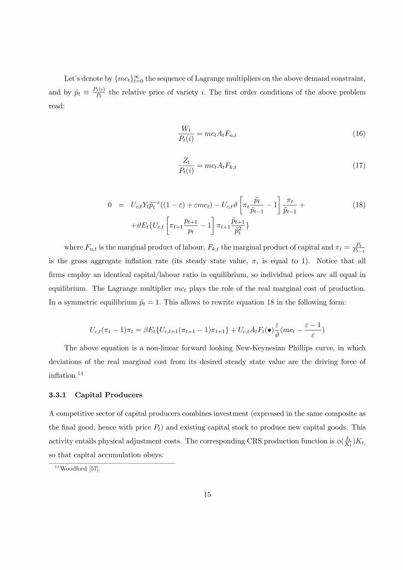
Let’s denote by ∞=0 the sequence of Lagrange multipliers on the above demand constraint,and by ≡ ()

the relative price of variety The first order conditions of the above problem

read:

()= (16)

()= (17)

0 = − ((1− ) + )−

∙

−1− 1¸

−1+ (18)

+

∙+1

+1

− 1¸+1

+1

2

where is the marginal product of labour, the marginal product of capital and =

−1

is the gross aggregate inflation rate (its steady state value, , is equal to 1). Notice that all

firms employ an identical capital/labour ratio in equilibrium, so individual prices are all equal in

equilibrium. The Lagrange multiplier plays the role of the real marginal cost of production.

In a symmetric equilibrium = 1 This allows to rewrite equation 18 in the following form:

( − 1) = +1(+1 − 1)+1+ (•) ( − − 1

)

The above equation is a non-linear forward looking New-Keynesian Phillips curve, in which

deviations of the real marginal cost from its desired steady state value are the driving force of

inflation.14

3.3.1 Capital Producers

A competitive sector of capital producers combines investment (expressed in the same composite as

the final good, hence with price ) and existing capital stock to produce new capital goods. This

activity entails physical adjustment costs. The corresponding CRS production function is ( )

so that capital accumulation obeys:

14Woodford [57].

15

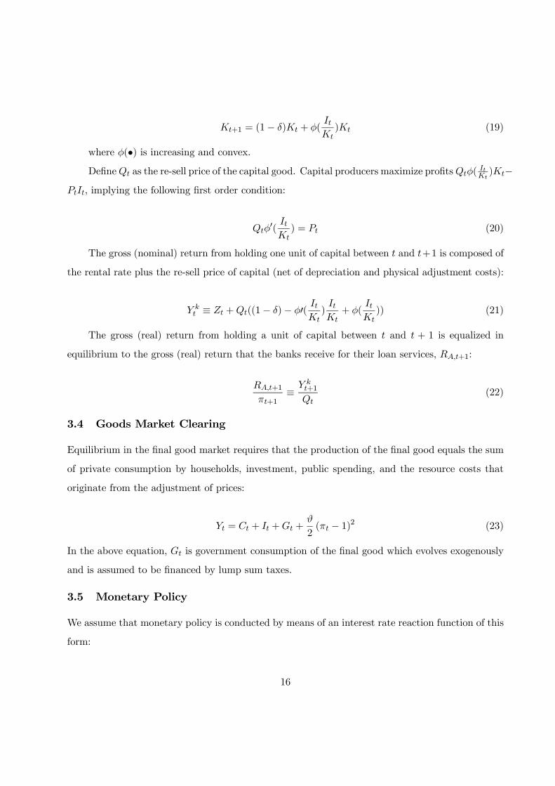
+1 = (1− ) + (

) (19)

where (•) is increasing and convex.Define as the re-sell price of the capital good. Capital producers maximize profits(

)−

implying the following first order condition:

0(

) = (20)

The gross (nominal) return from holding one unit of capital between and +1 is composed of

the rental rate plus the re-sell price of capital (net of depreciation and physical adjustment costs):

≡ +((1− )− 0(

)

+ (

)) (21)

The gross (real) return from holding a unit of capital between and + 1 is equalized in

equilibrium to the gross (real) return that the banks receive for their loan services, +1:

+1

+1≡

+1

(22)

3.4 Goods Market Clearing

Equilibrium in the final good market requires that the production of the final good equals the sum

of private consumption by households, investment, public spending, and the resource costs that

originate from the adjustment of prices:

= + + +

2( − 1)2 (23)

In the above equation, is government consumption of the final good which evolves exogenously

and is assumed to be financed by lump sum taxes.

3.5 Monetary Policy

We assume that monetary policy is conducted by means of an interest rate reaction function of this

form:

16

ln

µ

¶= (1− )

∙ ln

³

´+ ln

µ

¶+ ln

µ

¶+ ln∆

µ

¶¸(24)

+ ln

µ−1

¶All variables are deviations from the target or steady state (symbols without time subscript).

Note that the reaction function includes two alternative terms that express leaning-against-the-wind

behavior, in the form of a response to asset prices () or to the change of the deposit ratio (). We

will compare policy rules of this form, characterized by different parameter sets . We solve the model by computing a second order approximation of the policy functions around

the non-stochastic steady state.

3.6 Parameter values

Household preferences and production. The time unit is the quarter. The utility function of house-

holds is ( ) =1− −11− + log(1−) with = 2 as in most real business cycle literature.

We set set equal to 3, chosen in such a way to generate a steady-state level of employment

≈ 03. We set the discount factor = 0995, so that the annual real interest rate is around 2%.We assume a Cobb-Douglas production function (•) =

()1− with = 03 The quarterly

aggregate capital depreciation rate is 0.025, the elasticity of substitution between varieties 6. The

adjustment cost parameter is set so that the volatility of investment is larger than the volatility of

output, consistently with empirical evidence: this implies an elasticity of asset prices to investment

of 2. The price stickiness parameter is set equal to 30, a value that matches, in the Rotem-

berg framework, the empirical evidence on the frequency of price adjustments obtained using the

Calvo-Yun approach15.

Banks. To calibrate we have calculated the average dispersion of corporate returns from the

data constructed by Bloom et al. [12], which is around 0.3, and multiplied this by the square root

of 3, the ratio of the maximum deviation to the standard deviation of a uniform distribution. The

result is 0.5. We set the value of slightly lower, at 0.45, a number that yields a more accurate

15See Gali and Gertler [34] and Sbordone [53]. The New Keynesian literature has usually considered a frequency of

price adjustment of four quarters as realistic. Recently, Bils and Klenow [10] have argued that the observed frequency

of price adjustment in the US is higher, in the order of two quarters.

17

estimates of the steady state values of the bank deposit ratio16, and then run sensitivity analyses

above and below this value17.

One way to interpret is to see it as the ratio of two present values of the project, the first at the

interest rate applied to firms’ external finance, the second discounted at the bank internal finance

rate (the money market rate). A benchmark estimate can be obtained by taking the historical ratio

between the money market rate and the lending rate. In the US over the last 20 years, based on

30-year mortgage loans, this ratio has been around 3 percent. This leads to a value of around 0.6.

In the empirical analyses we have chosen 0.45 and then run sensitivity analyses above and below

this value.

Finally we parametrize the survival rate of banks, at 0.97, a value compatible with an average

horizon of 10 years. Notice that the parameter (1− ) is meant to capture only the exogenous exit

rates, as the failure rate is linked to the distribution of the idiosyncratic shock to corporate returns.

Shocks. Total factor productivity is assumed to evolve as an AR(1) process, = −1 exp(

),

where the steady-state value is normalized to unity (which in turn implies = 1) and where

is an i.i.d. shock with standard deviation In line with the real business cycle literature, we

set = 095 and = 0056. Log-government consumption is assumed to evolve according to the

process ln(

) = ln(

−1) +

, where is the steady-state share of government consumption

(set in such a way that = 025) and

is an i.i.d. shock with standard deviation We follow

the empirical evidence for the U.S. in Perotti [50] and set = 00074 and = 09

We introduce a monetary policy shock as an additive disturbance to the interest rate set

through the monetary policy rule. The monetary policy shock is assumed to be moderately persis-

tent (coefficient 0.2), as argued by Rudebusch [52]. Based on the evidence of Angeloni, Faia and Lo

Duca [6], and consistently with other empirical results for US and Europe, the standard deviations

of the shocks is set to 0006.

16The bank capital accumulation equation 13, once we substitute in the optimal deposit ratio 8, yields a quadratic

equation in . Solving the quadratic equation for given values of the parameters, one obtains a root for equal

to 1.03 (3 percent on a quarterly basis). The corresponding value of is 95 percent, and is 5 percent. Notice that

the bank capital accumulation equation includes the money that households transfer in every period to new bankers,

given by a fraction of the value of the project: The steady state value that helps to pin down the return on

asset, is 0.075. Since such term is negligible we have omitted that in the dynamic.17 In principle, could be endogenous to the state of the economy; recent work by Bloom ([11], [12]) has shown that

the dispersion of corporate returns is anticyclical. A link between and the cycle could be added into our framework.

In this paper we have used a fixed and done sensitivity analysis.

18

4 Transmission Channels

We first look at the response of the model to three shocks: a one-time total factor productivity

rise; a monetary restriction; a positive shock to the marginal return on capital (MRK), interpreted

as a positive asset price shock.

As common in DSGE models with nominal rigidities, a positive productivity shock (figure 1)

reduces inflation and increases output. The increase in productivity also brings about an increase

in capital and investment. The ensuing increase in the asset price reduces the return on bank

assets, The policy-driven short term interest rate, falls, as the monetary authority reacts

to the fall in inflation by means of a Taylor rule. The lower interest rates raise deposits and tilt

the composition of the bank balance sheet towards higher leverage and risk.

In the monetary shock (figure 2) both, inflation and output, drop on impact, as in all standard

models, with a corresponding fall in investment and Tobin’s Q. The reduction in the asset price

activates the balance sheet channel and induces an increase in the return to capital, Also the

spread between and rises, but this is sensitive to parameter values — generally speaking,

with a persistent shock or with interest rate smoothing, the spread tends to rise after a monetary

restriction. Banks lose deposits and replace them with capital, leading to a less risky balance sheet

composition; bank riskiness drops on impact — a "risk taking channel" of monetary policy operating

in reverse.

Figure 3 shows the response of the selected variables to a positive asset market shock, which is

modeled as an AR(1) shock to the return to capital. The increase in brings about an increase

in investment. As a consequence of the increase in capital, output rises. The interest rate,

broadly follows the dynamics of inflation. Bank risk declines, despite the high deposit ratio, due

to the rise in the spread between and .

The above results together suggest that the co-movements of bank risk on one side, and interest

rates and output on the other, depend on the nature of the shock. Higher policy-driven interest rates

lead to lower bank risk, but not if there is a concurrent investment boom, for example generated

by asset market exuberance. In this case banks become more risky in spite of higher policy rates.

19

5 Sensitivity to Key Parameters

5.1 Bank liquidation skills

To examine how banks affect the transmission, we compare two models, one with benchmark

parameters, the other obtained setting = 065. A higher value of means that banks lose some

of their advantage as relationship lenders. In figure 4, constructed assuming a TFP shock, the

response from the standard model with banks is shown with a solid line, that from the model with

higher with a dashed line. We can see that a low amplifies the short run expansionary effect

on output. The reason is that the decline in ROA, the key transmission variable from the banking

to the real sector in our model, is larger in the short run.

5.2 Entrepreneurial risk

Entrepreneurial risk is distinct from bank risk: the first is measured by the parameter , while the

second depends endogenously on the bank capital structure. The two are linked, however: a higher

tends to increase the bank leverage and the probability of run on the bank , as one can see in

equation 10 and graph 2 attached to it. Moreover, also affects the response of the bank capital

structure and risk to all other shocks.

Figures 5 and 6 report the responses to a TFP and a monetary shock respectively, with values

of equal to 0.45, the baseline, and 0.65, an alternative in which the entrepreneurial risk is higher.

Under the positive productivity shock, the short run response of output, capital, credit and

investment is stronger if the value of is lower. This highlights a self-reinforcing mechanism that

may operate in "exuberant" phases: positive productivity shocks are more expansionary if the

perception of investment risk is low.

Under a monetary restriction, on the contrary, the business cycle response is amplified in the

high risk case; we have a bigger drop in output, investment and capital, together with a sharper

fall in bank leverage. This is due to the fact that the downward effect of a given change in the

interest rate on the deposit ratio is stronger when is high (see equation 8), hence in presence of a

stronger need for bank capital rises more on impact and the transmission to investment and

output is higher.

By contrast, however, under a monetary shock the impact on bank riskiness is smaller when

20

entrepreneurial risk is higher (a high dampens the stronger increase in in equation 10). This

means that the risk taking channel of monetary policy impacts more strongly when the ex-ante

uncertainty of projects is low (this effect involving two factors, and the interest rate, should not

be confused with the fact that bank risk increases when entrepreneurial risk rises, as we have

already noted). This observation connects with the earlier one concerning "exuberant" states; in

these situations, an overly expansionary monetary policy tends to have particularly strong effects

on bank leverage, exacerbating the increase of bank risk. Since the empirical evidence shows that

entrepreneurial risk tends to be anti-cyclical, we conclude that the strength of the risk taking

channel depends on the cyclical position. An expansionary monetary policy when the economy is

strong increases bank risk by more than the same policy when the economy is weak.

5.3 Leaning against the wind

Figure 7 compares the benchmark monetary policy rule with two strategies in which the interest

rate reacts also to asset prices (more precisely Tobin’s Q, with a coefficient of 0.5) or alternatively

to bank leverage (the change in the deposit ratio, with the same coefficient). We regard these

as alternative options of using monetary policy (also) to control risks in the financial sector by

leaning-against-the-wind in financial markets. Comparing these alternatives can contribute new

elements to the old debate on whether monetary policy should react to expected inflation only (see

Bernanke and Gertler [7]) or to asset prices as well (Cecchetti, Genberg, Lipsky and Whadwani

[20]). Since one argument in that debate was that responding to asset prices would inject volatility

in the economy, it is interesting to look at an alternative measure based on bank balance sheets,

that should be empirically more stable.

The figure is constructed assuming an asset price shock. As one can see, the two strategies

give mixed results. The rule that reacts to Tobin Q is successful in stabilizing inflation and to

some extent also output, but on bank risk and the deposit ratio the result is less clear. Reacting to

leverage instead does not seem to improve the performance relative to a standard Taylor rule, and

in some cases (on output and inflation for example) the performance is actually worse. All in all,

the results speak in favor of responding to asset prices, not leverage. But this result is obtained

under a single shock only. As we shall see later, using a broader set of calibrated shocks tends to

tilt the balance in favor of responding to leverage in some cases.

21

6 Matching the Data

Before introducing regulatory bank capital requirements and turning to the analysis of optimal

policy it is useful to compare the quantitative properties of our model with the data. We do so by

comparing a series of statistics (standard deviation and first order autocorrelation) generated by

our model with the data equivalent18.

We look at data for both the US and the euro area for the following variables: output, con-

sumption, investment, employment, the deposit rate, the return on assets, the deposit ratio, and

bank riskiness. Deposit rates for the US are average rates on all deposits included in M2; for the

euro area, average rates on short and long term deposits. Lending rates for the US are proxied by

the 6-month commercial paper rate, for the euro area by the average rate on loans to households and

non-financial corporations. To proxy the deposit ratio, which in the model measures bank balance

sheet risk, departing from common practice we use the ratio of total bank assets to total deposits.

As argued in Angeloni, Faia and Lo Duca [6], this is a better proxy of balance sheet risk when the

coverage of deposit insurance is large. Insured deposits have increasingly acquired, in recent years,

the nature of stable source of funding for banks, in contrast with other more volatile instruments

(REPOs, short term ABCP, structured products, etc.). The ratio of total assets to total deposits

is a measure of the incidence of these volatile sources of funding in the bank balance sheet. Finally,

bank risk is measured by aggregate default probability measures provided by Moody’s KMV19.

The model equivalent statistics are computed by considering the three fundamental shocks

to productivity, government expenditure and monetary policy. Shocks have been parametrized as

described in the calibration section. Standard deviations and first order autocorrelation, for both

the model and the data, are summarized in table 1. For the comparison we have standardized

the volatility of output to 1 percent, and we have computed the standard deviations for the other

18All data are quarterly and seasonally adjusted where necessary. Euro area aggregates are reconstructed backward

using the available subsets of countries, with the multiplicative method. All variables are detrended before calculating

standard deviations and autocorrelation, using a Hodrick-Prescott filter. Our main sources of data were, for the US,

the St. Louis Fed website and for the euro area the ECB.19Data samples vary according to availability; for the euro area, national accounts data were reconstructed back

since 1963, while most banking variables start in the 1970s or early 1980s. For the US, the starting date is generally

1970 or, for interest rates, the late 1950s. All data series end with the most recent available quarter, normally 2010Q1.

Notice that we have included the crisis period since our model permits the existence of bank runs in equilibrium,

though our data samples are evidently referring to normal (non crisis) market situations.

22

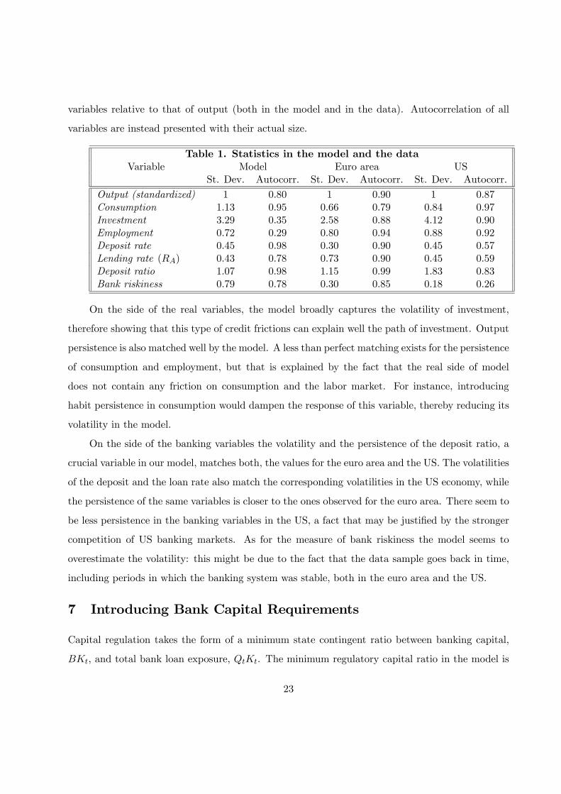
variables relative to that of output (both in the model and in the data). Autocorrelation of all

variables are instead presented with their actual size.

Table 1. Statistics in the model and the data

Variable Model Euro area US

St. Dev. Autocorr. St. Dev. Autocorr. St. Dev. Autocorr.

Output (standardized) 1 080 1 090 1 087

Consumption 113 095 066 079 084 097

Investment 329 035 258 088 412 090

Employment 072 029 080 094 088 092

Deposit rate 045 098 030 090 045 057

Lending rate () 043 078 073 090 045 059

Deposit ratio 107 098 115 099 183 083

Bank riskiness 079 078 030 085 018 026

On the side of the real variables, the model broadly captures the volatility of investment,

therefore showing that this type of credit frictions can explain well the path of investment. Output

persistence is also matched well by the model. A less than perfect matching exists for the persistence

of consumption and employment, but that is explained by the fact that the real side of model

does not contain any friction on consumption and the labor market. For instance, introducing

habit persistence in consumption would dampen the response of this variable, thereby reducing its

volatility in the model.

On the side of the banking variables the volatility and the persistence of the deposit ratio, a

crucial variable in our model, matches both, the values for the euro area and the US. The volatilities

of the deposit and the loan rate also match the corresponding volatilities in the US economy, while

the persistence of the same variables is closer to the ones observed for the euro area. There seem to

be less persistence in the banking variables in the US, a fact that may be justified by the stronger

competition of US banking markets. As for the measure of bank riskiness the model seems to

overestimate the volatility: this might be due to the fact that the data sample goes back in time,

including periods in which the banking system was stable, both in the euro area and the US.

7 Introducing Bank Capital Requirements

Capital regulation takes the form of a minimum state contingent ratio between banking capital,

, and total bank loan exposure, . The minimum regulatory capital ratio in the model is

23

given by following iso-elastic function:

≡

= + 0

µ

¶1

(25)

In Appendix 2 we show that equation 25 mimics very well the minimum capital requirement

implied by the internal ratings based (IRB) approach of Basel II, for appropriate values of the

constant, 0 and 1. Specifically, a negative value of 1 implies that the minimum capital ratio

decreases with the output gap; since the average riskiness of bank loans tends to be negatively

correlated with the cycle (see Appendix 2 for estimates), one can calibrate 1 so that equation 25

reproduces, for each value of the output gap, the capital requirement under the IRB approach,

in which the minimum capital ratio increases with the riskiness of the bank’s loan portfolio. For

1 = 0, equation 25 reproduces the Basel I regime, in which the capital ratio is fixed 20. Setting

positive value of 1 one can study the implications of a hypothetical regime that, following the

current discussions about reforming Basel II, requires banks to accumulate extra capital buffers

when the economy is booming.

In presence of a minimum capital ratio, banks determine their actual capital by optimally

setting the risk that, after the stochastic component of their asset side is realized, their capital

buffer net of losses may fall below the required ratio. The distinction between actual, regulatory

and economic capital (the latter being the optimal capital set by the bank in absence of regulation)

is analyzed by Elizaldea and Repullo [51] in the context of a partial equilibrium banking model.

In our framework, the actual bank capital ratio under regulation is determined extending

equation 6 as follows

1

2

+ −Z−

(1 + )( + )

2 +

1

2

+

−Z

+ −

( + ) +

2 +(26)

+1

2

Z+

−

(1 + )( + )

2

20 In fact, it has been noted that capital regulation is slightly procyclical also under Basel I, due to a number of

accounting and other factors. We disregard this.

24

Note that the intervals of integration are adjusted to take into account. Following the

same procedure seen earlier it is straightforward to show that the internal optimum is given by

= +1

1−

2−

(27)

where is the economic capital. Note that for intermediate values of (close to 0.5) the

coefficient of on the r.h.s. is close to one third; hence

unless is

much higher than In other words, if the capital constraint is not too tight, banks will normally

maintain extra capital above the minimum required, a point stressed by Elizaldea and Repullo [51].

This range, where the capital constraint is not binding (though it does affect the bank’s capital) is

represented by the segment AB in graph 3. The actual deposit ratio in this case is given by

= − 1

1−

2−

=1

+

2− − 1

1−

2−

a lower value than in the absence of constraint (i.e. when = 0), as one would expect.

Only when the capital requirement is sufficiently high (segment BC in the graph below) it will be

strictly binding, i.e. the actual capital ratio set ex-ante will coincide with the regulatory minimum.

The threshold is =

1− 1

+

2−1− 1

1−2−

=(2−)−(+)

(2−)−(1−) . As shown in the graph, above this value

= (28)

A

B

C

bk R 2ΛRAh

R 2Λ1Λ

bkMIN

bk

bkACT

Graph 3

25

In addition to replacing with 27 or 28, depending on the regime, we need to modify the

bank capital accumulation equation 13. In the non strictly binding regime, solving 26 for the return

of the capitalist and substituting in the accumulation equation we get:

= [−1 +( + −

)2 − (

)2

8] (29)

which, we one can easily see, reduces to the standard accumulation equation for = 0.

In the strictly binding regime:

= [−1 +[ + −(1−

)]2

8]

Figure 8 and 9 show respectively, under our usual productivity shock, the responses of the

model under the first regime (where capital is optimized by the bank and the constraint is not

strictly binding) and the second regime (capital constraint strictly binding). In each figure, the

parameters are calibrated so as to mimic three alternative regimes (see Appendix 2 for numerical

details); in the first the required capital ratio is fixed (as in Basel I); in the second it is moves

anticyclically (decreasing when output is above potential, hence producing pro-cyclical macroeco-

nomic effects), as in Basel II21; as our third case, we consider the performance of a hypothetical

regime where the cyclical property of the capital requirement is opposite to that under Basel II, as

determined by inverting the sign of the exponent 1; we refer to this regime as "Basel III"22.

In figure 8 we see that the Basel II regime results in a strong amplification of the short run

effect of the shock on all variables in the model. The amplification is particularly evident on output,

investment and employment, but also bank leverage and risk react more under this shock in a Basel

II environment. Conversely, the Basel III regime implies a more moderate response of the macro

and banking variables, relatively to Basel I, as it turns out that the profile of response under Basel

21Kashyap and Stein [41] report very different estimates of the degree of procyclicality of Basel II, depending on

methodologies, data, etc. What seems to be very robust is the sign — Basel II is clearly procyclical in the sense that

the capital requirements on a given loan pool increase more, when the economy decelerates, relative to what they did

under Basel I.22This terminology is used here for convenience only. In fact, the bew capital accord recently agreed by the Basel

committee on bank supervision, commonly referred to as Basel III, includes, in addition to an anticyclical capital

surcharge, also a significant increase in the average capital requirements. We neglect this element here.

26

I is rather similar to that observed in the absence of capital regulation. Basel III is quite effective in

insulating the effects of the shock on the balance sheet and on the riskiness of the banking system.

Comparing figure 9, where the constraint is strictly binding, we see that a rigid constraint

results in rather sharp movements in the macro variables, which oscillate before returning to the

steady state23. The cyclical amplification is much sharper under Basel II, consistently with the

results in the previous figure. Note that the presence of capital regulation, though having the

possibly undesirable effect of accentuating the business cycle, is actually successful in containing

bank risk: specifically, under a fixed capital ratio bank risk oscillates less not only relative to Basel

II, but also (though this is not shown in the figure) relative to the case in which there is absence of

capital regulation. The stabilizing properties of the "Basel III" case, where banks are required to

build up capital buffers when the cyclical position of the economy is strong, and vice versa in case

of economic slowdown, are quite evident under all types of shock; not only the one shown here —

we omit to report this evidence for brevity. This is true both in the case where banks are strictly

constrained by capital regulation, and in the "soft binding" case illustrated earlier in which they

maintain a buffer above the regulatory minimum.

8 Optimal Monetary Policy and Bank Capital Regulation

We compare the performance of alternative policy combinations using three criteria: household

welfare, output volatility and inflation volatility. Household welfare, calculated from the utility

function, is clearly the most internally consistent criterion. Output and inflation volatilities are

alternative, ad hoc but frequently used, measures of policy performance.

Some observations on the computation of welfare are in order. First, we cannot safely rely on

first order approximations to compare the welfare associated to monetary policy rules, because in an

economy with time-varying distortions stochastic volatility affects both first and second moments24.

Since in a first order approximation of the model solution the expected value of a variable coincides

with its non-stochastic steady state, the effects of volatility on the variables’ mean values is by

construction neglected. Policy alternatives can be correctly ranked only by resorting to a higher

23To facilitate convergence in this strict Basel regime, we had to modify somewhat the steady state values by

increasing the steady state capital ratio and lowering the steady state capital accumulation.24See for instance Kim and Kim [42], Schmitt-Grohe and Uribe [54], [55], [56], Faia and Monacelli [33], Faia [30],

Faia [31].

27

order approximation of the policy functions25. Additionally one needs to focus on the conditional

expected discounted utility of the representative agent. This allows to account for the transitional

effects from the deterministic to the different stochastic steady states respectively implied by each

alternative policy rule.

Our metric for comparing welfare for alternative policies is the fraction of household’s con-

sumption that would be needed to equate conditional welfareW0 under a generic policy to the level

of welfare fW0 implied by the optimal rule. Such fraction, Ω, should satisfy the following equation:

W0Ω = 0

( ∞X=0

((1 +Ω))

)= fW0

Under a given specification of utility one can solve for Ω and obtain:

Ω = expn³fW0 −W0

´(1− )

o− 1 (30)

We compare the performance of alternative monetary policy combinations when the model

is hit by three shocks, productivity, government expenditure and monetary policy, calibrated as

indicated earlier.

The monetary policy rules we consider belong to the class represented by (24). We limit

our attention to simple and realistic monetary policy functions, among the ones most frequently

discussed in the literature. We consider two groups of rules — see table 2. The first group is a

standard Taylor rule with an inflation response coefficient of 1.5 and an output response coefficient

of 0.5, plus variants with interest rate smoothing (coefficient 0.6) and a reaction alternatively to

the asset price or to the (change of) the deposit ratio. The coefficient of the leaning against the

wind term is normally 0.5, as in figure 7, except when convergence problems are encountered, in

which case the coefficient is reduced to 0.1. Our second group of rules is identical to the first except

that it embodies a more aggressive response to inflation, with a coefficient of 2.0. Our choice of

policy rules allows to examine deviations from the standard Taylor formulation in three directions:

a more aggressive response to inflation, interest rate smoothing and leaning against the wind, in

two variants, respectively represented by a response to the asset price or to bank leverage.

25See Kim and Kim [42] for an analysis of the inaccuracy of welfare calculations based on log-linear approximations

in dynamic open economies.

28

Table 2. Monetary policy rules

Coefficients

Rule ∆

Flexible inflation response 15 05 0 0 0

... with reaction to asset price 15 05 05 or 01 0 0

... with reaction to bank leverage 15 05 0 05 or 01 0

... with smoothing 15 05 0 0 06

... with smoothing and reaction to asset price 15 05 05 or 01 0 06

... with smoothing and reaction to bank leverage 15 05 0 05 or 01 06

Aggressive inflation response 20 05 0 0 0

... with reaction to asset price 20 05 05 or 01 0 0

... with reaction to bank leverage 20 05 0 05 or 01 0

... with smoothing 20 05 0 0 06

... with smoothing and reaction to asset price 20 05 05 or 01 0 06

... with smoothing and reaction to bank leverage 20 05 0 05 or 01 06

Before turning to policy combinations, in table 3 we show the performance of the monetary

policy rules under alternative parameters of the banking model. We consider different combinations

of entrepreneurial risk, and liquidation value, ; the first moves between 0.45 (our benchmark)

and 0.55, the second between 0.35 and 0.45 (benchmark). Intuitively, high and a low should

prevail under stressed market conditions, when uncertainty is high and liquidation values low.

The table shows three metrics: the first is our expected conditional welfare, namely the per-

centage of consumption costs computed from equation 30 relatively to the optimal rule (the one

with the highest welfare); the second is the volatility of output of each policy relatively to the one

featured by the optimal rule (the one with lower output volatility); the third is the volatility of

inflation relatively to the one featured by the optimal rule (the one with lower inflation volatility).

By construction, hence the best policy in each column shows an entry equal to zero. To illustrate,

the three entries at the top left side of the table say that, under the first set of parameter values, the

first rule (standard Taylor) entails a welfare loss relative to the welfare maximizing one (aggressive

Taylor with reaction to Q) equivalent to 0.0995 percent of household consumption, or an increase

in output volatility relative to the output volatility minimizing one (again aggressive Taylor with

reaction to Q) equal to 0.2036 percent of output (see equation 30), or a higher inflation volatility

relative to the inflation volatility minimizing one (aggressive Taylor with smoothing and reaction

to bank leverage) equal to 0.4105. Evidently, the numbers in the table are comparable only within,

29

not across columns.

The first message from table 3 is that all best rules incorporate an aggressive response to

inflation. This is true not only when the choice criterion is the volatility of inflation, case in which

such outcome could intuitively be expected, but also when the criterion is welfare (defined over

consumption and leisure) or output volatility. Moreover, all optimal rules incorporate a leaning

against the wind behavior. Which rule wins the contest depends on the criterion used. Based on

welfare and output stabilization, the optimum is a Taylor rule with a reaction to the asset price.

A rule with smoothing and reaction to bank leverage is appropriate when the criterion chosen

is inflation stabilization. Note that in all cases the differences in performance under the welfare

criterion are very small: very rarely we see rules that deviate from the best one more than 0.1

percent of consumption. It should be kept in mind that welfare comparisons, including relative

ones, are sensitive to the parameters of the utility function, risk aversion in particular, and are also

affected by the presence/absence of frictions in consumption. The differences in volatility of output

and inflation are, instead, economically significant. The differences in ranking are quite robust to

the four different parameter sets.

Table 4 shows the performance of the same rules under four bank capital regimes: free capital

(no regulation), Basel I, II and III. This time the entries are calculated relative to the optimal

combination of monetary rule and bank capital regime in the whole table, not within each column

(comparisons within each column are still possible, however). Regardless of the criterion, the best

policy combination includes an aggressive monetary policy rule with leaning against the wind and

Basel III. Again, under the welfare and output criteria the best rule reacts to Q, while under the

inflation criterion it reacts to leverage and includes interest rate smoothing. Note that the results

in the table are consistent with the claim of Bernanke and Gertler [7] that reacting to asset prices

is not effective in stabilizing inflation; leaning against the wind is nonetheless appropriate, if one

considers reacting to bank leverage. Again, the differences in welfare are always very small, while

the differences in terms of inflation and output volatility are economically significant.

Finally, in Table 5 we look at the same rules under three Basel regimes, this time assuming

that the minimum capital ratio is strictly binding, so that banks always choose a capital ratio equal

to the minimum required. The message is clear: under all metrics, the best monetary policy rule is

30

an aggressive Taylor rule with a reaction to bank leverage. Note that in this case, in which banks

are subject to a rigid constraint, the losses of deviating from the optimal monetary policy rule are

much higher than in the previous table.

9 Conclusions

Since the crisis started, views on how to conduct macro policies have changed. Though a new

consensus has not emerged, some old well established paradigms are put into question. One concerns

the interaction between bank regulation and monetary policy. The old consensus, according to

which the two policies should be conducted in isolation, each pursuing its own goal using separate

sets of instruments, is increasingly challenged. After years of glimpsing at each other from the

distance, monetary policy and prudential regulation — though still unmarried — are moving in

together. This opens up new research horizons, highly relevant at a time in which central banks

on both sides of the Atlantic are acquiring new responsibilities in the area of financial stability.

In this paper we tried to move a step forward by constructing a new macro-model that inte-

grates banks in a meaningful way and using it to analyze the role of banks in transmitting shocks

to the economy, the effect of monetary policy when banks are fragile, and the way monetary policy

and bank capital regulation can be conducted as a coherent whole. Our conclusions at this stage

are summarized in the introduction, and need not repeating here.

While our model brings into the picture a key source of risk in modern financial system,

namely leverage, there are also others that we have left out from our highly abstract construct. Of

special importance is the interconnection within the banking system. As some have noted (see e.g.

Morris [49], Brunnermeier et al. [16]), a system where leveraged financial institutions are exposed

against each other and can suddenly liquidate positions under stress is, other things equal, more

unstable than one in which banks lend only to entrepreneurs, as in our model. Introducing bank

inter-linkages and heterogeneity in macro models is, we believe, an important goal in this line of

research. Gertler and Kiyotaki [36] introduce bank heterogeneity and interbank exposures in their

model, assuming banks operate in islands subject to idiosyncratic shocks. A promising extension

consists in creating a link between the fraction of banks which are subject to liquidity dry-ups and

the aggregate risk, an avenue which can be pursued in our framework.

31

10 Appendix 1: The banker’s maximum problem

Proof of Proposition 1. We want to show that the value of that maximizes equation 6 (the

time subscript is omitted)

1

2

−Z−

(1 + )( + )

2+

1

2

−Z

−

( + ) +

2

+1

2

Z−

(1 + )( + )

2

is within the interval³+

; +

´. To do this we show first that the optimum is not below

−; than that it is not above +

; and finally that it cannot be in the interval

³−;+

´.

1. Consider first very low values of , below ( − ). In this case a run is impossi-

ble ex-ante, with or without the bank. The return to outsiders is given by 12

Z−

(1+)(+)2

=

12(1 + ), which does not depend on . Hence the value of equation 6 in this interval is constant.

Graph 4 shows the shape of the piece-wise function for the following parameter values: = 103;

= 101; = 05; = 055.

1

Λ RAh

RN

RAh

RN

1

RN

RAh

2Λ

Λ RAh

RN

RAh

RN

d

Return to investors

Graph 4

32

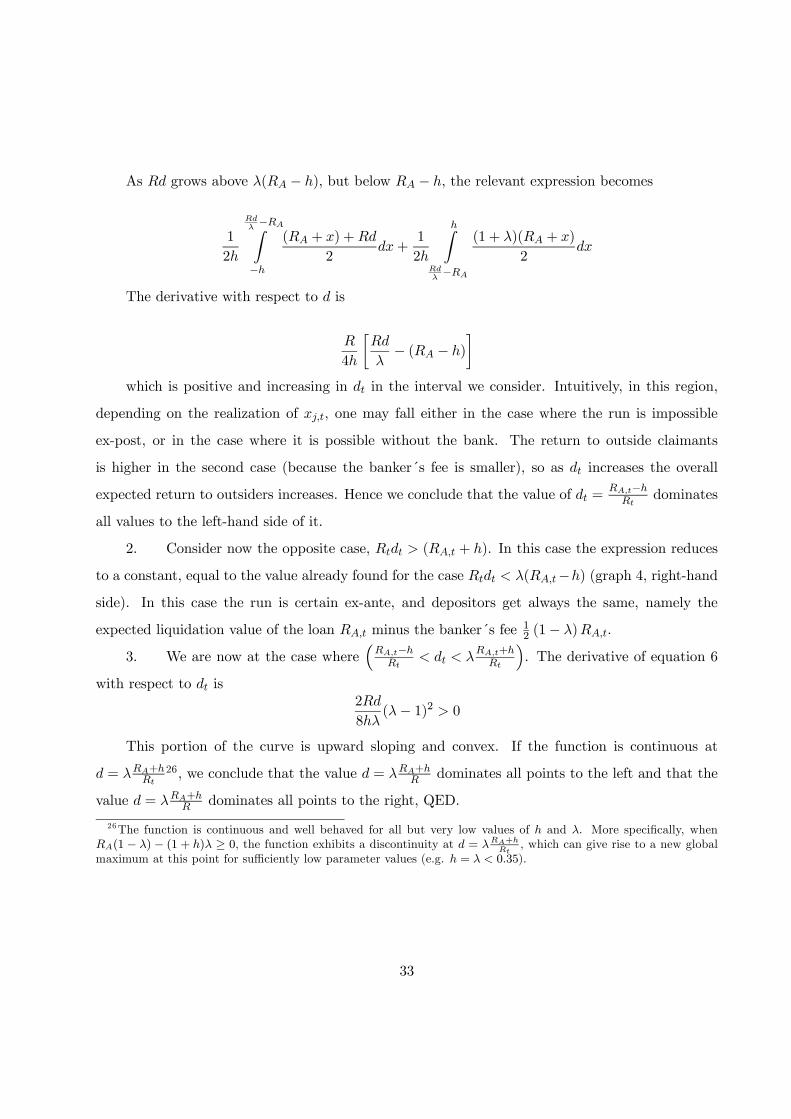
As grows above ( − ), but below − , the relevant expression becomes

1

2

−Z

−

( + ) +

2+

1

2

Z−

(1 + )( + )

2

The derivative with respect to is

4

∙

− ( − )

¸which is positive and increasing in in the interval we consider. Intuitively, in this region,

depending on the realization of , one may fall either in the case where the run is impossible

ex-post, or in the case where it is possible without the bank. The return to outside claimants

is higher in the second case (because the banker´s fee is smaller), so as increases the overall

expected return to outsiders increases. Hence we conclude that the value of =−

dominates

all values to the left-hand side of it.

2. Consider now the opposite case, ( + ). In this case the expression reduces

to a constant, equal to the value already found for the case (−) (graph 4, right-handside). In this case the run is certain ex-ante, and depositors get always the same, namely the

expected liquidation value of the loan minus the banker´s fee12(1− ).

3. We are now at the case where³−

+

´. The derivative of equation 6

with respect to is

2

8(− 1)2 0

This portion of the curve is upward sloping and convex. If the function is continuous at

= +

26, we conclude that the value = +

dominates all points to the left and that the

value = +

dominates all points to the right, QED.

26The function is continuous and well behaved for all but very low values of and . More specifically, when

(1 − ) − (1 + ) ≥ 0, the function exhibits a discontinuity at = +

, which can give rise to a new global

maximum at this point for sufficiently low parameter values (e.g. = 035).

33

10.1 Sensitivity to the density function: the case of normal distribution

Let us assume that follows a zero-mean normal distribution. The expected value of returns to

outside investors is

(1√22

)

⎧⎪⎪⎪⎪⎪⎪⎪⎪⎨⎪⎪⎪⎪⎪⎪⎪⎪⎩

−Z−∞

exph− 2

22

i(1+)(+)

2+

−Z

−

exph− 2

22

i(+)+

2+

∞Z−

exph− 2

22

i(1+)(+)

2

⎫⎪⎪⎪⎪⎪⎪⎪⎪⎬⎪⎪⎪⎪⎪⎪⎪⎪⎭Graph 5 shows the expected value of returns to outside investors for ranging between 0 and

1 under the following parameter set: = 103; = 101; = 05, when the distribution of

returns follows a standard normal ( = 03). Sensitivity analysis shows that, as with the uniform

distribution, the optimal value of is positively related to , and , and negatively related to

.

dopt 1d

Return to investors

Graph 5

34

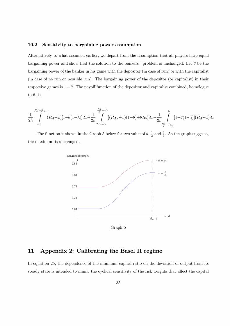
10.2 Sensitivity to bargaining power assumption

Alternatively to what assumed earlier, we depart from the assumption that all players have equal

bargaining power and show that the solution to the bankers ’ problem is unchanged. Let be the

bargaining power of the banker in his game with the depositor (in case of run) or with the capitalist

(in case of no run or possible run). The bargaining power of the depositor (or capitalist) in their

respective games is 1− . The payoff function of the depositor and capitalist combined, homologue

to 6, is

1

2

−Z−

(+)[1−(1−)]+ 1

2

−Z

−

[(+)(1−)+]+ 1

2

Z−

[1−(1−)](+)

The function is shown in the Graph 5 below for two value of , 12and 2

3. As the graph suggests,

the maximum is unchanged.

Θ 12

Θ 23

dopt 1d

0.65

0.70

0.75

0.80

0.85

Return to investors

Graph 5

11 Appendix 2: Calibrating the Basel II regime

In equation 25, the dependence of the minimum capital ratio on the deviation of output from its

steady state is intended to mimic the cyclical sensitivity of the risk weights that affect the capital

35

requirements under the Basel II Internal Ratings Based approach. The parameters 0 and 1 can

be calibrated so as to ensure that the resulting required capital ratio is, at each point in the cycle,

close to that resulting from the application of the actual Basel II IRB rules.

The IRB risk-weighted approach requires banks to hold capital to cover unexpected losses,

for a given confidence level, given the distribution of potential losses. Potential loan losses are

determined by the probability of default (PDs) of borrowers, which differ across rating classes, and

by their losses conditional on default (losses given default, or LGDs). This methodology, based

Merton [48], implies that the capital requirement for a unit of exposure is given by (for details see

Basel Committee on Banking Supervision [8])

=

½Φ

∙1√1−

Φ−1() +r

1−

¸Φ−1(999)−

¾

where is an estimate of the cross-borrower correlation and is an adjustment for average

loan maturity. The correlation is approximated by the Basel Committee by means of the following

function of PD:

= 012

∙1− exp(−50)1− exp(−50)

¸+ 024

∙1− 1− exp(−50)

1− exp(−50)¸

The maturity adjustment formula is given by

=1 + ( − 25)()

1− 15()where is the average maturity of loans, that we assume fixed and equal to 3 years.

We follow Darracq Paries et al. [23] in assuming that LGD is constant over the cycle and

equal to 0.45. On the contrary, PDs are typically found to be anticyclical — the stronger the

cyclical position, the lower the average PD of non-financial corporations. We modelled the link

between the aggregate PD and the cycle, for the euro area, with the following regression equation:

= + −1 − ∆( − ) + (1)

The equation has been estimated using quarterly euro area data; see table A1. is a

quarterly average of the median default probability of euro area non financial firms (source: Moody’s

KMV). depends on its own lagged value and the (change of) the ratio of output to its trend;

36

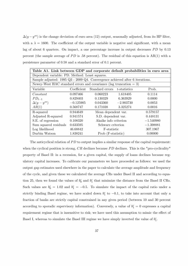
∆(− ) is the change deviation of euro area (12) output, seasonally adjusted, from its HP filter,

with a = 1600. The coefficient of the output variable is negative and significant, with a mean

lag of about 6 quarters. On impact, a one percentage increase in output decreases by 0.13

percent (the sample average of is .58 percent). The residual of this equation is AR(1) with a

persistence parameter of 0.58 and a standard error of 0.1 percent.

Table A1. Link between GDP and corporate default probabilities in euro area

Dependent variable: PD. Method: Least squares.

Sample adjusted: 1995 Q3 - 2009 Q4. Convergence achieved after 6 iterations.

Newey-West HAC standard errors and covariance (lag truncation = 3)

Variable Coefficient Standard errors t-statistics Prob.

0097466 0060223 1618405 01114

−1 0829403 0130329 6363929 00000

∆( − ) −0125905 0043360 −2903730 00053

(1) 0568747 0171038 3325274 00016

R-squared 0944649 Mean dependent var. 0579157

Adjusted R-squared 0941574 S.D. dependent var. 0448131

S.E. of regression 0108320 Akaike info criterion −1540980Sum squared residuals 0633595 Schwarz criterion −1398881Log likelihood 4668842 F-statistic 3071967

Durbin Watson 1838241 Prob (F-statistic) 000000

The anticyclical relation of to output implies a similar response of the capital requirement:

when the cyclical position is strong, declines because declines. This is the "pro-cyclicality"

property of Basel II: in a recession, for a given capital, the supply of loans declines because reg-

ulatory capital increases. To calibrate our parameters we have proceeded as follows: we used the

output gap estimates used elsewhere in the paper to calculate the average amplitude and frequency

of the cycle, and given these we calculated the average CRs under Basel II and according to equa-

tion 25, then we found the values of 0 and 1 that minimize the distance from the Basel II CRs.

Such values are 0 = 102 and 1 = −05. To simulate the impact of the capital ratio under astrictly binding Basel regime, we have scaled down 1 to −01, to take into account that only afraction of banks are strictly capital constrained in any given period (between 10 and 30 percent

according to sporadic supervisory information). Conversely, a value of 1 = 0 expresses a capital

requirement regime that is insensitive to risk; we have used this assumption to mimic the effect of

Basel I, whereas to simulate the Basel III regime we have simply inverted the value of 1.

37

References

[1] Acharya, Viral and Hassan Naqvi, 2010. “The Seeds of a Crisis: A Theory of Bank Liquidity

and Risk Taking over the Business Cycle.”

[2] Allen, Franklin, and Douglas Gale, 1994. “Liquidity Preferences, Market Participation and

asset Price Volatility”. American Economic Review, 84, 933-955.

[3] Allen, Franklin, and Douglas Gale, 2000. “Financial Contagion”. Journal of Political Economy,

108, 1-33.

[4] Allen, Franklin, and Douglas Gale, 2004. “Financial Intermediaries and Markets.” Economet-

rica, vol. 72(4), pages 1023-1061, 07.

[5] Altunbas Y., L. Gambacorta and D. Marques-Ibanez, 2009. “An Empirical Assessment of the

Risk-Taking Channel.” BIS, mimeo.

[6] Angeloni, Ignazio, Ester Faia and Marco Lo Duca, 2010. “Monetary Policy and Risk Taking”.

Mimeo.

[7] Bernanke, Ben and Mark Gertler, 1999. “Monetary policy and asset price volatility.” Proceed-

ings, Federal Reserve Bank of Kansas City, pages 77-12.

[8] An explanatory note on the Basel II IRB risk-weights functions, July 2005, available at

http://www.bis.org/bcbs/index.htm

[9] Bernanke, B., M. Gertler and S. Gilchrist, 1999. “The Financial Accelerator in a Quantitative

Business Cycle Framework”. in J.B. Taylor, and M. Woodford, eds., Handbook of Macroeco-

nomics, Amsterdam: North-Holland.

[10] Bils M. and P. Klenow 2004. “Some Evidence on the Importance of Sticky Prices”. Journal of

Political Economy, October.

[11] Bloom, Nicholas 2008. “The Impact of Uncertainty Shocks.” Forthcoming in Econometrica.

[12] Bloom, Nicholas, Max Floteotto and Nir Jiaimovich, 2009. “Really Uncertain Business Cycles”.

Mimeo.

38

[13] Blum, J. and M. Hellwig, 1995. “The Macroeconomic Implications of Capital Requirements

Adequacy for Banks”. European Economic Review, vol. 39.

[14] Borio, Claudio, 2008. “The Macro-prudential Approach to Regulation and Supervision: Where

Do We Stand?”. in D. Mayes, R. Pringle and M. Taylor (eds), New Frontier in Regulation and

Official Oversight of the Financial System, Central Banking Publications, forthcoming.

[15] Borio, Claudio and H. Zhu 2008. “Capital regulation, risk-taking and monetary policy: a

missing link in the transmission mechanism?” BIS Working Papers No. 268.

[16] Brunnermeier, M., A, Crockett, C. Goodhart, M. Hellwig, A. Persaud and H. Shin, 2009. “The

Fundamental Principles of Financial Regulation”. Geneva Report on the World Economy 11,

CEPR and ICMB.

[17] Brunnermeier, Markus, and Yuliy Sannikov, 2010. “A Macroeconomic Model with a Financial

Sector”. Mimeo. Princeton University.

[18] Checchetti, Stephen and Li Lianfa, 2008. “Do Capital Adequacy Requirements Matter for

Monetary Policy?”. Economic Inquiry, 46(4).

[19] Carlstrom, Charles T & Fuerst, Timothy S, 1997. “Agency Costs, Net Worth, and Business

Fluctuations: A Computable General Equilibrium Analysis.” American Economic Review, vol.

87(5), pages 893-910.

[20] Cecchetti, S.G., H. Genberg, J. Lipsky and S. Whadwani, 2000. “Asset Prices and Central

Bank Policy”. Geneva Report on the World Economy 2, CEPR and ICMB.

[21] Christiano, L., R. Motto and M. Rostagno 2007. “Financial Factors in Business Cycles”.

mimeo.

[22] Covas, F. and S. Fujita, 2009. “Time-varying capital requirements in a general equilibrium

model of liquidity dependence”. Philadelphia Fed Working paper 09-23.

[23] Darracq Pariès, Matthieu, Christoffer Kok Sørensen and Diego Rodriguez Palenzuela, 2010.

“Macroeconomic propagation under different regulatory regimes”. ECB Mimeo.

39

[24] Corbae, Dean and Pablo, D’Erasmo, 2010. “A Quantitative Model of Banking Industry Dy-

namics”.

[25] Diamond, Douglas W., 1984. “Financial Intermediation and Delegated Monitoring.” Review

of Economic Studies.

[26] Diamond, Douglas W. and P. Dybvig, 1983. “Bank Runs, Liquidity, and Deposit Insurance”.

Journal of Political Economy, 91, 401-419.

[27] Diamond, Douglas W. and Rajan, Raghuram G. 2000. “A Theory of Bank Capital”. Journal

of Finance, vol. LV. No. 6.

[28] Douglas W. Diamond and Raghuram G. Rajan, 2006. “Money in a Theory of Banking.”

American Economic Review, vol. 96(1), pages 30-53.

[29] Douglas, Diamond W. and Raghuram G. Rajan, 2001. “Liquidity Risk, Liquidity Creation and

Financial Fragility: A Theory of Banking.” Journal of Political Economy.

[30] Faia, Ester, 2008. “Optimal Monetary Policy Rules with Labor Market Frictions”. Journal of

Economic Dynamics and Control.

[31] Faia, Ester, 2009. “Ramsey Monetary Policy with Labour Market Frictions”. Journal of Mon-

etary Economics, Vol. 56:4.

[32] Faia, Ester, 2010. “Credit Risk Transfers and the Macroeconomy”. Mimeo.

[33] Faia, Ester, Monacelli, Tommaso, 2007. “Optimal interest rate rules, asset prices, and credit

frictions”. Journal of Economic Dynamics and Control.

[34] Galí, J. and M. Gertler 1999. “Inflation Dynamics: A Structural Econometric Analysis”. Jour-

nal of Monetary Economics, vol. 44, n 2, 195-222.

[35] Gertler, Mark and Peter Karadi, 2009. “A Model of Unconventional Monetary Policy”. NYU.

[36] Gertler, Mark and Nobuhiro Kiyotaki, 2009. “Financial Intermediation and Credit Policy in

Business Cycle Analysis”. mimeo.

40

[37] He, Zhiguo, and Arvind Krishnamurthy, 2009. “A Model of Capital and Crises”. Mimeo,

University of Chicago.

[38] Holmstrom, Bengt and Tirole, Jean, 1997. “Financial Intermediation, Loanable Funds, and

the Real Sector.” The Quarterly Journal of Economics, MIT Press, vol. 112(3), pages 663-91.

[39] Iacoviello, Matteo, 2005. “House Prices, Borrowing Constraints and Monetary Policy in the

Business Cycle.” American Economic Review, Vol. 95, No. 3, pp. 739-764.

[40] Iacoviello, Matteo, 2010. “Financial Business Cycles.” Mimeo.

[41] Kashyap, Anil and Jeremy Stein, 2004. “Cyclical Implications of the Basel II Capital Stan-

dards”. Economic Perspectives, The Federal Reserve Bank of Chicago.

[42] Kim, Jinill and Sunghyun Henry Kim, 2003. “Spurious Welfare Reversals in International

Business Cycles”. Journal of International Economics, 60, p. 471-500.

[43] King R. and S. Rebelo, 1999. “Resuscitating Real Business Cycles”. in J.B. Taylor, and M.

Woodford, eds., Handbook of Macroeconomics, Amsterdam: North-Holland.

[44] Kiyotaki, Nobuhiro and Moore, John 1997. “Credit Cycles”. Journal of Political Economy 105

(2): 211—248.

[45] Lorenzoni, Guido, 2008. “Inefficient Credit Booms”. Review of Economic Studies, 75 (3), 809-

833

[46] Maddaloni A., and J.L. Peydró Alcalde, 2009. “Bank risk-taking, Securitization and Monetary

Policy; Evidence from the bank Lending Survey”. ECB, mimeo.

[47] Meh. C.A., and K. Moran, 2008. “The role of bank capital in the propagation of shocks”.

Journal of Economic Dynamics and Control, 2008

[48] Merton, R. C., 1974. “On the pricing of corporate debt: The risk structure of interest rates”.

Journal of Finance 29, 449 - 470.

[49] Morris, S. and H.S. Shin, 2008. “Financial Regulation in a System Context”. Brookings Papers

of Economic Activity.

41

[50] Perotti, R. 2004. “Estimating the Effects of Fiscal Policy in OECD Countries”. Mimeo IGIER

Bocconi.

[51] Elizaldea, A and R. Repullo, 2007. “Economic and Regulatory Capital in Banking: What Is

the Difference?”. International Journal of Central Banking 3, pp. 87-117.

[52] Rudebusch, Glenn D., 2002. “Term structure evidence on interest rate smoothing and monetary

policy inertia.” Journal of Monetary Economics, vol. 49(6), pages 1161-1187, September.

[53] Sbordone A. (2002). “Prices and Unit Labor Costs: A New Test of Price Stickiness”. Journal

of Monetary Economics Vol. 49 (2).

[54] Schmitt-Grohe S. and M. Uribe, 2003. “Optimal, Simple and Implementable Monetary and

Fiscal Rules.” Mimeo Duke University.

[55] Schmitt-Grohe, Stephanie and Uribe, Martin, 2004a. “Solving Dynamic General Equilibrium

Models Using a Second-Order Approximation to the Policy Function.” Journal of Economic

Dynamics and Control 28, 645-858.

[56] Schmitt-Grohe S. and M. Uribe, 2004b. “Optimal Operational Monetary Policy in Christiano-

Eichenbaum-Evans Model of the U.S. Business Cycle.” Mimeo Duke University.

[57] Woodford, Michael, 2003. Interest and Prices.

42

Graph 1: Bank capital structure and the risk of bank run

X -h h

A B C D

x

RA

λ(RA+x)

43

0 5 10 15 20 25 30 35 40-0.4

-0.3

-0.2

-0.1

0Inflation

0 5 10 15 20 25 30 35 400

0.5

1

1.5Output

0 5 10 15 20 25 30 35 40-0.2

0

0.2

0.4

0.6Employment

0 5 10 15 20 25 30 35 40-0.5

-0.4

-0.3

-0.2

-0.1

0Interest rate

0 5 10 15 20 25 30 35 40-0.1

0

0.1

0.2

0.3Tobin Q

0 5 10 15 20 25 30 35 40-2

0

2

4

6Investment

0 5 10 15 20 25 30 35 400

0.1

0.2

0.3

0.4Capital

0 5 10 15 20 25 30 35 40-0.4

-0.3

-0.2

-0.1

0Bank ROA

0 5 10 15 20 25 30 35 400

0.05

0.1

0.15

0.2Deposit ratio

0 5 10 15 20 25 30 35 400.05

0.1

0.15

0.2

0.25

0.3Bank riskiness

Figure 1: Impulse response to a positive productivity shock

44

0 5 10 15 20 25 30 35 40-0.15

-0.1

-0.05

0

0.05Inflation

0 5 10 15 20 25 30 35 40-2

-1.5

-1

-0.5

0

0.5Output

0 5 10 15 20 25 30 35 40-3

-2

-1

0

1Employment

0 5 10 15 20 25 30 35 400

0.2

0.4

0.6

0.8Interest rate

0 5 10 15 20 25 30 35 40-0.6

-0.4

-0.2

0

0.2Tobin Q

0 5 10 15 20 25 30 35 40-15

-10

-5

0

5Investment

0 5 10 15 20 25 30 35 40-0.4

-0.3

-0.2

-0.1

0Capital

0 5 10 15 20 25 30 35 400

0.2

0.4

0.6

0.8

1Bank ROA

0 5 10 15 20 25 30 35 40-0.08

-0.06

-0.04

-0.02

0Deposit ratio

0 5 10 15 20 25 30 35 40-0.8

-0.6

-0.4

-0.2

0Bank riskiness

Figure 2: Impulse response to a positive interest rate shock

45

0 5 10 15 20 25 30 35 40-15

-10

-5

0

5x 10

-3Inflation

0 5 10 15 20 25 30 35 40-0.1

0

0.1

0.2

0.3

0.4Output

0 5 10 15 20 25 30 35 40-0.2

0

0.2

0.4

0.6Employment

0 5 10 15 20 25 30 35 40-0.02

0

0.02

0.04Interest rate

0 5 10 15 20 25 30 35 40-0.05

0

0.05

0.1

0.15Tobin Q

0 5 10 15 20 25 30 35 40-1

0

1

2

3Investment

0 5 10 15 20 25 30 35 400

0.02

0.04

0.06

0.08Capital

0 5 10 15 20 25 30 35 40-0.05

0

0.05

0.1

0.15Bank ROA

0 5 10 15 20 25 30 35 400

0.01

0.02

0.03

0.04Deposit ratio

0 5 10 15 20 25 30 35 40-0.15

-0.1

-0.05

0

0.05Bank riskiness

Figure 3: Impulse response to a positive shock in the marginal return on capital

46

0 5 10 15 20 25 30 35 40-0.4

-0.3

-0.2

-0.1

0Inflation

0 5 10 15 20 25 30 35 400

0.5

1

1.5Output

0 5 10 15 20 25 30 35 40-0.2

0

0.2

0.4

0.6Employment

0 5 10 15 20 25 30 35 40-0.5

-0.4

-0.3

-0.2

-0.1

0Interest rate

0 5 10 15 20 25 30 35 40-0.1

0

0.1

0.2

0.3Tobin Q

0 5 10 15 20 25 30 35 40-1

0

1

2

3

4

5Investment

0 5 10 15 20 25 30 35 400

0.1

0.2

0.3

0.4

0.5Capital

0 5 10 15 20 25 30 35 40-0.4

-0.3

-0.2

-0.1

0Bank ROA

0 5 10 15 20 25 30 35 400

0.05

0.1

0.15

0.2Deposit ratio

0 5 10 15 20 25 30 35 400.05

0.1

0.15

0.2

0.25

0.3Bank riskiness

lambda=0.45

lambda=0.65

Figure 4: Alternative values of lambda (positive productivity shock)

47

0 5 10 15 20 25 30 35 40-0.4

-0.3

-0.2

-0.1

0Inflation

0 5 10 15 20 25 30 35 400

0.5

1

1.5Output

0 5 10 15 20 25 30 35 40-0.2

0

0.2

0.4

0.6Employment

0 5 10 15 20 25 30 35 40-0.5

-0.4

-0.3

-0.2

-0.1

0Interest rate

0 5 10 15 20 25 30 35 40-0.1

0

0.1

0.2

0.3Tobin Q

0 5 10 15 20 25 30 35 40-1

0

1

2

3

4

5Investment

0 5 10 15 20 25 30 35 400

0.1

0.2

0.3

0.4Capital

0 5 10 15 20 25 30 35 40-0.4

-0.3

-0.2

-0.1

0Bank ROA

0 5 10 15 20 25 30 35 400

0.05

0.1

0.15

0.2

0.25Deposit ratio

0 5 10 15 20 25 30 35 400.05

0.1

0.15

0.2

0.25

0.3Bank riskiness

h=0.45

h=0.65

Figure 5: Alternative values of h (positive productivity shock)

48

0 5 10 15 20 25 30 35 40-0.15

-0.1

-0.05

0

0.05

0.1Inflation

0 5 10 15 20 25 30 35 40-2.5

-2

-1.5

-1

-0.5

0

0.5Output

0 5 10 15 20 25 30 35 40-4

-3

-2

-1

0

1Employment

0 5 10 15 20 25 30 35 400

0.2

0.4

0.6

0.8Interest rate

0 5 10 15 20 25 30 35 40-0.8

-0.6

-0.4

-0.2

0

0.2Tobin Q

0 5 10 15 20 25 30 35 40-15

-10

-5

0

5Investment

0 5 10 15 20 25 30 35 40-0.5

-0.4

-0.3

-0.2

-0.1

0Capital

0 5 10 15 20 25 30 35 400

0.5

1

1.5Bank ROA

0 5 10 15 20 25 30 35 40-0.1

-0.08

-0.06

-0.04

-0.02

0Deposit ratio

0 5 10 15 20 25 30 35 40-0.8

-0.6

-0.4

-0.2

0Bank riskiness

h=0.45

h=0.65

Figure 6: Alternative values of h (positive interest rate shock)

49

0 5 10 15 20 25 30 35 40-0.015

-0.01

-0.005

0

0.005

0.01Inflation

0 5 10 15 20 25 30 35 40-0.1

0

0.1

0.2

0.3

0.4Output

0 5 10 15 20 25 30 35 40-0.2

0

0.2

0.4

0.6Employment

0 5 10 15 20 25 30 35 40-0.02

0

0.02

0.04

0.06

0.08Interest rate

0 5 10 15 20 25 30 35 40-0.05

0

0.05

0.1

0.15Tobin Q

0 5 10 15 20 25 30 35 40-1

0

1

2

3Investment

0 5 10 15 20 25 30 35 400

0.02

0.04

0.06

0.08Capital

0 5 10 15 20 25 30 35 40-0.05

0

0.05

0.1

0.15

0.2Bank ROA

0 5 10 15 20 25 30 35 400

0.01

0.02

0.03

0.04Deposit ratio

0 5 10 15 20 25 30 35 40-0.2

-0.15

-0.1

-0.05

0

0.05Bank riskiness

Standard Taylor

Response to asset price

Response to bank leverage

Figure 7: Response to asset prices or leverage (positive shock on marginal return on capital)

50

0 5 10 15 20 25 30 35 40-0.5

-0.4

-0.3

-0.2

-0.1

0Inflation

0 5 10 15 20 25 30 35 400

0.5

1

1.5

2

2.5

3Output

0 5 10 15 20 25 30 35 40-1

0

1

2

3Employment

0 5 10 15 20 25 30 35 40-0.8

-0.6

-0.4

-0.2

0Interest rate

0 5 10 15 20 25 30 35 40-0.5

0

0.5

1Tobin Q

0 5 10 15 20 25 30 35 40-5

0

5

10

15

20Investment

0 5 10 15 20 25 30 35 40-0.5

0

0.5

1

1.5Capital

0 5 10 15 20 25 30 35 40-0.8

-0.6

-0.4

-0.2

0Bank ROA

0 5 10 15 20 25 30 35 400

0.1

0.2

0.3

0.4Deposit ratio

0 5 10 15 20 25 30 35 40-0.5

0

0.5

1

1.5

2Bank riskiness

Basel I

Basel II

Basel III

Figure 8: Comparing Basel regimes with soft-binding constraint (positive productivity shocks)

51

0 5 10 15 20 25 30 35 40-0.4

-0.3

-0.2

-0.1

0Inflation

0 5 10 15 20 25 30 35 400

0.5

1

1.5

2Output

0 5 10 15 20 25 30 35 40-1

-0.5

0

0.5

1

1.5Employment

0 5 10 15 20 25 30 35 40-0.8

-0.6

-0.4

-0.2

0Interest rate

0 5 10 15 20 25 30 35 40-0.2

0

0.2

0.4

0.6Tobin Q

0 5 10 15 20 25 30 35 40-5

0

5

10Investment

0 5 10 15 20 25 30 35 40-0.2

0

0.2

0.4

0.6

0.8Capital

0 5 10 15 20 25 30 35 40-0.6

-0.4

-0.2

0

0.2Bank ROA

0 5 10 15 20 25 30 35 40-2

-1

0

1

2Deposit ratio

0 5 10 15 20 25 30 35 40-0.4

-0.2

0

0.2

0.4

0.6Bank riskiness

Basel I

Basel II

Basel III

Figure 9: Comparing Basel regimes with hard-binding constraint (positive productivity shocks)

52

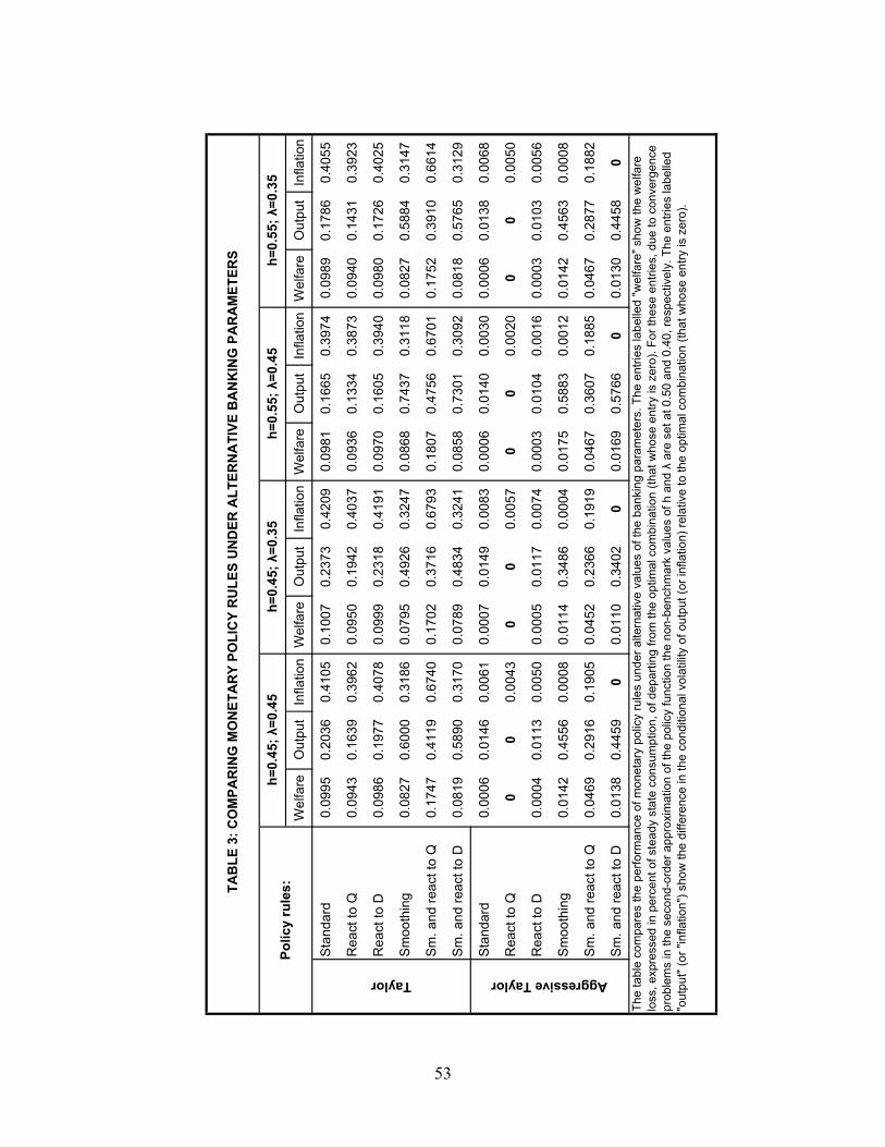
Wel

fare

Out

put

Infla

tion

Wel

fare

Out

put

Infla

tion

Wel

fare

Out

put

Infla

tion

Wel

fare

Out

put

Infla

tion

Sta

ndar

d 0.

0995

0.20

360.

4105

0.10

070.

2373

0.42

090.

0981

0.16

650.

3974

0.09

890.

1786

0.40

55

Rea

ct to

Q0.

0943

0.16

390.

3962

0.09

500.

1942

0.40

370.

0936

0.13

340.

3873

0.09

400.

1431

0.39

23

Rea

ct to

D0.

0986

0.19

770.

4078

0.09

990.

2318

0.41

910.

0970

0.16

050.

3940

0.09

800.

1726

0.40

25

Sm

ooth

ing

0.08

270.

6000

0.31

860.

0795

0.49

260.

3247

0.08

680.

7437

0.31

180.

0827

0.58

840.

3147

Sm

. and

reac

t to

Q0.

1747

0.41

190.

6740

0.17

020.

3716

0.67

930.

1807

0.47

560.

6701

0.17

520.

3910

0.66

14

Sm

. and

reac

t to

D0.

0819

0.58

900.

3170

0.07

890.

4834

0.32

410.

0858

0.73

010.

3092

0.08

180.

5765

0.31

29

Sta

ndar

d 0.

0006

0.01

460.

0061

0.00

070.

0149

0.00

830.

0006

0.01

400.

0030

0.00

060.

0138

0.00

68

Rea

ct to

Q0

00.

0043

00

0.00

570

00.

0020

00

0.00

50

Rea

ct to

D0.

0004

0.01

130.

0050

0.00

050.

0117

0.00

740.

0003

0.01

040.

0016

0.00

030.

0103

0.00

56

Sm

ooth

ing

0.01

420.

4556

0.00

080.

0114

0.34

860.

0004

0.01

750.

5883

0.00

120.

0142

0.45

630.

0008

Sm

. and

reac

t to

Q0.

0469

0.29

160.

1905

0.04

520.

2366

0.19

190.

0467

0.36

070.

1885

0.04

670.

2877

0.18

82

Sm

. and

reac

t to

D0.

0138

0.44

590

0.01

100.

3402

00.

0169

0.57

660

0.01

300.

4458

0Th

e ta

ble

com

pare

s th

e pe

rform

ance

of m

onet

ary

polic

y ru

les

unde

r alte

rnat

ive

valu

es o

f the

ban

king

par

amet

ers.

The

ent

ries

labe

lled

"wel

fare

" sho

w th

e w

elfa

re

loss

, exp

ress

ed in

per

cent

of s

tead

y st

ate

cons

umpt

ion,

of d

epar

ting

from

the

optim

al c

ombi

natio

n (th

at w

hose

ent

ry is

zer

o). F

or th

ese

entri

es, d

ue to

con

verg

ence

pr

oble

ms

in th

e se

cond

-ord

er a

ppro

xim

atio

n of

the

polic

y fu

nctio

n th

e no

n-be

nchm

ark

valu

es o

f h a

nd λ

are

set

at 0

.50

and

0.40

, res

pect

ivel

y. T

he e

ntrie

s la

belle

d "o

utpu

t" (o

r "in

flatio

n") s

how

the

diffe

renc

e in

the

cond

ition

al v

olat

ility

of o

utpu

t (or

infla

tion)

rela

tive

to th

e op

timal

com

bina

tion

(that

who

se e

ntry

is z

ero)

.

Polic

y ru

les:TA

BLE

3: C

OM

PAR

ING

MO

NET

AR

Y PO

LIC

Y R

ULE

S U

ND

ER A

LTER

NA

TIVE

BA

NK

ING

PA

RA

MET

ERS

Taylor Aggressive Taylor

h=0.

45; λ

=0.4

5h=

0.45

; λ=0

.35

h=0.

55; λ

=0.4

5h=

0.55

; λ=0

.35

53

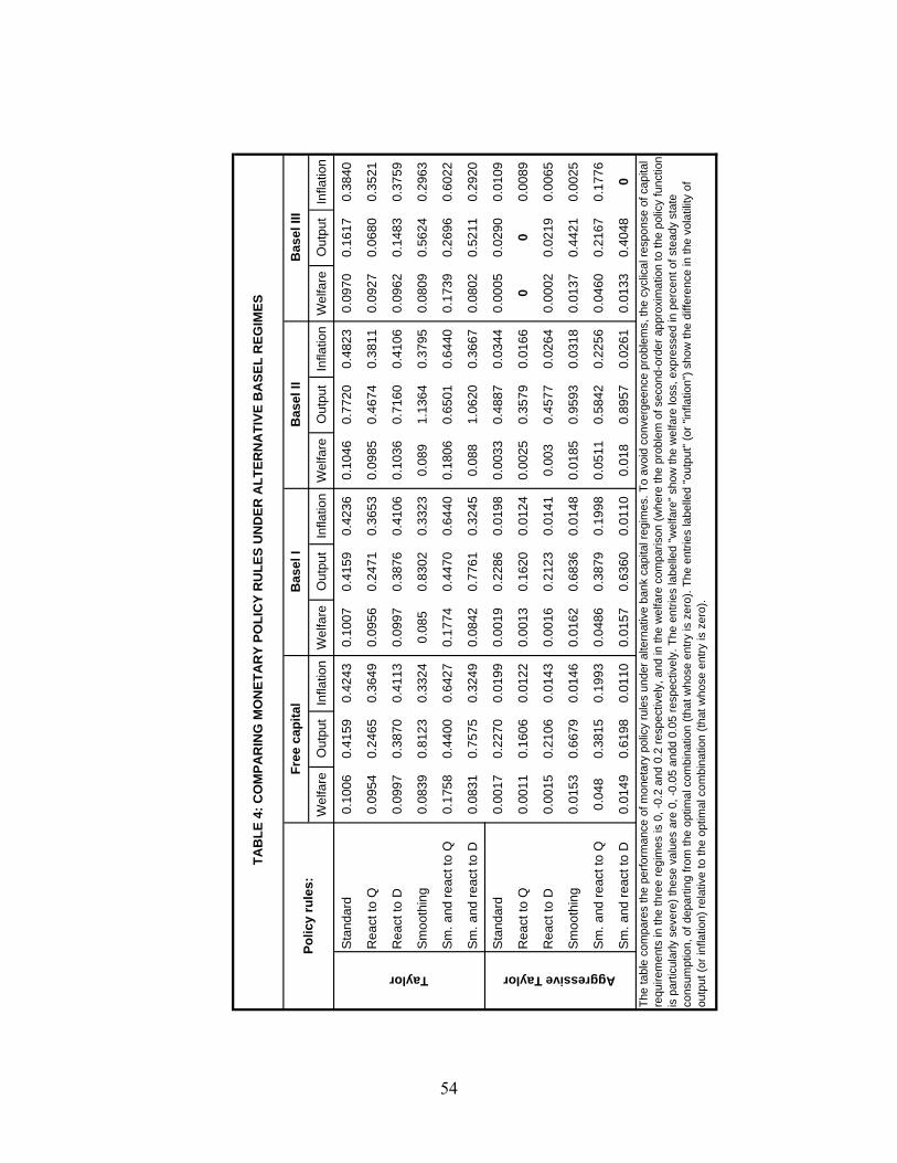
Wel

fare

Out

put

Infla

tion

Wel

fare

Out

put

Infla

tion

Wel

fare

Out

put

Infla

tion

Wel

fare

Out

put

Infla

tion

Sta

ndar

d 0.

1006

0.41

590.

4243

0.10

070.

4159

0.42

360.

1046

0.77

200.

4823

0.09

700.

1617

0.38

40

Rea

ct to

Q0.

0954

0.24

650.

3649

0.09

560.

2471

0.36

530.

0985

0.46

740.

3811

0.09

270.

0680

0.35

21

Rea

ct to

D0.

0997

0.38

700.

4113

0.09

970.

3876

0.41

060.

1036

0.71

600.

4106

0.09

620.

1483

0.37

59

Sm

ooth

ing

0.08

390.

8123

0.33

240.

085

0.83

020.

3323

0.08

91.

1364

0.37

950.

0809

0.56

240.

2963

Sm

. and

rea

ct to

Q0.

1758

0.44

000.

6427

0.17

740.

4470

0.64

400.

1806

0.65

010.

6440

0.17

390.

2696

0.60

22

Sm

. and

rea

ct to

D0.

0831

0.75

750.

3249

0.08

420.

7761

0.32

450.

088

1.06

200.

3667

0.08

020.

5211

0.29

20

Sta

ndar

d 0.

0017

0.22

700.

0199

0.00

190.

2286

0.01

980.

0033

0.48

870.

0344

0.00

050.

0290

0.01

09

Rea

ct to

Q0.

0011

0.16

060.

0122

0.00

130.

1620

0.01

240.

0025

0.35

790.

0166

00

0.00

89

Rea

ct to

D0.

0015

0.21

060.

0143

0.00

160.

2123

0.01

410.

003

0.45

770.

0264

0.00

020.

0219

0.00

65

Sm

ooth

ing

0.01

530.

6679

0.01

460.

0162

0.68

360.

0148

0.01

850.

9593

0.03

180.

0137

0.44

210.

0025

Sm

. and

rea

ct to

Q0.

048

0.38

150.

1993

0.04

860.

3879

0.19

980.

0511

0.58

420.

2256

0.04

600.

2167

0.17

76

Sm

. and

rea

ct to

D0.

0149

0.61

980.

0110

0.01

570.

6360

0.01

100.

018

0.89

570.

0261

0.01

330.

4048

0T

he ta

ble

com

pare

s th

e pe

rfor

man

ce o

f mon

etar

y po

licy

rule

s un

der

alte

rnat

ive

bank

cap

ital r

egim

es. T

o av

oid

conv

erge

ence

pro

blem

s, th

e cy

clic

al r

espo

nse

of c

apita

l re

quire

men

ts in

the

thre

e re

gim

es is

0, -

0.2

and

0.2

resp

ectiv

ely,

and

in th

e w

elfa

re c

ompa

rison

(w

here

the

prob

lem

of s

econ

d-o

rder

app

roxi

mat

ion

to th

e po

licy

func

tion

is p

artic

ular

ly s

ever

e) th

ese

valu

es a

re 0

, -0.

05 a

ndd

0.05

res

pect

ivel

y. T

he e

ntrie

s la

belle

d "w

elfa

re"

show

the

wel

fare

loss

, ex

pres

sed

in p

erce

nt o

f ste

ady

stat

e co

nsum

ptio

n, o

f dep

artin

g fr

om th

e op

timal

com

bina

tion

(tha

t who

se e

ntry

is z

ero)

. The

ent

ries

labe

lled

"out

put"

(or

"in

flatio

n")

sho

w th

e di

ffere

nce

in th

e vo

latil

ity o

f ou

tput

(or

infla

tion)

rel

ativ

e to

the

optim

al c

ombi

natio

n (t

hat w

hose

ent

ry is

zer

o).

Taylor Aggressive Taylor

TAB

LE 4

: CO

MPA

RIN

G M

ON

ETA

RY

POLI

CY

RU

LES

UN

DER

ALT

ERN

ATI

VE B

ASE

L R

EGIM

ES

Polic

y ru

les:

Free

cap

ital

Bas

el I

Bas

el II

Bas

el II

I

54

Wel

fare

Out

put

Infla

tion

Wel

fare

Out

put

Infla

tion

Wel

fare

Out

put

Infla

tion

Sta

ndar

d 0.

0614

0.80

140.

5574

0.06

751.

2661

0.60

770.

0583

0.52

960.

5428

Rea

ct to

Q0.

0594

0.79

110.

5453

0.06

481.

2456

0.58

570.

0569

0.52

440.

5361

Rea

ct to

D0.

0614

0.80

140.

5574

0.13

382.

3993

1.12

060.

0192

0.08

800.

1010

Sm

ooth

ing

0.06

861.

0557

0.55

080.

0844

2.17

320.

6724

0.06

190.

7068

0.52

52

Sm

. and

rea

ct to

Q0.

1400

1.58

890.

8308

0.17

293.

6066

0.96

620.

1265

1.07

110.

8008

Sm

. and

rea

ct to

D0.

0686

1.05

570.

5508

0.15

794.

6099

1.17

560.

0285

0.32

660.

1853

Sta

ndar

d 0.

0106

0.38

020.

2145

0.01

220.

7123

0.23

210.

0103

0.19

430.

2188

Rea

ct to

Q0.

0105

0.37

760.

2124

0.01

190.

7046

0.22

630.

0102

0.19

320.

2182

Rea

ct to

D0.

0106

0.38

020.

2145

0.03

051.

1474

0.49

120

00

Sm

ooth

ing

0.01

980.

5667

0.24

980.

0239

1.08

960.

2963

0.01

840.

3549

0.24

49

Sm

. and

rea

ct to

Q0.

0429

0.79

780.

3985

0.05

211.

6667

0.45

550.

0391

0.50

870.

3880

Sm

. and

rea

ct to

D0.

0198

0.56

670.

2498

0.04

562.

0547

0.55

640.

0088

0.17

880.

0838

Taylor Aggressive Taylor

The

tabl

e co

mpa

res

the

perf

orm

ance

of m

onet

ary

polic

y ru

les

unde

r al

tern

ativ

e ba

nk c

apita

l reg

imes

. The

cyc

lical

res

pons

e of

ca

pita

l req

uire

men

ts in

the

thre

e re

gim

es is

0, -

0.1

and

0.1

resp

ectiv

ely.

The

ent

ries

labe

lled

"wel

fare

" sh

ow th

e w

elfa

re lo

ss,

expr

esse

d in

per

cent

of s

tead

y st

ate

cons

umpt

ion,

of d

epar

ting

from

the

optim

al c

ombi

natio

n (t

hat w

hose

ent

ry is

zer

o). F

or th

ese

en

trie

s, d

ue to

con

verg

ence

pro

blem

s th

e cy

clic

al r

espo

nse

of c

apita

l req

uire

men

ts in

the

thre

e re

gim

es is

set

at 0

, -0.

05 a

nd 0

.05

resp

ectiv

ely

The

ent

ries

labe

lled

"out

put"

(or

"in

flatio

n")

show

the

diffe

renc

e in

the

vola

tility

of o

utpu

t (or

infla

tion)

rel

ativ

e to

the

optim

al c

ombi

natio

n (t

hat w

hose

ent

ry is

zer

o).

TAB

LE 5

: CO

MPA

RIN

G M

ON

ETA

RY

POLI

CY

RU

LES

UN

DER

ALT

ERN

ATI

VE B

ASE

L R

EGIM

ES

(with

str

ictly

bin

ding

cap

ital r

equi

rem

ent)

Polic

y ru

les:

Bas

el I

Bas

el II

Bas

el II

I

55