Capital Structure Decisions*

Murray Z. Frank

and

Vidhan K. Goyal

April 17, 2003

Abstract

This paper examines the relative importance of 39 factors in the leverage decisions of publicly traded U.S. firms. The pecking order and market timing theories do not provide good descriptions of the data. The evidence is generally consistent with tax/bankruptcy tradeoff theory and with stakeholder co-investment theory. The most reliable factors are median industry leverage (+ effect on leverage), bankruptcy risk as measured by Altman�s Z-Score (- effect on leverage), firm size as measured by the log of sales (+), dividend- paying (-), intangibles (+), market-to-book ratio (-), and collateral (+). Somewhat less reliable effects are the variance of own stock returns (-), net operating loss carry forwards (-), financially constrained (-), profitability (-), change in total corporate assets (+), the top corporate income tax rate (+), and the Treasury bill rate (+). Using Markov Chain Monte Carlo multiple imputation to correct for missing-data-bias we find that the effect of profits and net operating loss carry forwards are not robust. JEL classification: G32 Keywords: Capital structure, pecking order theory, tradeoff theory, stakeholder co-investment.

* The respective affiliations are: Murray Frank, Faculty of Commerce, University of British Columbia, Vancouver BC, Canada V6T 1Z2. Phone: 604-822-8480, Fax: 604-822-8477, E-mail: Murray.Frank@commerce.ubc.ca. Vidhan Goyal (corresponding author), Department of Finance, Hong Kong University of Science and Technology, Clear Water Bay, Kowloon, Hong Kong. Phone: +852 2358-7678, Fax: +852 2358-1749, E-mail: goyal@ust.hk. Thanks to Werner Antweiler and Kai Li for helpful comments. Murray Frank thanks the B.I. Ghert Family Foundation and the SSHRC for financial support. We are responsible for any errors. The appendix to this paper, along with many files that provide extra detail can be found at: http://www.bm.ust.hk/~vidhan/main.htm.

1

1. Introduction

What factors determine the capital structure decisions made by publicly traded U.S. firms?

Despite decades of intensive research, there is a surprising lack of consensus even about many of

the basic empirical facts. This is unfortunate for financial theory since disagreement over basic

facts implies disagreement about desirable features for theories. This is also unfortunate for

empirical research in corporate finance since it is unclear what factors should be used to control

for �what we already know.�

The survey by Harris and Raviv (1991) and the empirical study by Titman and Wessels

(1988) are commonly cited as sources for basic empirical facts about capital structure decisions.

These two classic papers illustrate the problem of disagreements over basic facts. According to

Harris and Raviv (1991, page 334), the available studies �generally agree that leverage increases

with fixed assets, non-debt tax shields, growth opportunities, and firm size and decreases with

volatility, advertising expenditures, research and development expenditures, bankruptcy

probability, profitability and uniqueness of the product.� However, Titman and Wessels (1988,

page 17) find that their �results do not provide support for an effect on debt ratios arising from

non-debt tax shields, volatility, collateral value, or future growth.� Consequently, different studies

employ different factors to control for what is �already known.�

This study contributes to our understanding of capital structure in four main ways. First, a

level playing field is created that includes 39 factors. This set of factors includes the major factors

considered in the literature. Much of the analysis is devoted to determining which factors are

reliably signed, and reliably important, for predicting leverage. Second, there is good reason to

suspect that patterns of corporate financing decisions may have changed over the decades. We

therefore examine whether such changes have taken place. Third, many firms have incomplete

records leading to the common practice of deleting firms for which some of the necessary data

items are missing. This can create missing-data-bias. We control for missing-data-bias through

the use of multiple imputation. Finally, it has been argued that different theories apply to firms

under different circumstances. �There is no universal theory of capital structure, and no reason to

expect one. There are useful conditional theories, however� Each factor could be dominant for

some firms or in some circumstances, yet unimportant elsewhere� (Myers (2002)). To address

this serious concern, the effect of conditioning on firm circumstances is studied.

We compare the evidence to predictions from the following theories. (1) The pecking order

2

theory: Due to adverse selection, firms prefer to finance their activities using retained earnings if

possible. If retained earnings are inadequate, then they turn to the use of debt. Equity financing is

only used as a last resort. (2) The market timing theory: Firms try to time the market by using

debt when it is cheap and equity when it seems cheap. (3) The tax/bankruptcy tradeoff theory:

Firms tradeoff between the tax savings benefits of debt and the expected deadweight costs of

bankruptcy. (4) The agency theory: Firm managers may be tempted to overspend their free cash

flow, so high debt is useful to control this overspending impulse. Of course, this increase in

leverage does increase the chance of paying deadweight bankruptcy costs. There may also be

agency conflicts between debt holders and equity holders. (5) Stakeholder co-investment theory:

In order to insure the willingness of stakeholders, such as employees and business partners to

make valuable co-investments, some firms prefer to use little debt when compared to other firms.

The pecking order theory and the market timing theory provide ways to understand how

managers react to particular aspects of the environment rather than making broader tradeoffs. The

last three theories all fall within the broad class of tradeoff theories. They differ in the factors that

managers are thought to be taking into consideration when making leverage decisions.

We find that there are reliable empirical patterns. Factors that have the most statistically

robust and economically large effects are classified as Tier 1. Tier 2 factors are less robust, but

are still generally supported by the evidence.

In Tier 1, leverage is positively related to median industry leverage, firm size as measured by

log of sales, intangible assets, and collateral. Leverage is negatively related to firm risk as

measured by Altman�s Z-Score, a dummy for dividend paying firms, and the market-to-book

ratio.

In Tier 2, leverage is positively related to: firm growth as measured by the change in total

assets, the top corporate tax rate, and the Treasury bill rate. Leverage is negatively related to the

volatility of a firm�s own stock returns, its net operating loss carry forwards, corporate profits,

and to being financially constrained as measured by Korajczyk and Levy�s (2003) financial

constraint dummy variable.

Much of the literature on capital structure has focused on the study of balanced panels of

firms, for instance see Titman and Wessels (1988), and Shyam-Sunder and Myers (1999). It is

now well understood that studying balanced panels may induce survivorship bias. More recent

studies such as Hovakimian, Opler and Titman (2001), Fama and French (2002) and Frank and

3

Goyal (2003) typically employ unbalanced panels of firms.

The use of unbalanced panels is a step in the right direction, but it still leaves the common

problem of firm-years with partial records. These firms are survivors, but they have missing data.

If the necessary information on some data items is missing, then that observation is usually

entirely omitted. If the data is missing in a manner that is related to the issue under study, then

missing-data bias is created. As a result the estimated coefficients may not be providing an

unbiased representation of the population of firms.

To mitigate the missing data problem, we use the method of multiple imputation. A Markov

Chain Monte Carlo method (MCMC) is used to multiply impute the missing data. A useful

review of multiple imputation is provided by Rubin (1996). The key idea of imputation is to use

data on aspects of the firm that we can observe to make reasonable guesses about the aspects that

are missing. These guesses will not be perfect, but they provide a better characterization of reality

than simply pretending that the particular firm-year did not exist. Multiple imputations are used

so that the uncertainty about the imputed data is respected and the extra noise that is introduced

by the method can be quantified.

Fortunately, all of the Tier 1 and most of the Tier 2 factors have effects that are robust

whether we omit the records, or carry out multiple imputation to correct for missing-data bias.

However the results on net operating loss carry forwards and the results on profitability are

affected. The effect of the net operating loss carry forwards now depends on the definition of

leverage. Thus there is reason for caution about the effects of the net operating loss carry

forwards.

Profitability requires caution for several reasons. The tax/bankruptcy tradeoff theory predicts

a positive effect of profits on book leverage, but the theory is ambiguous for the effect on market

leverage (see, Fama and French, 2002). During the 1960s and 1970s the sign on profitability is

negative as has been commonly reported in previous literature. However, during the 1980s and

the 1990s, this previously secure result became quite fragile. Furthermore, the relationship

between profits and leverage suffers from missing-data-bias. When we use multiple imputation,

profit is found to be positively related to book leverage, while it is negatively related to market

leverage.

Overall, the evidence relates to the theories in a fairly clear manner. Tradeoff theory is a

reasonable approximation to the data. There is some evidence of a role for tax effects in the

4

tradeoffs that firms make. The evidence for tax effects becomes more pronounced over time. Tax

effects are stronger for large firms than for small firms. The evidence does not show whether

direct bankruptcy costs are an important element of the tradeoff. Thus, our results do not do a

good job of distinguishing between tax/bankruptcy theory versus the stakeholder co-investment

theory.

The rest of this paper is organized as follows. Section 2 provides predictions associated with

major leverage theories. The data are described in Section 3. The factor selection process and

results are presented in Section 4. This leads to the core model of leverage that is presented in

Section 5. In Section 6 we study how the core model estimates have changed over the decades. In

Section 7, the results of estimating the core model for firms in a number of different

circumstances are studied. The conclusions are presented in Section 8.

2. Predictions

The existing literature provides many factors that are claimed to influence corporate leverage.

We consider 39 factors, including measures of firm value, size, growth, industry, the nature of the

assets, taxation, financial constraints, stock market conditions, debt market conditions, and

macroeconomic factors. Table 1 describes the construction of leverage measures and the factors.

The predictions of the theories being considered are listed in Table 2. The theories are not

developed in terms of accounting data definitions. In order to test the theories it is necessary to

make judgments about the connection between the observable data and each theory. While many

of these judgments seem uncontroversial, there is room for significant disagreement in some

cases.

For each theory we first provide an extremely brief summary of the key idea. Then we

discuss what this idea implies for making predictions about observables.

2.1 The Pecking Order Theory

This theory has long roots in the descriptive literature, and it was clearly articulated by Myers

(1984). Suppose that there are three sources of funding available to firms - retained earnings,

debt, and equity. Equity is subject to serious adverse selection, debt has only minor adverse

selection problems, and retained earnings avoid the problem. From the point of view of an outside

5

investor, equity is strictly riskier than debt. Both have an adverse selection risk premium, but that

premium is larger on equity. Therefore, an outside investor will demand a higher rate of return on

equity than on debt. From the perspective of those inside the firm, retained earnings are a better

source of funds than debt is, and thus, debt is a better deal than equity financing. Accordingly,

retained earnings are used when possible. If there is an inadequate amount of retained earnings,

then debt financing will be used. Only in extreme circumstances is equity used. This is a theory of

leverage in which there is no notion of an optimal leverage ratio. Observed leverage is simply the

sum of past events. Tests of the pecking order hypothesis include Shyam-Sunder and Myers

(1999), Fama and French (2002) and Frank and Goyal (2003).

Pecking order theory predicts that more profitable firms will have less leverage. The signs on

firm size variables are ambiguous. On the one hand, larger firms might have more assets in place

and thus a greater damage is inflicted by adverse selection as in Myers and Majluf (1984). On the

other hand, larger firms might have less asymmetric information and thus will suffer less damage

by adverse selection as suggested by Fama and French (2002). If sales are more closely connected

to profits than just to size, then one might be inclined to expect a negative coefficient on log sales.

Capital expenditures represent outflows and they directly increase the financing deficit as

discussed in Shyam-Sunder and Myers (1999). Capital expenditures should, therefore, be

positively related to debt under the pecking order theory. R&D expenditures also increase the

financing deficit. In addition, R&D expenditures are particularly prone to adverse selection

problems. Thus, the prediction is that R&D is positively related to leverage.

Like capital expenditures, dividends are part of the financing deficit (see Shyam-Sunder and

Myers, 1999). It is therefore expected that a dividend-paying firm will use more debt. A credit

rating involves a process of information revelation by the rating agency. Thus, a firm with an

investment grade debt rating has less adverse selection problem. Accordingly, firms with such

ratings should use less debt and more equity. Finally we might expect that firms with volatile

stocks are firms about which beliefs are quite volatile. It seems plausible that such firms suffer

more from adverse selection. If so, then such firms would have higher leverage.

An increase in the Treasury bill rate should have no effect as long as the firm has not yet

reached its debt capacity.1 However, the debt capacity might be a decreasing function of the

interest rate since more cash is needed to pay for a given level of borrowing when the interest rate

1 Lemmon and Zender (2002) analyze the role of debt capacity in the pecking order.

6

rises. When a firm reaches its debt capacity, it is supposed to turn to more expensive equity

financing under the pecking order theory. Thus, interest rate increases will tend to reduce

leverage under the pecking order theory.

2.2 The Market Timing Theory

As discussed by Myers (1984), market timing is a relatively old idea. In surveys, such as by

Graham and Harvey (2001), managers continue to offer at least some support for the idea.

Consistent with the market timing behavior, Hovakimian, Opler and Titman (2001) show that

firms tend to issue equity after the value of their stock has increased. Lucas and MacDonald

(1990) analyze a dynamic adverse selection model that combines elements of the pecking order

with the market timing idea. Baker and Wurgler (2002) argue that corporate finance is best

understood as the cumulative effect of past attempts to time the market.

The basic idea is that managers look at current conditions in both debt markets and equity

markets. If they need financing, then they will use whichever market looks more favorable

currently. If neither market looks favorable, then fund raising may be deferred. Alternatively, if

current conditions look unusually favorable, funds may be raised even if they are not currently

required.

This idea seems quite plausible. However, it has nothing to say about most of the factors that

are traditionally considered in studies of corporate leverage. It does suggest that if the equity

market has been relatively favorable, then firms will tend to issue more equity. It also suggests

that if the debt market conditions are relatively unfavorable with high Treasury bill rates, then

firms will tend to reduce their use of debt financing. In a recession, firms presumably tend to

become more leveraged.

2.3 Tradeoff Theories

2.3.1 Taxes versus Bankruptcy Costs

The idea that an interior leverage optimum is determined by a balancing of the corporate tax

7

savings advantage of debt against the deadweight costs of bankruptcy is intuitively appealing.2

The idea has been developed in many papers, including DeAngelo and Masulis (1980), Bradley,

Jarrell and Kim (1984) and more recently in Barclay and Smith (1999) and Myers (2002).

However, it has long been questioned empirically. First, Miller (1977) and more recently Graham

(2000) argue that the tax savings seem large and certain while the deadweight bankruptcy costs

seem minor. This implies that many firms should be more highly levered than they really are.

Second, Myers (1984) argued that if this theory were the key force, then the tax variables should

show up powerfully in empirical work. Since the tax effects seem to be fairly minor empirically,

he suggests that this theory is not satisfactory. Third, the theory predicts that more profitable

firms should carry more debt since they have more profits that need to be protected from taxation.

This prediction has often been criticized (see Myers, 1984; Titman and Wessels, 1988; Fama and

French, 2002). Thus while the tax/bankruptcy costs tradeoff theory remains the dominant model

in textbooks, its ability to predict actual outcomes is widely questioned.3

The predictions in Table 2 show that it is difficult to distinguish this theory from the other

tradeoff theories. They share most predictions on the dimensions that we study. Higher

profitability implies lower expected costs of financial distress and so the firm will use more debt

relative to book assets. Predictions about how profitability affects market leverage ratios are

unclear. Similarly, high market-to-book ratio implies higher growth opportunities and thus higher

costs of financial distress. Less debt is therefore used.

Size as measured by assets, sales, or firm age, is an inverse proxy for volatility and for the

costs of bankruptcy. (Of course, firm age is not really a measure of firm size. However, it appears

to be highly correlated with measures of firm size and so we group it with these measures.) The

tradeoff theory predicts that larger and more mature firms use more debt.

Financial distress is more costly for high growth firms, which means such firms will use less

debt. Change in natural log of assets and change in natural log of sales are proxies for growth.

Capital expenditure is commonly in a form that can be used for collateral to support debt.

Firms within an industry share exposure to many of the same forces and such forces will lead

2 We do not consider the role of personal taxes since they are hard to separate out with the kind of data which we are examining. Green and Hollifield (2003) quantify these effects and show that they can be economically large under reasonable conditions. 3 Recently Ju, Parrino, Poteshman and Weisbach (2003) have simulated a tax bankruptcy tradeoff model in an attempt to quantify the Miller (1977) claim that bankruptcy costs are too small. In their analysis the tradeoff model performs better than is commonly recognized.

8

to similar tradeoffs. Furthermore, product market competition creates pressure for firms to mimic

the leverage ratio of other firms in the industry. Thus, median industry leverage is expected to be

positively related to firm leverage.

Regulated firms have more stable cash flows and lower expected costs of financial distress

and thus have more debt.

Advertising and R&D often represent discretionary future investment opportunities, which

are more difficult than �hard� assets for outsiders to value. The costs of financial distress are

higher if a firm has more of these types of investments. The tradeoff theory predicts a negative

relation between these factors and leverage.

Intangibles (under the Compustat definitions that we follow) include many well-defined

rights that lack physical existence. As such, they can support debt claims in much the same way

that collateral and tangible assets can support debt claims. Creditors can assert their rights over

these assets in a default.

A higher marginal tax rate increases the tax-shield benefit of debt. Non-debt tax shields are a

substitute for the interest deduction associated with debt. Therefore, all four of the non-debt tax

shield variables � i.e. net operating loss carryforwards, depreciation expense, non-debt tax shield

measure, and investment tax credits � should be negatively related to leverage.

Higher bankruptcy probability or the modified Altman Z-Scores should lower leverage. Firms

with more volatile cash flows face higher expected costs of financial distress and hence less debt.

More volatile cash flows also reduce the probability that tax shields will be fully utilized.

If interest rates increase, existing equity and existing bonds will both drop in value. The effect

of an increase in interest rates would be greater for equity than for debt. Thus, equity falls more,

leaving the firm more highly levered. In a tradeoff model, it seems that equity has become

somewhat more expensive, and so there should be little or no offsetting actions. Thus, it is

predicted that an increase in interest rate increases leverage.

2.3.2 Agency Conflicts

Managers are agents of the shareholders and their interests may be in conflict. Managers are

said to favor perks, power and empire building even at the expense of shareholders. To control

9

such misbehavior, debt is useful since debt must be repaid to avoid bankruptcy. Bankruptcy is

costly for managers since they may be displaced and thus lose their job benefits. The idea that

debt mitigates agency conflicts between shareholders and managers can be found in many

important studies including Jensen and Meckling (1976), Jensen (1986), and Hart and Moore

(1994). There may also be agency conflicts between shareholders and debt-holders as in Myers

(1977).

This approach to tradeoff theory is intuitively appealing. We see firms taking steps to control

managerial misbehavior. However, it is far from clear that capital structure is the means by which

these agency conflicts are controlled. The use of incentive contracts, perhaps including options,

might be a more direct approach. Furthermore, this approach is also open to the argument that

real deadweight bankruptcy costs seem too small.

Most of the predictions from this theory are the same as those for the tax/bankruptcy tradeoff

theory. Since the analysis is not based on tax considerations, it does not make predictions about

the tax factors.

Under this theory, more profitable firms should have more debt in order to control managerial

misbehavior. Firms with high growth opportunities have more severe agency problems between

shareholders and debt-holders (Myers, 1977) and so less debt. Agency theory predicts that growth

firms should have less debt. Firms that are expected to make profitable investments should have

less need for the discipline that debt provides.

The effect of regulation is ambiguous. Regulated firms are likely to have fewer agency

problems and so debt is less valuable as a control mechanism. They also have lower expected

costs of financial distress and so they can carry more debt. Agency theory predicts a negative sign

on intangibles. One should expect a positive sign on both collateral and tangibility. Tangible

assets provide better collateral for loans.

2.3.3 Stakeholder Co-investment Theory

The central idea that we call �stakeholder co-investment� is quite simple. A stakeholder is

someone who has a stake in the continued success of the firm. This includes managers,

shareholders, debtholders, employees, suppliers, and customers. For a firm to be successful over

any extended period, all of the stakeholders must find it in their interests to continue participating

in the firm. This is of particular importance when efficiency requires that the stakeholders make

10

significant firm-specific investments.

Stakeholders can lose their firm-specific investments in a bankruptcy, but it can also happen

as a firm reorganizes its business in an effort to cope with difficulties. A capital structure that

causes firm-specific investments to appear to be insecure will generate few such investments by

the stakeholders. For some kinds of firms stakeholder co-investment is critical and debt will be

low. For other firms physical capital is more important and thus debt will be higher.

Stakeholder co-investment theory implies cross-sectional differences in leverage. In some

industries such firm-specific investments are important and debt would be relatively low. In other

industries, physical capital may be more important and debt would also be higher. At some level

this has long been understood. Myers (1984, page 586) observes that �there is plenty of indirect

evidence indicating that the level of borrowing is determined not just by the value and risk of a

firm�s assets, but also by the type of assets it holds.�

Many theoretical contributions amount to suggesting that different capital structures are more

or less conducive to productive interactions among the stakeholders. Titman (1984) argues that

firms making unique products will lose customers if they appear likely to fail. Who wants to buy

an airline ticket if the airline might not be operating by the time the ticket is to be used? Who

wants to learn to use software that will soon be unsupported? Maksimovic and Titman (1991)

consider how leverage affects a firm�s incentives to offer a high quality product. Jaggia and

Thakor (1994) and Hart and Moore (1994) consider the importance of managerial investments in

human capital.

This theory is very similar to tax/bankruptcy theory. It does differ in that under this theory

debt is beneficial even without any corporate taxation. It also differs in that the costs of debt are

from disruption to normal business operations and thus do not depend on the arguably small

direct costs of bankruptcy. However, these distinctions are difficult to operationalize in our

setting.

The effect of growth is unclear. It depends on whether growth is by physical capital (implies

high debt) or by human capital (implies low debt). In order to encourage co-investment, a fast

growing firm must have low debt. High sales might be correlated with greater profits and thus

greater safety. If this is correct then high sales should allow more debt to be used. Firms that have

unique products, such as durable goods, should have less debt in their capital structure. Firms in

unique industries are also likely to have more specialized labor, which results in higher financial

11

distress costs and consequently less debt. The ratio of advertising to sales has been suggested as a

measure of product uniqueness. These firms and firms in industries with high R&D and

specialized equipments will also have less debt to protect unique assets.

The stakeholder co-investment tradeoff theory�s predictions about taxation are an open issue.

It would be easy to combine the idea with tax savings of debt. If that is done, then the predictions

are the same as in the taxation/bankruptcy theory discussed above. However, it is not necessary to

tie the idea of stakeholder co-investment theory to tax theory.

Risk is detrimental for co-investment. Measures of risk such as the Z-Score should be

associated with reduced leverage. Depending on the view taken of the stock market, high stock

returns might imply lower risk and thus, in a safe environment, the firm can afford more debt.

However it is probably more common to think that high returns are associated with higher risk as

in the capital asset pricing model. In that case the prediction is reversed.

3. Data Description

The sample consists of non-financial U.S. firms over the years 1950-2000. The financial

statement data are from Compustat. These data are annual and are converted into 1992 dollars

using the GDP deflator. The stock return data are from the Center for Research in Security Prices

(CRSP) database. The macroeconomic data are from various public databases and these are listed

with variable definitions in Table 1. Financial firms and firms involved in major mergers

(Compustat footnote code AB) are excluded. Also excluded are firms with missing book value of

assets and a small number of firms that reported format codes 4, 5, or 6. Compustat does not

define format codes 4 and 6. Format code 5 is for Canadian firms. The balance sheet and cash

flow statement variables as a percentage of assets, and other variables used in the analysis are

winsorized at the 0.50% level in either tail of the distribution. This serves to replace outliers and

the most extremely misrecorded data.

3.1 Defining Leverage

Several alternative definitions of leverage have been used in the literature. Most studies

consider some form of a debt ratio. These differ according to whether book measures or market

values are used. They also differ in whether all debt or only long term debt is considered. Some

authors prefer to consider the interest coverage ratio instead of a debt ratio. Finally, a range of

12

more detailed adjustments can be made.

Book ratios are conceptually different from market ratios. Market values are determined by

looking forward in time. Book values are determined by accounting for what has already taken

place. In other words book values are generally backward-looking measures. As pointed out by

Barclay, Morellec and Smith (2001), there is no inherent reason why a forward-looking measure

should be the same as a backward-looking measure.

The older academic literature has tended to focus on book debt ratios. The more recent

academic literature tends to focus on market debt ratios. Some argue that theories are really about

long-term debt, while short-term debt is merely an operational issue. Yet another approach that

also has its advocates (Welch, 2002) is to focus on the interest coverage ratio instead of looking at

debt ratios.

We consider five alternative definitions of leverage. Let DL = long term debt, D = total debt,

EM = market value of equity, EB = book value of equity, OIBD = operating income before

depreciation, INT = interest expenses. (The time subscripts are implicit.) The total book value of

a company�s assets is given as TA = D + EB and the (quasi-)market value of the firm�s assets are

given by MA = D + EM. Using this notation, the total debt to assets is given by TDA = D/TA, the

long-term debt to assets is given by LDA = DL/TA, the total debt to market value of assets is

TDM = D/MA, the long-term debt to market value of assets is LDM = DL/MA, and the inverse

interest coverage ratio is ICR = INT/OIBD.

Most studies focus on a single measure of leverage. However, it is also common to report that

the crucial results are robust to an alternative leverage definition. Having read many such

robustness claims, we expect the results to be largely robust to the choice among the first four

measures. Since ICR is less heavily studied, we expect less robustness in this case.

3.2 Means

Table 3 provides the basic descriptive statistics. The median leverage is below mean leverage.

There is a large cross-sectional difference so that the 25th percentile of the TDA is 0.083 while the

75th percentile is 0.404. Many of the factors have mean values that diverge sharply from the

median. Examples include several of the factors that are important to explain leverage. These

include intangible assets, net operating loss carry forwards, non-debt tax shields and the Z-Scores.

13

In Table 3 it is important to consider the number of observations available for each factor.

The macro factors have about 50 observations because we have about 50 years of data. The data

from before 1960 are very sparse however. Moreover, we use CRSP daily returns file to estimate

variance of asset returns, which starts only in 1962. Of course there are fewer industries than

firms, and thus industry based factors, such as the median industry leverage have accordingly

fewer observations.

3.3 Time Patterns

We examine average common-size balance sheets and cash flow statements for US industrial

firms from 1950-2000 and find significant changes over time. These data are reported in a

separate appendix to this paper. Cash holdings fell until the 1970s and then built back up.

Inventories declined by almost half while net property, plant and equipment had a more modest

decline. Intangibles are increasingly important. These changes presumably reflect, at least in part,

the changing industrial composition of the economy.

Current liabilities, especially �current liabilities-other�, become increasingly important as time

progresses. These liabilities are a grab bag of short-term liabilities that are not considered as

accounts payable or ordinary debt. Included are items like some contractual obligations,

employee withholdings, interest in default, damage claims, warrantees, etc. This category has

risen from being trivial to accounting for more than 12% of the average firm�s liabilities.

Long-term debt rose early in the period but has been fairly stable over the period 1970-2000.

The net effect of the various changes is that total liabilities rose from less than 40 percent of

assets to more than 60 percent of assets while common book equity had a correspondingly large

decline.

Average corporate cash flows statements normalized by total assets by decades show fairly

remarkable changes in cash flows of U.S. firms. Big drops are observed in both sales and in the

cost of goods sold. The selling, general and administrative expenses more than doubled over the

period. As a result, the average firm has negative operating income by the end of the period!

There are large cross-sectional differences that are masked by the averages. The median firm

has positive operating income. What seems to have happened is that, increasingly, public firms

include currently unprofitable firms with large expected growth opportunities. We will return to

this long-term change when interpreting the results. Corporate income taxes paid have been

14

declining over time. This is not surprising since the statutory tax rates have dropped and the

average includes more unprofitable firms.

The cash flows from financing activities have changed significantly. During the 1990s, the

mean firm sold a fair bit of equity, but the median firm did not. During the 1990s, the mean firm

issued more debt than it retired, but the median firm did the reverse. The average firm both issues

and reduces a significant amount of debt each year.

The fact that the mean and the median firms behave so differently has serious implications

both for this study and also for the empirical literature on leverage more generally. Many studies

have truncation rules such that firms below, say $50 million or $100 million in total assets are

excluded. Or firms with average sales below, say, $5 million might be excluded. Some papers use

multiple exclusion criteria. Since there are big differences across firms, the results of such studies

are likely to be sensitive to the precise exclusion criterion employed.

4. Factor Selection

We follow the literature in using linear regressions to study the effects of the 39 factors on

leverage. Let Lit denote the leverage of firm i on date t. The set of factors observed at firm i at

date t-1 is denoted Fit-1. The factors are lagged one year so that they are in the information set.

Many studies use factors that are not lagged, and so we also report results for Fit in a separate

appendix to this paper. These results are very similar to those reported here. The error term is

assumed to follow )Iσ,0(N~ε 2it . Then, α and the vector β are estimated. The basic model is,

1it it itL Fα β ε−= + + (1)

In the interest of parsimony, and to control multicollinearity, it is desirable to remove

inessential factors. Traditionally, variables are selected by means of stepwise regressions. The

steps can be taken either forwards (starting with 1 variable) or backwards (starting with all

variables), or some combination of forwards and backwards steps can be used. A range of criteria

can be used to determine whether to include or to drop a given variable.

A very simple backwards selection stepwise procedure was used. The process starts with a

regression that includes all factors. The variable with the lowest p value is removed, and a new

regression is run using the reduced set of factors. This process continues as long as factors with p-

values below 0.2 are being removed.

15

When stepwise regressions are used, then ordinary standard errors reported in the final

regression are understated. The in-sample error is excessively optimistic relative to out-of-sample

errors (Hastie, Tibshirani, and Friedman, 2001). The statistical problem of over-fitting is also

sometimes called data-snooping (see Campbell, Lo and MacKinlay, 1997). Reporting the

ordinary standard errors from just the final regression would be misleading.

Over-fitting is an in-sample problem. We attempt to mitigate the problem by examining the

robustness of the results across a great many sub-samples. First, we randomly partition the data

into ten groups of firms with an equal number of firms in each group. We carry out the stepwise

procedures on each of these groups separately. Second, we run separate annual cross-section

regressions using stepwise procedures independently for each year. Third, we partition the data

into theoretically interesting sub-samples. We run stepwise procedures separately for each of

these sub-samples. Finally, we focus on factors that perform reliably across the cases.

4.1. Empirical Evidence on Factor Selection

The process of factor selection involves several considerations. Table 4 reports the

correlations between the leverage definitions and the factors. Given the sample size, most of the

correlations are statistically significantly different from zero. In addition to consideration of the

correlations in the overall dataset, we also consider the correlations by decades. Beneath each

correlation, the pluses and minuses indicate the fraction of the time the correlation was of a

particular sign and was statistically significant at a 95% confidence level. A single +, means that

the variable has a positive sign, and is significant in at least 2 out of 5 decades. Similarly, ++

means positive and significant in 4 out of 5 decades, and +++ means in each of the five decades.

The -, --, and ---, are analogously defined for the negative and significant cases.

Table 4 shows that some factors are more powerful and consistent than other factors. For

example, under each leverage definition, the median industry leverage has a positive sign and a

+++ record. In contrast, the ratio of income before extraordinary items to assets has a negative

sign under the TDA and LDA definitions of leverage but a positive sign under the TDM and

LDM leverage definitions. Under TDA and LDA it has ---, under TDM it has -, and under LDM

it has -+. The existence of this kind of variation is not surprising. We are interested in identifying

which factors have which kinds of patterns.

Table 5 presents the results of carrying out stepwise regressions for the 10 randomly formed

16

sets of firms, as well as for the annual cross sections. To construct Table 5, we tabulate for the

five leverage measures how often a particular factor appears statistically significant in 10

subsample groups and in annual cross-section regressions. For example, for each leverage

measure, we assign a �+ (-)� to a factor if it is positive (negative) and statistically significant in at

least 1/3 of the groups for group regressions. We assign a �++ (--)� if the factor is positive

(negative) and significant in at least two thirds of the regressions and we assign �+++ (---)� if the

factor is positive (negative) and significant in all of the regressions. We follow a similar

procedure to summarize regression results for annual cross-section regressions. Table 6 presents

similar results to Table 5, but this time instead of annual or random groupings of firms, we group

the firms according to meaningful firm circumstances, and report a summary of the explanatory

power of leverage factors for various classes of firms. To construct Table 6, we take an additional

step which aggregates these codes across the five leverage measures for both groups and years.

The theoretical maximum value a factor can have is either 30+ or 30- if the factor is statistically

significant and of a consistent sign in each of the subsample regressions and in each of the annual

cross-sectional regressions for all five of the leverage measures.

Table 7 shows the amount of variation explained in two ways. It presents the R2 of univariate

regressions for each factor. It also presents the R2 obtained after deleting one variable at a time

from regressions that start with all factors and end with a single factor. At each step, the variable

with the lowest t-ratio is deleted.

The factor selection decision is based on compiling the evidence from Tables 4-7. Before

looking at the evidence we did not know which factors, if any, might provide robust relationships.

Based on the evidence, we distinguish Tier 1 factors that are very reliable from Tier 2 factors that

are fairly reliable.

Value. It is commonly reported that profitability is negatively correlated with leverage. We

consider two definitions of profitability: income before extraordinary items, and operating income

before depreciation. In Table 4, we find that the raw correlations between these measures and

TDA have the familiar sign. However, for the other measures of leverage, the results are less

consistent. In Table 5, we control for other factors. It then matters critically which leverage

definition and which profit definition is preferred. Profit (the ratio of operating profit before

depreciation to assets) performs more reliably than does ProfitBX (the ratio of income before

extraordinary items to assets). Profit has a sufficiently strong effect to be considered a Tier 2

factor. In the stepwise regressions of Table 5, we see that, in the randomly formed groups Profit

17

is positively related to TDA and LDA, but negatively related to TDM and LDM. In the annual

stepwise regressions, Profit is fairly reliably positive.

As is commonly reported in the literature, the market-to-book assets ratio is negatively

related to leverage. The negative relation between leverage measures and the market-to-book

assets ratio is reliable, and it is therefore included as a Tier 1 factor. From Table 4, it is evident

that the market to book ratio has a much stronger connection to TDM than to TDA. This remains

true in the stepwise regressions in Table 5. In Table 7, the market-to-book assets ratio ranks

second for TDM and LDM, but it is tenth for TDA and thirteenth for LDA.

Size. Larger and more mature firms are often found to have greater leverage. We consider

log of assets, log of sales, and a dummy variable for firm age (Mature) as size measures. Table 4

shows that the correlations between leverage and size measures have the expected sign. However,

in Table 5, the sign on log of assets (Assets) is consistently reversed relative to our expectation.

This is because the log of assets and the log of sales (Sales) are highly correlated. The log of sales

has a more powerful effect on leverage. What Table 5 is saying is that, for a given level of sales,

having more assets means that the firm has less leverage. Mature firms are often larger and more

creditworthy. Thus, it is not surprising that mature firms have more debt. In the size category,

Sales is highly reliable and is a Tier 1 factor.

Growth. The market-to-book ratio has a variety of interpretations. In addition to being a

measure of value, it is often taken as an indicator of future growth. As mentioned under �value�, a

higher market-to-book ratio is associated with less leverage. Other, more direct measures of

growth are change in log of assets (ChgAsset), change in log of sales (ChgSales), and capital

expenditure (Capex). Among the more direct measures, it is only the ChgAsset that is consistently

significantly positively related to higher leverage. This is consistent with the idea that when a

firm buys more assets, it does so using debt financing. In the growth category, ChgAsset is a Tier

2 factor.

Industry. There is a long tradition of considering industry effects in corporate leverage. As

shown by MacKay and Phillips (2002) they are clearly real and quite strong. The median industry

leverage (IndustLev) is among the strongest and most consistent predictors of leverage. The other

industry factors are median industry growth, regulated industry dummy, and a uniqueness

dummy. These other factors all tend in the general directions suggested by the literature.

However, the effects are not as strong, nor are they as reliable as expected. In the industry

18

category, IndustLev is a Tier 1 factor. In every case considered in Table 7, IndustLev is either the

top factor or the second factor when explaining leverage.

Nature of the assets. In general assets such as inventory and net property plant and equipment

(Colltrl) are expected to support debt since they can be pledged as collateral. As expected the

more collateral a firm has, the greater the leverage. Tangibility is related to collateral but it

excludes short-term assets and thus it is interesting that tangibility is mostly related to long-term

debt.

Intangible assets (Intang) are defined in a somewhat different manner by accountants than is

common in the corporate finance literature. Intangible assets include things like patents and

contractual rights - many of which can be pledged to support debt. The more of this kind of asset

a firm has, the greater its debt. Another notion of an intangible are things like goodwill and ideas

that are not yet patented. These valuables might be lost when a firm defaults. Accordingly firms

with such valuables might be expected to have less debt. The advertising-to-sales ratio and the

R&D-to-sales ratio measure such assets. While there is a tendency for these effects to be

observed, they are actually very weak effects.

The ratio of selling, general, and administrative expenses to sales (SGA) can be interpreted in

a number of ways. For instance, high overhead may be an indicator of agency problems. While

the evidence is generally supportive of the idea that high SGA firms are low debt firms, the

relationship is fairly weak. Both Intang and Colltrl are Tier 1 factors.

Taxes. A high tax rate (TaxRate) is consistently positively associated with higher leverage.

Since there is only a single top tax rate in a given year, cross-section tests of this hypothesis are

not feasible. Depreciation, investment tax credits, and non-debt tax shields are all considered to

be alternative ways of protecting income from taxation. As predicted by the tradeoff theory, these

are associated with reduced leverage.

The non-debt tax shield to assets ratio (NDTaxSh) proves to be a problem. The construction

of this factor, following Titman and Wessels (1988), causes this measure to be highly negatively

correlated with profits. This plays a significant role in causing instability in the sign on profits in

the stepwise regressions. Accordingly we drop this factor. TaxRate and the ratio of net operating

loss carry-forward to assets (NOLCF) are both Tier 2 factors.

Financial constraints. We include several popular proxies for financial constraints. Dividend-

19

paying firms (Dividend) are presumably less financially constrained than are non-dividend-paying

firms, all else equal. Dividend-paying firms have less leverage than other firms have. In other

words, by this measure, the financially constrained firms (non-dividend payers) use more debt.

Firms that have an investment-grade debt rating are presumably the most credit worthy. It is thus

notable that these firms use less debt according to the market measures of leverage.

Financially distressed firms as measured by being loss-making, or as measured by a modified

Altman�s Z-Score (ZScore), use less debt not more. This is again consistent with the traditional

tradeoff theory. Financially distressed firms have less income to protect from taxes. Dividend and

ZScore are Tier 1 factors, while Korajczyk and Levy�s (2003) financial constraints measure

(FConstr) is a Tier 2 factor.

Stock market conditions. The stock market appears to play a significant role. Firms that have

a high variance of their own stock returns (StockVar) use less leverage. It has been suggested that

when a firm has had a run up in its own stock price, it is more likely to issue equity. We find

some support for the hypothesis that cumulative stock returns are associated with less leverage in

the next year, but the effect is not all that strong in our data. Perhaps, surprisingly, when the

market as a whole rises (measured by the annual returns on the CRSP value-weighted index),

firms seem to increase their leverage. The reason for the sharply different responses to the market

returns and to a firm�s own returns deserves more thought. StockVar is a Tier 2 factor.

Debt market conditions. The T-Bill rate (TBill) receives a great deal of attention in the

finance literature. It also seems to have a significant impact on corporations. A high T-Bill rate is

followed by increased leverage. The interpretation is not clear. Neither the term spread nor the

quality spread appears to have important effects on leverage. TBill is a Tier 2 factor.

Macroeconomic. There is longstanding interest in the connections between corporate debt

and macroeconomic conditions. We find some evidence that such connections are real. The

purchasing manager�s index is a popular measure of the expectations of corporate purchasing

managers regarding the business conditions that the firm is facing. When the index is higher

(better conditions expected), firms tend to increase their leverage. There is weak evidence that

when the economy is in a recession, as measured by the National Bureau of Economic Research

(NBER), leverage tends to increase by the market measure. When GNP growth is higher leverage

tends to drop. In both of these cases, the main effect is on the market-based measure of leverage

and not on the book measure.

20

The macro factors in general have a hard time due to the fact that each factor is only observed

once per year. Thus, we cannot exploit cross-sectional differences as nicely for the macro factors

as we can for the firm-level factors. None of the macro factors proved strong enough to enter

either tier of the core leverage model.

5. Comparing Theoretical Predictions to the Reliable Factors

Table 8 provides results from ordinary least squares that explain leverage using the top two

tiers of factors. In addition to the regression coefficients, we report t-ratios and elasticities

evaluated at the means. We include t-ratios to facilitate comparisons among the core model

factors. Due to the model selection process used to select the factors, the t-ratios are not used to

carry out a t-test relative to a standard benchmark value. Because all the factors survived the same

model selection process, comparing t-ratios across included factors is of interest. In general, the

factors that are closer to the top of the table in Table 7 have larger t-ratios.

Table 8 provides estimates for the core model. In every case, firms in a high leverage industry

have higher leverage. This is quite natural within a tradeoff model since firms in the same

industry must face many common forces. Under a pure pecking order perspective, the industry

should only matter to the degree that it serves as a proxy for the firm�s financing deficit - a rather

indirect link. Under the market timing theory, this result is not predicted.

Leverage is positively related to firm size as measured by log of sales. Empirically, log of

sales is a better measure of firm size than is log of assets. Firm size has been interpreted in a

number of ways. Larger firms are often thought to be less volatile. Accordingly, under the

tradeoff theory, they should have more leverage. Under the pecking order theory, volatility might

signal more asymmetric information and hence more debt and less equity. However, under the

pecking order theory, a larger firm might have more assets and hence a greater possibility of

adverse selection relative to the existing assets. If this were the key force, then it is surprising that

the sales variable proves a better measure than assets. Finally, log of sales might be interpreted as

a measure of cash flow. In that case it should be associated with less debt under the pecking order

theory. Under the tradeoff theory, greater cash flow might imply a greater need to shield from

taxes and consequently more debt.

Leverage is positively related to intangible assets. This may come as a surprise. However, it

is important to recall that we are using the Compustat definition of intangible assets. An

21

intangible is defined to be �assets that have no physical existence in themselves, but represent the

right to enjoy some privilege� (Compustat Definition). These include things like client lists, some

contractual rights, copyrights, patent rights, easements, franchise rights, goodwill, import quotas,

and operating rights. It is easy to imagine that intangible assets, using the Compustat definition,

could be used as collateral to support debt. Under this interpretation, the sign is what is as

predicted by tradeoff theory. It is difficult to see how this fits under market timing theory. Under

the pecking order one might expect that increased intangibles would be associated with increased

leverage since such assets are hard to value and thus insiders might know more than outsiders

regarding their true value.

Leverage is positively related to collateral. This is well known. From a tradeoff perspective, a

firm with more assets can pledge them in support of debt. Under the pecking order theory, a firm

with more assets has a greater worry about the adverse selection on those assets. Accordingly, we

might predict that leverage is positively related to assets. On the other hand, a firm with more

assets is probably safer. Under the pecking order theory, we might predict a negative relation to

debt. This ambiguity stems from the fact that collateral can be viewed as a proxy for different

economic forces.

Leverage is negatively related to firm risk as measured by modified Altman�s Z-Score.

Within the tradeoff theory, this makes sense. When there is a greater risk of bankruptcy costs, the

firm will take offsetting action by reducing leverage. Similarly, in the stakeholder co-investment

version of tradeoff theory, even without direct bankruptcy costs, downsizing or other disruptions

in normal business impose costs. Firms take actions to avoid these costs by reducing leverage.

From the pecking order perspective, it is unclear why risk should matter. One possibility is

that the Z-Score is also a proxy for asymmetric information. If so, then a high Z-Score should

imply less use of equity and more leverage. But this is contrary to what we see empirically. Under

the market timing theory firm risk is largely beside the point. What matters is whether the market

conditions are favorable or not relative to other time periods.

Dividend-paying firms have lower leverage. Paying dividends might proxy for insider

confidence as in the Miller and Rock (1985) signaling theory. As pointed out by Cadsby, Frank,

and Maksimovic (1998), the presence of signals undermines the pecking order theory since it may

permit insiders to reveal their information to the market. If that is true, then dividend-paying

firms are known to be good, while non-dividend paying firms are known to be bad. In each case,

22

assets are fairly priced.

Perhaps dividend paying firms are less risky. If that were true, then under the tradeoff theory

dividend-paying firms should use more leverage. But that is not what we find. Perhaps dividend-

paying firms can avoid paying transaction costs to underwriters involved in accessing the public

financial markets. If so, then under the tradeoff theory, dividend payers should have less leverage.

This is what is found.

Under the pecking-order theory, as interpreted by Shyam-Sunder and Myers (1999),

dividends are part of the financing deficit. The greater are the dividends, the greater the financing

needs, all else equal. Since financing is by debt, the implication is that dividend-paying firms

should have greater leverage. This is not what we find.

The market-to-book ratio is negatively related to leverage. This fact is well known.4 It is

usually interpreted as reflecting a need to retain growth options. This interpretation is consistent

with the tradeoff theory. Under the pecking order theory, more profitable firms use less debt.

More profitable firms should also have a higher market value. Thus we might expect that a high

market-to-book firm would have low leverage. This is consistent with the evidence.

Next consider the Tier 2 factors. Leverage is positively related to firm growth as measured by

the change in total assets. Under the tradeoff theory this reflects the fact that assets can be

pledged as collateral. Under the pecking order theory, this reflects the fact that debt is used to

cover the financing deficit.

Leverage is positively related to the top corporate tax rate.5 This is directly predicted by the

tax-based versions of the tradeoff theory. Caution is needed since we have only 51 years of tax

rates, and thus a small number of effective observations. This is not predicted by the market

timing theory, pecking order theory, or non-tax based versions of the tradeoff theory.

Leverage is positively related to the interest rate. This is surprising. Under the market timing

theory, we had expected high interest rates to be followed by low leverage as managers choose to

4 For example, Smith and Watts (1992) and Barclay, Morellec, and Smith (2001) find a negative relation between leverage and growth opportunities. Goyal, Lehn, and Racic (2002) show that when growth opportunities of defense firms declined, these firms increased their use of debt finance. 5 As shown by Graham (1996) there are many possible ways to model the effect of taxes on leverage. We have only considered the simplest approach by using the top corporate tax rate.

23

avoid using debt when interest rates are high. Apparently, the channel through which interest

rates affect leverage is different. A high interest rate may serve to reduce the value of equity by

more than it reduces the value of debt. In this way, the effective degree of leverage is reduced. It

is not clear how this channel would fit with any of the theories we are considering.

Leverage is negatively related to the volatility of a firm�s own stock returns � a simple

measure of risk. In the tradeoff theory firms react to risk by reducing leverage. Under the pecking

order theory, risk matters to the degree that it is asymmetric. If high volatility means high

asymmetric information then the pecking order theory would predict that high volatility is

positively related to leverage. But under less extreme assumptions, the pecking order theory, like

the market timing theory, is essentially silent with respect to volatility.

Leverage is negatively related to net operating loss carry forwards. This is a direct

implication of the tradeoff theory of DeAngelo and Masulis (1980). As will be discussed in the

section on changes over time, in the earlier time periods the empirical status of this implication is

unclear. The pecking order and market timing theories are basically silent with respect to net

operating loss carry forwards.

In our analysis, the role of corporate profit deserves special attention. Under the tradeoff

theory profitable firms have higher book leverage as discussed by Fama and French (2002).

However, it is well known that leverage is negatively related to corporate profits. (Below we will

show that this observation is actually not all that robust.) This is inconsistent with static versions

of the tradeoff theory. It is consistent with some dynamic versions of the tradeoff theory, such as

that offered by Fischer, Heinkel and Zechner (1989). It is a direct implication of the pecking order

theory. The market timing theory makes no prediction about this profit variable.

Financially constrained firms, as measured by Korajczyk and Levy�s (2003) dummy variable

have lower leverage. Apparently, financially constrained firms have easier access to public equity

markets than to public debt markets. It is not entirely clear how to match this outcome with any of

the theories.

5.1 Adjusting for Missing Data

All studies that employ panels of firm level data face the problem of missing data. Data can

become missing when a firm enters or exits during the period under study. Data can become

missing when a firm only reports some of the variables under consideration. Most statistical

24

procedures assume complete records and traditionally studies in corporate finance deleted firms

with incomplete records in order to employ these methods. Since removing evidence on firms that

exit (or enter) during the period can create a selection-bias, the normal practice is to study

�unbalanced panels�.

However, the problem of firms that only report on some of the necessary data items has not

received the same attention in corporate finance. It remains standard practice to include only

those firms with the necessary data items. This has the effect of making the analysis conditional

on the availability of the necessary data. However, the results are normally reported and

interpreted in the literature as if they were unconditional.

We would like to be able to make more general statements about the underlying population of

firms, not just those with available data. It is clear that in principle leaving out incomplete records

might be important if the data are missing in a manner that is related to what is being studied.

There is no �theory free� remedy for such potential bias. Any remedy must implicitly or explicitly

make assumptions about how the data that are missing might be related to the data that are

observed. If the implicit assumptions are wrong, then the correction will also be wrong.

Since we lack an accepted theory about why various data items are missing, we face a

troubling problem if we wish to extend the range of interpretation of our estimates. Fortunately,

the missing data problem has been well studied. A fair bit of practical experience has determined

that certain procedures, known as �multiple imputation� work well. For useful reviews of the use

and methodology of multiple imputation see Rubin (1996) and Little and Rubin (2002).6

The key idea of multiple imputation is to use the evidence that we have about firms with

incomplete records, in order to make reasonable guesses about the data that is incomplete. These

guesses will not be perfect, but under reasonable conditions, they will be better than simply

treating the firm/year as if it did not exist. It is important to make multiple imputations rather than

just making a single imputation for each missing data item. The reason is that the imputed data is

less sure than the observed data. By making multiple imputations, this added source of

uncertainty can be respected and quantified.

Table 9 reports the results from including firms with incomplete records by employing

multiple imputation. The parameter estimates in Table 9 are generally similar to those observed in

6 Multiple imputation procedures are available in SAS 8.2 and in S-plus 6, but not in Stata 8. We used PROC MI in SAS 8.2 in order to carry out multiple imputation.

25

Table 8. The inferences about Tier 1 factors are not altered by extending the model using multiple

imputation. Among the Tier 2 factors the evidence for the effect of NOLCF is weaker, and in the

case of the TDA leverage definition it even changes the sign. There is also an effect on Profit.

Once we employ multiple imputations, Profit is now positively related to book leverage as

predicted by the tradeoff theory.

6. Changes Over Time

Much of the common wisdom about corporate leverage is derived from studies that are based

on evidence from the 1960s and the 1970s. Since our data extends through 1980s and 1990s, we

can examine the extent to which the time period matters. Evidence on this issue is provided in

Table 10. Separate regressions are fit on a decade-by-decade basis using both the Tier 1 and Tier

2 factors. The manner in which we have selected the factors implies that a fair bit of stability

ought to be observed. Although Table 10 present results only for the TDA, we separately estimate

regressions for other leverage measures and highlight important differences between these

various estimates in our discussion below. These tables are included in a separate appendix to this

paper.

The first point to make about Table 10 is that the amount of variation that the core model

factors accounts for declines somewhat over time. This is consistent with the idea that an

increasing number of factors are being considered by firms when choosing their leverage.

The Tier 1 factors are defined to be those with considerable consistency, and it is not

surprising that they exhibit considerable stability over time. Some changes are observed,

however. The elasticity of leverage with respect to the Z-Score was about -0.45 during the 1960s,

but by the 1990s it dropped to about -0.1.

This is consistent with the idea that corporations and financial markets in general may have

been willing to bear more risk in the later part of our sample period. This makes sense when one

considers that wave of unfriendly takeovers that took place during the 1980s. Managers who were

unwilling to increase leverage were often replaced, while many managers increased leverage in

an effort to forestall unfriendly takeovers.

Both intangible assets and collateral become increasingly important factors over time. These

are reflected both in larger t-ratios and in the elasticities. We know that the population of firms

changes over the decades. Many more unprofitable and risky firms become publicly traded and

26

thus enter our dataset. Since suppliers of debt are generally concerned about capital preservation,

it may be that they focused increasingly on collateral as insurance as more firms became public.

The Tier 2 factors provide even more evidence of interesting changes. If we had only

evidence from the 1960s, then the volatility of stock returns might not have been deemed to be a

reliable factor. It had a negative relationship to market leverage, but an insignificant relationship

to book leverage. Over the subsequent three decades, however, stock volatility is reliably

negatively related to leverage. The 1990s were a relatively calm decade and the coefficient is

small relative to the more volatile 1970s and 1980s. The decline in the magnitudes from the

1970s to the 1980s to the 1990s might also reflect the same change in risk tolerance observed in

the coefficients on the Z-Score.

According to Harris and Raviv (1991), it is generally agreed that leverage is positively related

to net operating loss carry forwards. This general agreement is directly contrary to the

implications of the tradeoff theory. The changing impact of net operating loss carry forwards is

thus of considerable interest. Early leverage studies tended to focus on book leverage. In the

1960s and the 1970s, the coefficients on NOLCF were positive with respect to book leverage and

negative with respect to market leverage. Thus the evidence from the earlier period does basically

match the received wisdom for that time period. During the 1980s and the 1990s, there is a

significantly negative coefficient on NOLCF for each definition of leverage. Thus the data from

the last two decades are much more reflective of the tradeoff theory than are the earlier data. This

fact does not seem to be widely known.

Profit is among the most popular factors to include in studies of leverage. It is also widely

regarded as a major problem for static versions of the tradeoff theory. Given the wide use of this

factor, it may seem surprising that profit is only a Tier 2 factor. The reason for this is apparent in

Table 10. The negative sign on profits is a consistent pattern in the data for the 1960s and the

1970s. The 1980s witnessed a dramatic decline in the coefficient on profit, and, in the case of

long-term debt to book assets ratio, a positive sign is even found on this factor. During the 1990s,

the earlier relationship between profits and leverage breaks altogether. During the 1990s the small

negative sign on profits only remains for market-based leverage. For book measures, the sign is

positive.

The changing impact of profits for leverage is important for how we view the evidence. As

pointed out by Fama and French (2002), the tradeoff theory only predicts that book leverage

27

should be positively related to profits. There is no prediction for market leverage. Thus, over the

decades, the evidence has been gradually moving into conformance with the predictions of the

tradeoff theory. This fact does not appear to be widely known because it is normal practice in the

literature to pool data from different time periods.

Actual firm growth as measured by the change in total assets is associated with greater

leverage. As firms grow they acquire more debt and larger firms become more highly levered

than smaller firms. However, this seems to be a declining feature over time. The effect is quite

strong in the 1960s and the 1970s. It is a much weaker effect during the 1980s and the 1990s. The

correct interpretation of this fact is not entirely clear. Perhaps it is another reflection of the

reduced sensitivity to risk.

Macro-factors such as the tax rate and the interest rate require special consideration. Since

they have no cross-sectional variation, we have in essence a single observation per year, rather

than thousands of observations per year. What is more, the tax code remains unchanged over

many years. As a result, there is considerable difficulty in estimating the effects of these variables

separately on a decade-by-decade basis.

We draw two basic conclusions from Table 10. First, on several dimensions, firms appear to

be behaving in a manner that involves a greater degree of risk tolerance over the decades. Second,

many of the changes observed suggest that in comparison to the 1960s, during the 1990s firms

behave in a manner that is more like the predictions of the tradeoff theory. This plays a key role

in our finding that the tradeoff theory is much better than is commonly recognized.

7. Firms Under Differing Circumstances.

Myers (2002) argues that the manner in which a firm reacts to a given factor may depend on

the firm�s circumstances. To address this important concern, we divide firms into a number of

classes. We consider (1) dividend-paying firms versus non-dividend-paying firms; (2) mature

firms versus young firms; (3) small firms versus large firms; (4) low market-to-book firms versus

high market-to-book firms and, (5) low profit versus high profit firms. These classifications strike

us as interesting, but clearly many other classifications could also be considered.

We estimate OLS of various leverage measures on both Tier 1 and Tier 2 factors for each

class of firm separately. In order to save space, these tables are not included but are available

separately in an appendix to this paper.

28

The most important single point to be made is that, to a remarkable degree, the same factors

appear to influence the various classes of firms in broadly similar ways. Thus, circumstances may

matter, but less than might be imagined. We may not be close to possessing a universal theory of

capital structure, but there does seem to be some basis for thinking that a fair bit of the observed

variation can be explained using a fairly small set of common factors.

The debt levels of dividend-paying firms are much more responsive to risk as measured by

the Z-Score and to profits, while that of the non-dividend-paying firms are much more responsive

to the level of sales. However, these are differences of magnitudes not differences of sign.

Similar to dividend paying firms, the debt levels of mature firms are also much more

responsive to risk as measured by the Z-Score and to profits. Dividends are a more significant

factor for mature firms than they are for younger firms.

A somewhat similar pattern is found when we consider small firms versus large firms. Larger

firms are much more responsive to the Z-Score and profits, while smaller firms are much more

responsive to sales. Large firms have leverage which is positively related to the TaxRate, while

small firms have leverage that is negatively related to the TaxRate. The finding that small firms

have a negative sign on the top tax rate means that smallness is not exactly the same thing as

being non-dividend paying, nor is it the same as being young.

The differences between low growth and high growth firms do not follow the same pattern.

High-growth firms exhibit a stronger leverage reduction associated with being dividend paying,

and they also have a stronger effect from the market-to-book ratio. High-growth firms are much

more responsive to the top tax rate and they are also more responsive to the presence of net

operating loss carry forwards.

High-profit and low-profit firms have generally similar patterns. Perhaps the largest

difference is that high-profit firms are more responsive to the Z-Score.

It seems that dividend paying, firm maturity, and firm size are picking up related, but not

identical, features in the data. Firm growth and firm profitability are quite different features of a

firm�s circumstances.

29

8. Conclusions

This paper studies the leverage decisions of U.S. firms. Top-tier factors and second-tier

factors are identified and distinguished from those factors that do not have reliable relationships

with leverage. Changes over time and across firm circumstances are studied.

Consistent with much of the previous literature, we find that leverage increases with the

average leverage in an industry, with firm size, and with the presence of collateral. Also

consistent with the literature, riskier firms and high market-to-book firms have lower leverage.

In contrast to the literature as surveyed by Harris and Raviv (1991), we find that net operating

loss carry forwards are generally negatively related to leverage as predicted by the tradeoff

theory. This is a case in which there has been a significant change over time. Under a book

definition of leverage, during the 1960s and 1970s, a positive sign is found on net operating loss

carry forwards. During the 1980s and 1990s, it reverses sign. Under a market definition of

leverage, the sign is always negative.

The evidence on firm profitability is quite different from common beliefs. The evidence on

profitability is much less robust than is generally recognized. When we correct for missing data, a

positive sign is found for book leverage. Even if we do not control for missing data, over time the

sign on profit is moving in the direction of the predictions of the tradeoff theory.

Two facts have not received the attention that they merit. First, dividend-paying firms have

lower leverage than non-dividend-paying firms. Within the pecking order theory dividends are an

exogenous part of the financing deficit and so should be associated with greater leverage. On the

other hand, firms may endogenously pay dividends when they have good current cash flows and

relatively poor internal investment opportunities. Second, a high interest rate is associated with an

increase in leverage, not a drop as might have been expected under the market timing theory.

Most of the evidence is easy to understand within the tradeoff class of theories. We consider

three versions of the tradeoff theory: taxes versus bankruptcy costs, agency costs, and stakeholder

co-investment. Since tax effects appear to be real, versions of the tradeoff theory that allow for

tax effects are preferred.

The evidence that we consider does not allow us to tell whether direct bankruptcy costs

matter. Previous studies have tended to argue that direct bankruptcy costs are not all that large.

30

Indirect bankruptcy costs such as those that operate through stakeholder co-investment might be

important.

On a number of dimensions, we observe significant change over the decades. These changes

appear to involve greater risk tolerance on the part of corporate managers during the 1980s and

1990s. This change may be a reflection of the great activity that took place in the market for

corporate control. What is more, corporate decisions with respect to profits, volatility, and net

operating loss carry forwards all have the effect of showing that in comparison to the 1950s and

1960s, during the 1980s and 1990s firms behave more like the predictions of the tradeoff theory.

It is well understood (Myers, 2002) that firm circumstances may be important for leverage

decisions. For instance, the level of sales is particularly important for non-dividend paying firms,

young firms and small firms. Large firms seem more concerned about tax factors than do small

firms. However, the major factors have reliable effects across firm circumstances. A unified

theory of leverage might not be beyond reach.

31

References

Baker, M. and J. Wurgler, 2002. Market timing and capital structure, Journal of Finance 57:1-32.

Barclay, M.J., E. Morellec, and C.W. Smith,Jr. 2001. On the debt capacity of growth options. Working paper, University of Rochester.

Barclay, M. and C.W. Smith Jr., 1999. The capital structure puzzle: Another look at the evidence. Journal of Applied Corporate Finance, 12, pp. 8-20.

Bradley, M., G.A. Jarrell and E. H. Kim, 1984. On the existence of an optimal capital structure: theory and evidence. Journal of Finance, 39, 857-877.

Cadsby, C.B., M. Frank, and V. Maksimovic, 1998, �Equilibrium dominance in experimental financial markets,� Review of Financial Studies, 11, 1, 189-232.

Campbell, J.Y., A.W. Lo, and A.C. MacKinlay, 1997. The Econometrics of Financial Markets. Princeton University Press, USA.

DeAngelo, H., and R. Masulis, 1980. Optimal capital structure under corporate and personal taxation, Journal of Financial Economics, 8, 3-29.

Fama, E., and K. French, 2002. Testing trade-off and pecking order predictions about dividends and debt, Review of Financial Studies 15:1-33.

Fischer, E.O., R. Heinkel and J. Zechner, 1989. Dynamic capital structure choice: theory and tests, Journal of Finance, 44:19-40.

Frank, M.Z. and V.K. Goyal, 2003. Testing the pecking order theory of capital structure, Journal of Financial Economics, 67, 217-248.

Goyal, V.K., Lehn, K., Racic, S., 2002. Growth opportunities and corporate debt policy: the case of the U.S. defense industry. Journal of Financial Economics 64, 35-59.

Graham, J.R., 1996. Proxies for the corporate marginal tax rate. Journal of Financial Economics, 42, 187-221.

Graham, J.R., 2000. How big are the tax benefits of debt? Journal of Finance. 55, 1901-1941.

Graham, J.R., Harvey, C., 2001. The theory and practice of corporate finance: evidence from the field. Journal of Financial Economics, 60, 187-243.

Green, R.C., and B. Hollifield, 2003. The personal-tax advantages of equity. Journal of Financial Economics, 67, 175-216.

Hastie, T., R. Tibshirani, and J. Friedman, 2001. The Elements of Statistical Learning, Springer, New York.

Harris, M. and A. Raviv, 1991. The theory of capital structure. Journal of Finance, 46, 297-356.

Hart, O. and J. Moore. 1994. A theory of debt based on the inalienability of human capital, Quarterly Journal of Economics, 109:841-879.

32

Hovakimian, A., T. Opler, and S. Titman, 2001. The debt-equity choice. Journal of Financial and Quantitative Analysis, 36, 1, 1-24.

Jaggia, P.B. and A.V. Thakor, 1994. Firm-specific human capital and optimal capital structure. International Economic Review. 35, 283-308.

Jensen, M.C., 1986. Agency costs of free cash flow, corporate finance, and takeovers. American Economic Review 76, 323-329.

Jensen, M.C. and W.H. Meckling, 1976. Theory of the firm: managerial behavior, agency costs and ownership structure, Journal of Financial Economics 3:305-360.

Ju, N., R. Parrino, A.M. Poteshman and M.S. Weisbach, 2003. Horses and rabbits? Optimal dynamic capital structure from shareholder and manager perspectives. Working paper. University of Illinois, Champaign IL.

Korajczyk, R.A. and A. Levy, 2003. Capital structure choice: Macroeconomic conditions and financial constraints, Journal of Financial Economics 68, 75-109.

Lemmon, M.L. and J. Zender, 2002. Debt Capacity and Tests of Capital Structure Theories. Working Paper. University of Colorado and University of Utah.

Little, R.J.A, and D.B. Rubin, 2002, Statistical analysis with missing data. Wiley, John & Sons.

Lucas, D. and R. MacDonald, 1990, �Equity Issues and Stock Price Dynamics,� Journal of Finance 45, 1019-1043.

MacKay, P. and G.M. Phillips, 2002. Is there an optimal industry capital structure? Working paper, Southern Methodist University and University of Maryland.

Maksimovic, V. and S. Titman, 1991. Financial policy and reputation for product quality. Review of Financial Studies 4:175-200.

Miller, M.H., 1977. Debt and taxes, Journal of Finance 32:261-276.

Miller, M.H. and K. Rock, 1985. Dividend policy under asymmetric information. Journal of Finance, 40, 133-152.

Myers, S.C., 1977. Determinants of corporate borrowing. Journal of Financial Economics 5, 147-175.

Myers, S.C., 1984. The capital structure puzzle. Journal of Finance 39, 575-592.

Myers, S.C., 2002. Financing of corporations. in Constantinides, G., M. Harris, and R. Stulz (eds.) Handbook of the Economics of Finance, forthcoming.

Myers, S.C., Majluf, N., 1984. Corporate financing and investment decisions when firms have information that investors do not have. Journal of Financial Economics 13, 187-221.

Rubin, D.B., 1996, �Multiple imputation after 18+ years.� Journal of the American Statistical Association, 91, 473-489.

33

Shyam-Sunder, L. and S. Myers, 1999, �Testing static tradeoff against pecking order models of capital structure,� Journal of Financial Economics, 51, 219-244.

Smith, C.W., Watts, R.L., 1992. The investment opportunity set and corporate financing, dividend and compensation Policies. Journal of Financial Economics 32, 263-292.

Titman, S., 1984. The effect of capital structure on a firm�s liquidation decision, Journal of Financial Economics 13, 137-151.

Titman, S., and R. Wessels, 1988. �The determinants of capital structure choice,� Journal of Finance, 43, 1-21.

Welch, I. 2002. Columbus� egg: Stock returns are the main determinant of capital structure dynamics. Working paper, Yale.

34

Table 1: Variable Definitions

Leverage Measures Long term debt/assets (LDA) LDA is the ratio of Compustat item 9, long-term debt to item 6, assets. Long-term debt/market value of assets (LDM) LDM is the ratio of Compustat item 9, long term debt, to MVA, market value of assets. MVA is obtained as the sum of the market value of equity (item 199, price-close × item 54, shares outstanding) + item 34, debt in current liabilities + item 9, long-term debt + item 10, preferred- liquidation value, - item 35, deferred taxes and investment tax credit. Total debt/assets (TDA) TDA is the ratio of total debt (item 34, debt in current liabilities + item 9, long-term debt) to item 6, assets. Total debt/market value of assets (TDM) TDM is the ratio of total debt (item 34, debt in current liabilities + item 9, long-term debt) to MVA, market value of assets. MVA is obtained as the sum of market value of equity (item 199, price-close × item 54, shares outstanding) + item 34, debt in current liabilities + item 9, long-term debt + item 10, preferred- liquidation value, - item 35, deferred taxes and investment tax credit. Interest coverage ratio (INTCOVG) INTCOVG is the ratio of Compustat item 15, interest expense, to item 13, operating income before depreciation. Factors Profitability - Income before extraordinary items (ProfitBX) ProfitBX is the ratio of Compustat item 18, income before extraordinary items, to item 6, assets. Profitability - operating income before depreciation (Profit) Profit is the ratio of Compustat item 13, operating income before depreciation, to item 6, assets. Market to Book ratio (Mktbk) Mktbk is the ratio of market value of assets (MVA) to Compustat item 6, assets. MVA is

obtained as the sum of the market value of equity (item 199, price-close × item 54, shares outstanding) + item 34, debt in current liabilities + item 9, long-term debt + item 10, preferred- liquidation value, - item 35, deferred taxes and investment tax credit. Log of Assets (Assets) Assets is the log of Compustat item 6, assets. Log of Sales (Sales) Sales is the log of Compustat item 12, sales. Mature firms [Mature] Mature is a dummy variable that takes a value of one if the firm has been listed on the Compustat database for more than 5 years. Change in log assets (ChgAsset) ChgAsset is change in log of Compustat item 6, assets. Change in log sales (ChgSales) ChgSales is change in log of Compustat item 12, sales. Capital expenditure/assets (Capex) Capex is the ratio of Compustat item 128, capital expenditure, to item 6, assets. Median industry leverage (IndustLev) IndustLev is the median of total debt to market value of assets by SIC code and by year. In the regressions with the interest coverage ratio as the dependent variable, median interest coverage is used in place of median total debt to market value ratio. Median industry growth (IndustGr) IndustGr is the median of change in the log of Compustat item 6, assets, by SIC code and by year. Regulated dummy (Regultd) Regultd is a dummy variable equal to one for firms in regulated industries and zero otherwise. Regulated industries include railroads (SIC code 4011) through 1980, trucking (4210 and 4213) through 1980, airlines (4512) through 1978, telecommunications (4812 and 4813) through 1982 and gas and electric utilities (4900 and 4939). Uniqueness Dummy (Unique) Unique is a dummy variable that takes a value of one if the SIC code of the firm is between 3400

35

and 4000, and it is otherwise zero. Titman (1984) implies that product uniqueness should be negatively related to leverage. Firms producing computers, semiconductors, chemicals and allied, aircraft, guided missiles, and space vehicles and other sensitive industries should have low leverage. Advertising expense/sales (Advert) Advert is the ratio of Compustat item 45, advertising expenses, to item 12, sales. RND Expense/sales (RND) RND is the ratio of Compustat item 45, research & development expense, to item 12, sales. SGA Expense/Sales (SGA) SGA is the ratio of item 189, selling, general and administration expenses, to item 12, sales. Collateral (Colltrl) Colltrl is the ratio of (Compustat item 3, inventory + item 8, net PPE) to item 6, assets. Tangibility (Tang) Tang is the ratio of Compustat item 8, net property, plant and equipment, to item 6, assets. Intangible assets/assets (Intang) Intang is the ratio of Compustat item 33, intangibles, to item 6, assets. Top tax rate (TaxRate) TaxRate is the top statutory tax rate. It was 52 percent in 1963, 50 percent in 1964, 48 percent from 1965 to 1967, 52.8 percent from 1968 to 1969, 49.2 percent in 1970, 48 percent from 1971 to 1978, 46 percent from 1979 to 1986, 40 percent in 1987, 34 percent from 1988 to 1992, and 35 percent from 1993 to 1998. NOL carry forwards/assets (NOLCF) NOLCF is the ratio of item 52, net operating loss carry forward to item 6, assets. Depreciation/assets (Depr) Depr is the ratio of Compustat item 125, depreciation expense, to item 6, assets. Investment tax credit/assets (InvTaxCr) InvTaxCr is the ratio of Compustat item 208, investment tax credit-balance sheet to item 6, assets. Non-debt tax shields/assets (NDTaxSh) NDTaxSh is the ratio of ((Compustat item 13,

operating income before depreciation - item 15, interest expense - (item 317, income taxes paid/top tax rate)) to item 6, assets. Dividend Paying Dummy (Dividend) Dividend is a dummy variable that takes a value of one if item 21, common dividends, is positive and it is otherwise zero. Loss making dummy (Losses) Losses is a dummy variable that takes a value of one if the ratio of Compustat item 13, operating income before depreciation, to item 6, assets, is negative. Debt rating dummy (Rating) Rating is a dummy variable that takes a value of one if Compustat item 280, senior debt rating, or item 320, subordinated debt rating, have a value of less than 13 (i.e., S&P rates the debt investment grade). Rating takes a value of zero if the debt is not rated or if it is rated less than investment grade. Compustat does not report data on bond ratings before 1985. Thus, the variable is set equal to zero for all firms prior to 1985. Z-Score (ZScore) ZScore is the unleveraged Z-Score. It is calculated as 3.3×Compustat item 170, pretax income + item 12, sales + 1.4×item 36, retained earnings + 1.2×((item 4, current assets - item 5, current liabilities)/item 6, assets). Korajczyk/Levy dummy (FConstr) FConstr is a dummy variable that takes a value of one if (1) Compustat item 114, net debt redeemed, and item 115, net equity repurchases, are both non-positive; (2) firm pays no dividends (item 21, cash dividends is zero); and (3) Mktbk is greater than 1. Variance of asset returns (StockVar) StockVar is the variance of asset returns that is obtained by unleveraging the variance of equity returns. Return variance is coded as missing if CRSP has less than 100 valid daily return observations in a fiscal year. Cumulative raw returns (StockRet) StockRet is cumulative annual raw stock return obtained by compounding monthly returns from CRSP. Cumulative market returns (CrspRet) CrspRet is annual CRSP Value-Weighted Index

36

return. Term spread (TermSprd) TermSprd is the difference between the one-year interest series and the ten-year interest series. (Source: The Federal Reserve files are at http://www.federalreserve.gov/releases/.) Quality spread (QualSprd) QualSprd is the difference between the discount rate series and the baa series (Source: The Federal Reserve files are at http://www.federalreserve.gov/releases/.). Discount rate (TBill) TBill measures the short-term rate. (Source: The Federal Reserve files are at http://www.federalreserve.gov/releases/.) Log purchasing managers index (MgrSenti) MgrSenti is the natural logarithm of the national manufacturing index based on a survey of purchasing executives at roughly 300 industrial companies. High values signal expansion and low values signal contraction (Source: National Association of Purchasing Management). Growth in profit after tax- macro (MacroProf) MacroProf is the difference of logs of aggregate annual corporate profits after tax for non-financial firms. (Source: U.S. Department of Commerce, Bureau of Economic Analysis.) Growth in GDP (MacroGr) MacroGr is the difference of logs of real Gross Domestic Product in 1996 dollars. (Source: U.S. Department of Commerce, Bureau of Economic Analysis.) NBER recessions (NBER) NBER is a dummy variable that takes a value of 1 during National Bureau of Economic Research (NBER) recessions. (Source: The official NBER dates are at: http://www.nber.org/cycles.html. The NBER defines a recession as �a period of significant decline in total output, income, employment, and trade, usually lasting from six months to a year, and marked by widespread contractions in many sectors of the economy.")

37

Tab

le 2

. Pr

edic

tions

Su

mm

ary

of p

redi

ctio

ns. W

hen

a th

eory

is si

lent

or w

hen

ther

e is

sign

ifica

nt a

mbi

guity

rega

rdin

g th

e ap

prop

riate

inte

rpre

tatio

n th

e ce

ll is

left

blan

k.

Var

nam

e V

aria

ble

Peck

ing

Ord

er

Mar

ket T

imin

g Ta

x - b

ankr

uptc

y A

genc

y -

bank

rupt

cy

Stak

ehol

der

Co-

inve

stm

ent

Valu

e

Pr

ofitB

X

Inco

me

befo

re e

xtra

ordi

nary

item

s -

+

+ +

Prof

it O

pera

ting

inco

me

befo

re d

epre

ciat

ion

-

+ +

+ M

ktbk

M

arke

t to

book

ratio

-

- -

Size

A

sset

s Lo

g of

ass

ets

+ +

+ Sa

les

Log

of sa

les

+ +

+ M

atur

e M

atur

e fir

ms

+ +

+ G

rowt

h

C

hgA

sset

C

hang

e in

log

asse

ts

+ +

C

hgSa

les

Cha

nge

in lo

g sa

les

+ +

+ C

apex

C

apita

l exp

endi

ture

/ass

ets

+

+ +

+ In

dustr

y

In

dust

Lev

Med

ian

indu

stry

leve

rage

+

+ +

Indu

stG

r M

edia

n in

dust

ry g

row

th

R

egul

td

Reg

ulat

ed d

umm

y

+

+

Uni

que

Uni

quen

ess d

umm

y

-

Nat

ure

of a

sset

s

Adv

ert

Adv

ertis

ing

expe

nse/

sale

s

-

- -

RN

D

RN

D e

xpen

se/s

ales

+

-

- -

SGA

SG

A e

xpen

ses/

sale

s

+ -

Col

ltrl

Col

late

ral

+ +

+ Ta

ng

Tang

ibili

ty

+ +

+ In

tang

In

tang

ible

ass

ets/

asse

ts

+

+ +

+ T

axes

TaxR

ate

Top

tax

rate

+

NO

LCF

NO

L ca

rryf

orw

ards

/ass

ets

-

D

epr

Dep

reci

atio

n/as

sets

-

InvT

axC

r In

vest

men

t tax

cre

dits

/ass

ets

-

N

DTa

xSh

Non

debt

tax

shie

lds/

asse

ts

-

Fi

nanc

ial c

onstr

aint

s

Div

iden

d D

ivid

end

payi

ng d

umm

y +

-

- -

Loss

es

Loss

mak

ing

dum

my

- -

- R

atin

g In

vest

men

t gra

de d

ebt r

atin

g du

mm

y -

38

Var

nam

e V

aria

ble

Peck

ing

Ord

er

Mar

ket T

imin

g Ta

x - b

ankr

uptc

y A

genc

y -

bank

rupt

cy

Stak

ehol

der

Co-

inve

stm

ent

ZSco

re

Z-Sc

ore

- -

- FC

onst

r K

oraj

czyk

/Lev

y du

mm

y

Stoc

k m

arke

t

Stoc

kVar

V

aria

nce

of a

sset

retu

rns

+

- -

- St

ockR

et

Cum

ulat

ive

annu

al ra

w re

turn

s

-

+

Crs

pRet

C

umul

ativ

e an

nual

mar

ket r

etur

ns

-

D

ebt m

arke

t con

ditio

ns

Te

rmSp

rd

Term

spre

ad

Q

ualS

prd

Qua

lity

spre

ad

TB

ill

Dis

coun

t rat

e -

- +

+ +

Mac

roec

onom

ics v

aria

bles

Mgr

Sent

i Lo

g pu

rcha

sing

man

ager

s ind

ex

+ +

+ M

acro

Prof

G

row

th in

pro

fit a

fter t

ax-M

acro

+

+ +

Mac

roG

r G

row

th in

GD

P

+

+ +

NB

ER

NB

ER re

cess

ions

+ -

- -

39

Tab

le 3

. D

ata

Des

crip

tion

Des

crip

tive

stat

istic

s for

leve

rage

mea

sure

s and

fact

ors.

The

sam

ple

perio

d is

195

0-20

00. F

inan

cial

firm

s are

exc

lude

d. T

he v

aria

bles

are

des

crib

ed in

Tab

le 1

. V

arna

me

Var

iabl

e O

bser

vatio

ns

Frac

tion

Mea

n M

edia

n 25

th

Perc

entil

e 75

th

Perc

entil

e Le

vera

ge m

easu

res

TDA

To

tal d

ebt/a

sset

s 21

8841

N

A

0.28

7 0.

241

0.08

3 0.

404

TDM

To

tal d

ebt/m

arke

t val

ue o

f ass

ets

1730

42

NA

0.

283

0.22

6 0.

051

0.46

2 LD

A

Long

term

deb

t/ass

ets

2234

05

NA

0.

197

0.15

0 0.

022

0.30

0 LD

M

Long

term

deb

t/mar

ket v

alue

of a

sset

s 17

3042

N

A

0.20

5 0.

140

0.01

4 0.

340

INTC

OV

G

Inte

rest

cov

erag

e ra

tio

2199

49

NA

0.

153

0.09

1 0.

000

0.24

8 Va

lue

Pr

ofitB

X

Prof

itabi

lity-

Inco

me

bef e

xtr i

tem

s 22

2723

N

A

-0.0

51

0.03

9 -0

.016

0.

075

Prof

it Pr

ofita

bilit

y-O

pera

ting

inc

bef d

ep

2202

29

NA

0.

056

0.12

1 0.

045

0.18

4 M

ktbk

M

arke

t to

book

ratio

17

3042

N

A

1.63

0 0.

996

0.69

6 1.

655

Size

Ass

ets

Log

of a

sset

s 22

3656

N

A

4.65

1 4.

617

3.00

7 6.

249

Sale

s Lo

g of

sale

s 21

8456

N

A

4.68

7 4.

841

3.11

1 6.

411

Mat

ure

Mat

ure

firm

s 22

3656

0.

679

NA

N

A

NA

N

A

Gro

wth

Chg

Ass

et

Cha

nge

in lo

g as

sets

20

3488

N

A

0.06

1 0.

005

-0.0

88

0.13

5 C

hgSa

les

Cha

nge

in lo

g sa

les

1979

42

NA

0.

061

0.02

5 -0

.074

0.

155

Cap

ex

Cap

ital e

xpen

ditu

re/a

sset

s 22

3656

N

A

0.07

6 0.

051

0.02

2 0.

096

Indu

stry

Indu

stLe

v M

edia

n in

dust

ry le

vera

ge

1733

1 N

A

0.25

2 0.

238

0.15

7 0.

325

Indu

stG

r M

edia

n in

dust

ry g

row

th

1704

5 N

A

0.02

3 0.

005

-0.0

42

0.06

3 R

egul

td

Reg

ulat

ed d

umm

y 22

3656

0.

053

NA

N

A

NA

N

A

Uni

que

Uni

quen

ess d

umm

y 22

3656

0.

271

NA

N

A

NA

N

A

Nat

ure

of a

sset

s

A

dver

t A

dver

tisin

g ex

pens

e/sa

les

2184

83

NA

0.

011

0.00

0 0.

000

0.00

6 R

ND

R

ND

exp

ense

/sal

es

2184

83

NA

0.

110

0.00

0 0.

000

0.01

5 SG

A

SGA

exp

ense

s/sa

les

2184

83

NA

0.

338

0.18

0 0.

080

0.31

1 C

olltr

l C

olla

tera

l 21

8827

N

A

0.52

4 0.

561

0.36

6 0.

701

Tang

Ta

ngib

ility

22

2099

N

A

0.34

7 0.

289

0.15

1 0.

505

Inta

ng

Inta

ngib

le a

sset

s/as

sets

19

8261

N

A

0.04

8 0.

000

0.00

0 0.

041

Taxe

s

TaxR

ate

Top

tax

rate

22

3656

N

A

0.41

4 0.

460

0.35

0 0.

480

NO

LCF

NO

L ca

rryf

orw

ards

/ass

ets

1752

37

NA

0.

333

0.00

0 0.

000

0.03

6 D

epr

Dep

reci

atio

n/as

sets

22

3656

N

A

0.04

4 0.

035

0.01

4 0.

057

40

Var

nam

e V

aria

ble

Obs

erva

tions

Fr

actio

n M

ean

Med

ian

25th

Pe

rcen

tile

75th

Pe

rcen

tile

InvT

axC

r In

vest

men

t tax

cre

dits

/ass

ets

2129

38

NA

0.

001

0.00

0 0.

000

0.00

0 N

DTa

xSh

Non

debt

tax

shie

lds/

asse

ts

2202

29

NA

0.

007

0.06

8 -0

.007

0.

140

Fina

ncia

l con

stra

ints

D

ivid

end

Div

iden

d pa

ying

dum

my

2236

56

0.43

3 N

A

NA

N

A

NA

Lo

sses

Lo

ss m

akin

g du

mm

y 22

3656

0.

184

NA

N

A

NA

N

A

Rat

ing

Inve

stm

ent g

rade

deb

t rat

ing

dum

my

2236

56

0.04

7 N

A

NA

N

A

NA

ZS

core

Z-

Scor

e 19

9560

N

A

0.82

3 1.

832

0.64

9 2.

835

FCon

str

Kor

ajcz

yk/L

evy

dum

my

2236

56

0.11

5 N

A

NA

N

A

NA

St

ock

mar

ket

St

ockV

ar

Var

ianc

e of

ass

et re

turn

s 13

7483

N

A

0.00

1 0.

001

0.00

0 0.

002

Stoc

kRet

C

umul

ativ

e an

nual

raw

retu

rns

1533

76

NA

0.

142

0.04

5 -0

.230

0.

352

Crs

pRet

C

umul

ativ

e an

nual

mar

ket r

etur

ns

1555

03

NA

0.

136

0.15

6 0.

018

0.25

1 D

ebt m

arke

t con

ditio

ns

Term

Sprd

Te

rm sp

read

48

N

A

0.69

8 0.

689

0.08

4 1.

265

Qua

lSpr

d Q

ualit

y sp

read

51

N

A

-2.8

38

-2.5

70

-4.0

65

-1.6

95

TBill

D

isco

unt r

ate

51

NA

5.

209

5.00

0 3.

228

6.32

6 M

acro

econ

omic

s var

iabl

es

Mgr

Sent

i Lo

g pu

rcha

sing

man

ager

s ind

ex

51

NA

3.

970

3.96

3 3.

896

4.04

0 M

acro

Prof

G

row

th in

pro

fit a

fter t

ax-M

acro

51

N

A

-0.0

11

-0.0

10

-0.1

24

0.10

5 M

acro

Gr

Gro

wth

in G

DP

51

NA

0.

035

0.03

8 0.

024

0.05

3 N

BER

N

BER

rece

ssio

ns

51

0.09

9 N

A

NA

N

A

NA

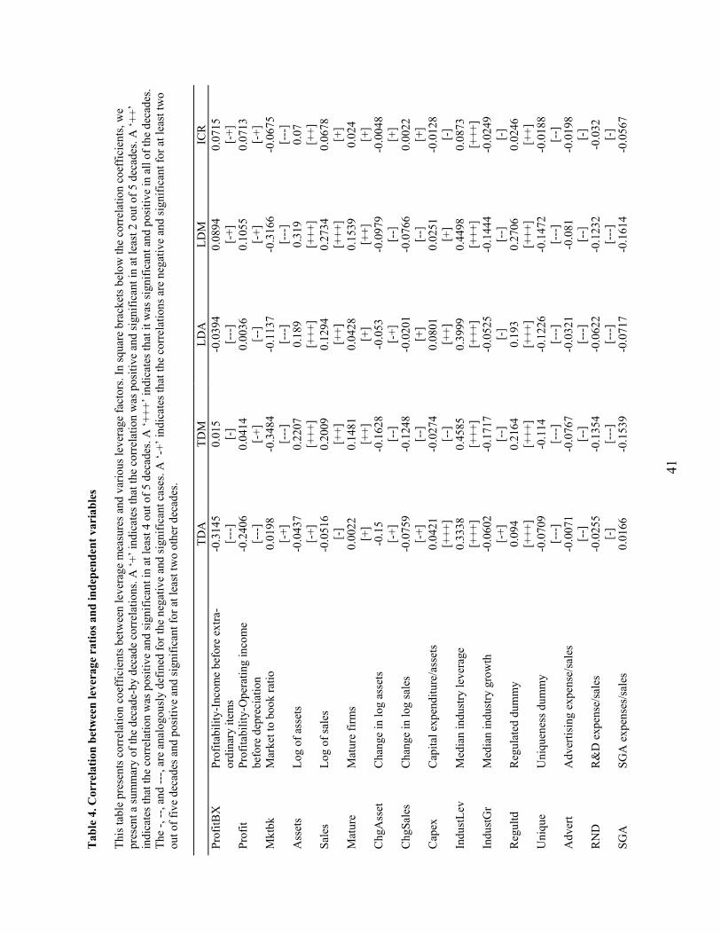
41

Tab

le 4

. Cor

rela

tion

betw

een

leve

rage

rat

ios a

nd in

depe

nden

t var

iabl

es

This

tabl

e pr

esen

ts c

orre

latio

n co

effic

ient

s bet

wee

n le

vera

ge m

easu

res a

nd v

ario

us le

vera

ge fa

ctor

s. In

squa

re b

rack

ets b

elow

the

corr

elat

ion

coef

ficie

nts,

we

pres

ent a

sum

mar

y of

the

deca

de-b

y de

cade

cor

rela

tions

. A �+

� ind

icat

es th

at th

e co

rrel

atio

n w

as p

ositi

ve a

nd si

gnifi

cant

in a

t lea

st 2

out

of 5

dec

ades

. A �+

+�

indi

cate

s tha

t the

cor

rela

tion

was

pos

itive

and

sign

ifica

nt in

at l

east

4 o

ut o

f 5 d

ecad

es. A

�+++

� ind

icat

es th

at it

was

sign

ifica

nt a

nd p

ositi

ve in

all

of th

e de

cade

s. Th

e -,

--, a

nd --

-, ar

e an

alog

ousl

y de

fined

for t

he n

egat

ive

and

sign

ifica

nt c

ases

. A �-

+� in

dica

tes t

hat t

he c

orre

latio

ns a

re n

egat

ive

and

sign

ifica

nt fo

r at l

east

two

out o

f fiv

e de

cade

s and

pos

itive

and

sign

ifica

nt fo

r at l

east

two

othe

r dec

ades

.

TD

A

TDM

LD

A

LDM

IC

R

Prof

itBX

Pr

ofita

bilit

y-In

com

e be

fore

ext

ra-

ordi

nary

item

s -0

.314

5

[---

] 0.

015

[-

] -0

.039

4

[---

] 0.

0894

[-

+]

0.07

15

[-+]

Pr

ofit

Prof

itabi

lity-

Ope

ratin

g in

com

e be

fore

dep

reci

atio

n -0

.240

6

[---

] 0.

0414

[-

+]

0.00

36

[--]

0.

1055

[-

+]

0.07

13

[-+]

M

ktbk

M

arke

t to

book

ratio

0.

0198

[-

+]

-0.3

484

[-

--]

-0.1

137

[-

--]

-0.3

166

[-

--]

-0.0

675

[-

--]

Ass

ets

Log

of a

sset

s -0

.043

7

[-+]

0.

2207

[+

++]

0.18

9

[+++

] 0.

319

[+

++]

0.07

[+

+]

Sale

s Lo

g of

sale

s -0

.051

6

[-]

0.20

09

[++]

0.

1294

[+

+]

0.27

34

[+++

] 0.

0678

[+

] M

atur

e M

atur

e fir

ms

0.00

22

[+]

0.14

81

[++]

0.

0428

[+

] 0.

1539

[+

+]

0.02

4

[+]

Chg

Ass

et

Cha

nge

in lo

g as

sets

-0

.15

[-

+]

-0.1

628

[-

-]

-0.0

53

[-+]

-0

.097

9

[--]

-0

.004

8

[+]

Chg

Sale

s C

hang

e in

log

sale

s -0

.075

9

[-+]

-0

.124

8

[--]

-0

.020

1

[+]

-0.0

766

[-

-]

0.00

22

[+]

Cap

ex

Cap

ital e

xpen

ditu

re/a

sset

s 0.

0421

[+

++]

-0.0

274

[-

-]

0.08

01

[++]

0.

0251

[+

] -0

.012

8

[-]

Indu

stLe

v M

edia

n in

dust

ry le

vera

ge

0.33

38

[+++

] 0.

4585

[+

++]

0.39

99

[+++

] 0.

4498

[+

++]

0.08

73

[+++

] In

dust

Gr

Med

ian

indu

stry

gro

wth

-0

.060

2

[-+]

-0

.171

7

[--]

-0

.052

5

[-]

-0.1

444

[-

-]

-0.0

249

[-

] R

egul

td

Reg

ulat

ed d

umm

y 0.

094

[+

++]

0.21

64

[+++

] 0.

193

[+

++]

0.27

06

[+++

] 0.

0246

[+

+]

Uni

que

Uni

quen

ess d

umm

y -0

.070

9

[---

] -0

.114

[-

--]

-0.1

226

[-

--]

-0.1

472

[-

--]

-0.0

188

[-

-]

Adv

ert

Adv

ertis

ing

expe

nse/

sale

s -0

.007

1

[--]

-0

.076

7

[--]

-0

.032

1

[---

] -0

.081

[-

-]

-0.0

198

[-

] R

ND

R

&D

exp

ense

/sal

es

-0.0

255

[-

] -0

.135

4

[---

] -0

.062

2

[---

] -0

.123

2

[---

] -0

.032

[-

] SG

A

SGA

exp

ense

s/sa

les

0.01

66

-0.1

539

-0

.071

7

-0.1

614

-0

.056

7

42

TDA

TD

M

LDA

LD

M

ICR

[+

] [-

--]

[---

] [-

--]

[--]

C

olltr

l C

olla

tera

l 0.

1552

[+

++]

0.33

02

[+++

] 0.

2278

[+

++]

0.34

12

[+++

] 0.

0516

[+

++]

Tang

Ta

ngib

ility

0.

1824

[+

++]

0.27

32

[+++

] 0.

3112

[+

++]

0.36

17

[+++

] 0.

0397

[+

+]

Inta

ng

Inta

ngib

le a

sset

s/as

sets

0.

1138

[+

++]

0.04

23

[++]

0.

1552

[+

++]

0.05

95

[++]

0.

0294

[+

+]

TaxR

ate

Top

tax

rate

-0

.031

3

[-]

0.10

8

[0]

0.00

21

[-]

0.11

6

[0]

0.00

62

[-]

NO

LCF

NO

L ca

rryf

orw

ards

/ass

ets

0.28

23

[+++

] -0

.057

1

[-+]

0.

0341

[+

+]

-0.1

049

[-

] -0

.059

1

[-]

Dep

r D

epre

ciat

ion/

asse

ts

0.20

49

[+]

0.04

07

[+]

0.09

61

[+]

0.00

99

[+]

-0.0

112

[-

] In

vTax

Cr

Inve

stm

ent t

ax c

redi

ts/a

sset

s 0.

0404

[+

+]

0.16

71

[++]

0.

1048

[+

+]

0.21

49

[++]

0.

0142

[0

] N

DTa

xSh

Non

debt

tax

shie

lds/

asse

ts

-0.3

009

[-

--]

0.02

62

[-]

-0.0

363

[-

-]

0.09

53

[-+]

0.

0694

[-

+]

Div

iden

d D

ivid

end

payi

ng d

umm

y -0

.132

4 [-

--]

0.01

65

[-+]

-0

.012

1

[-]

0.09

9

[-+]

0.

005

[-

+]

Loss

es

Loss

mak

ing

dum

my

0.07

99

[++]

-0

.117

5

[-+]

-0

.093

7

[-]

-0.1

995

[-

] -0

.372

3

[---

] R

atin

g In

vest

men

t gra

de d

ebt r

atin

g du

mm

y 0.

0074

[0

] 0.

0278

[-

] 0.

0512

[+

] 0.

0574

[+

] 0.

0097

[0

] ZS

core

Z-

Scor

e -0

.387

3

[--]

0.

0138

[-

-]

-0.0

776

[-

-]

0.07

41

[-+]

0.

0647

[-

+]

FCon

str

Kor

ajcz

yk/L

evy

dum

my

-0.0

12

[-+]

-0

.209

8

[--]

-0

.114

9

[-]

-0.2

041

[-

-]

-0.0

508

[-

+]

Stoc

kVar

V

aria

nce

of a

sset

retu

rns

-0.1

439

[-

] -0

.221

4

[--]

-0

.208

6

[--]

-0

.256

9

[--]

-0

.067

6

[-]

Stoc

kRet

C

umul

ativ

e an

nual

raw

retu

rns

-0.0

911

[-

-]

-0.1

957

[-

--]

-0.0

363

[-

--]

-0.1

304

[-

--]

-0.0

088

[-

] C

rspR

et

Cum

ulat

ive

annu

al m

arke

t ret

urns

-0

.008

8

[-]

-0.0

789

[-

--]

0.00

35

[+]

-0.0

568

[-

--]

-0.0

012

[0

] Te

rmSp

rd

Term

spre

ad

0.00

98

[-]

-0.0

725

[-

--]

-0.0

088

[-

] -0

.067

[-

--]

-0.0

022

[-

] Q

ualS

prd

Qua

lity

spre

ad

-0.0

415

[0

] 0.

0147

[+

] -0

.009

7

[0]

0.02

41

[+]

-0.0

163

[0

] TB

ill

Dis

coun

t rat

e 0.

0479

[+

+]

0.14

84

[+++

] 0.

0343

[+

+]

0.12

55

[+++

] 0.

041

[+

+]

43

TDA

TD

M

LDA

LD

M

ICR

M

grSe

nti

Log

purc

hasi

ng m

anag

ers i

ndex

-0

.027

6

[-]

-0.0

334

[-

-]

-0.0

148

[-

] -0

.019

5

[--]

-0

.018

3

[-]

Mac

roPr

of

Gro

wth

in p

rofit

afte

r tax

-Mac

ro

-0.0

114

[-

-]

-0.0

177

[-

-]

-0.0

096

[-

] -0

.012

2

[-]

-0.0

052

[0

] M

acro

Gr

Gro

wth

in G

DP

-0.0

303

[-

] -0

.075

7

[--]

-0

.020

3

[-]

-0.0

584

[-

-]

-0.0

21

[-]

NB

ER

NB

ER re

cess

ions

0.

0123

[-

] 0.

1205

[+

] 0.

0114

[0

] 0.

0959

[+

] 0.

0179

[+

]

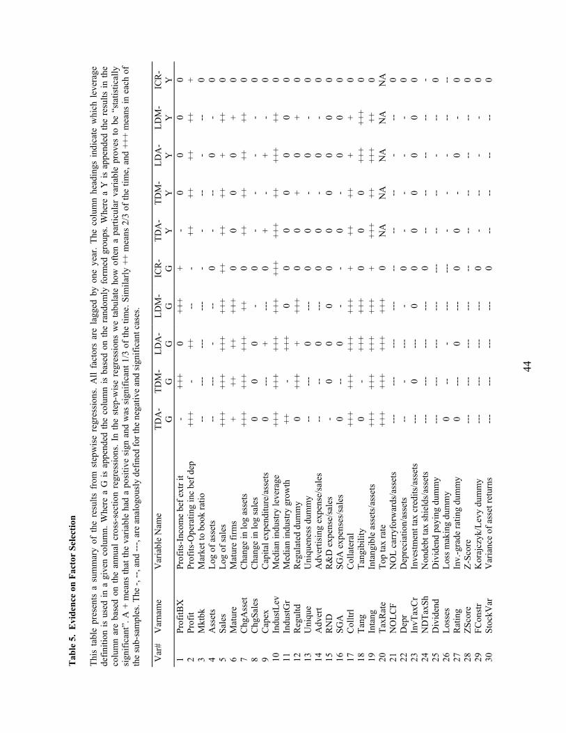
44

Tab

le 5

. E

vide

nce

on F

acto

r Se

lect

ion

Th

is t

able

pre

sent

s a

sum

mar

y of

the

res

ults

fro

m s

tepw

ise

regr

essi

ons.

All

fact

ors

are

lagg

ed b

y on

e ye

ar.

The

colu

mn

head

ings

ind

icat

e w

hich

lev

erag

e de

finiti

on is

use

d in

a g

iven

col

umn.

Whe

re a

G is

app

ende

d th

e co

lum

n is

bas

ed o

n th

e ra

ndom

ly f

orm

ed g

roup

s. W

here

a Y

is a

ppen

ded

the

resu

lts in

the

colu

mn

are

base

d on

the

annu

al c

ross

-sec

tion

regr

essi

ons.

In th

e st

ep-w

ise

regr

essi

ons

we

tabu

late

how

ofte

n a

parti

cula

r va

riabl

e pr

oves

to b

e �s

tatis

tical

ly

sign

ifica

nt�.

A +

mea

ns th

at th

e va

riabl

e ha

d a

posi

tive

sign

and

was

sig

nific

ant 1

/3 o

f the

tim

e. S

imila

rly +

+ m

eans

2/3

of t

he ti

me,

and

+++

mea

ns in

eac

h of

th

e su

b-sa

mpl

es. T

he -,

--, a

nd --

-, ar

e an

alog

ousl

y de

fined

for t

he n

egat

ive

and

sign

ifica

nt c

ases

. V

ar#

Var

nam

e V

aria

ble

Nam

e TD

A-

G

TDM

-G

LD

A-

G

LDM

-G

IC

R-

G

TDA

-Y

TD

M-

Y

LDA

-Y

LD

M-

Y

ICR

- Y

1

Prof

itBX

Pr

ofits

-Inc

ome

bef e

xtr i

t -

+++

0 ++

+ +

- 0

0 0

0 2

Prof

it Pr

ofits

-Ope

ratin

g in

c be

f dep

++

+ -

++

--

- ++

++

++

++

+

3 M

ktbk

M

arke

t to

book

ratio

--

--

- --

- --

- -

- --

-

--

0 4

Ass

ets

Log

of a

sset

s --

--

- -

--

0 -

--

0 -

0 5

Sale

s Lo

g of

sale

s ++

+ ++

+ ++

+ ++

+ ++

++

++

+

++

0 6

Mat

ure

Mat

ure

firm

s +

++

++

+++

0 0

0 0

+ 0

7 C

hgA

sset

C

hang

e in

log

asse

ts

+++

+++

+++

++

0 ++

++

++

++

0

8 C

hgSa

les

Cha

nge

in lo

g sa

les

0 0

0 -

0 -

- -

- 0

9 C

apex

C

apita

l exp

endi

ture

/ass

ets

0 --

- +

---

0 +

- +

- 0

10

Indu

stLe

v M

edia

n in

dust

ry le

vera

ge

+++

+++

+++

+++

+++

+++

++

+++

++

0 11

In

dust

Gr

Med

ian

indu

stry

gro

wth

++

-

+++

0 0

0 0

0 0

0 12

R

egul

td

Reg

ulat

ed d

umm

y 0

+++

+ ++

+ 0

0 +

0 +

0 13

U

niqu

e U

niqu

enes

s dum

my

--

---

0 --

- 0

0 -

0 -

0 14

A

dver

t A

dver

tisin

g ex

pens

e/sa

les

--

--

0 --

- 0

0 -

0 -

0 15

R

ND

R

&D

exp

ense

/sal

es

- 0

0 0

0 0

0 0

0 0

16

SGA

SG

A e

xpen

ses/

sale

s 0

--

0 -

- 0

- 0

0 0

17

Col

ltrl

Col

late

ral

+++

+++

+++

+++

+ ++

++

+

+ 0

18

Tang

Ta

ngib

ility

0

- ++

+ ++

+ 0

0 0

+++

+++

0 19

In

tang

In

tang

ible

ass

ets/

asse

ts

+++

+++

+++

+++

+ ++

+ ++

++

+ ++

0

20

TaxR

ate

Top

tax

rate

++

+ ++

+ ++

+ ++

+ 0

NA

N

A

NA

N

A

NA

21

N

OLC

F N

OL

carr

yfor

war

ds/a

sset

s --

- --

- --

- --

- --

--

--

-

--

0 22

D

epr

Dep

reci

atio

n/as

sets

--

-

---

- 0

- -

- -

0 23

In

vTax

Cr

Inve

stm

ent t

ax c

redi

ts/a

sset

s --

- 0

---

0 0

0 0

0 0

0 24

N

DTa

xSh

Non

debt

tax

shie

lds/

asse

ts

---

---

---

---

0 --

--

--

--

-

25

Div

iden

d D

ivid

end

payi

ng d

umm

y --

- --

- --

- --

- --

- --

--

-

--

0 26

Lo

sses

Lo

ss m

akin

g du

mm

y 0

--

- --

- --

- -

- -

--

--

27

Rat

ing

Inv.

-gra

de ra

ting

dum

my

0 --

- 0

---

0 0

- 0

- 0

28

ZSco

re

Z-Sc

ore

---

---

---

---

--

--

--

--

--

0 29

FC

onst

r K

oraj

czyk

/Lev

y du

mm

y --

- --

- --

- --

- 0

- --

-

- 0

30

Stoc

kVar

V

aria

nce

of a

sset

retu

rns

---

---

---

---

0 --

--

--

--

0

45

Var

# V

arna

me

Var

iabl

e N

ame

TDA

-G

TD

M-

G

LDA

-G

LD

M-

G

ICR

- G

TD

A-

Y

TDM

-Y

LD

A-

Y

LDM

-Y

IC

R-

Y

31

Stoc

kRet

C

umul

ativ

e an

nual

raw

retu

rns

0 --

- +

- 0

0 -

0 -

0 32

C

rspR

et

Cum

ulat

ive

annu

al m

arke

t ret

urns

0

++

0 ++

+

0 +

0 +

0 33

Te

rmSp

rd

Term

spre

ad

0 --

0

0 0

NA

N

A

NA

N

A

NA

34

Q

ualS

prd

Qua

lity

spre

ad

0 0

0 +

0 N

A

NA

N

A

NA

N

A

35

TBill

D

isco

unt r

ate

++

++

+ ++

+ ++

+ N

A

NA

N

A

NA

N

A

36

Mgr

Sent

i Lo

g pu

rcha

sing

man

ager

s ind

ex

0 ++

+ 0

+++

+ N

A

NA

N

A

NA

N

A

37

Mac

roPr

of

Gro

wth

in p

rofit

afte

r tax

-Mac

ro

0 -

0 0

0 N

A

NA

N

A

NA

N

A

38

Mac

roG

r G

row

th in

GD

P +

---

+ --

- 0

NA

N

A

NA

N

A

NA

39

N

BER

N

BER

rece

ssio

ns

0 +

0 ++

0

NA

N

A

NA

N

A

NA

46

Tab

le 6

. Evi

denc

e on

Fac

tor

Sele

ctio

n by

firm

cir

cum

stan

ces

This

tabl

e re

ports

a s

umm

ary

of th

e ex

plan

ator

y po

wer

of l

ever

age

fact

ors f

or v

ario

us c

lass

es o

f firm

s. Th

is ta

ble

is c

onst

ruct

ed in

two

step

s. In

the

first

ste

p, w

e ta

bula

te f

or t

he f

ive

leve

rage

mea

sure

s ho

w o

ften

a pa

rticu

lar

fact

or a

ppea

rs s

tatis

tical

ly s

igni

fican

t in

ten

sub

sam

ple

grou

ps a

nd i

n an

nual

cro

ss-s

ectio

n re

gres

sion

s. Fo

r ex

ampl

e, f

or e

ach

leve

rage

mea

sure

, we

assi

gn a

�+

(-)�

to a

fac

tor

if it

is p

ositi

ve (

nega

tive)

and

sta

tistic

ally

sig

nific

ant i

n at

leas

t 1/3

of

the

grou

ps fo

r gro

up re

gres

sion

s. W

e as

sign

a �+

+ (-

-)� i

f the

fact

or is

pos

itive

(neg

ativ

e) a

nd s

igni

fican

t in

at le

ast t

wo-

third

s of

the

regr

essi

ons

and

we

assi

gn �+

++

(---

)� if

the

fact

or is

pos

itive

(ne

gativ

e) a

nd s

igni

fican

t in

all o

f th

e re

gres

sion

s. W

e fo

llow

a s

imila

r pr

oced

ure

to s

umm

ariz

e th

e re

gres

sion

res

ults

for

ann

ual

cros

s se

ctio

n re

gres

sion

s. In

the

seco

nd s

tep,

we

aggr

egat

e th

ese

code

s ac

ross

the

five

leve

rage

mea

sure

s fo

r bot

h gr

oups

and

yea

rs. T

he th

eore

tical

max

imum

va

lue

a fa

ctor

can

hav

e is

eith

er 3

0+ o

r 30-

if th

e fa

ctor

is s

tatis

tical

ly s

igni

fican

t and

of a

con

sist

ent s

ign

in e

ach

of th

e 10

sub

sam

ple

regr

essi

ons

and

in e

ach

of

the

37 a

nnua

l cro

ss-s

ectio

nal r

egre

ssio

ns f

or a

ll fiv

e of

the

leve

rage

mea

sure

s. Th

e ta

ble

pres

ents

thes

e su

mm

arie

s fo

r al

l firm

s in

the

third

col

umn

and

for

vario

us c

lass

es o

f fir

ms.

The

clas

ses

we

exam

ine

incl

ude

(1)

divi

dend

-pay

ing

firm

s (d

ivid

end

payi

ng d

umm

y=1)

; (2

) no

n-di

vide

nd-p

ayin

g fir

ms

(div

iden

d-pa

ying

dum

my=

0); (

3) m

atur

e fir

ms (

if fir

ms h

ave

been

list

ed o

n C

ompu

stat

for 1

0 ye

ars o

r mor

e); (

4) y

oung

firm

s (if

firm

s hav

e be

en li

sted

on

Com

pust

at fo

r 5

year

s or

less

); (5

) sm

all f

irms

(if a

sset

s ar

e sm

alle

r tha

n th

e 33

rd p

erce

ntile

of a

ll C

ompu

stat

firm

s); (

6) la

rge

firm

s (if

ass

ets

are

larg

er th

an th

e 67

th p

erce

ntile

of

all C

ompu

stat

firm

s); (

7) lo

w M

/B fi

rms

(if th

e m

arke

t-to-

book

ass

ets

ratio

is s

mal

ler t

han

the

33rd

per

cent

ile o

f all

firm

s on

Com

pust

at);

(8) h

igh

M/B

firm

s (if

th

e m

arke

t-to-

book

ass

ets

ratio

is la

rger

than

the

67th

per

cent

ile o

f al

l Com

pust

at f

irms)

; (9

) lo

w p

rofit

firm

s (if

Pro

fit is

less

than

the

33rd

per

cent

ile o

f al

l C

ompu

stat

firm

s); (

10) h

igh-

prof

it fir

ms (

if Pr

ofit

is g

reat

er th

an th

e 67

th p

erce

ntile

of a

ll C

ompu

stat

firm

s).

Var

nam

e V

aria

ble

Nam

e A

ll Fi

rms

Div

. Pa

ying

N

on

Div

. Pa

ying

Mat

ure

Firm

s Y

oung

Fi

rms

Smal

l Fi

rms

Larg

e Fi

rms

Low

M

/B

Hig

h M

/B

Low

Pr

ofits

H

igh

Prof

its

Prof

itBX

Pr

ofits

-Inc

ome

bef.

extr.

item

s 7+

,2-

0+,1

3-

0+,2

- 4+

,4-

7+,3

- 3+

,1-

0+,1

0-

4+,0

- 5+

,3-

0+,2

- 0+

,8-

Prof

it Pr

ofits

-Ope

ratin

g in

c be

f. de

pr

14+,

4-

15+,

0-

13+,

1-

12+,

2-

14+,

3-

10+,

2-

12+,

4-

15+,

0-

19+,

0-

19+,

0-

24+,

0-

Mkt

bk

Mar

ket t

o bo

ok ra

tio

0+,1

8-

0+,1

0-

0+,1

2-

0+,1

7-

0+,1

9-

0+,1

2-

0+,1

1-

6+,6

- 0+

,16-

0+

,10-

0+

,16-

A

sset

s Lo

g of

ass

ets

0+,1

3-

0+,1

9-

7+,2

- 0+

,19-

1+

,13-

5+

,3-

0+,2

0-

0+,1

7-

4+,1

- 5+

,0-

0+,2

3-

Sale

s Lo

g of

sale

s 21

+,0-

21

+,0-

16

+,0-

21

+,0-

20

+,0-

6+

,0-

19+,

0-

21+,

0-

9+,0

- 13

+,0-

24

+,0-

M

atur

e M

atur

e fir

ms

9+,0

- 0+

,2-

7+,0

- 0+

,0-

NA

N

A

2+,0

- 1+

,0-

2+,0

- 0+

,0-

0+,0

- C

hgA

sset

C

hang

e in

log

asse

ts

19+,

0-

20+,

0-

8+,0

- 18

+,0-

18

+,0-

9+

,0-

16+,

0-

19+,

0-

5+,0

- 6+

,0-

14+,

0-

Chg

Sale

s C

hang

e in

log

sale

s 0+

,5-

1+,2

- 0+

,1-

0+,6

- 0+

,3-

0+,0

- 0+

,4-

0+,1

- 0+

,0-

0+,3

- 0+

,1-

Cap

ex

Cap

ital e

xpen

ditu

re/a

sset

s 3+

,8-

8+,0

- 2+

,9-

5+,3

- 5+

,7-

0+,3

- 8+

,2-

1+,0

- 2+

,0-

5+,0

- 2+

,12-

In

dust

Lev

Med

ian

indu

stry

leve

rage

25

+,0-

24

+,0-

21

+,0-

24

+,0-

26

+,0-

20

+,0-

24

+,0-

22

+,0-

21

+,0-

20

+,0-

25

+,0-

In

dust

Gr

Med

ian

indu

stry

gro

wth

5+

,1-

3+,2

- 1+

,1-

4+,1

- 3+

,2-

1+,0

- 1+

,0-

0+,0

- 3+

,0-

1+,0

- 0+

,0-

Reg

ultd

R

egul

ated

dum

my

9+,0

- 11

+,0-

2+

,0-

8+,0

- 8+

,0-

3+,0

- 8+

,0-

7+,0

- 4+

,0-

1+,0

- 4+

,0-

Uni

que

Uni

quen

ess d

umm

y 0+

,10-

0+

,12-

0+

,6-

0+,1

2-

0+,1

0-

0+,3

- 0+

,10-

0+

,4-

0+,0

- 0+

,3-

0+,3

- A

dver

t A

dver

tisin

g ex

pens

e/sa

les

0+,9

- 0+

,3-

1+,1

- 0+

,5-

0+,7

- 0+

,0-

0+,4

- 0+

,3-

0+,0

- 0+

,0-

0+,0

- R

ND

R

&D

exp

ense

/sal

es

0+,1

- 0+

,12-

0+

,1-

0+,8

- 0+

,2-

0+,0

- 0+

,10-

0+

,2-

0+,3

- 2+

,0-

0+,1

2-

SGA

SG

A e

xpen

ses/

sale

s 0+

,5-

1+,6

- 0+

,1-

1+,7

- 0+

,5-

0+,0

- 2+

,5-

0+,0

- 0+

,2-

0+,0

- 0+

,10-

C

olltr

l C

olla

tera

l 19

+,0-

18

+,0-

18

+,0-

19

+,0-

19

+,0-

15

+,0-

15

+,0-

18

+,0-

10

+,0-

14

+,0-

18

+,0-

Ta

ng

Tang

ibili

ty

12+,

1-

10+,

6-

10+,

0-

10+,

2-

10+,

1-

10+,

0-

9+,4

- 10

+,2-

10

+,0-

10

+,2-

10

+,1-

In

tang

In

tang

ible

ass

ets/

asse

ts

23+,

0-

17+,

0-

20+,

0-

20+,

0-

20+,

0-

19+,

0-

17+,

0-

20+,

0-

19+,

0-

20+,

0-

23+,

0-

TaxR

ate

Top

tax

rate

12

+,0-

12

+,0-

8+

,0-

12+,

0-

12+,

0-

7+,0

- 12

+,0-

4+

,0-

12+,

0-

9+,0

- 10

+,1-

47

Var

nam

e V

aria

ble

Nam

e A

ll Fi

rms

Div

. Pa

ying

N

on

Div

. Pa

ying

Mat

ure

Firm

s Y

oung

Fi

rms

Smal

l Fi

rms

Larg

e Fi

rms

Low

M

/B

Hig

h M

/B

Low

Pr

ofits

H

igh

Prof

its

NO

LCF

NO

L ca

rryf

orw

ards

/ass

ets

0+,2

1-

0+,2

- 0+

,15-

0+

,20-

0+

,20-

0+

,11-

1+

,3-

0+,1

3-

0+,1

6-

0+,7

- 0+

,25-

D

epr

Dep

reci

atio

n/as

sets

0+

,11-

0+

,11-

0+

,12-

0+

,11-

0+

,11-

0+

,1-

0+,7

- 0+

,7-

0+,2

- 0+

,4-

4+,4

- In

vTax

Cr

Inve

stm

ent t

ax c

redi

ts/a

sset

s 0+

,6-

2+,4

- 0+

,0-

0+,4

- 0+

,6-

0+,0

- 0+

,6-

0+,0

- 0+

,4-

0+,0

- 0+

,6-

ND

TaxS

h N

onde

bt ta

x sh

ield

s/as

sets

0+

,21-

0+

,24-

0+

,17-

0+

,19-

0+

,24-

0+

,14-

0+

,21-

0+

,22-

0+

,21-

0+

,20-

0+

,25-

D

ivid

end

Div

iden

d pa

ying

dum

my

0+,2

2-

0+,0

- 0+

,0-

0+,2

1-

0+,2

1-

0+,1

2-

0+,2

0-

0+,1

8-

0+,1

7-

0+,1

7-

0+,2

0-

Loss

es

Loss

mak

ing

dum

my

0+,1

6-

0+,2

2-

2+,7

- 0+

,18-

1+

,16-

0+

,5-

0+,1

5-

0+,1

8-

3+,5

- 0+

,4-

0+,1

4-

Rat

ing

Inv.

-gra

de ra

ting

dum

my

0+,8

- 3+

,0-

0+,1

0-

0+,8

- 0+

,8-

0+,0

- 2+

,1-

0+,6

- 0+

,0-

0+,0

- 1+

,2-

ZSco

re

Z-Sc

ore

0+,2

2-

0+,2

3-

0+,2

0-

0+,2

2-

0+,2

2-

0+,1

0-

0+,2

3-

0+,2

1-

0+,2

0-

0+,1

5-

0+,2

5-

FCon

str

Kor

ajcz

yk/L

evy

dum

my

0+,1

7-

0+,0

- 0+

,15-

0+

,14-

0+

,14-

0+

,8-

0+,6

- 0+

,6-

0+,1

5-

0+,1

2-

0+,1

0-

Stoc

kVar

V

aria

nce

of a

sset

retu

rns

0+,2

0-

0+,1

4-

0+,1

9-

0+,2

0-

0+,2

0-

0+,1

2-

0+,1

5-

0+,1

9-

0+,1

2-

0+,1

5-

0+,2

0-

Stoc

kRet

C

um. a

nnua

l raw

retu

rns

1+,6

- 2+

,5-

0+,7

- 1+

,5-

2+,6

- 0+

,3-

2+,9

- 0+

,4-

2+,0

- 0+

,3-

1+,1

- C

rspR

et

Cum

. ann

ual m

arke

t ret

urns

7+

,0-

3+,0

- 3+

,0-

3+,0

- 6+

,0-

1+,0

- 5+

,0-

3+,0

- 0+

,0-

3+,0

- 1+

,0-

Term

Sprd

Te

rm sp

read

0+

,2-

0+,4

- 0+

,3-

0+,3

- 0+

,2-

0+,3

- 0+

,8-

2+,1

- 0+

,1-

0+,0

- 0+

,4-

Qua

lSpr

d Q

ualit

y sp

read

1+

,0-

1+,0

- 0+

,1-

1+,0

- 0+

,2-

0+,0

- 0+

,0-

2+,0

- 0+

,0-

0+,0

- 0+

,5-

TBill

D

isco

unt r

ate

11+,

0-

11+,

0-

5+,0

- 11

+,0-

11

+,0-

0+

,1-

6+,0

- 4+

,0-

2+,0

- 5+

,0-

5+,0

- M

grSe

nti

Log

purc

h. m

anag

ers i

ndex

7+

,0-

7+,0

- 8+

,0-

8+,0

- 9+

,0-

5+,0

- 7+

,0-

6+,1

- 9+

,0-

6+,0

- 8+

,0-

Mac

roPr

of

Gro

wth

- agg

r. pr

ofit

afte

r tax

0+

,1-

2+,0

- 0+

,1-

2+,0

- 0+

,0-

0+,0

- 1+

,0-

0+,0

- 0+

,0-

0+,0

- 0+

,2-

Mac

roG

r G

row

th in

GD

P 2+

,6-

4+,5

- 0+

,7-

2+,6

- 2+

,6-

0+,2

- 0+

,5-

1+,4

- 0+

,4-

1+,6

- 4+

,2-

NB

ER

NB

ER re

cess

ions

3+

,0-

2+,0

- 0+

,0-

3+,0

- 3+

,0-

0+,0

- 3+

,0-

2+,0

- 2+

,0-

3+,0

- 0+

,0-

48

Tab

le 7

. Exp

lain

ing

Var

iatio

n Th

is ta

ble

repo

rts h

ow m

uch

varia

tion

in le

vera

ge m

easu

res

is e

xpla

ined

by

each

of t

he fa

ctor

s. �O

wn�

repo

rts th

e R

2 from

sim

ple

univ

aria

te re

gres

sion

s. Th

e �C

umul

ativ

e� re

ports

R

2 from

a re

gres

sion

that

incl

udes

the

varia

ble

liste

d, a

long

with

all

varia

bles

list

ed a

bove

it in

the

Tabl

e. T

he v

aria

bles

are

list

ed in

the

orde

r of t

he a

mou

nt o

f add

ition

al v

aria

tion

expl

aine

d. W

e st

art

with

the

reg

ress

ion

that

inc

lude

s al

l va

riabl

es. T

hat

R2 g

oes

in t

he c

umul

ativ

e co

lum

n at

the

bot

tom

of

the

Tabl

e. T

hen,

we

dele

te t

he v

aria

ble

that

has

pe

rfor

med

wor

st a

nd ru

n th

e re

gres

sion

with

the

rem

aini

ng v

aria

bles

. We

repo

rt th

at R

2 in th

e se

cond

to th

e bo

ttom

cel

l in

the

tabl

e. W

e th

en c

ontin

ue in

this

man

ner a

ll th

e w

ay u

p th

e ta

ble.

TD

A

TDA

TD

A

TDM

TD

M

TDM

LD

A

LDA

LD

A

LDM

LD

M

LDM

IC

R

ICR

IC

R

Var

iabl

e O

wn

R2

Cum

ul.

R2

Var

iabl

e O

wn

R2

Cum

ul.

R2

Var

iabl

e O

wn

R2

Cum

ul.

R2

Var

iabl

e O

wn

R2

Cum

ulR

2 V

aria

ble

Ow

n R

2 C

umul

R

2 ZS

core

0.

0877

0.

0877

In

dust

Lev

0.10

74

0.10

74

Indu

stLe

v 0.

1556

0.

1556

In

dust

Lev

0.19

46

0.19

46

Loss

es

0.01

09

0.01

09

Indu

stLe

v 0.

1074

0.

1883

M

ktbk

0.

0002

0.

2562

Ta

ng

0.09

31

0.18

84

Mkt

bk

0.08

85

0.24

15

Indu

stLe

v 0.

0075

0.

0161

Pr

ofit

0.02

99

0.19

01

Col

ltrl

0.02

41

0.27

27

Inta

ng

0.02

22

0.20

74

Tang

0.

1259

0.

2780

N

DTa

xSh

0.00

23

0.01

67

ND

TaxS

h 0.

0474

0.

2098

ZS

core

0.

0877

0.

2848

ZS

core

0.

0043

0.

1994

Sa

les

0.07

59

0.29

09

Mkt

bk

0.00

39

0.01

69

Col

ltrl

0.02

41

0.22

14

Sale

s 0.

0011

0.

2950

Sa

les

0.01

83

0.21

82

ND

TaxS

h 0.

0081

0.

3061

D

ivid

end

0.00

01

0.01

79

Inta

ng

0.01

46

0.23

85

Div

iden

d 0.

0138

0.

3162

D

ivid

end

0.00

00

0.23

29

Div

iden

d 0.

0116

0.

3173

TB

ill

0.00

18

0.01

88

Div

iden

d 0.

0138

0.

2483

TB

ill

0.00

30

0.31

96

Stoc

kVar

0.

0307

0.

2761

In

tang

0.

0038

0.

3193

Sa

les

0.00

40

0.01

89

TaxR

ate

0.00

02

0.25

74

Mgr

Sent

i 0.

0000

0.

3271

N

OLC

F 0.

0002

0.

2596

TB

ill

0.01

14

0.32

55

Inta

ng

0.00

09

0.01

82

Sale

s 0.

0011

0.

2729

N

DC

AST

0.

0474

0.

3323

C

olltr

l 0.

0494

0.

2653

M

grSe

nti

0.00

13

0.33

20

Col

ltrl

0.00

27

0.01

83

Mkt

bk

0.00

02

0.28

02

NO

LCF

0.04

81

0.32

33

TaxR

ate

0.00

02

0.26

66

Col

ltrl

0.11

11

0.33

39

SGA

0.

0028

0.

0185

N

OLC

F 0.

0481

0.

2925

In

tang

0.

0146

0.

3301

N

DTa

xSh

0.00

04

0.26

74

ZSco

re

0.00

40

0.33

41

Dep

r 0.

0001

0.

0187

St

ockV

ar

0.00

81

0.28

87

FCon

str

0.00

04

0.33

46

Prof

it 0.

0002

0.

2703

N

OLC

F 0.

0106

0.

3071

N

OLC

F 0.

0024

0.

0176

A

sset

s 0.

0000

0.

2917

Ta

xRat

e 0.

0002

0.

3386

M

ktbk

0.

0129

0.

2725

R

atin

g 0.

0035

0.

3108

ZS

core

0.

0025

0.

0170

C

hgA

sset

0.

0107

0.

2950

C

apex

0.

0023

0.

3417

C

hgA

sset

0.

0011

0.

2756

St

ockV

ar

0.05

30

0.32

06

Cap

ex

0.00

01

0.01

71

FCon

str

0.00

04

0.29

69

Prof

itBX

0.

0500

0.

3442

FC

onst

r 0.

0106

0.

2772

R

egul

td

0.07

38

0.32

36

Mgr

Sent

i 0.

0001

0.

0172

D

epr

0.02

39

0.29

78

Ass

ets

0.00

00

0.34

46

Dep

r 0.

0055

0.

2784

Lo

sses

0.

0382

0.

3265

C

rspR

et

0.00

00

0.01

81

Mac

roG

r 0.

0000

0.

2986

St

ockV

ar

0.00

81

0.36

05

Indu

stG

r 0.

0016

0.

2793

M

acro

Gr

0.00

01

0.32

93

Prof

itBX

0.

0026

0.

0182

In

vTax

Cr

0.00

19

0.29

71

Mac

roG

r 0.

0000

0.

3632

In

vTax

Cr

0.01

16

0.27

72

FCon

str

0.03

46

0.33

12

Rat

ing

0.00

01

0.01

83

Indu

stG

r 0.

0024

0.

2976

R

atin

g 0.

0002

0.

3653

M

atur

e 0.

0030

0.

2777

Pr

ofitB

X

0.00

81

0.33

31

Mac

roG

r 0.

0002

0.

0184

TB

ill

0.00

30

0.29

81

Uni

que

0.00

59

0.36

73

Stoc

kRet

0.

0020

0.

2810

Ta

xRat

e 0.

0153

0.

3354

Te

rmSp

rd

0.00

01

0.01

85

RN

D

0.00

14

0.29

85

Reg

ultd

0.

0106

0.

3690

SG

A

0.00

52

0.28

13

Cap

ex

0.00

27

0.33

72

Uni

que

0.00

04

0.01

86

Uni

que

0.00

59

0.29

88

Adv

ert

0.00

00

0.37

03

Mac

roPr

of

0.00

00

0.28

14

Uni

que

0.02

22

0.33

83

InvT

axC

r 0.

0002

0.

0186

Lo

sses

0.

0053

0.

2991

C

hgA

sset

0.

0107

0.

3715

TB

ill

0.00

13

0.28

16

Prof

it 0.

0093

0.

3393

R

ND

0.

0003

0.

0187

A

dver

t 0.

0000

0.

2992

St

ockR

et

0.00

87

0.37

44

Loss

es

0.00

73

0.28

18

Adv

ert

0.00

57

0.34

02

Prof

it 0.

0026

0.

0187

M

atur

e 0.

0006

0.

2993

M

atur

e 0.

0006

0.

3752

R

egul

td

0.04

07

0.28

20

Chg

Ass

et

0.00

58

0.34

04

TaxR

ate

0.00

01

0.01

88

Prof

itBX

0.

0500

0.

2994

Te

rmSp

rd

0.00

00

0.37

59

Rat

ing

0.00

30

0.28

21

Mat

ure

0.02

59

0.34

11

Stoc

kVar

0.

0034

0.

0187

C

hgSa

les

0.00

23

0.30

18

Crs

pRet

0.

0001

0.

3765

C

apex

0.

0080

0.

2823

N

BER

0.

0054

0.

3413

N

BER

0.

0002

0.

0188

N

BER

0.

0002

0.

3019

Ta

ng

0.03

28

0.37

70

Prof

itBX

0.

0004

0.

2824

C

rspR

et

0.00

23

0.34

19

Qua

lSpr

d 0.

0000

0.

0188

R

egul

td

0.01

06

0.30

19

SGA

0.

0001

0.

3775

U

niqu

e 0.

0165

0.

2825

A

sset

s 0.

1080

0.

3423

FC

onst

r 0.

0021

0.

0188

M

grSe

nti

0.00

00

0.30

20

NB

ER

0.00

02

0.37

79

Mac

roG

r 0.

0000

0.

2828

St

ockR

et

0.01

26

0.34

39

RN

D

0.00

10

0.01

88

Cap

ex

0.00

23

0.30

21

Loss

es

0.00

53

0.37

82

Crs

pRet

0.

0000

0.

2829

R

ND

0.

0148

0.

3441

A

sset

s 0.

0047

0.

0188

Ta

ng

0.03

28

0.30

21

Indu

stG

r 0.

0024

0.

3785

A

sset

s 0.

0416

0.

2830

Te

rmSp

rd

0.00

70

0.34

44

Mat

ure

0.00

08

0.01

89

SGA

0.

0001

0.

3022

D

epr

0.02

39

0.37

88

Adv

ert

0.00

08

0.28

30

SGA

0.

0236

0.

3446

C

hgSa

les

0.00

00

0.01

89

49

TDA

TD

A

TDA

TD

M

TDM

TD

M

LDA

LD

A

LDA

LD

M

LDM

LD

M

ICR

IC

R

ICR

V

aria

ble

Ow

n R

2 C

umul

. R

2 V

aria

ble

Ow

n R

2 C

umul

. R

2 V

aria

ble

Ow

n R

2 C

umul

. R

2 V

aria

ble

Ow

n R

2 C

umul

R2

Var

iabl

e O

wn

R2

Cum

ul

R2

Qua

lSpr

d 0.

0009

0.

3022

C

hgSa

les

0.00

23

0.38

02

Chg

Sale

s 0.

0001

0.

2838

C

hgSa

les

0.00

35

0.34

53

Indu

stG

r 0.

0004

0.

0189

Te

rmSp

rd

0.00

00

0.30

22

Mac

roPr

of

0.00

00

0.38

04

RN

D

0.00

43

0.28

38

Dep

r 0.

0000

0.

3455

C

hgA

sset

0.

0001

0.

0189

C

rspR

et

0.00

01

0.30

22

Prof

it 0.

0299

0.

3805

Q

ualS

prd

0.00

00

0.28

38

Indu

stG

r 0.

0116

0.

3456

M

acro

Prof

0.

0000

0.

0189

St

ockR

et

0.00

87

0.30

31

Qua

lSpr

d 0.

0009

0.

3806

Te

rmSp

rd

0.00

04

0.28

38

InvT

axC

r 0.

0446

0.

3452

R

egul

td

0.00

06

0.01

89

Rat

ing

0.00

02

0.30

31

InvT

axC

r 0.

0019

0.

3805

N

BER

0.

0002

0.

2838

M

acro

Prof

0.

0000

0.

3452

Ta

ng

0.00

17

0.01

89

Mac

roPr

of

0.00

00

0.30

31

RN

D

0.00

14

0.38

05

Mgr

Sent

i 0.

0000

0.

2838

Q

ualS

prd

0.00

20

0.34

52

Stoc

kRet

0.

0001

0.

0190

50

Tab

le 8

. A

Cor

e M

odel

of L

ever

age

This

tabl

e re

ports

the

estim

ated

coe

ffic

ient

s fro

m re

gres

sion

s of l

ever

age

mea

sure

s on

Tier

1 a

nd T

ier 2

fact

ors.

The

t-sta

tistic

s are

repo

rted

belo

w th

e co

effic

ient

s in

pare

nthe

ses.

The

elas

ticiti

es a

re re

porte

d in

squa

re b

rack

ets.

TD

A

TDA

TD

A

TDM

TD

M

TDM

LD

A

LDA

LD

A

LDM

LD

M

LDM

In

terc

ept

0.03

7 (1

5.3)

0.

039

(14.

1)

0.02

8

(5.0

) 0.

027

(11.

6)

0.06

0 (1

9.3)

-0

.042

(6

.7)

-0.0

50

(27.

4)

-0.0

41

(18.

5)

-0.0

08

(1.7

) -0

.060

(2

9.8)

-0

.031

(1

1.9)

-0

.080

(1

5.0)

In

dust

Lev

0.49

8 (8

7.6)

[0

.44]

0.47

8 (7

7.1)

[0

.45]

0.44

8 (7

2.6)

[0

.42]

0.59

6 (1

07.8

) [0

.48]

0.54

4 (7

8.5)

[0

.45]

0.51

2 (7

5.2)

[0

.42]

0.41

5 (9

7.9)

[0

.53]

0.38

1 (7

5.6)

[0

.50]

0.35

0 (7

0.2)

[0

.46]

0.49

3 (1

05.1

) [0

.55]

0.43

7 (7

4.0)

[0

.49]

0.40

7 (6

9.5)

[0

.46]

ZS

core

-0

.025

(1

30.6

) [-

0.13

]

-0.0

27

(89.

3)

[-0.

21]

-0.0

35

(67.

2)

[-0.

28]

-0.0

13

(66.

9)

[-0.

06]

-0.0

18

(53.

3)

[-0.

13]

-0.0

22

(37.

7)

[-0.

15]

-0.0

09

(64.

5)

[-0.

07]

-0.0

15

(60.

2)

[-0.

16]

-0.0

27

(65.

2)

[-0.

30]

-0.0

09

(54.

1)

[-0.

06]

-0.0

14

(47.

1)

[-0.

13]

-0.0

21

(42.

1)

[-0.

20]

Sale

s 0.

014

(39.

0)

[0.0

5]

0.01

3 (3

5.2)

[0

.05]

0.01

1 (2

8.6)

[0

.04]

0.02

0 (6

0.0)

[0

.07]

0.02

0 (4

6.6)

[0

.07]

0.01

8 (4

1.9)

[0

.06]

0.01

5 (5

5.8)

[0

.08]

0.01

5 (4

9.0)

[0

.08]

0.01

3 (4

0.0)

[0

.07]

0.02

1 (7

2.1)

[0

.10]

0.02

0 (5

6.8)

[0

.10]

0.01

9 (5

0.4)

[0

.09]

D

ivid

end

-0.0

81

(52.

8)

[-0.

14]

-0.0

71

(45.

1)

[-0.

14]

-0.0

80

(50.

2)

[-0.

16]

-0.0

88

(59.

6)

[-0.

14]

-0.0

88

(50.

2)

[-0.

16]

-0.1

04

(58.

9)

[-0.

18]

-0.0

49

(42.

8)

[-0.

12]

-0.0

43

(33.

5)

[-0.

12]

-0.0

48

(37.

4)

[-0.

14]

-0.0

46

(36.

7)

[-0.

10]

-0.0

48

(32.

4)

[-0.

12]

-0.0

59

(39.

1)

[-0.

14]

Inta

ng

0.32

8 (4

8.7)

[0

.06]

0.34

5 (4

6.7)

[0

.06]

0.33

9 (4

5.2)

[0

.06

0.21

8 (3

3.4)

[0

.04]

0.23

1 (2

7.9)

[0

.04]

0.26

4 (3

1.8)

[0

.04]

0.31

3 (6

2.1)

[0

.08]

0.32

7 (5

4.4)

[0

.09]

0.29

5 (4

8.6)

[0

.08]

0.22

5 (4

0.6)

[0

.05]

0.24

6 (3

4.9)

[0

.06]

0.25

5 (3

5.8)

[0

.06]

M

ktbk

-0

.007

(1

9.9)

[-

0.04

]

-0.0

09

(21.

0)

[-0.

05]

-0.0

07

(15.

6)

[-0.

04]

-0.0

34

(97.

6)

[-0.

18]

-0.0

43

(89.

4)

[-0.

21]

-0.0

38

(77.

0)

[-0.

19]

-0.0

04

(15.

2)

[-0.

03]

-0.0

05

(15.

6)

[-0.

04]

-0.0

05

(12.

8)

[-0.

04]

-0.0

21

(71.

4)

[-0.

15]

-0.0

28

(68.

4)

[-0.

19]

-0.0

25

(59.

5)

[-0.

17]

Col

ltrl

0.22

0 (6

5.9)

[0

.43]

0.21

7 (5

9.2)

[0

.46]

0.20

1 (5

4.6)

[0

.43]

0.24

4 (7

5.5)

[0

.44]

0.24

1 (5

9.0)

[0

.45]

0.22

1 (5

4.3)

[0

.41]

0.18

1 (7

2.4)

[0

.51]

0.18

2 (6

1.2)

[0

.54]

0.16

7 (5

6.1)

[0

.49]

0.21

1 (7

6.7)

[0

.52]

0.21

0 (6

0.2)

[0

.53]

0.19

3 (5

5.2)

[0

.49]

St

ockV

ar

-9.8

89

(22.

6)

[-0.

04]

-9.7

53

(20.

1)

[-0.

04]

-8.8

98

(25.

1)

[-0.

06]

-9.0

43

(21.

7)

[-0.

05]

NO

LCF

-0.0

33

(25.

0)

[-0.

02]

-0.0

46

(30.

7)

[-0.

03]

-0.0

34

(32.

0)

[-0.

03]

-0.0

39

(30.

3)

[-0.

03]

FCon

str

-0.0

48

(16.

8)

[-0.

01]

-0.0

83

(26.

0)

[-0.

02]

-0.0

32

(13.

8)

[-0.

01]

-0.0

50

(18.

2)

[-0.

01]

51

TD

A

TDA

TD

A

TDM

TD

M

TDM

LD

A

LDA

LD

A

LDM

LD

M

LDM

Pr

ofit

-0.0

47

(9.2

) [-

0.02

]

-0.1

74

(30.

9)

[-0.

07]

0.02

8

(6.9

) [0

.02]

-0.0

82

(16.

9)

[-0.

04]

Chg

Ass

et

0.02

4 (1

1.2)

[0

.01]

0.01

1 (4

.8)

[<0.

01]

0.03

2 (1

8.4)

[0

.01]

0.02

0

(9.8

) [0

.01]

Ta

xRat

e

0.

171

(13.

8)

[0.2

9]

0.39

5 (2

9.0)

[0

.57]

0.07

5

(7.5

) [0

.17]

0.25

2 (2

1.5)

[0

.50]

TB

ill

0.00

1

(3.9

) [0

.03]

0.00

2 (5

.0)

[0.0

4]

0.00

1

(2.7

) [0

.02]

0.00

2

(6.1

) [0

.05]

N

umbe

r of o

bs.

124,

051

81,8

49

81,8

49

122,

255

81,3

93

81,3

93

124,

090

81,8

70

81,8

70

122,

255

81,3

93

81,3

93

AIC

-2

5,14

7.2

-45,

190.

0 -4

7,35

6.4

-35,

684.

1 -2

7,31

0.2

-31,

517.

4 -9

7,57

8.2

-79,

238.

1 -8

2,12

8.8

-75,

587.

4 -5

3,38

4.7

-56,

429.

3 B

IC

-25,

069.

4 -4

5,11

5.4

-47,

216.

7 -3

5,60

6.4

-27,

235.

7 -3

1,37

7.8

-97,

500.

3 -7

9,16

3.6

-81,

989.

1 -7

5,50

9.7

-53,

310.

2 -5

6,28

9.7

Adj

R-s

quar

ed

0.26

0.

26

0.28

0.

32

0.31

0.

34

0.23

0.

24

0.26

0.

31

0.28

0.

31

52

Tab

le 9

. Con

trol

ling

For

Mis

sing

Obs

erva

tions

. Th

is ta

ble

repo

rts e

stim

ates

bas

ed o

n th

e us

e of

Mul

tiple

Impu

tatio

n fo

r the

mis

sing

dat

a. T

he im

puta

tion

is d

one

usin

g th

e M

etho

d of

Mar

kov

Cha

in M

onte

C

arlo

, as i

mpl

emen

ted

in S

AS

8.2

PRO

C M

I. W

e im

pute

10

times

and

dis

card

the

initi

al 1

000

obse

rvat

ions

for t

he �

burn

in�

perio

d. T

he t-

stat

istic

s are

repo

rted

in p

aren

thes

es. T

he �

betw

een�

impu

tatio

n va

rianc

es a

re re

porte

d in

cur

ly b

rack

ets a

nd th

e �w

ithin

� im

puta

tion

varia

nces

are

repo

rted

in sq

uare

bra

cket

s. * A

ll va

rianc

es e

xcep

t tho

se fo

r Sto

ckVa

r are

mul

tiplie

d by

106 .

TD

A

TDA

TD

M

TDM

LD

A

LDA

LD

M

LDM

In

terc

ept

0.03

9 (1

6.49

) {1

.308

}

[4.2

89]

0.03

5

(6.6

1)

{6.9

08}

[21.

212]

0.03

4

(16.

35)

{0.9

71}

[3

.310

]

-0.2

1 (-

4.30

) {7

.631

} [1

6.05

2]

-0.0

53

(-30

.88)

{0

.611

}

[2.2

23]

0.00

9

(2.5

3)

{2.0

47}

[10.

927]

-0.0

55

(-29

.05)

{1

.052

}

[2.3

63]

-0.0

54

(-13

.48)

{4

.188

} [1

1.54

7]

Indu

stLe

v 0.

614

(1

18.3

3)

{4.5

89}

[21.

899]

0.57

9

(105

.18)

{7

.429

} [2

2.13

7]

0.64

6

(136

.20)

{5

.107

} [1

6.90

3]

0.61

1

(122

.23)

{7

.472

} [1

6.75

2]

0.49

7

(141

.25)

{0

.921

} [1

1.35

2]

0.46

9

(126

.20)

{2

.167

} [1

1.40

4]

0.52

6

(133

.35)

{3

.170

} [1

2.06

8]

0.49

6

(121

.12)

{4

.305

} [1

2.05

1]

ZSco

re

-0.0

23

(-15

4.56

) {0

.003

}

[0.0

19]

-0.0

25

(-69

.17)

{0

.062

}

[0.0

61]

-0.0

12

(-89

.56)

{0

.003

}

[0.0

15]

-0.0

12

(-46

.44)

{0

.026

}

[0.0

46]

-0.0

08

(-71

.95)

{0

.002

} [0

.010

]

-0.0

12

(-48

.44)

{0

.028

}

[0.0

32]

-0.0

07

(-64

.94)

{0

.002

}

[0.0

11]

-0.0

10

(-38

.51)

{0

.025

}

[0.0

33]

Sale

s 0.

012

(3

5.37

) {0

.033

}

[0.0

89]

0.00

8

(20.

25)

{0.0

51}

[0

.100

]

0.02

0

(59.

21)

{0.0

44}

[0

.069

]

0.01

8

(49.

87)

{0.0

52}

[0

.075

]

0.01

4

(61.

26)

{0.0

85}

[0

.046

]

0.01

1

(42.

65)

{0.0

12}

[0

.051

]

0.02

1

(85.

42)

{0.0

09}

[0.0

49]

0.01

9

(71.

66)

{0.0

14}

[0

.054

] D

ivid

end

-0.0

90

(-59

.86)

{0

.366

}

[1.8

90]

-0.1

07

(-69

.95)

{0

.350

}

[1.9

94]

-0.0

91

(-57

.66)

{0

.952

}

[1.4

59]

-0.1

11

(-69

.48)

{0

.959

}

[1.5

09]

-0.0

54

(-51

.89)

{0

.088

}

[0.9

80]

-0.0

64

(-60

.58)

{0

.081

} [1

.027

]

-0.0

49

(-41

.50)

{0

.329

}

[1.0

42]

-0.0

62

(-51

.05)

{0

.358

}

[1.0

86]

Inta

ng

0.35

1 (5

4.50

) {7

.100

} [3

3.67

2]

0.36

0

(53.

25)

{10.

151}

[3

4.48

9]

0.21

3 (3

5.47

) {9

.113

} [2

5.98

9]

0.23

1 (3

7.28

) {1

1.05

8}

[26.

098]

0.34

4

(72.

06)

{4.8

29}

[17.

454]

0.32

4

(67.

00)

{5.1

29}

[17.

766]

0.23

5

(46.

39)

{6.3

77}

[18.

555]

0.23

3

(45.

69)

{6.5

91}

[18.

774]

M

ktbk

-0

.009

(-

23.9

9)

{0.0

55}

[0

.094

]

-0.0

09

(-19

.17)

{0

.087

}

[0.1

03]

-0.0

33

(-10

8.96

) {0

.018

}

[0.0

72]

-0.0

32

(-95

.11)

{0

.030

}

[0.0

78]

-0.0

05

(-20

.07)

{0

.019

} [0

.049

]

-0.0

05

(-18

.59)

{0

.023

}

[0.0

53]

-0.0

21

(-78

.41)

{0

.015

}

[0.0

52]

-0.0

20

(-70

.70)

{0

.023

}

[0.0

56]

Col

ltrl

0.20

2

(69.

04)

{0.8

39}

[7

.718

]

0.18

7

(62.

51)

{0.9

94}

[7.8

81]

0.21

3 (7

6.58

) {1

.596

}

[5.9

57]

0.19

7

(71.

49)

{1.5

00}

[5.9

64]

0.16

5

(76.

25)

{0.6

22}

[4

.001

]

0.15

7 (7

2.99

) {0

.535

} [4

.060

]

0.18

4

(73.

55)

{1.7

97}

[4

.253

]

0.17

5

(70.

62)

{1.6

83}

[4

.290

]

53

TD

A

TDA

TD

M

TDM

LD

A

LDA

LD

M

LDM

St

ockV

ar

-1

5.18

4 (-

22.7

0)

{0.2

96}*

[0.1

22]*

-1

2.39

7

(-23

.71)

{0

.165

}* [0

.092

]*

-1

2.56

4

(-30

.12)

{0

.101

}* [0

.063

]*

-1

1.10

7

(-25

.25)

{0

.116

}* [0

.066

]* N

OLC

F

0.00

5

(4.1

5)

{0.7

73}

[0

.489

]

-0

.009

(-

10.4

4)

{0.3

68}

[0

.370

]

-0

.006

(-

8.38

) {0

.311

}

[0.2

52]

-0

.010

(-

13.3

7)

{0.2

85}

[0

.266

] FC

onst

r

-0.4

6

(-19

.72)

{1

.436

}

[3.8

03]

-0

.71

(-

36.6

9)

{0.7

95}

[2

.878

]

-0

.037

(-

23.2

7)

{0.4

58}

[1

.959

]

-0

.047

(-

29.0

0)

{0.5

04}

[2

.070

] Pr

ofit

0.

017

(5.1

0)

{2.7

71}

[8

.141

]

-0

.094

(-

27.7

9)

{4.7

39}

[6

.161

]

0.

012

(5

.10)

{1

.078

}

[4.1

94]

-0

.058

(-

21.0

5)

{2.9

36}

[4

.432

] C

hgA

sset

0.00

2

(0.9

6)

{0.8

15}

[2

.229

]

0.

004

(2

.59)

{0

.646

}

[1.6

87]

0.

019

(1

5.18

) {0

.429

} [1

.148

]

0.

017

(12.

81)

{0.5

97}

[1

.213

] Ta

xRat

e

0.16

2

(14.

41)

{14.

556}

[1

11.0

00]

0.

235

(2

2.64

) {2

1.91

3}

[84.

038]

0.

001

(0

.17)

{9

.019

} [5

7.20

8]

0.

091

(10.

65)

{11.

003}

[6

0.45

3]

TBill

0.00

1

(3.1

8)

{0.0

21}

[0

.068

]

0.

004

(1

6.09

) {0

.018

}

[0.0

52]

-0

.000

4

(-1.

65)

{0.0

13}

[0

.035

]

0.

003

(1

3.94

) {0

.007

}

[0.0

37]

54

Tab

le 1

0.

Cor

e L

ever

age

regr

essi

ons b

y de

cade

s Th

is ta

ble

repo

rts th

e es

timat

ed c

oeff

icie

nts f

rom

regr

essi

ons o

f TD

A o

n Ti

er 1

and

Tie

r 2 fa

ctor

s. Th

e t-s

tatis

tics a

re re

porte

d be

low

the

coef

ficie

nts i

n pa

rent

hese

s. Th

e el

astic

ities

are

repo

rted

in sq

uare

bra

cket

s.

Onl

y Ti

er 1

fact

ors

Bot

h Ti

er 1

and

Tie

r 2 fa

ctor

s

1960

-196

9 19

70-1

979

1980

-198

9 19

90-2

000

1960

-196

9 19

70-1

979

1980

-198

9 19

90-2

000

Inte

rcep

t 0.

184

(1

5.0)

0.

151

(2

6.1)

0.

065

(1

2.2)

0.

009

(2

.0)

0.16

5

(8.9

) 0.

217

(2

5.8)

0.

109

(6

.9)

-0.1

56

(1.5

) In

dust

Lev

0.54

5

(31.

9)

[0.4

9]

0.40

9

(41.

8)

[0.4

1]

0.48

6

(38.

1)

[0.4

5]

0.42

1

(38.

9)

[0.3

9]

0.51

9

(30.

7)

[0.4

7]

0.40

2

(41.

9)

[0.4

0]

0.47

0

(37.

0)

[0.4

3]

0.40

0

(36.

7)

[0.3

7]

ZSco

re

-0.0

45

(26.

4)

[-0.

49]

-0.0

48

(66.

0)

[-0.

50]

-0.0

32

(54.

1)

[-0.

24]

-0.0

21

(47.

1)

[-0.

12]

-0.0

35

(18.

9)

[-0.

39]

-0.0

39

(45.

8)

[-0.

40]

-0.0

36

(36.

5)

[-0.

27]

-0.0

31

(35.

0)

[-0.

18]

Sale

s 0.

005

(4

.4)

[0.0

2]

0.01

2

(20.

7)

[0.0

5]

0.01

3

(17.

8)

[0.0

5]

0.01

5

(21.

5)

[0.0

6]

0.00

5

(3.9

) [0

.02]

0.00

9

(14.

0)

[0.0

3]

0.01

1

(14.

8)

[0.0

4]

0.01

2

(16.

2)

[0.0

5]

Div

iden

d -0

.047

(9

.2)

[-0.

15]

-0.0

64

(29.

5)

[-0.

17]

-0.0

76

(25.

0)

[-0.

15]

-0.0

69

(22.

7)

[-0.

10]

-0.0

46

(5.8

) [-

0.15

]

-0.0

71

(30.

9)

[-0.

18]

-0.0

82

(26.

4)

[-0.

16]

-0.0

75

(24.

5)

[-0.

11]

Inta

ng

0.50

0

(13.

9)

[0.0

4]

0.33

9

(21.

7)

[0.0

4]

0.40

1

(22.

3)

[0.0

5]

0.36

6

(34.

2)

[0.1

2]

0.44

6

(12.

6)

[0.0

4]

0.36

6

(24.

0)

[0.0

4]

0.38

6

(21.

4)

[0.0

5]

0.33

2

(30.

5)

[0.1

1]

Mkt

bk

-0.0

12

(8.7

) [-

0.08

]

-0.0

14

(14.

3)

[-0.

05]

-0.0

07

(8.8

) [-

0.04

]

-0.0

08

(11.

2)

[-0.

06]

-0.0

07

(4.4

) [-

0.05

]

-0.0

10

(9.5

) [-

0.04

]

-0.0

05

(6.2

) [-

0.03

]

-0.0

06

(9.0

) [-

0.05

] C

olltr

l 0.

113

(8

.6)

[0.2

9]

0.17

4

(28.

5)

[0.4

0]

0.21

1

(30.

7)

[0.4

4]

0.22

6

(35.

7)

[0.4

4]

0.13

9

(10.

8)

[0.3

5]

0.17

1

(28.

5)

[0.3

9]

0.20

4

(29.

3)

[0.4

3]

0.21

2

(33.

1)

[0.4

1]

Stoc

kVar

1.

338

(0

.3)

[<0.

01]

-29.

067

(2

0.0)

[-

0.08

]

-12.

333

(1

1.2)

[-

0.05

]

-6.3

57

(10.

9)

[-0.

05]

NO

LCF

0.06

3

(3.2

) [<

0.01

]

0.02

6

(4.1

) [<

0.01

]

-0.0

26

(9.3

) [-

0.02

]

-0.0

25

(12.

6)

[-0.

03]

FCon

str

-0.0

26

(2.8

) [-

0.01

]

-0.0

28

(5.5

) [<

0.00

]

-0.0

74

(12.

5)

[-0.

01]

-0.0

54

(10.

8)

[-0.

02]

55

O

nly

Tier

1 fa

ctor

s B

oth

Tier

1 a

nd T

ier 2

fact

ors

19

60-1

969

1970

-197

9 19

80-1

989

1990

-200

0 19

60-1

969

1970

-197

9 19

80-1

989

1990

-200

0 Pr

ofit

-0.2

64

(9.5

) [-

0.18

]

-0.2

73

(24.

2)

[-0.

16]

-0.0

64

(7.2

) [-

0.02

]

0.01

6

(1.9

) [<

0.01

] C

hgA

sset

0.

147

(1

6.5)

[0

.04]

0.10

0

(19.

1)

[0.0

1]

0.02

9

(7.3

) [0

.01]

0.01

0

(3.1

) [<

0.01

] Ta

xRat

e

N

A

NA

-0

.004

(0

.1)

[-0.

01]

0.57

8

(2.0

) [0

.84]

TB

ill

0.00

3

(0.9

) [0

.05]

-0.0

01

(0.6

) [-

0.01

]

0.00

1

(1.7

) [0

.03]

0.00

6

(5.0

) [0

.11]

N

umbe

r of o

bs.

4,70

7 22

,895

26

,318

27

,929

4,

707

22,8

95

26,3

18

27,9

29

AIC

-6

,536

.3

-26,

349.

5 -1

0,42

4.2

-9,2

60.2

-6

,887

.8

-27,

512.

8 -1

0,90

2.7

-9,7

36.5

B

IC

-6,4

84.6

-2

6,28

5.2

-10,

358.

8 -9

,194

.2

-6,7

97.4

-2

7,40

0.3

-10,

780.

0 -9

,613

.0

Adj

R-s

quar

ed

0.44

0.

37

0.25

0.

25

0.49

0.

40

0.26

0.

26