Capital Structure, Investment, and Fire Sales

Douglas Gale Piero Gottardi SRC Discussion Paper No 23

November 2014

ISSN 2054-538X

Abstract We study a dynamic general equilibrium model in which firms choose their investment level and their capital structure, trading off the tax advantages of debt against the risk of costly default. The costs of bankruptcy are endogenously determined, as bankrupt firms are forced to liquidate their assets, resulting in a fire sale if the market is illiquid. When the corporate income tax rate is positive, firms have a unique optimal capital structure. In equilibrium firms default with positive probability and their assets are liquidated at fire-sale prices. The equilibrium not only features underinvestment but is also constrained inefficient. In particular there is too little debt and too little default. Keywords: Debt, equity, capital structure, default, market liquidity, constrained inefficiency, incomplete markets JEL classification: D5, D6, G32, G33 This paper is published as part of the Systemic Risk Centre’s Discussion Paper Series. The support of the Economic and Social Research Council (ESRC) in funding the SRC is gratefully acknowledged [grant number ES/K002309/1]. Douglas Gale is Professor of Economics and Director of Research in the Brevan Howard Centre for Financial Research, Imperial College London, and a Research Associate at the Systemic Risk Centre, London School of Economics Piero Gottardi is Professor of Economics at the Department of Economics, European University Institute (since September 2008, on leave from Universita’ di Venezia) Published by Systemic Risk Centre The London School of Economics and Political Science Houghton Street London WC2A 2AE All rights reserved. No part of this publication may be reproduced, stored in a retrieval system or transmitted in any form or by any means without the prior permission in writing of the publisher nor be issued to the public or circulated in any form other than that in which it is published. Requests for permission to reproduce any article or part of the Working Paper should be sent to the editor at the above address. © Douglas Gale, Piero Gottardi submitted 2014

Capital Structure, Investment, and Fire Sales

Douglas Gale Piero Gottardi

August 30, 2014

Abstract

We study a dynamic general equilibrium model in which firms choose their investment level

and their capital structure, trading off the tax advantages of debt against the risk of costly

default. The costs of bankruptcy are endogenously determined, as bankrupt firms are forced

to liquidate their assets, resulting in a fire sale if the market is illiquid. When the corporate

income tax rate is positive, firms have a unique optimal capital structure. In equilibrium

firms default with positive probability and their assets are liquidated at fire-sale prices.

The equilibrium not only features underinvestment but is also constrained inefficient. In

particular there is too little debt and too little default.

JEL Nos: D5, D6, G32, G33

Keywords: Debt, equity, capital structure, default, market liquidity, constrained ineffi-

ciency, incomplete markets

1 Introduction

The financial crisis of 2007-2008 and the recent sovereign debt crisis in Europe have focused

attention on the macroeconomic consequences of debt financing. In this paper, we turn our

attention to the use of debt finance in the corporate sector and study the general equilibrium

effects of debt finance on investment and growth. We show that, when markets are incomplete

and firms use debt and equity to finance investment, there is underinvestment and debt

finance is too low in equilibrium.

At the heart of our analysis is the determination of the firm’s capital structure. In

the classical model of Modigliani and Miller (1958), capital structure is indeterminate. To

obtain a determinate capital structure, subsequent authors appealed to market frictions, such

as distortionary taxes, bankruptcy costs, and agency costs.1 We follow this tradition and

examine an environment where the optimal capital structure balances the tax advantages

of debt against the risk of costly bankruptcy. More precisely, debt has an advantage over

equity because interest payments are deductible from corporate income, while dividends and

retained earnings are not. At the same time, the use of debt generates the risk of bankruptcy

which is costly for the firm because it forces the firm to sell its assets at fire-sale prices. The

firm balances the perceived costs and benefits of debt and equity in choosing its capital

structure. We show that these costs and benefits support an interior optimum of the firm’s

capital structure decision.

We consider an infinite-horizon economy, where firms choose their production and invest-

ment in long lived capital goods and are subject to productivity shocks. We focus primarily

on firms’ decisions and abstract from distributional issues by assuming there is a representa-

tive consumer. Firms finance the purchase of capital by issuing debt and equity. We assume

that markets are incomplete in two respects. First, there are no markets for contingent claims

allowing firms to insure against the risk of bankruptcy. Second, when a firm is bankrupt

1See, for example, Barnea, Haugen and Senbet (1981), Bradley, Jarrell and Kim (1984), Brennan and

Schwartz (1978), Dammon and Green (1987), Fischer, Heinkel and Zechner (1989), Kim (1982), Leland and

Toft (1996), Miller (1977), and Titman (1984) and Titman and Wessels (1988).

1

- that is, fails to pay its debtors or to renegotiate its debt - the liquidation of its assets is

subject to a finance constraint that causes assets to be sold at fire-sale prices, i.e., at less

than their fundamental value.

In our model, both the corporate income tax and the cost of bankruptcy represent a pure

redistribution of resources rather than a real resource cost for the economy. The corporate

income tax revenue is returned to consumers in the form of lump sum transfers. Similarly,

the fire sale of assets constitutes a transfer of value to the shareholders of the firms that buy

the assets of bankrupt firms, rather than a deadweight cost. Since there is a representative

consumer, this “redistribution” has no effect on welfare. Nonetheless, a rational, value-

maximizing manager of a competitive firm will perceive the tax as a cost of using equity

finance and the risk of a fire sale in bankruptcy as a cost of using debt. These perceived

costs determine the firm’s financing decisions, act like a tax on capital, and distort the firm’s

investment decision.

As a baseline, consider the case where the corporate income tax rate is zero. In that case,

the competitive equilibrium allocation is Pareto efficient and the firms’ capital structure is

indeterminate.2 In other words, with a zero corporate income tax rate, the finance constraint

never binds and bankruptcy does not result in fire sales. By contrast, when the corporate

income tax rate is positive, competitive equilibria have quite different properties. They are

not just Pareto inefficient, exhibiting underinvestment; they are also constrained inefficient.

Also, the optimal capital structure of firms is uniquely determined in equilibrium, each firm

uses positive amounts of risky debt and equity as sources of finance and faces a positive

probability of costly bankruptcy. So many features of the equilibrium change when the

corporate tax rate becomes positive because the tax interacts with the incompleteness of

markets and the finance constraint to generate endogenous costs of bankruptcy.

The intuition for the second property is simple. If the probability of bankruptcy were

2To be precise, for each individual firm any combination of debt and equity is optimal. There is however

a constraint on the aggregate amount of debt in the economy, which has to be small enough that fire sales

do not occur.

2

zero or if bankrupt firms could be liquidated with no loss of value, then firms would use 100%

debt finance to avoid the corporate income tax. But, in equilibrium, we will show that 100%

debt finance is inconsistent with both a zero probability of bankruptcy and the absence of

fire sales, together with the optimality of firms’ decisions.

A similar argument shows that some debt has to be used in equilibrium. If firms used

100% equity finance, there would be no bankruptcy. Then a single firm could issue a small

amount of debt and benefit from the tax hedge, without causing a fire sale and hence without

the risk of costly bankruptcy. Uniqueness of the optimal capital structure follows from the

fact that a rational manager equates the marginal costs of debt and equity financing in equi-

librium and we show that, under reasonable conditions, the marginal costs are increasing.3

The constrained inefficiency of the equilibrium is the result of a pecuniary externality.

The tax on equity reduces the return on capital and causes underinvestment in equilibrium.

In equilibrium each firm sets its capital structure so that the benefit of a marginal increase

in its debt level, in terms of lower tax paid by the firm, just offsets the increase in expected

bankruptcy costs.4 However, if all firms were to increase their use of debt, the liquidation

price of defaulting firms would drop, and hence the profits of any firm buying these assets

when solvent increase. This effect offsets the increase in expected costs when the firm is

bankrupt. As a result, an increase in the debt level of all firms would lower the tax paid and

increase the return on capital and hence also investment and welfare. The fact that each

firm is a price taker leads it to overestimate the costs of debt financing, whereas the planner

takes into account the change in prices when all firms increase the use of debt. This is the

source of the pecuniary externality. Note that this externality arises even in the presence of a

3We don’t wish to claim too much for this result, of course. The optimal capital structure is unique only

within a given (symmetric) equilibrium. In general, the capital structure depends on the equilibrium, which

in turn depends on the model parameters, including policy parameters such as the tax rate. But note that

the Modigliani-Miller theorem also holds for a given equilibrium of a given model.4The cost of increasing the firm’s debt level has two components. First, the probability of going bankrupt

and having to liquidate assets in a fire sale increases. Second, the probability of making capital gains by

buying assets of other firms in a fire sale is reduced.

3

representative consumer. Consumers collectively own all the assets, tax revenues are returned

to consumers, and firms end up holding the same assets after liquidation. Nonetheless, we

find that individual firms’ decisions are distorted and this imposes a welfare cost on the

economy.

We should point out that, as a result of this externality, in the environment considered

there is too little bankruptcy risk and too little debt financing in equilibrium. This appears

to contradict the common intuition that firms have an incentive to use too much debt. Our

analysis shows the importance of a careful evaluation of the costs of firms’ default and of the

reallocation of assets among them which takes place in this event, illustrating a novel effect

of fire sales. The actual costs of default — and hence of debt relative to equity financing

— may prove to be lower than the costs privately perceived by firms, as firms also benefit

from this reallocation and the opportunity to acquire assets at low prices and these prices

are lower when the probability of default is higher. This misperception induces firms to rely

too little on debt compared to other sources of funding for which the risk of default is lower.

We believe this effect is particularly relevant in markets where the firms purchasing assets

at fire-sale prices are the same firms running the risk of default.

1.1 Related literature

The classical literature on the firm’s investment decision excludes external finance constraints

and bankruptcy costs and uses adjustment costs to explain the reliance of investment on To-

bin’s (see Eberly, Rebelo and Vincent, 2008, for a contemporary example). The new wave

literature on investment, exemplified by Sundaresan, Wang and Yang (2014) and Bolton,

Chen and Wang (2011), incorporates financing frictions of various types, such as a cost of

external funds, liquidity constraints and costs of liquidating the firm’s assets. Hackbarth

and Mauer (2012) then also allow for multiple debt issues with possibly different seniority.

These papers study the investment and financing decisions of an individual firm in partial

equilibrium.

A few papers consider instead, like our work, dynamic general equilibrium models with

4

several heterogeneous firms making optimal investment and financing decisions. Gomes and

Schmid (2010) and Miao and Wang (2010) study an environment fairly close to ours: they

also examine a representative agent economy where firms’ investment can be financed with

debt or equity, subject to a similar structure of costs. The liquidation cost, in the event

of default is exogenous in their set-up, whereas it is endogenously determined in ours by

the equilibrium price of liquidated assets. Also, they focus on the numerical analysis of an

equilibrium for a specification of the model aimed to match the persistence and volatility

of output growth, as well as credit spreads, while we provide a qualitative characterization

of equilibria and their welfare properties. The links between firms’ credit risk and their

leverage and investment decisions across the business cycle are examined by Kuehn and

Schmid (2011) in a partial equilibrium model with similar costs of financing.

The macroeconomic literature has emphasized the role of external finance constraints in

the business cycle. The financial accelerator model (Bernanke and Gertler, 1989; Bernanke,

Gilchrist and Gertler, 1999; Kiyotaki and Moore, 1997) shows that shocks to firm equity or

the value of collateral can restrict borrowing and amplify business cycle fluctuations. Our

focus is rather different: we consider an environment where financial frictions take the form

of costs of debt or equity financing rather than borrowing constraints. We also emphasize the

factors that determine the firm’s choice of capital structure and the implications for welfare

and regulatory interventions.

Pecuniary externalities play a key role in our welfare analysis. It has been well known

since the mid-eighties that pecuniary externalities have an impact on welfare in the presence

of market incompleteness, information asymmetries, or other frictions (Arnott and Stiglitz,

1986; Greenwald and Stiglitz, 1986; Geanakoplos and Polemarchakis, 1986). It is interesting

to contrast our constrained inefficiency result to the ones obtained by Lorenzoni (2008) (see

also Bianchi, 2011, Korinek, 2012, Gersbach and Rochet, 2012) in a financial accelerator

model of the kind discussed in the previous paragraph, where firms’ borrowing is constrained

by the future value of their assets. These authors show that equilibria may display excessive

borrowing, since a reduction in borrowing and investment allows to reduce the misallocation

5

costs of selling some of the firms’ assets in order to absorb negative shocks. In contrast we

show the inefficiency of the firms’ capital structure decisions in equilibrium in an environment

where firms are not constrained by the level of their collateral, but face some (endogenous)

costs of using alternative sources of funding. We find that an increase in the use of debt

relative to equity allows firms to lower their cost of funds, since the liquidation of the assets

of bankrupt firms at fire-sale prices constitutes not only a cost for a firm when bankrupt but

also a benefit for the same firm when solvent which firms fail to properly internalize.

The interaction between illiquidity and incompleteness of asset markets is also studied

in the literature on banking and financial crises. For models of fire sales and their impact

on bank portfolios, see Allen and Gale (2004a, 2004b). A similar process of renegotiation of

the debt of firms was considered by Gale and Gottardi (2011) in a static model in which, by

assumption, all investment was 100% debt financed.

The rest of the paper is organized as follows. In Section 2 we describe the primitives of

the model and characterize the first-best allocation. In Section 3 we describe the structure

of markets available specifying financial frictions and examine the decision problems of firms

and consumers. Section 4 defines competitive equilibria and establishes various fundamen-

tal properties. Section 5 shows that equilibria are inefficient and exhibit underinvestment.

Moreover, it shows that they are also constrained inefficient and the capital structure cho-

sen by firms exhibit too little debt. The concluding section discusses the robustness of the

results and extensions of the model. All proofs are collected in the appendix to this paper.

Extensions and additional results are contained in Appendix B, available online.

2 The Economy

We consider an infinite-horizon production economy. Time is described by a countable

sequence of dates, = 0 1 . At each date there are two goods, a perishable consumption

good and a durable capital good.

6

2.1 Consumers

There is a unit mass of identical, infinitely-lived consumers. The consumption stream of the

representative consumer is denoted by c = (0 1 ) ≥ 0, where is the amount of theconsumption good consumed at date . For any c ≥ 0, the representative consumer’s utilityis denoted by (c) and given by

(c) =

∞X=0

() (1)

where 0 1 and : R+ → R has the usual properties: it is 2 and such that 0 () 0

and 00 () 0 for any ≥ 0.

2.2 Production

There are two production sectors in the economy. In one, capital is produced using the

consumption good as an input. In the other, the consumption good is produced using the

capital good as an input.

Capital goods sector There is a unit mass of firms operating the technology for producing

capital. If ≥ 0 is the amount of the consumption good used as an input at date , theoutput is () ≥ 0 units of capital at the end of the period, where (·) is a 2 function

satisfying 0 () 0 and 00 () 0, for any ≥ 0, as well as the Inada conditions,

lim→0 0 () =∞ and lim→∞ 0 () = 0.

Consumption goods sector The technology for producing the consumption good uses

capital as an input and exhibits constant returns to scale. Production in this sector is

undertaken by a continuum of firms subject to independent stochastic depreciation rates.

Each unit of capital good used as an input by firm at an arbitrary date produces

(instantaneously) 0 units of output and becomes units after production takes place.

The random variables are assumed to be i.i.d. across firms as well as over time with

mean , support ∈ [0 1] and a continuous p.d.f. () We denote the c.d.f. by () and

7

the only other condition we impose on the distribution of is that the hazard rate()

1− () is

increasing.

2.3 Feasible allocations

At date 0, there is an initial stock of capital goods 0 0. To characterize the allocations

attainable in this economy the heterogeneity among firms and the idiosyncratic depreciation

shocks can be ignored since production can be diversified across the large number of firms.

By the law of large numbers convention, there is no aggregate uncertainty and the aggregate

depreciation rate is constant, with a fraction of the capital stock remaining each period

after depreciation. Thus a total amount of ≥ 0 units of capital goods at date produces units of consumption and leaves, after depreciation, units of capital goods to be used

next period.

A (symmetric) allocation is thus given by a sequence { }∞=0 that specifies theconsumption , capital , and investment at each date . The allocation { }∞=0 isfeasible if, for every date = 0 1 , it satisfies non-negativity,

( ) ≥ 0 (2)

attainability for the consumption good,

+ ≤ (3)

and the law of motion for capital,

+1 = + () (4)

together with the initial condition 0 = 0.

It follows from the assumptions regarding the technology for producing the capital good

that there exists a unique level of the capital stock, 0 ∞, satisfying the condition

³´=¡1−

¢.

8

When the capital stock at the beginning of a period is equal to , if all the current output

of the consumption good is used for investment the amount of capital available at the end of

the period remains constant, equal to . It is then straightforward to show that constitutes

an upper bound on the permanently feasible levels of the stock of capital.

Proposition 1 At any feasible allocation { }∞=0, we have lim sup→∞ ≤ .

As a corollary, is an upper bound on the levels of consumption and investment that can

be maintained indefinitely:

lim sup→∞

≤ lim sup→∞

≤

2.4 Efficient allocations

A first-best, socially optimal allocation maximizes the utility of the representative consumer

within the set of feasible allocations. More precisely, it is a sequence { }∞=0 that solvesthe problem of maximizing the representative consumer’s utility (1) subject to the feasibility

constraints (2), (3), and (4).

To characterize the properties of the first best, consider the necessary and sufficient

conditions for an interior solution¡

¢ À 0 = 0 1 of this problem. For

some non-negative multipliers {( )}∞=0, the allocation©¡

¢ª∞=0must satisfy

the conditions

0¡

¢=

+1+ +1 =

and

0 ¡

¢=

for every , together with the feasibility conditions (2-4) and the initial condition 0 = 0.

The boundedness property established above implies that the transversality condition

lim→∞

∞X=

() = 0

9

is automatically satisfied.

Much of our analysis focuses on steady states, that is on allocations such that

( ) = ( )

for all . It is interesting to see what the above first-order conditions imply for an optimal

steady state:

Proposition 2 At an optimal steady state, the capital stock is given by

=¡

¢1−

(5)

where ∗ is determined by

1− =

1

0 () (6)

Condition (6) has a natural interpretation in terms of marginal costs and benefits. The

marginal revenue of a unit of capital at the end of period 0 is

1− = + 2+ +

−1+

because it produces −1

units of the consumption good at each date 0 and the present

value of that consumption is −1

. The marginal cost of a unit of capital is 10() units

of consumption at date 0. So the optimality condition (6) requires the equality of marginal

cost and marginal revenue.

3 An incomplete markets economy

In this section we specify the structure of markets available in this economy and study the

decision problems of individual firms and consumers.

3.1 Firms and Markets

In the capital goods sector, since production is instantaneous and no capital is used, firms

simply maximize current profits in each period.

10

In the consumption sector, firms use capital, are infinitely lived and choose their in-

vestment level and financing strategy each period in the available markets. Firms are ex

ante identical, but subject to idiosyncratic depreciation shocks each period. Their ex post

heterogeneity cannot be ignored when we study their investment and financing decisions.

In a frictionless environment, where firms have access to a complete set of contingent

markets to borrow against their future income stream and hedge the idiosyncratic depreci-

ation shocks, the first-best allocation can be decentralized, in the usual way, as a perfectly

competitive equilibrium. In what follows, we consider instead an environment with financial

frictions, where there are no markets for contingent claims, firms are financed exclusively

with debt and equity and their output is sold in spot markets. In this environment as we

will see the first best is typically not attainable.

In the presence of uncertainty regarding the amount and value of a firm’s capital in the

subsequent period, debt financing gives rise to the risk of bankruptcy. This may be costly

because, in the event of default, a firm is required to liquidate its assets by selling them to

firms that remain solvent. These firms, though solvent, may be finance-constrained. When

this happens, there will be a fire sale, in which assets are sold for less than their full economic

value.

Equity financing, by contrast, entails no bankruptcy risk. The disadvantage of equity

is that firms must pay a (distortionary) tax on equity’s returns. We assume for simplicity

that the revenue of the tax on equity is used to make an equal lump sum transfer to all

consumers.

Both sources of funding, debt and equity, entail some costs for firms in the consump-

tion good sector. Firms choose their optimal capital structure in each period, that is, the

composition of outstanding debt and equity, by trading off the relative costs and benefits.

Given the CRTS property of the technology, the size of individual firms and the mass of

firms active in the consumption good sector are indeterminate. Moreover, since there will

be bankruptcy of existing firms and we allow for entry of new firms, the mass of active firms

may change over time. To simplify the description of equilibrium, we will focus our attention

11

on the case where a combination of entry and exit maintains the mass of firms equal to unity

and firms adjust their size so that each has the same amount of capital. Given the inherent

indeterminacy of equilibrium in the consumption goods sector, this assumption entails no

essential loss of generality and allows us to describe the evolution of the economy in terms

of a representative firm with capital stock .

At the initial date = 0, we assume that all capital is owned by firms in the consumption

good sector and that each of these firms has been previously financed entirely by equity.

Each consumer has an equal shareholding in each firm in the two sectors.

In what follows we shall focus our attention on the case where all firms’ debt has a

maturity of one period, so that the entire debt is due for repayment one period after it is

issued. Alternatively, we could have assumed that debt has a maturity of periods. In that

case the repayment due each period would be smaller. However, debt with longer maturity

also creates a moral hazard problem for creditors, because creditors have little power over

a firm as long as it pays in any period the required interest and principal. Hence equity

holders could enrich themselves at the expense of bond holders, paying themselves large

dividends by selling off capital until the firm is worthless. To address this problem long-term

bond contracts typically contain multiple covenants controlling the behavior of the firm. For

instance, covenants might restrict the firm’s ability to issue new debt, require the firm to

maintain an adequate ratio of earnings to interest payments, the so-called interest coverage

ratio, or to maintain the value of its assets in relation to the value of debt. If any of those

covenants is violated, the firm is technically in default and the repayment of the entire debt

is due immediately, which forces a renegotiation of the debt, similarly to the case of one

period bonds. In Appendix B, we show how the model can be extended to the special case of

perpetual bonds, where covenants give rise to default precisely as it occurs with one-period

bonds.

To analyze the firms’ decision formally we must first describe in more detail the structure

of markets and the timing of the debt renegotiation process leading possibly to default and

liquidation.

12

3.2 Renegotiation and default

Each date is divided into three sub-periods, labeled , , and .

A. In the first sub-period (), the production of the consumption good occurs and the

depreciation shock of each firm , , is realized. Also, the debt liabilities of each

firm are due. The firm has three options: it can repay the debt, renegotiate (“roll

over”) the debt, or default and declare bankruptcy. Renegotiation is modeled by a

game described in the next section. If renegotiation succeeds the firm remains solvent

and may then distribute its earnings to equity holders or retain them to finance new

purchases of capital.

B. In the intermediate sub-period (), the market opens where bankrupt firms can sell

their assets (their capital). A liquidity constraint applies, so that only agents with

ready cash, either solvent firms who retained earnings in sub-period or consumers

who received dividends in sub—period , can purchase the assets on sale. Let denote

the market price of the liquidated capital.

C. In the final sub-period (), the production of capital goods occurs. The profits of the

firms who operate in this sector are distributed to the consumers who own them. In

addition, debt holders of defaulting firms receive the proceeds of the liquidation sales in

sub-period B. The taxes on equity’s returns are due and the lump sum transfers to con-

sumers are also made in this sub-period. All other markets open, spot markets, where

the consumption and capital goods are traded, at the prices 1 and , respectively, as

well as asset markets, where debt and equity issued by firms (both surviving and newly

formed) to acquire capital are traded. The consumers buy and sell these securities in

order to fund future consumption and rebalance their portfolios. Equilibrium requires

that ≤ ; if no firm buys capital at the price and capital goods are in

excess supply in sub-period , contradicting the equilibrium conditions.

13

Note that agents face no liquidity constraint in the markets in sub-period . We can

interpret the fact that this constraint only applies to the markets for liquidated assets in

sub-period as portraying the haste with which the firms’ assets need to be sold after a

default. It can also be taken as an institutional feature of the bankruptcy process that does

not apply to other markets.

Bankruptcy procedures are source of numerous possible frictions (see Bebchuk, 1988;

Aghion, Hart and Moore, 1992; Shleifer and Vishny, 1992). In the present model, we focus

on one potential source of market failure, the so-called finance constraint, which requires

buyers to pay for their purchases of assets with the funds (cash) available to them, not with

the issue of IOUs. Hence the potential buyer who values the assets most highly may not

be able to raise enough finance to purchase the assets at their full economic value. This is

the cost of bankruptcy in the environment considered, which is endogenously determined in

equilibrium.5

We believe that our model of capital markets, with a clear distinction between liquidation

markets, represented by sub-period where only cash is accepted, and normal markets,

represented by sub-period where firms have complete access to external finance and there

is no liquidity constraint, is a reasonable approximation of reality. It is generally accepted

that capital markets are not perfect and it is costly, also in terms of time, for firms to obtain

external finance. A firm with sufficient time available may find it feasible to raise finance

for new capital goods by issuing debt and/or equity. In contrast, when a distressed firm

sells assets in a fire sale, firms in the same industry don’t have the time to obtain external

finance and have to rely on retained earnings to purchase these assets.6 The distinction

between markets for liquidated assets, where assets have to sold in a hurry, and normal

asset markets is obviously a matter of degree. Here, we have made the distinction sharper

than it is in reality by assuming the market for liquidated capital goods is “cash only,”

while firms in the other market have “free” access to external finance. This makes the model

5As further discussed in Section 5.2, we could allow for an additional, deadweight cost of bankruptcy,

with no substantial change in the results.6A model of this process is found in Shleifer and Vishny (1992).

14

tractable, without distorting reality too much, but the distinction could be weakened without

substantial qualitative change.

3.2.1 Sub-period A: The renegotiation game

Consider a firm with units of capital and an outstanding debt with face value 7 at

the beginning of period . The firm produces units of the consumption good, learns the

realization of its depreciation shock and must then choose whether to repay the debt or

try to renegotiate it. The renegotiation process that occurs in sub-period between the

firm and the creditors who purchased the firm’s bonds at − 1 is represented by a two-stagegame.

S1 The firm makes a “take it or leave it” offer to the bond holders to rollover the debt,

replacing each unit of the maturing debt with face value with a combination of

equity and debt maturing the following period. The new face value of the debt, +1,

determines the firm’s capital structure since equity is just a claim to the residual value.

S2 The creditors simultaneously accept or reject the firm’s offer.

Two conditions must be satisfied in order for renegotiation to succeed. First, a majority

of the creditors must accept the offer. Second, the rest of the creditors must be paid off

in full. If either condition is not satisfied, the renegotiation fails and the firm is declared

bankrupt. In that event, all the assets of the firm are frozen, nothing is distributed until

the capital stock has been liquidated (sold in the market). After liquidation, the sale price

of the liquidated assets is distributed to the bond holders in sub-period . Obviously, there

is nothing left for the shareholders in this case. Hence default is always involuntary: a firm

acting so as to maximize its market value will always repay or roll over the debt unless it is

unable to do so.

7Here and in what follows, it is convenient to denote by the face value of the debt issued per unit of

capital acquired.

15

We show next that there is an equilibrium of this renegotiation game where renegotiation

succeeds if and only if

≤ (+ ) (7)

that is, if the value of the firm’s equity is negative when its capital is evaluated at its

liquidation price . Note that the condition is independent of .

Consider, with no loss of generality, the case of a firm with one unit of capital, i.e., = 1,

and take an individual creditor holding debt with face value . If he rejects the offer and

demands to be repaid immediately, he receives in sub-period . With this payment, since

we said ≤ , we can assume without loss of generality that he purchasesunits of capital

in sub-period . Similarly, if the firm manages to roll over its debt, we can assume it retains

its cashflow and purchases units of capital in sub-period . Then it will have

+

units of capital at the start of sub-period . Therefore the most that the firm can offer the

creditor is a claim to an amount of capital + at the beginning of sub-period , with

market value

³+

´. The firm’s offer will be accepted only if the creditor rejecting the

offer ends up with no more capital than by accepting. Hence the firm is only able to make

an offer that is accepted if

≤

+

which is equivalent to (7).

If (7) is satisfied, there exists a sub-game perfect equilibrium of the renegotiation game

in which the firm makes an acceptable offer worth units of capital at the end of the

period to the creditors and all of them accept. To see this, note first that the shareholders

receive a non-negative payoff from rolling over the debt, whereas they get nothing in the

event of default. Second, the creditors will accept the offer of because they cannot get

a higher payoff by deviating and rejecting it, and they will not accept a lower offer. Thus,

we have the following simple result.

Proposition 3 There exists a sub-game perfect equilibrium of the renegotiation game in

which the debt is renegotiated if and only if (7) is satisfied.

16

Proposition 3 leaves open the possibility that renegotiation may fail even if (7) is satisfied.

Indeed it is the case that if every other creditor rejects the offer, it is optimal for a creditor

to reject the offer because a single vote has no effect. In the sequel, we ignore this trivial

coordination failure among lenders and assume that renegotiation succeeds whenever (7) is

satisfied, to explore other, less trivial, sources of inefficiency.

3.2.2 Sub-period B: Liquidation

Let denote the break even value of , implicitly defined by the following equation

≡ + (8)

Thus renegotiation fails and a firm is bankrupt if and only if . When all firms active

at the beginning of date have the same size (), the supply of capital to be liquidated by

bankrupt firms in sub-period is Z

0

()

The maximal amount of resources available to purchase capital in sub-period is then given

by the total earnings of solvent firms (with ≥ )

Z 1

() = (1− ())

If a manager operating a solvent firm in the interest of its shareholders will retain

all its earnings to have them available to purchase capital in sub-period This choice

maximizes the firm’s market value and shareholders can always sell their shares to finance

consumption. On the other hand if = solvent firms are indifferent between retaining

their earnings or distributing them as dividends. Hence market clearing in the liquidation

market requires

Z

0

() ≤ (1− ()) (9)

with (9) holding with equality if , in which case all the available resources must be

offered in exchange for liquidated capital.

17

3.2.3 Sub-period C: Settlement, investment and trades

Capital sector decisions The decision of the firms operating in the capital goods sector,

in sub-period , is simple. At any date , the representative firm chooses ≥ 0 to maximizecurrent profits, ()−. Because of the concavity of the production function, a necessaryand sufficient condition for the investment level to be optimal is

0 () ≤ 1 (10)

with strict equality if 0. The profits from the capital sector, = sup≥0 { ()− },are then paid to consumers in the same sub-period.

Consumption sector decisions In the consumption goods sector, the firms’ decision

is more complicated because the production of consumption goods requires capital, which

generates returns that repay the investment over time. So the firm needs funds, issuing debt

and equity to finance the purchase of capital.

As we explained above, the number and size of firms in this sector are indeterminate

because of constant returns to scale. We consider a symmetric equilibrium in which, at any

date, a unit mass of firms are active and all of them have the same size, given by units

of capital8 at the end of date . The representative firm chooses its capital structure to

maximize its market value, that is, the value of the outstanding debt and the equity claims

on the firm. This capital structure is summarized by the break even point +1. Whenever

the firm’s depreciation shock next period is +1 +1, the firm defaults and its value (again

per unit of capital held at the end of date ) is equal to the value of the firm’s liquidated

assets, ++1+1. If +1 +1, the firm is solvent and can use its earnings to purchase

capital at the price +1. Then the pretax value of the firm is +1

³

+1+ +1

´.

8Because a fraction of firms default each period, the surviving firms who acquire their capital may grow

in size in sub-period , but are then indifferent between buying or selling capital at in sub-period

Hence we can always consider a situation where the mass of active firms remains unchanged over time, while

their size varies with

18

With regard to the corporate tax, the accounting treatment of depreciation in the presence

of fire sales poses some problems in calculating corporate income. For simplicity, we assume

that the tax base is the value of the firm’s equity at the beginning of sub-period , whenever

it is non negative. The tax rate is then denoted by 0. This tax has the same qualitative

properties as the corporate income tax, in the sense that is a tax on capital goods and gives

preferred treatment to interest on debt.9

To calculate the value of equity, we need to subtract from the value of capital owned by

the firm, +1

³

+1+ +1

´, the value of the (renegotiated) debt, +1

³+1+1

´. The tax base

is

+1

µ

+1+ +1

¶− +1

µ+1

+1

¶ (11)

and the tax payment due at date + 1 in sub-period is

max

½+1

µ

+1+ +1

¶− +1

µ+1

+1

¶ 0

¾= max

½+1

+1(+ +1+1 − +1) 0

¾

Because there is no aggregate uncertainty and there is a continuum of firms offering debt

and equity subject to idiosyncratic shocks, diversified debt and equity are risk-free and must

bear the same rate of return. Denoting by the risk-free interest rate between date and

+ 1, the value of the firm at is given by the expected value of the firm at date + 1Z +1

0

(+ +1+1) +

Z 1

+1

∙+1

µ

+1+ +1

¶−

+1

+1(+ +1+1 − +1)

¸

(12)

divided by 1+ . Hence the firm’s problem consists in the choice of its capital structure, as

summarized by +1, so as to maximize the following objective function

1

1 +

½Z +1

0

(+ +1+1) +

Z 1

+1

∙+1

µ

+1+ +1

¶− +1 (+1 − +1)

¸

¾(13)

9In Appendix B we also show formally the equivalence between a proportional tax on corporate earnings

and a proportional tax on the value of equity in a slightly simpler specification of the environment, where

depreciation is non stochastic.

19

where we used (8) to substitute for +1 in (12). The solution of the firm’s problem has a

fairly simple characterization:

Proposition 4 When10 +1 +1 there is a unique solution for the firm’s optimal

capital structure, given by +1 = 0 when³1− +1

+1

´ (0) ≥ and by 0 1 satisfyingµ

1

+1− 1

+1

¶(+ +1+1)

(+1)

1− (+1)=

when³1− +1

+1

´ (0) .

The value of the firm (per unit of capital) at a solution of (13) is then equal to the market

value of capital, .

The consumption savings decision The representative consumer has an income flow

generated by his initial ownership of shares of firms in the two sectors, equal to the date 0

value of firms with capital 0 in the consumption good sector plus the payment each period of

the profits of firms in the capital good sector. In addition, he receives lump sum transfers

from the government at every date. Since he faces no income risk and can fully diversify

the idiosyncratic income risk of equity and corporate debt, the consumer effectively trades a

riskless asset each period. His choice problem reduces to the maximization of the discounted

stream of utility subject to the lifetime budget constraint:

maxP∞

=0 ()

s.t. 0 +P∞

=1 = 0 + 00 + 0 +P∞

=1 ( + ) (14)

where =Q−1

=01

1+is the discount rate between date 0 and date t, given the access to risk

free borrowing and lending each period at the rate .11

10When +1 = +1 the solution is clearly full debt financing, +1 = 111The (average) value of firms owning the initial endowment of capital 0 equals the value of the output

0 produced with this capital in sub-period plus the value of the capital left after depreciation in sub-

period , 00. Since they are, as we said, financed entirely with equity, this coincides with their equity

value. Also, while producers of capital good operate and hence distribute profits in every period ≥ 0 thefirst equity issue is at the end of date 0 and hence the first tax revenue on equity earnings is at date = 1

20

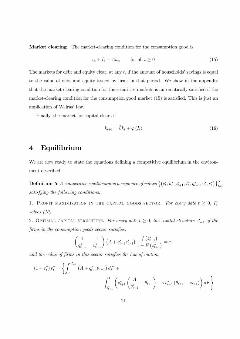
Market clearing The market-clearing condition for the consumption good is

+ = for all ≥ 0 (15)

The markets for debt and equity clear, at any , if the amount of households’ savings is equal

to the value of debt and equity issued by firms in that period. We show in the appendix

that the market-clearing condition for the securities markets is automatically satisfied if the

market-clearing condition for the consumption good market (15) is satisfied. This is just an

application of Walras’ law.

Finally, the market for capital clears if

+1 = + () (16)

4 Equilibrium

We are now ready to state the equations defining a competitive equilibrium in the environ-

ment described.

Definition 5 A competitive equilibrium is a sequence of values©¡∗

∗

∗+1

∗

∗+1

∗

∗

¢ª∞=0

satisfying the following conditions:

1. Profit maximization in the capital goods sector. For every date ≥ 0, ∗

solves (10).

2. Optimal capital structure. For every date ≥ 0, the capital structure ∗+1 of thefirms in the consumption goods sector satisfies:µ

1

∗+1− 1

∗+1

¶¡+ ∗+1

∗+1

¢ ¡∗+1

¢1−

¡∗+1

¢ =

and the value of firms in this sector satisfies the law of motion

(1 + ∗ ) ∗ =

½Z ∗+1

0

¡+ ∗+1+1

¢ +Z 1

∗+1

µ∗+1

µ

∗+1+ +1

¶− ∗+1 (+1 − +1)

¶

)

21

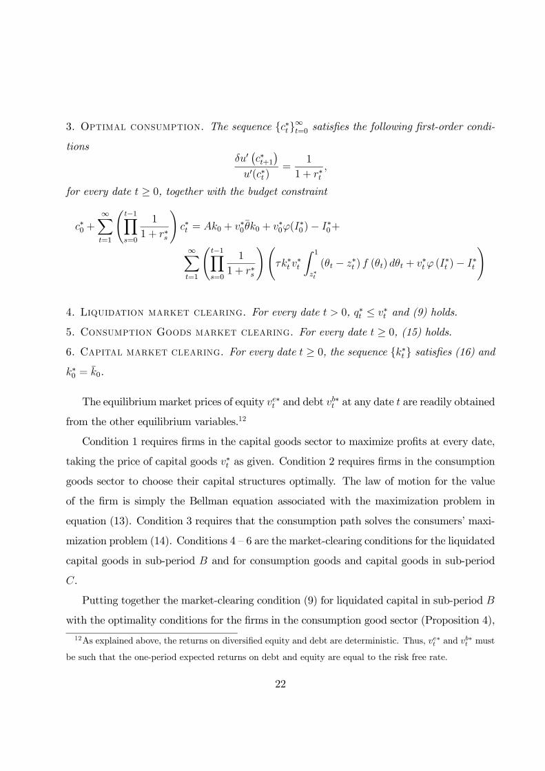
3. Optimal consumption. The sequence {∗}∞=0 satisfies the following first-order condi-tions

0¡∗+1

¢0(∗ )

=1

1 + ∗

for every date ≥ 0, together with the budget constraint

∗0 +∞X=1

Ã−1Y=0

1

1 + ∗

!∗ = 0 + ∗0 0 + ∗0(

∗0 )− ∗0+

∞X=1

Ã−1Y=0

1

1 + ∗

!Ã∗

∗

Z 1

∗

( − ∗ ) () + ∗ (∗ )− ∗

!

4. Liquidation market clearing. For every date 0, ∗ ≤ ∗ and (9) holds.

5. Consumption Goods market clearing. For every date ≥ 0, (15) holds.6. Capital market clearing. For every date ≥ 0, the sequence {∗ } satisfies (16) and∗0 = 0.

The equilibriummarket prices of equity ∗ and debt ∗ at any date are readily obtained

from the other equilibrium variables.12

Condition 1 requires firms in the capital goods sector to maximize profits at every date,

taking the price of capital goods ∗ as given. Condition 2 requires firms in the consumption

goods sector to choose their capital structures optimally. The law of motion for the value

of the firm is simply the Bellman equation associated with the maximization problem in

equation (13). Condition 3 requires that the consumption path solves the consumers’ maxi-

mization problem (14). Conditions 4 — 6 are the market-clearing conditions for the liquidated

capital goods in sub-period and for consumption goods and capital goods in sub-period

.

Putting together the market-clearing condition (9) for liquidated capital in sub-period

with the optimality conditions for the firms in the consumption good sector (Proposition 4),

12As explained above, the returns on diversified equity and debt are deterministic. Thus, ∗ and ∗ must

be such that the one-period expected returns on debt and equity are equal to the risk free rate.

22

we see that in equilibrium we must have an interior optimum for the firms’ capital structure:

∈ (0 1), and .13 Thus, default is costly and occurs with probability strictly between

zero and one:

0 () 1

Intuitively, if default were costless ( = ) firms would choose 100% debt financing, but this

implies default with probability one, which is inconsistent with market clearing. Similarly,

100% equity financing implies that there is no default and hence default is costless, so firms

should use 100% debt financing instead. The only remaining alternative is a mixture of debt

and equity and costly default.

We also see from the previous analysis that uncertainty only affects the returns and

default decisions of individual firms. All other equilibrium variables, aggregate consumption,

investment, and market prices are deterministic.

4.1 Steady-state equilibria

A steady state is a competitive equilibrium {(∗ ∗ ∗ ∗ ∗ ∗ ∗ )}∞=0 in which for all ≥ 0

(∗ ∗

∗

∗

∗

∗

∗ ) = (

∗ ∗ ∗ ∗ ∗ ∗ ∗)

We show first that a steady state exists and is unique. In addition, the system of condi-

tions defining a steady state can be reduced to a system of two equations.

Proposition 6 Under the maintained assumptions, there exists a unique steady-state equi-

librium, obtained as a solution of the following system of equations:

∗ =(1− (∗))R ∗0

() (17)

∗ =

1− + R 1∗( − ∗)

1− (18)µ

1

∗− 1

∗

¶(+ ∗∗)

(∗)1− (∗)

= (19)

13Condition 2 above is in fact stated for this case.

23

We can then also identify some of the comparative statics properties of the steady state.

Proposition 7 (i) An increase in the tax rate increases the steady value of ∗ (and hence

the debt-equity ratio) and reduces the one of ∗, but the effect on ∗ (and hence ∗ and ∗)

is ambiguous.

(ii) An increase in the discount factor decreases the steady-state value of ∗ (and hence the

debt-equity ratio) and increases the one of ∗ as well of ∗, so that ∗ and ∗ increase too.

To get some intuition for these results, consider in particular the case of an increase in

the tax rate . This increases the cost of equity financing, so that firms shift to higher debt

financing, thus decreasing the liquidity available in sub-period B and hence the liquidation

value of defaulting firms. While the direct effect of the higher tax rate, by making equity

financing costlier, is clearly to decrease , the fact that the higher tax increases debt financing

() has an opposite effect on , increasing it as we see from (18), hence the ambiguity of the

overall effect on .

4.2 Transition dynamics

The steady state is often studied because of its simplicity, but non-steady-state paths may

have very different properties. For this particular model, however, the steady state is repre-

sentative of equilibrium paths in general, at least if one is willing to assume a linear utility

function.14 In that case, we can show that, in any equilibrium, there is a constant equilib-

rium capital structure which coincides with the steady state capital structure; the same is

then true for and . Thus, outside the steady state, the only variable that is changing

is the capital stock, which converges monotonically to the steady-state value. In this sense,

little is lost by focusing on the steady state. The analysis of transition dynamics is relegated

for completeness to Appendix B.

14Since there is no aggregate uncertainty, risk aversion is not an issue. The only role played by the

curvature of the utility function is to determine the intertemporal marginal rate of substitution (IMRS).

By assuming that the utility function is linear, one imposes a constant IMRS. This restricts somewhat the

adjustment of endogenous variables along the transition path, but is otherwise innocuous.

24

5 Welfare analysis

5.1 The inefficiency of equilibrium

If we compare the conditions for a Pareto efficient steady state derived in Proposition 2 with

the conditions for a steady-state equilibrium derived in Section 4.1, we find that steady-state

equilibria are Pareto efficient if ∗ = , which happens when the equilibrium market value

of capital is given by

∗ =

1−

From the equilibrium conditions, in particular Condition 2, it can be seen immediately that

the equality above can hold only if = 0. In that case, there is no cost of issuing equity and

the firms in the consumption goods sector will choose 100% equity finance. On the other

hand, when 0, as we have been assuming, the equilibrium market value of capital ∗ is

strictly lower than 1− and

∗ and ∗ are strictly less than the corresponding values at the

first best steady state. Thus, in a steady state equilibrium, the financial frictions given by

market incompleteness and the costs of default and equity financing as perceived by firms

imply that firms invest a lower amount and the equilibrium stock of capital is lower than at

the efficient steady state. Hence even with a representative consumer, competitive equilibria

are Pareto inefficient15.

Short of getting rid of the corporate income tax, a policy of reducing the tax rate across

the board would also improve welfare. As we saw in the comparative statics exercise, a

reduction in the tax rate will increase the value of the firm (capital goods), causing an

increase in investment and consumption. Similarly, policies such as accelerated depreciation,

expensing of investments in research and development, or subsidies on investment, which

have the effect of reducing the effective tax rate will also increase welfare.

15When the initial capital stock 0 = the unique Pareto efficient allocation of the economy is the

Pareto efficient steady state. Since as we saw the equilibrium allocation is different, it is clearly Pareto

inefficient. For other values of 0 the transitional dynamics of the Pareto efficient allocation needs also to

be considered to claim the inefficiency of the equilibrium. This can be shown formally by proceeding along

similar lines to the ones of the next section.

25

In our simplified model, all firms are ex ante identical, so the most effective policy is a

uniform reduction of the tax rate. If firms are heterogeneous, however, it might be advan-

tageous to target firms that are vulnerable to fire sales, either because they are riskier or

because they have less liquid markets for liquidated capital goods. In that case, a uniform

tax rate on corporate income, combined with incentives for particular industries, might be

called for.

5.2 Constrained inefficiency

It is not surprising that the equilibrium is Pareto-inefficient in the presence of financial

frictions affecting firms’ financing. To assess the scope of policy and regulatory interventions,

however, it is more interesting and appropriate to see whether a welfare improvement can

be found, taking as given the presence of such frictions (market incompleteness, liquidity

constraints and distortionary taxation). More precisely, we examine whether regulating the

levels of a single endogenous variable, in particular, the capital structure as represented

by , can lead to a welfare improvement while allowing all other variables to reach their

equilibrium levels. If so, we say that competitive equilibria are constrained inefficient.

Suppose the economy is in a steady state equilibrium and consider an intervention con-

sisting in a permanent16 change ∆ starting at some fixed but arbitrary date + 1. Thus

from this date onwards is constant and equal to ∗+∆ To determine the welfare effects

of this intervention we need to trace the changes in equilibrium prices, investment and con-

sumption over time and hence the transition to the new steady state. To make this analysis

more transparent, we assume consumers are risk neutral17, that is, () = .

The induced changes in the equilibrium variables and are then obtained by substi-

tuting the new value of into the market-clearing condition in sub-period , (9),

(1− (∗ +∆)) = +1+

Z ∗+∆

0

(20)

16We focus attention on a permanent intervention, but it is fairly easy to verify that the same welfare

result holds in the case of a temporary intervention.17See footnote 14 for a discussion of this specification of consumers’ preferences.

26

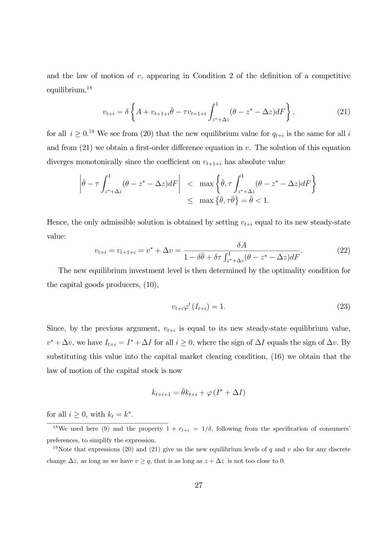
and the law of motion of , appearing in Condition 2 of the definition of a competitive

equilibrium,18

+ =

½+ +1+ − +1+

Z 1

∗+∆

( − ∗ −∆)

¾ (21)

for all ≥ 019 We see from (20) that the new equilibrium value for + is the same for all and from (21) we obtain a first-order difference equation in . The solution of this equation

diverges monotonically since the coefficient on +1+ has absolute value¯ −

Z 1

∗+∆

( − ∗ −∆)

¯ max

½

Z 1

∗+∆

( − ∗ −∆)

¾≤ max

©

ª= 1

Hence, the only admissible solution is obtained by setting + equal to its new steady-state

value:

+ = +1+ = ∗ +∆ =

1− + R 1∗+∆

( − ∗ −∆) (22)

The new equilibrium investment level is then determined by the optimality condition for

the capital goods producers, (10),

+0 (+) = 1 (23)

Since, by the previous argument, + is equal to its new steady-state equilibrium value,

∗+∆, we have + = ∗+∆ for all ≥ 0, where the sign of ∆ equals the sign of ∆ By

substituting this value into the capital market clearing condition, (16) we obtain that the

law of motion of the capital stock is now

++1 = + + (∗ +∆)

for all ≥ 0, with = ∗

18We used here (9) and the property 1 + + = 1 following from the specification of consumers’

preferences, to simplify the expression.19Note that expressions (20) and (21) give us the new equilibrium levels of and also for any discrete

change ∆, as long as we have ≥ , that is as long as +∆ is not too close to 0

27

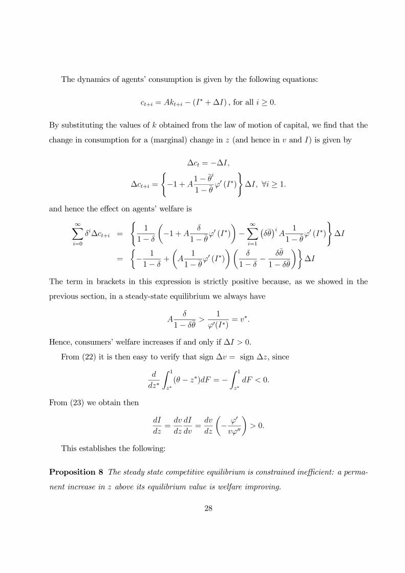
The dynamics of agents’ consumption is given by the following equations:

+ = + − (∗ +∆) , for all ≥ 0

By substituting the values of obtained from the law of motion of capital, we find that the

change in consumption for a (marginal) change in (and hence in and ) is given by

∆ = −∆

∆+ =

(−1 +

1−

1− 0 (∗)

)∆ ∀ ≥ 1

and hence the effect on agents’ welfare is

∞X=0

∆+ =

(1

1−

µ−1 +

1− 0 (∗)

¶−

∞X=1

¡¢

1

1− 0 (∗)

)∆

=

½− 1

1− +

µ

1

1− 0 (∗)

¶µ

1− −

1−

¶¾∆

The term in brackets in this expression is strictly positive because, as we showed in the

previous section, in a steady-state equilibrium we always have

1−

1

0(∗)= ∗

Hence, consumers’ welfare increases if and only if ∆ 0.

From (22) it is then easy to verify that sign ∆ = sign ∆, since

∗

Z 1

∗( − ∗) = −

Z 1

∗ 0

From (23) we obtain then

=

=

µ− 0

00

¶ 0

This establishes the following:

Proposition 8 The steady state competitive equilibrium is constrained inefficient: a perma-

nent increase in above its equilibrium value is welfare improving.

28

The intervention is specified in terms of the threshold below which the firm has to

default on its debt. It can be easily verified that a marginal increase of this threshold above

∗ corresponds to an increase in the firms’ debt-equity ratio. The ratio between the market

value of the firm’s debt and that of its equity is in fact given by20

++

=

R 0(+ +1+) +

R 1+1+

³

+1++ ´R 1

+1+( − ) (1− )

(24)

The denominator is clearly decreasing in . Since + + + = + and ∗ maximizes the

firms’ market value + the numerator must increase with , and so ++.

Proposition 8 establishes the optimality of a marginal increase in Consider then a

sequence of discrete changes ∆, such that + ∆ approaches 1. Along such a sequence,

goes to zero21 and we also see from (22) that approaches 1− and hence, by (6),

approaches . That is, in the limit, the equilibrium corresponding to such an intervention

converges to the steady-state, first-best allocation.22 We can then say that the constrained

optimal capital structure of firms exhibit maximal leverage.

To get some understanding of the determinants of the above result, note first that, when

firms increase their leverage, that is, is increased above ∗, the tax paid on each unit of

capital, R 1(−) , decreases. At the same time, as we can see from the expression of the

firms’ market value in (13), firms face a higher probability and hence a higher expected cost

of default, given by the difference between the liquidated value of the firm’s assets, , and

the normal market value, . At a competitive equilibrium, firms do not want to deviate from

∗ as the benefits and costs of a marginal increase in leverage offset each other. The cost of

default depends, however, on prices and, when all firms change their leverage choices, prices

20The term on the denominator, is obtained from the expression of the pre-tax value of the equity of the

firm, when solvent, obtained in (11). This is then subtracted from the overall value of the firm, in (13), to

obtain the value of debt.21Note that the equilibrium condition (20) has an admissible solution for all +∆ 1, but not in the

limit for +∆ = 122In contrast, we see from (12), that when firms act as price takers their optimal decision when → 0 is

∼ 0

29

change. Once we substitute for its equilibrium value from the market-clearing condition

(9), as we did in (22), we find that the higher losses incurred by a firm when bankrupt are

perfectly offset by the higher gains made when solvent (when the firm is able to buy capital

at cheaper prices). As a consequence, the net effect of an increase in by all firms, when we

take the change in prices into account, is just the decrease in the cost of the tax paid, and the

firms’ value increases. Thus, once the pecuniary externality is internalized, the cost of debt

financing turns out to be lower than the cost perceived by firms. Hence, a higher leverage

induces a higher level of . This in turn increases the firms’ investment, which raises the

capital stock in the economy. Since the equilibrium accumulation of capital is inefficiently

low, as we noticed in Section 5.1, due to costs of equity and debt financing perceived by

firms, the increase in investment and capital generates a welfare improvement.

The cost of bankruptcy as perceived by firms is a pure transfer, as the fire sale losses of

bankrupt firms provide capital gains for the solvent firms. The same is true for the corporate

income tax, in that case a transfer from solvent firms to consumers. Since the tax revenue is

paid directly to households, one might think this has something to do with the fact that the

tax reduces . In fact, it depends crucially on how the tax revenues are paid out. Suppose

the revenues from the tax were paid to firms instead of households. The distortion will

remain as long as the transfers are lump sum, i.e., not proportional to the firm’s capital

stock. A rational manager will perceive that an increase in the firm’s capital stock increases

its tax liability, but does not increase the transfer received, so he will still have an incentive

to underinvest in equilibrium. Only if the transfer were proportional to the value of equity,

i.e., the tax base, would the distortionary effect disappear.

It is important to note that our result on the welfare benefits of increasing firms’ leverage

does not depend on the absence of deadweight costs of bankruptcy. Suppose we were to

assume that bankrupt firms lose a fraction 0 1 of their output, consumed by the

costs of the bankruptcy process. Each firm would take into account this additional cost of

bankruptcy when it chooses its optimal capital structure. The actual costs of bankruptcy for

the firm (the costs once the pecuniary externality is internalized) in this case are positive,

30

but it is still true that they are lower than the costs privately perceived by the firm, since the

latter overestimate the costs of fire sales, due to the pecuniary externality. As a consequence,

it remains true that increasing ∗ will increase the value of capital ∗ and as a result the level

of investment and the capital stock will increase too. Since the equilibrium again exhibits

underinvestment, such increase in the investment level always increases welfare, as in the

situation considered in this section.

But now an increase in ∗ has another effect on welfare, going in the opposite direction,

as it will also increase the deadweight costs of bankruptcy and hence reduce the resources

that a given stock of capital generates for consumption. Which of the two effects dominates

depends on the elasticity of investment with respect to ∗ and hence ∗. In Appendix B

we replicate the analysis for the economy with deadweight costs of bankruptcy and show

that, if the elasticity of investment with respect to ∗ is sufficiently high, an increase in

∗ is welfare-improving.since the increase in investment is sufficiently large relative to the

increase in deadweight costs. Thus, the distortion caused by fire sales remains the crucial

determinant of the welfare effects of an increase in firms’ leverage.

6 Conclusion

We have analyzed the firms’ capital structure choice in a dynamic general equilibrium econ-

omy with incomplete markets. Firms face a standard trade-off between the exemption of

interest payments on debt from the corporate income tax and the risk of costly default. The

latter cost arises from the fact that a firm defaulting on its debt may be forced to liquidate

its assets in a fire sale. Fire sales are endogenously determined in equilibrium and arise from

the illiquidity of the capital market where the firm’s assets are sold. When the corporate

income tax rate is positive we show that fire sales are an essential part of the equilibrium,

the optimal capital structure is uniquely determined in equilibrium and firms’ investment is

lower than at its first-best level. Moreover, the debt/equity ratio chosen by firms is ineffi-

ciently low: a regulatory intervention inducing firms to increase their leverage generates an

31

increase of firms’ return to capital and hence also of their investment level and of consumers’

welfare.

These findings highlight the importance of recognizing the presence of a pecuniary exter-

nality when evaluating the cost of default due to fire sales. The sale of the assets of bankrupt

firms at fire-sale prices clearly entails a loss for such firms, but constitutes at the same time

a gain for solvent firms who are so able to purchase capital cheaply. Our analysis shows

that, by ignoring the effect of a higher leverage ratio on the fire-sale price of firms’ assets,

firms underestimate the benefits of these purchases and perceive the cost of debt as higher

than what it actually is. It is through such pecuniary externalities, concerning the price of

liquidated assets, that interventions modifying the firms’ capital structure affect welfare in

general equilibrium when markets are incomplete.

We also showed the robustness of our findings to the presence of additional, deadweight

costs of firms’ default given by the destruction of value of the firms’ assets. As long as

firms perceive the negative effect of these deadweight costs on their market value, they will

still overestimate the costs of debt financing and hence an intervention increasing firms’

leverage still increases investment. We can also think however at environments where there

are deadweight costs of bankruptcy that firms do not take into account, for instance costs

imposed on other firms because of the disruption in the financial system23, in which case

a higher leverage may have detrimental effects on firms’ investments. In any case, as we

noticed, in the presence of deadweight costs of bankruptcy higher leverage also means higher

social costs in terms of the destruction of resources produced by bankruptcy, so we have

forces pulling in opposite directions the constrained efficient level of firms’ leverage relative

to the equilibrium one, but the effect we identified remains present.

Although the model we have studied deals with corporate debt, the results are suggestive

for the current debate about the funding and capital structure of financial institutions in the

23Also, in Lorenzoni (2008) and some of the other papers mentioned in the Introduction the capital of

bankrupt firms can only be sold to different types of firms who operate a less productive technology, hence

there is a deadweight cost attached to fire sales.

32

wake of the financial crisis. A similar exercise for financial institutions would seem to be an

important topic for future research.

In the rest of this section, we briefly discuss the sensitivity of our results to some of the

features of the model.

Aggregate uncertainty A special feature of our model is the fact that the shocks af-

fecting firms are purely idiosyncratic and there is no aggregate risk. There has been a lot

of interest in the macroeconomic literature about the role of financial frictions in the prop-

agation of economic shocks. A large and influential stream of this literature concerns the

financial accelerator. In this literature, recalled in the Introduction, firms’ financing plays

an important role. Because of moral hazard problems, firms’ ability to borrow is limited by

the value of equity or of the assets that serve as collateral. A negative shock to the value

of equity and collateral reduces the firms’ ability to borrow for investment and this in turn

propagates through the cycle. In recent papers (Gertler and Kiyotaki, 2010), the focus has

been shifted to the role of banks and the way in which fluctuations in bank capital restrict

lending and propagate business cycle disturbances.

Our focus, unlike this macroeconomic literature, is on questions of efficiency and regu-

lation, rather than business cycle dynamics. Extending the analysis to include aggregate

uncertainty would make the model less tractable, but we believe it would not change the

fundamental qualitative features of the results we obtained. Suppose, for example, that we

introduce an additional, aggregate shock affecting the depreciation of firms’ capital: each

unit of capital used by firm at date is reduced, after production of the consumption good,

to units, where is a common shock and and are independent.24 The law of

motion of capital becomes

+1 = + ()

hence the accumulation of capital is now stochastic.

In this simple environment, under suitable conditions on agents’ preferences, both the

24See Appendix B for a formal analysis of this case and the derivation of some properties of equilibria.

33

equilibrium value of liquidated capital and the market value of capital decrease with the

magnitude of the shock while the firms’ capital structure, as described by , is not affected

by . Also, the pecuniary externality is still present, leading firms to overestimate the cost of

bankruptcy and debt financing and implying that there is too much debt in the equilibrium

capital structure.

More generally, the extension of the model to allow for aggregate risk could offer some

interesting implications for the properties of the equilibrium prices of debt and equity, as

well as for the pattern of consumption and investment over the business cycle. The effects

of aggregate uncertainty on the firms’ choice of capital structure is also of interest. We plan

to pursue these issues in future work.

Liquidity provision In our stylized model, there is only one technology for producing

consumption goods. The only choice for the firms in the consumption goods sector is how

to finance their purchases of capital goods. In particular, they have no control over the

riskiness of the production technology. This may be seen as a limitation, since in practice

firms may be able to diversify their business lines to reduce the risk of default. To test the

robustness of our results, it is then useful to consider an extension of the analysis where an

alternative, safe technology can be used to produce consumption goods using capital goods.

The safe technology is subject to a non-stochastic depreciation rate 1 − , but has a lower

productivity .

We can interpret the safe technology as a way to provide liquidity in the economy. It

allows firms to make capital gains from the purchase of assets in fire sales whenever liquidity

is scarce in the system. It can be shown25 that in equilibrium firms will specialize in one of

the technologies. There proves to be in fact no advantage to combining the safe and risky

technology. More interestingly, we find that introducing the safe technology does little to

mitigate the inefficiency: on the contrary it generates an additional source of inefficiency

and, as long as is not too high, it reduces welfare. Although the presence of firms using

25The details are in Appendix B.

34

the safe technology reduces the scale of the fire sales and raises the price of liquidated

assets, it reduces the returns to capital and hence the incentives to invest. The mechanism

generating the inefficiency is now partly different: the introduction of a safe technology

diverts the capital gains from purchases at fire-sale prices to the firms choosing the safe but

less productive technology, thus depriving the firms choosing the risky technology of some

of those gains.

References

[1] Aghion, Philippe, Oliver Hart, and John H. Moore (1992). “The Economics of Bank-

ruptcy Reform,” Journal of Law, Economics and Organization 8, 523-546.

[2] Allen, F. and D. Gale (2004a). “Financial Intermediaries and Markets,” Econometrica

72, 1023-1061.

[3] Allen, F. and D. Gale (2004b). “Financial Fragility, Liquidity, and Asset Prices” Journal

of the European Economic Association 2, 1015-1048.

[4] Arnott, Richard and J.E. Stiglitz (1986). “Moral hazard and optimal commodity taxa-

tion,” Journal of Public Economics 29, l-24.

[5] Barnea, Amir, Robert A. Haugen and LemmaW. Senbet (1981) “An EquilibriumAnaly-

sis of Debt Financing Under Costly Tax Arbitrage and Agency Problems,” The Journal

of Finance 36, 569-581.

[6] Bebchuk, Lucian A. (1988). “A New Approach to Corporate Reorganizations,” Harvard

Law Review 101, 775-804.

[7] Bernanke, B.S. and M. Gertler (1989). “Agency costs, net worth, and business fluctua-

tions,” American Economic Review 79, 14—31

35

[8] Bernanke, B.S., Mark Gertler, and Simon Gilchrist (1999). “The financial accelerator

in a quantitative business cycle framework,” Chapter 21 Handbook of Macroeconomics,

Volume 1, Part C, 1341—1393.

[9] Bianchi, Javier (2011). “Overborrowing and Systemic Externalities in the Business Cy-

cle,” American Economic Review, 101 (7), 3400-26.

[10] Bolton, Patrick, Hui Chen and Neng Wang (2011). “A Unified Theory of Tobin’s ,

Corporate Investment, Financing, and Risk Management,” forthcoming in The Journal

of Finance.

[11] Bradley, Michael, Gregg A. Jarrell and E. Han Kim (1984) “On the Existence of an

Optimal Capital Structure: Theory and Evidence,” The Journal of Finance 39, 857-

878.

[12] Brennan, M. J. and E. S. Schwartz (1978) “Corporate Income Taxes, Valuation, and

the Problem of Optimal Capital Structure,” The Journal of Business 51, 103-114.

[13] Dammon, Robert M. and Richard C. Green (1987) “Tax Arbitrage and the Existence

of Equilibrium Prices for Financial Assets,” The Journal of Finance 42, 1143-1166.

[14] Eberly, Janet, Sergio Rebelo and Nicolas Vincent (2008) “Investment and Value: A

Neoclassical Benchmark,” NBER Working Paper No. 13866.

[15] Fischer, Edwin O., Robert Heinkel and Josef Zechner (1989) “Dynamic Capital Struc-

ture Choice: Theory and Tests,” The Journal of Finance 44, 19-40.

[16] Gale, D. and P. Gottardi (2011). “Bankruptcy, Finance Constraints and the Value of

the Firm,” American Economic Journal: Micro 3, 1-31.

[17] Geanakoplos, J. and H. Polemarchakis (1986). "Existence, Regularity, and Constrained

Suboptimality of Competitive Allocations When the Asset Market Is Incomplete," in

Walter, Heller, Ross Starr, and David Starrett eds. Essays in honor of Kenneth J. Arrow:

36

Volume 3, Uncertainty, Information and Communication. Cambridge, New York and

Sydney: Cambridge University Press, 65-95.

[18] Gersbach, Hans and Jean-Charles Rochet (2012). “Aggregate Investment Externalities

and Macroprudential Regulation,” Journal of Money, Credit and Banking 44, 73—109.

[19] Gertler, Mark and Nobuhiro Kiyotaki (2010). “Financial Intermediation and Credit

Policy in Business Cycle Analysis,” Handbook of Monetary Economics Volume 3A, ed.

B.M. Friedman and M. Woodford, North-Holland).

[20] Gomes, João and Lukas Schmid (2010). “Equilibrium Credit Spreads and

the Macroeconomy,” AFA 2010 Atlanta Meetings Paper. Available at SSRN:

http://ssrn.com/abstract=1363840.

[21] Greenwald, Bruce C. and Joseph E. Stiglitz (1986). “Externalities in Economies with

Imperfect Information and Incomplete Markets,” The Quarterly Journal of Economics

101, 229-264.

[22] Hackbarth, Dirk and David C. Mauer (2012).“Optimal Priority Structure, Capital

Structure, and Investment,” Review of Financial Studies 25, 747-796.

[23] Hart, Oliver D. (1979) “On Shareholder Unanimity in Large Stock Market Economies,”

Econometrica 47, 1057-1083.

[24] Kim, E. Han (1982) “Miller’s Equilibrium, Shareholder Leverage Clienteles, and Opti-

mal Capital Structure,” The Journal of Finance 37, 301-319.

[25] Kiyotaki, Nobuhiro and John Moore (1997). “Credit Cycles,” Journal of Political Econ-

omy, 105, 211-248.

[26] Korinek, Anton (2012). “Systemic Risk-Taking: Amplification Effects, Externalities,

and Regulatory Responses” University of Maryland, manuscript.

37

[27] Kuehn, Lars-Alexander and Lukas Schmid (2014). “Investment-Based Corporate Bond

Pricing,” forthcoming in The Journal of Finance.

[28] Leland, Hayne E. and Klaus Bjerre Toft (1996) “Optimal Capital Structure, Endogenous

Bankruptcy, and the Term Structure of Credit Spreads,” The Journal of Finance 51,

987-1019.

[29] Lorenzoni, Guido (2008). “Inefficient Credit Booms,” Review of Economic Studies 75,

809-833.

[30] Miao, Jianjun and Pengfei Wang (2010). “Credit Risk and Business Cycles,” Boston

University, manuscript.

[31] Miller, Merton H. (1977) “Debt and Taxes,” The Journal of Finance 32, 261-275.

[32] Modigliani, Franco and Merton H. Miller (1958) “The Cost of Capital, Corporation

Finance and the Theory of Investment,” The American Economic Review 48, 261-297.

[33] Shleifer, Andrei and Robert W. Vishny (1992). “Liquidation Values and Debt Capacity:

A Market Equilibrium Approach,” Journal of Finance 47, 1343-1366.

[34] Sundaresan, Suresh, Neng Wang and Jinqiang Yang (2014). “Dy-

namic Investment, Capital Structure, and Debt Overhang,” available at

http://www0.gsb.columbia.edu/faculty/nwang/papers/Sundaresan_Wang_Yang_2014.pdf.

[35] Titman, S. (1984). “The effect of capital structure on a firm’s liquidation decision,”

Journal of Financial Economics 13, 137—151.

[36] Titman, Sheridan and Roberto Wessels (1988) “The Determinants of Capital Structure

Choice,” The Journal of Finance 43, 1-19.

38

Proofs

Proof of Proposition 1 From the strict concavity of and the gradient inequality, it

follows that, for any ,

() ≤ ³´+ 0

³´³ −

´=

¡1−

¢ + 0

³´³ −

´

¡1−

¢

Hence

() + ¡1−

¢ +

For any ,

() ≤ ³´+ 0

³´³ −

´

¡1−

¢ +

¡1−

¢ ³ −

´=

¡1−

¢

where the second inequality follows from the assumptions made on (·), implying the exis-tence of a unique solution for . Thus,

=⇒ +1

and

=⇒ +1

Proof of Proposition 2 At an optimal steady state the multipliers {(∗ ∗ )}∞=0 satisfy

∗ = 0 (∗) = ∗0

and hence

∗ =∗

0 (∗)=

∗0∗0

∗0

= ∗0

39

for every . The first-order conditions for the steady-state optimum can then be written as

0 (∗) = ∗0 (25)

∗0+ ∗0 = ∗0 (26)

∗00 (∗) = ∗0 (27)

Conditions (26) and (27) can be rewritten as

1− =

∗0∗0=

1

0 (∗)(28)

The feasibility conditions become

∗ + ∗ = ∗

and

∗ = ∗ + (∗)

Thus,

∗ = (∗)1−

where ∗ is determined by (28).

Proof of Proposition 4 The derivative of the expression in (13) with respect to +1 is

easily calculated to be

1

1 +

½(+ +1+1) (+1)− +1

µ

+1+ +1

¶ (+1) +

+1 (+1 − +1) (+1) + +1 (1− (+1))}

=1

1 +

½µ1− +1

+1

¶ (+1) +

µ1− +1

+1

¶+1+1 (+1) + +1 (1− (+1))

¾

The first-order condition for an interior solution of the firm’s problem requires this expression

to equal zero, a condition which can be written asµ+1

+1− 1¶(+ +1+1) (+1) = +1 (1− (+1))

40

or µ1

+1− 1

+1

¶(+ +1+1)

(+1)

1− (+1)=

A solution to this equation, if it exists, is unique since all terms on the left hand side are

positive and increasing in +1. The term + +1+1 is in fact clearly increasing in +1,

and so is(+1)

1− (+1) under the assumption of an increasing hazard rate.

From the above expression we then see that when³

1+1− 1

+1

´ (0) ≥ we have a

corner solution with +1 = 0. In contrast, when³

1+1− 1

+1

´ (0) (and +1 +1)

it is easy to verify that a corner solution with +1 = 1 never exists. By the continuity of

the objective function in +1, a solution always exists, so it follows that an interior solution

exists.

Market clearing in the securities market The value of debt and equity issued by each

firm at any is equal to the market value of depreciated capital, , plus the value of

newly produced capital goods, () To find the consumer’s savings, we need first to find

the value of the consumer’s wealth in sub-period of date . This is equal to the sum of

the profits from the capital good sector, the proceeds from the liquidation of firms which

defaulted in this period, and the value of the firms that did not default in the period minus

the corporation tax plus the lump sum transfer from the government. The corporation tax

and the transfer cancel in equilibrium, hence the consumer’s wealth, , is given by

= ()− +

Z

0

(+ ) +

Z 1

µ

+

¶

Using the market clearing condition in the liquidation market (9), this simplifies to:

= ()− + +

Therefore, the securities market clears at date if

− = ()− + + −

= ¡ + ()

¢41

or

+ =

So market clearing in the consumption good market (15) implies market clearing in the

securities markets, as claimed.

Proof of Proposition 6 Equations (17) and (19) come directly from Conditions 4 and 2

of the definition of competitive equilibrium, applied to a steady state. From the equation

specifying the law of motion of the value of the firm, using the fact that at a steady state

1(1 + ∗) = , we then get

∗ =

½Z ∗

0

(+ ∗) +Z 1

∗

µ∗

∗(+ ∗)− ∗( − ∗)

¶

¾=

½Z ∗

0

µ+ ∗ −

µ∗

∗− 1¶∗

¶ +

Z 1

∗

µ+ ∗ +

µ∗

∗− 1¶− ∗( − ∗)

¶

¾=

½+ ∗ −

Z 1

∗( − ∗)

¾where in the last step we used (17) to simplify the expression. Solving for we get:

∗ =

1− + R 1∗ ( − ∗)

that is, equation (18).

Let (∗) denote the solution of equation (18) with respect to and (∗) that of (17),

also with respect to Note that (∗) is a strictly increasing and (∗) a strictly decreasing

function of ∗. The remaining condition (19) can then be written asµ1− (∗)

(∗)

¶µ

(∗)+ ∗

¶ (∗)

1− (∗)= (29)

and it is clear from inspection that all the terms on the left hand side are increasing in ∗,

so there exists at most one solution, that is one steady state.

To see that there exists a solution to (29), note that as ∗ → 0, (∗) → ∞ and

(∗) → 1−+ , so for some finite value

∗ 0 we have (∗) = (∗) and the left hand

side of (29) equals zero. Next, consider what happens as ∗ → 1 and note that (∗) → 0

and (∗) → 1− 0, so the left hand side of (29) is positive and arbitrarily large. Thus,

by continuity, there exists a value of 0 ∗ 1 satisfying (29).

42

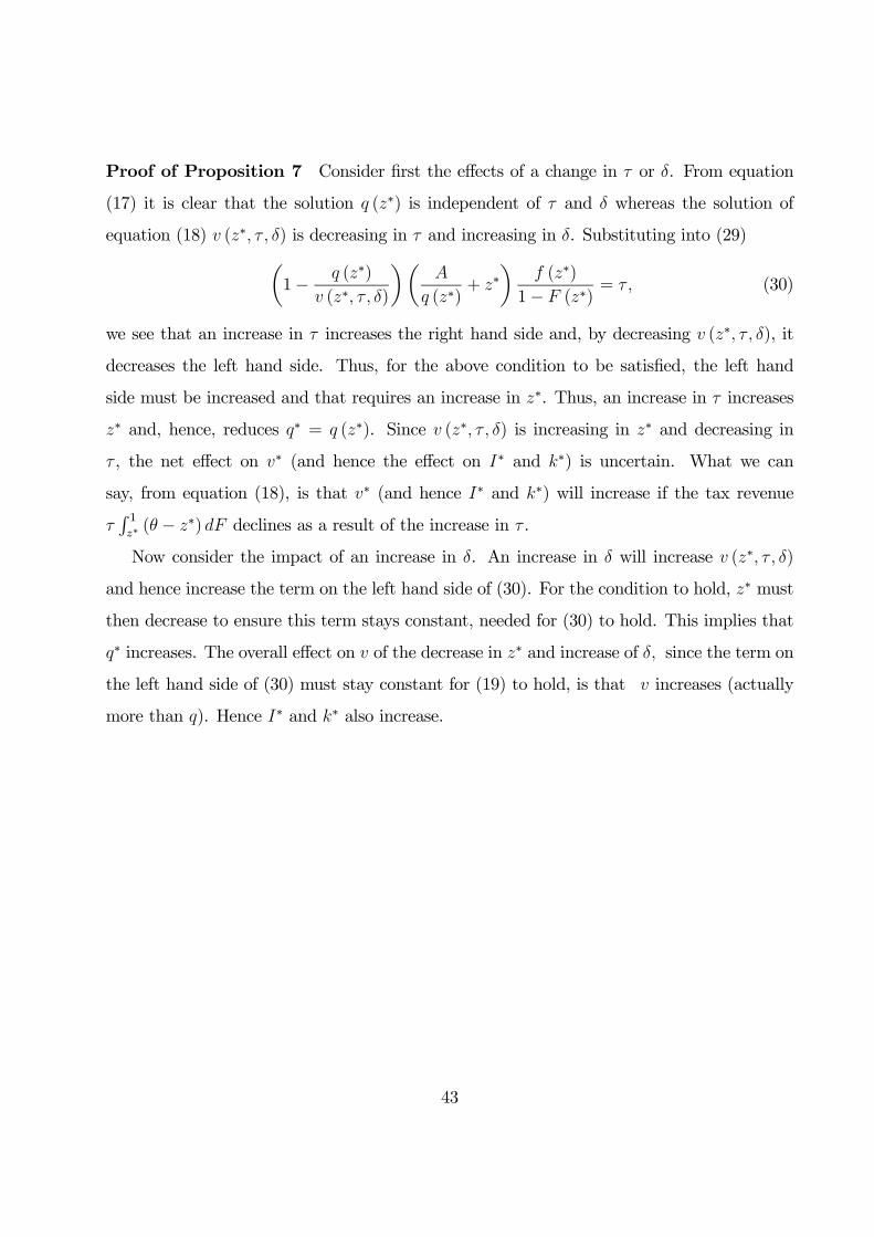
Proof of Proposition 7 Consider first the effects of a change in or . From equation

(17) it is clear that the solution (∗) is independent of and whereas the solution of

equation (18) (∗ ) is decreasing in and increasing in . Substituting into (29)µ1− (∗)

(∗ )

¶µ

(∗)+ ∗

¶ (∗)

1− (∗)= (30)

we see that an increase in increases the right hand side and, by decreasing (∗ ), it

decreases the left hand side. Thus, for the above condition to be satisfied, the left hand

side must be increased and that requires an increase in ∗. Thus, an increase in increases

∗ and, hence, reduces ∗ = (∗). Since (∗ ) is increasing in ∗ and decreasing in

, the net effect on ∗ (and hence the effect on ∗ and ∗) is uncertain. What we can

say, from equation (18), is that ∗ (and hence ∗ and ∗) will increase if the tax revenue

R 1∗ ( − ∗) declines as a result of the increase in .

Now consider the impact of an increase in . An increase in will increase (∗ )

and hence increase the term on the left hand side of (30). For the condition to hold, ∗ must

then decrease to ensure this term stays constant, needed for (30) to hold. This implies that

∗ increases. The overall effect on of the decrease in ∗ and increase of since the term on

the left hand side of (30) must stay constant for (19) to hold, is that increases (actually

more than ). Hence ∗ and ∗ also increase.

43

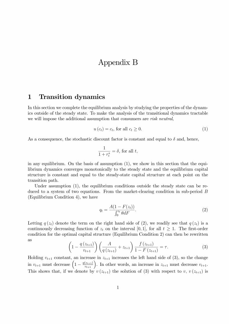
Appendix B

1 Transition dynamics

In this section we complete the equilibrium analysis by studying the properties of the dynam-

ics outside of the steady state. To make the analysis of the transitional dynamics tractable

we will impose the additional assumption that consumers are risk neutral,

() = , for all ≥ 0 (1)

As a consequence, the stochastic discount factor is constant and equal to and, hence,

1

1 + ∗= , for all

in any equilibrium. On the basis of assumption (1), we show in this section that the equi-

librium dynamics converges monotonically to the steady state and the equilibrium capital

structure is constant and equal to the steady-state capital structure at each point on the

transition path.

Under assumption (1), the equilibrium conditions outside the steady state can be re-

duced to a system of two equations. From the market-clearing condition in sub-period

(Equilibrium Condition 4), we have

=(1− ())R

0

(2)

Letting () denote the term on the right hand side of (2), we readily see that () is a

continuously decreasing function of on the interval [0 1], for all ≥ 1. The first-order

condition for the optimal capital structure (Equilibrium Condition 2) can then be rewritten

as µ1− (+1)

+1

¶µ

(+1)+ +1

¶ (+1)

1− (+1)= (3)

Holding +1 constant, an increase in +1 increases the left hand side of (3), so the change

in +1 must decrease³1− (+1)

+1

´. In other words, an increase in +1 must decrease +1.

This shows that, if we denote by (+1) the solution of (3) with respect to (+1) is

1

a continuously decreasing function of on the interval [0 1], for all ≥ 1. The profit-

maximization condition of the capital good producers (Equilibrium Condition 1),

0() = 1 (4)

implies that the investment level = () is a well defined and strictly increasing function

of . Hence (()) is a well defined and decreasing function of on the interval [0 1] for

all ≥ 0.Substituting these functions for into the expressions specifying the law of motion

of the market value of the firms in the consumption goods sector (in Equilibrium Condition

2)1 and the capital market-clearing (Equilibrium Condition 6), we obtain the system of two

difference equations below in and :

() =

∙+ (+1) − (+1)

Z 1

+1

( − +1)

¸(5)

+1 = + (()) (6)

This dynamic system can be solved for the values {( )}∞=1, subject to the initial condi-tions determining2 1. This sequence defines an equilibrium trajectory corresponding to an

equilibrium as defined in Definition 5.

The first of these, Equation (5), only depends on . Hence, the dynamics for is

determined by that equation and does not depend on . We show in the sequel that the

dynamics for is as described in the following figure:

where the red line is the graph of the term on the right hand side of (5), and the blue

line is the graph of the term on the left hand side, both regarded as functions of . The

1We also used (2) to simplify the expression in (5), as we did in the proofS of Propositions 7 and 8.2The initial conditions are given by 1 = 0 + (0) with 0 determined by

h+ (1) − (1)

R 11( − 1)

i0(0) = 1 as a function of 1.

2

two curves intersect at the unique steady-state value = ∗. At that point the slope ofthe red curve is flatter than the slope of the blue curve. Also, both curves are negatively

sloped. This implies that, starting at any initial point 1 6= ∗, the trajectory {} satisfyingthe difference equation must diverge away from ∗. In fact, if 1 ∗ is monotonicallyincreasing until it reaches a value, strictly smaller than one, beyond which a solution to (5)

no longer exists.3 On the other hand, if 1 ∗ both curves diverge to infinity and thedynamics is monotonically decreasing approaching zero. This is also unfeasible, since we see

from (3), (2), (4) that when → 0, , , and hence also tend to infinity, which violate

the boundedness property established in Proposition 1.

This shows that in any competitive equilibrium we must have = ∗ for all . From thisit follows that prices and the investment level are constant along the equilibrium path, at

the levels = (∗) = ∗, = (∗) = ∗ and = (∗) = ∗, for all , while the dynamicsof the capital stock is determined by the law of motion

+1 = + (∗)

with 1 determined by the initial conditions. Then

++1 =³ +

2+ · · ·+

´ (∗) +

+1

→ (∗)1−

= ∗ as →∞

So the capital stock converges to its steady-state value. We have thus established the fol-

lowing:

Claim 1 Let {( )}∞=1 be a solution of the two-equation system (5-6) satisfying 0 = 0.

Then {( )}∞=1 is an equilibrium trajectory only if, for all ≥ 1, = ∗, where ∗ is theuniquely determined steady-state capital structure. Furthermore, converges monotonically

to its steady-state value, ∗.

Proof. In order to complete the proof of the proposition, we need to characterize the

dynamics of the two-equation system (5-6) above. We show first that, at the unique steady-

state value = ∗, the derivative of the term on the left hand side of (5), 0 (∗), is negativeand strictly smaller than the derivative of the term on the right hand side. Denoting the

term on the right hand side by (+1), with () defined by

() =

∙+ () − ()

Z 1

( − )

¸

we have

0 (∗) = 0 (∗) − 0 (∗)Z 1

( − ) + (∗) (1− (∗))

0 (∗) 0 (∗)

3If → 1, the term on the right hand side converges to and the one on the left hand side converges to

0. Thus for some finite value of there is no value of +1 that satisfies equation (5).

3

as claimed. The first inequality follows from the fact that the second and third terms on the

right hand side of the first expression are positive, the second inequality from the fact that

0 (∗) is negative and 0 1.

Since the steady state is unique, this proves that

() ≷ () as ≶ ∗

for all 0 1.

We show next that 0 () 0, for all 0 1. This is equivalent to

− 0

(1− ())

− R 1( − )

(7)

Differentiating (3) we get

0

=

⎛⎝ ³+ ´

1−

⎞⎠

+

0

Also, from (2) we get

0 =− R

0 −(1− )¡R

0

¢2

Since −0 0, a sufficient condition for (7) to hold is that

−

⎛⎝ ³+ ´

1−

⎞⎠

= −

h³20 − 1

´ ¡

1−¢− ³

+ ´

¡

1−¢i

³+ ´2 ¡

1−¢2

(1− )

− R 1( − )

Recall that the hazard rate (1− ) is assumed to be increasing. Hence the above inequalityholds if

³1−

20´

³+ ´2 ¡

1−¢ (1− )

− R 1( − )

Substituting the expression for 0 derived above, this inequality can be rewritten as follows

1 + 2

0+(1− )( 0)

2³+ ´2

− R 1( − )

or, using (2) to substitute for

1+

0+(1− )(1− )2³

0

1− + ´2

1

− R 1( − )

4

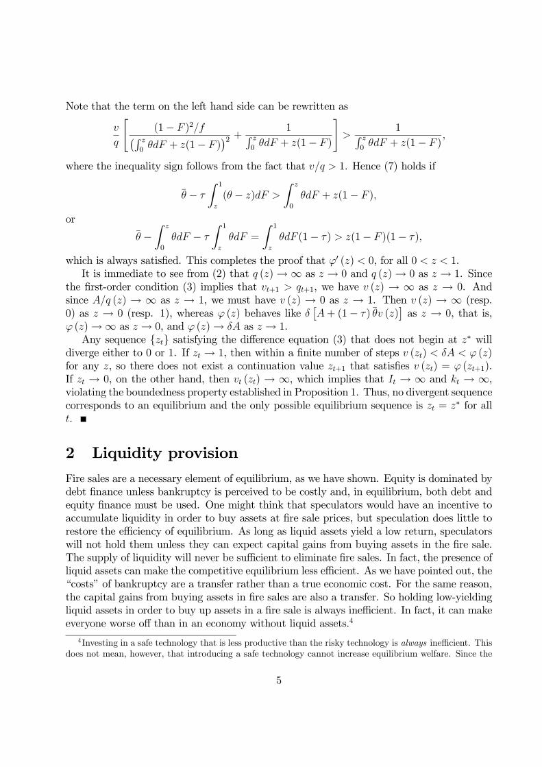
Note that the term on the left hand side can be rewritten as

"(1− )2¡R

0 + (1− )

¢2 + 1R 0 + (1− )

#

1R 0 + (1− )

where the inequality sign follows from the fact that 1. Hence (7) holds if

−

Z 1

( − )

Z

0

+ (1− )

or

−Z

0

−

Z 1

=

Z 1

(1− ) (1− )(1− )

which is always satisfied. This completes the proof that 0 () 0, for all 0 1.

It is immediate to see from (2) that ()→∞ as → 0 and ()→ 0 as → 1. Since

the first-order condition (3) implies that +1 +1, we have () → ∞ as → 0. And

since () → ∞ as → 1, we must have () → 0 as → 1. Then () → ∞ (resp.

0) as → 0 (resp. 1), whereas () behaves like £+ (1− ) ()

¤as → 0, that is,

()→∞ as → 0, and ()→ as → 1.

Any sequence {} satisfying the difference equation (3) that does not begin at ∗ willdiverge either to 0 or 1. If → 1, then within a finite number of steps () ()

for any , so there does not exist a continuation value +1 that satisfies () = (+1).

If → 0, on the other hand, then () → ∞, which implies that → ∞ and → ∞,violating the boundedness property established in Proposition 1. Thus, no divergent sequence

corresponds to an equilibrium and the only possible equilibrium sequence is = ∗ for all.

2 Liquidity provision

Fire sales are a necessary element of equilibrium, as we have shown. Equity is dominated by

debt finance unless bankruptcy is perceived to be costly and, in equilibrium, both debt and

equity finance must be used. One might think that speculators would have an incentive to

accumulate liquidity in order to buy assets at fire sale prices, but speculation does little to

restore the efficiency of equilibrium. As long as liquid assets yield a low return, speculators

will not hold them unless they can expect capital gains from buying assets in the fire sale.

The supply of liquidity will never be sufficient to eliminate fire sales. In fact, the presence of

liquid assets can make the competitive equilibrium less efficient. As we have pointed out, the

“costs” of bankruptcy are a transfer rather than a true economic cost. For the same reason,

the capital gains from buying assets in fire sales are also a transfer. So holding low-yielding

liquid assets in order to buy up assets in a fire sale is always inefficient. In fact, it can make

everyone worse off than in an economy without liquid assets.4

4Investing in a safe technology that is less productive than the risky technology is always inefficient. This

does not mean, however, that introducing a safe technology cannot increase equilibrium welfare. Since the

5

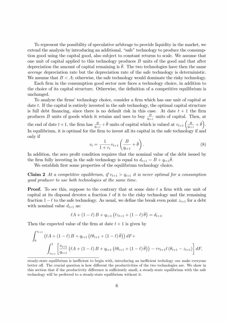
To represent the possibility of speculative arbitrage to provide liquidity in the market, we

extend the analysis by introducing an additional, “safe” technology to produce the consump-

tion good using the capital good, also subject to constant returns to scale. We assume that

one unit of capital applied to this technology produces units of the good and that after

depreciation the amount of capital remaining is . The two technologies have then the same

average depreciation rate but the depreciation rate of the safe technology is deterministic.

We assume that ; otherwise, the safe technology would dominate the risky technology.

Each firm in the consumption good sector now faces a technology choice, in addition to

the choice of its capital structure. Otherwise, the definition of a competitive equilibrium is

unchanged.

To analyze the firms’ technology choice, consider a firm which has one unit of capital at

date . If the capital is entirely invested in the safe technology, the optimal capital structure

is full debt financing, since there is no default risk in this case. At date + 1 the firm

produces units of goods which it retains and uses to buy +1

units of capital. Then, at

the end of date +1, the firm has +1

+ units of capital which is valued at +1

³

+1+ ´.

In equilibrium, it is optimal for the firm to invest all its capital in the safe technology if and

only if

=1

1 + +1

µ

+1+

¶ (8)

In addition, the zero profit condition requires that the nominal value of the debt issued by

the firm fully investing in the safe technology is equal to +1 = + +1

We establish first some properties of the equilibrium technology choice.

Claim 2 At a competitive equilibrium, if +1 +1 it is never optimal for a consumption

good producer to use both technologies at the same time.

Proof. To see this, suppose to the contrary that at some date a firm with one unit of

capital at its disposal devotes a fraction of it to the risky technology and the remaining

fraction 1− to the safe technology. As usual, we define the break even point +1 for a debtwith nominal value +1 as:

+ (1− ) + +1¡+1 + (1− )

¢= +1

Then the expected value of the firm at date + 1 is given byZ +1

0

¡+ (1− ) + +1

¡+1 + (1− )

¢¢+Z 1

+1

∙+1

+1

¡+ (1− ) + +1

¡+1 + (1− )

¢¢− +1 (+1 − +1)

¸

steady-state equilibrium is inefficient to begin with, introducing an inefficient techology can make everyone

better off. The crucial question is how different the productivities of the two technologies are. We show in

this section that if the productivity difference is sufficiently small, a steady-state equilibrium with the safe

technology will be preferred to a steady-state equilibrium without it.

6

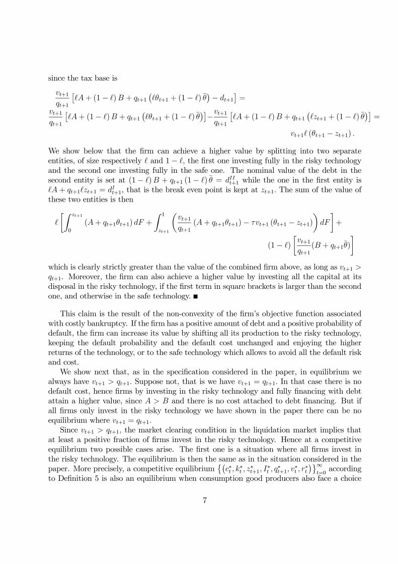
since the tax base is

+1

+1

£+ (1− ) + +1

¡+1 + (1− )

¢− +1¤=

+1

+1

£+ (1− ) + +1

¡+1 + (1− )

¢¤−+1+1

£+ (1− ) + +1

¡+1 + (1− )

¢¤=

+1 (+1 − +1)

We show below that the firm can achieve a higher value by splitting into two separate

entities, of size respectively and 1− the first one investing fully in the risky technology

and the second one investing fully in the safe one. The nominal value of the debt in the

second entity is set at (1− ) + +1 (1− ) = +1 while the one in the first entity is

+ +1+1 = +1, that is the break even point is kept at +1 The sum of the value of

these two entities is then

∙Z +1

0

(+ +1+1) +

Z 1

+1

µ+1

+1(+ +1+1)− +1 (+1 − +1)

¶

¸+

(1− )

∙+1

+1( + +1)

¸which is clearly strictly greater than the value of the combined firm above, as long as +1

+1. Moreover, the firm can also achieve a higher value by investing all the capital at its

disposal in the risky technology, if the first term in square brackets is larger than the second

one, and otherwise in the safe technology.

This claim is the result of the non-convexity of the firm’s objective function associated

with costly bankruptcy. If the firm has a positive amount of debt and a positive probability of

default, the firm can increase its value by shifting all its production to the risky technology,

keeping the default probability and the default cost unchanged and enjoying the higher

returns of the technology, or to the safe technology which allows to avoid all the default risk

and cost.

We show next that, as in the specification considered in the paper, in equilibrium we

always have +1 +1 Suppose not, that is we have +1 = +1 In that case there is no

default cost, hence firms by investing in the risky technology and fully financing with debt

attain a higher value, since and there is no cost attached to debt financing. But if

all firms only invest in the risky technology we have shown in the paper there can be no

equilibrium where +1 = +1

Since +1 +1 the market clearing condition in the liquidation market implies that

at least a positive fraction of firms invest in the risky technology. Hence at a competitive

equilibrium two possible cases arise. The first one is a situation where all firms invest in

the risky technology. The equilibrium is then the same as in the situation considered in the

paper. More precisely, a competitive equilibrium©¡∗

∗

∗+1

∗

∗+1

∗

∗

¢ª∞=0

according

to Definition 5 is also an equilibrium when consumption good producers also face a choice

7

between a risky and a safe technology provided the equilibrium values satisfy the following

condition, for all

∗ ≥1

1 + ∗∗+1

µ

∗+1+

¶ (9)

that is, no producer can gain at these prices by switching from the risky to the safe technology.

The second case arises when (9) is violated, in which case the competitive equilibrium is

different and entails a positive fraction (1−∗∗ ) ∈ (0 1) of firms using the safe technology. Inthis case, the equilibrium conditions need to be partly modified, in particular the liquidation

market clearing condition, which becomes

∗∗

Z ∗∗

0

= ∗∗ (1− (∗∗ )) + (1− ∗∗ ) (10)

to reflect the fact that the buyers of capital goods now include the solvent firms investing

in the risky technology and all the firms investing in the safe technology, as well as the

consumption good market clearing condition,

∗∗ ∗∗ + (1− ∗∗ )

∗∗ = ∗∗ + ∗∗ (11)

to reflect the differing productivities of the two technologies. In addition, condition (8),

requiring that firms must be indifferent between the safe and risky technologies, must also

hold.

We investigate in what follows the welfare properties of these equilibria. We show in

particular that the availability of an alternative, safe technology, which allows firms to avoid

the default risk, generates an additional source of inefficiency.

Claim 3 There exists a unique value of , denoted by 0, such that if ≤ we have

∗∗ = 1 in any steady-state equilibrium and the other values are (∗ ∗ ∗ ∗ ∗ ∗ ∗ ∗).By contrast, for some 0 and any ∈ ¡ +

¢, ∗∗ 1 and the consumption level ∗∗

is lower than the equilibrium level when the safe technology is not available, ∗.

Proof. When = the steady state equilibrium is the same as in the situation considered

in the paper, characterized in Proposition 7. Hence the equation determining the value of

the firm is still given by (as in Equilibrium condition 2):

∗ =

½Z ∗

0

(+ ∗) +Z 1

∗

µ∗

∗(+ ∗)− ∗ ( − ∗)

¶

¾(12)

The change in the equilibrium value of when is increased to + is obtained by

differentiating this equation with respect to and evaluating the derivative at = :

=

½µZ ∗

0

¶

+

µ1

∗

Z 1

∗(+ ∗)

¶

−µ∗

∗2

Z 1

∗∗

¶

−µ

Z 1

∗( − )

¶

¾

8

Rearranging, we getµ1−

∗

Z 1

∗∗(+ ∗) +

Z 1

∗( − )

¶

=

µZ ∗

0

− ∗

∗2

Z 1

∗

¶

Now, using the market-clearing condition

∗ =(1− (∗))R ∗0

() (13)

we see that

∗

Z 1

∗(+ ∗) =

∗

µ (1− (∗)) +

Z 1

∗∗

¶=

∗

µ∗Z ∗

0

+ ∗Z 1

∗

¶= 1

So,

1−

∗

Z 1

∗(+ ∗) +

Z 1

∗( − ) = 1− +

Z 1

∗( − )

1− 0

Similarly, again using (13),Z ∗

0

− ∗

∗2

Z 1

∗ =

Z

0

− ∗

∗ (1− (∗))

∗

Z ∗

0

−Z ∗

0

= 0

From these two inequalities, it follows that and

have opposite signs. Since

0

follows from

∗∗ =( + )

1−

we have proved that

0.

The change in the steady-state equilibrium consumption level is then obtained by differ-

entiating (11) with respect to and evaluating the derivative at = :

∗∗ = ∗∗ − ∗∗ + (−)∗∗∗ (14)

9

since ∗ = 1. The profit maximization condition ∗0 (∗) = 1 implies, as already shown in theprevious section, that a reduction in ∗∗ reduces ∗∗, and the law of motion ∗∗ = (∗∗)+∗∗

implies that a reduction in ∗∗ reduces ∗∗:

∗∗ =0 (∗)1−

∗∗

Also, ∗∗ ≤ 0 since ∗ = 1 at the equilibrium associated with = . Then inspection of

(14) yields

∗∗ ∗∗ − ∗∗

=

µ0 (∗)1−

− 1¶∗∗

=

Ã

∗¡1−

¢ − 1! ∗∗

so a sufficient condition for ∗∗ 0 is ∗¡1−

¢ . But it is clear from (12) that

∗ ≤ n1 + +

¡¢2+ · · · ¡¢ + · · ·o

=

1−

1−

This completes the proof of the proposition.

In what follows we focus again our attention on the case where (1) holds, that is consumers

are risk neutral. Hence, the critical value of , denoted by , is given by

=∗¡1−

¢

where ∗ is the price of liquidated capital at a steady-state equilibrium of the economy with nosafe technology. At this steady-state equilibrium price, (9) holds with equality when = ,

hence firms are indifferent between using the safe and risky technologies. At + , (9)

no longer holds, the steady-state equilibrium involves a positive fraction of firms 1− ∗∗ 0adopting the safe technology and a higher steady-state equilibrium value of ,

∗∗ =( + )

1− (15)

We showed in the proof of Claim 3 that equilibrium welfare is lower at a new steady-state

equilibrium than at the original one, with no safe technology. Since the original allocation,

with all firms investing in the risky technology, clearly remains feasible, this shows that the

equilibrium indeed exhibits an inefficient technology choice, with excessive investment in the

safe technology, as claimed.

10

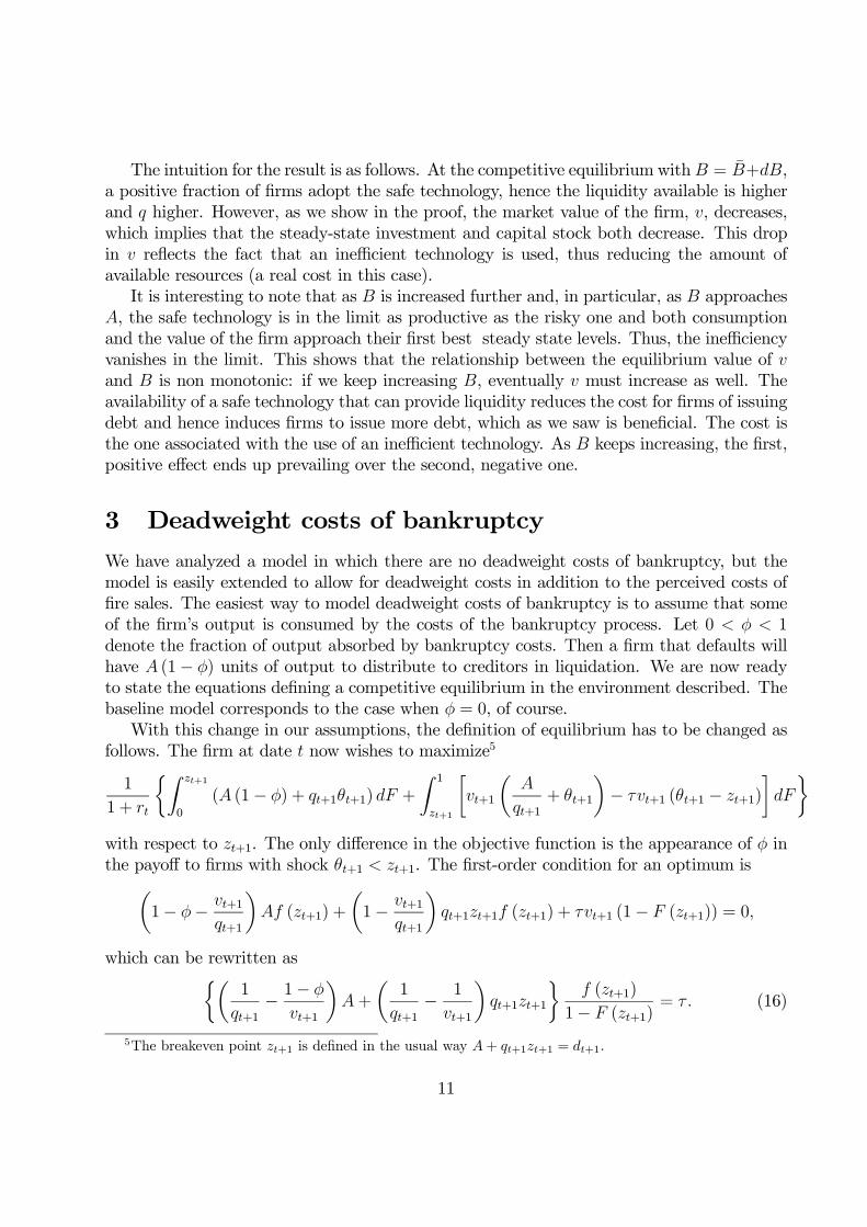
The intuition for the result is as follows. At the competitive equilibrium with = +,

a positive fraction of firms adopt the safe technology, hence the liquidity available is higher

and higher. However, as we show in the proof, the market value of the firm, , decreases,

which implies that the steady-state investment and capital stock both decrease. This drop

in reflects the fact that an inefficient technology is used, thus reducing the amount of

available resources (a real cost in this case).

It is interesting to note that as is increased further and, in particular, as approaches

, the safe technology is in the limit as productive as the risky one and both consumption

and the value of the firm approach their first best steady state levels. Thus, the inefficiency

vanishes in the limit. This shows that the relationship between the equilibrium value of

and is non monotonic: if we keep increasing , eventually must increase as well. The

availability of a safe technology that can provide liquidity reduces the cost for firms of issuing

debt and hence induces firms to issue more debt, which as we saw is beneficial. The cost is

the one associated with the use of an inefficient technology. As keeps increasing, the first,

positive effect ends up prevailing over the second, negative one.

3 Deadweight costs of bankruptcy

We have analyzed a model in which there are no deadweight costs of bankruptcy, but the

model is easily extended to allow for deadweight costs in addition to the perceived costs of

fire sales. The easiest way to model deadweight costs of bankruptcy is to assume that some

of the firm’s output is consumed by the costs of the bankruptcy process. Let 0 1

denote the fraction of output absorbed by bankruptcy costs. Then a firm that defaults will

have (1− ) units of output to distribute to creditors in liquidation. We are now ready

to state the equations defining a competitive equilibrium in the environment described. The

baseline model corresponds to the case when = 0, of course.

With this change in our assumptions, the definition of equilibrium has to be changed as

follows. The firm at date now wishes to maximize5

1

1 +

½Z +1

0

( (1− ) + +1+1) +

Z 1

+1

∙+1

µ

+1+ +1

¶− +1 (+1 − +1)

¸

¾with respect to +1. The only difference in the objective function is the appearance of in

the payoff to firms with shock +1 +1. The first-order condition for an optimum isµ1− − +1

+1

¶ (+1) +

µ1− +1

+1

¶+1+1 (+1) + +1 (1− (+1)) = 0

which can be rewritten as½µ1

+1− 1−

+1

¶+

µ1

+1− 1

+1

¶+1+1

¾ (+1)

1− (+1)= (16)

5The breakeven point +1 is defined in the usual way + +1+1 = +1.

11

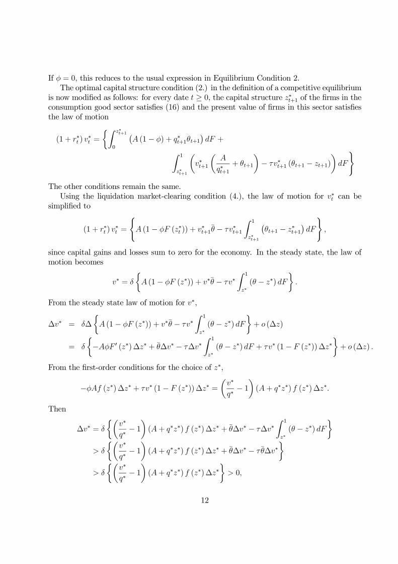
If = 0, this reduces to the usual expression in Equilibrium Condition 2.

The optimal capital structure condition (2.) in the definition of a competitive equilibrium

is now modified as follows: for every date ≥ 0, the capital structure ∗+1 of the firms in theconsumption good sector satisfies (16) and the present value of firms in this sector satisfies

the law of motion

(1 + ∗ ) ∗ =

½Z ∗+1

0

¡ (1− ) + ∗+1+1

¢ +Z 1

∗+1

µ∗+1

µ

∗+1+ +1

¶− ∗+1 (+1 − +1)

¶

)The other conditions remain the same.

Using the liquidation market-clearing condition (4.), the law of motion for ∗ can besimplified to

(1 + ∗ ) ∗ =

( (1− (∗ )) + ∗+1 − ∗+1

Z 1

∗+1

¡+1 − ∗+1

¢

)

since capital gains and losses sum to zero for the economy. In the steady state, the law of

motion becomes

∗ =

½ (1− (∗)) + ∗ − ∗

Z 1

∗( − ∗)

¾

From the steady state law of motion for ∗,

∆∗ = ∆

½ (1− (∗)) + ∗ − ∗

Z 1

∗( − ∗)

¾+ (∆)

=

½− 0 (∗)∆∗ + ∆∗ − ∆∗

Z 1

∗( − ∗) + ∗ (1− (∗))∆∗

¾+ (∆)

From the first-order conditions for the choice of ∗,

− (∗)∆∗ + ∗ (1− (∗))∆∗ =

µ∗

∗− 1¶(+ ∗∗) (∗)∆∗

Then

∆∗ =

½µ∗

∗− 1¶(+ ∗∗) (∗)∆∗ + ∆∗ − ∆∗

Z 1

∗( − ∗)

¾

½µ∗

∗− 1¶(+ ∗∗) (∗)∆∗ + ∆∗ − ∆∗

¾

½µ∗

∗− 1¶(+ ∗∗) (∗)∆∗

¾ 0

12

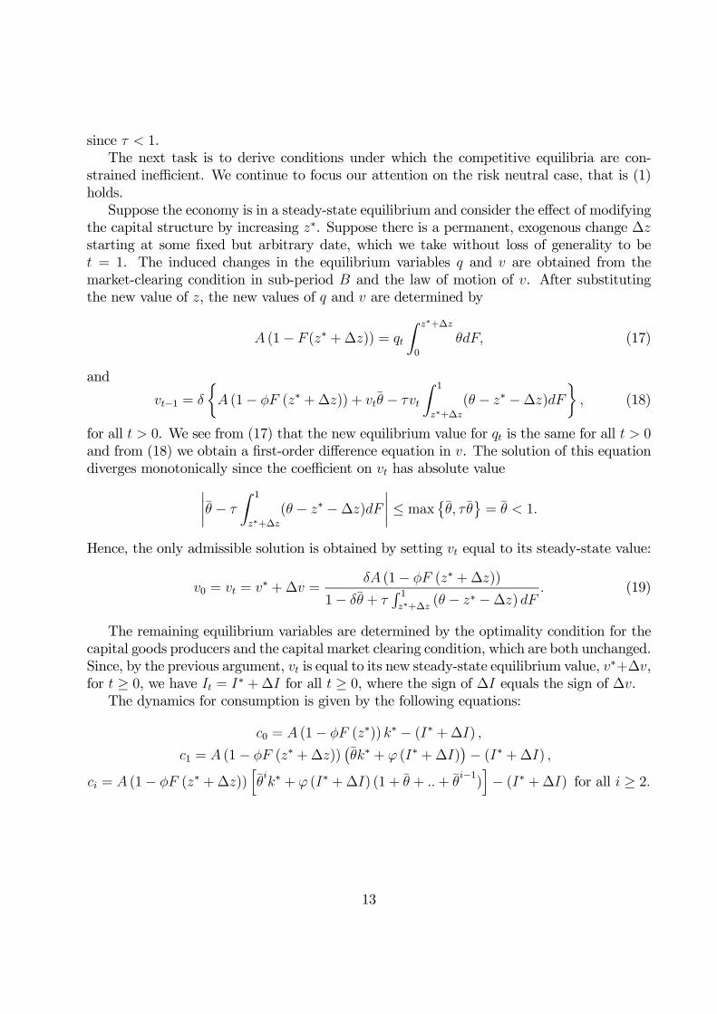
since 1.

The next task is to derive conditions under which the competitive equilibria are con-

strained inefficient. We continue to focus our attention on the risk neutral case, that is (1)

holds.

Suppose the economy is in a steady-state equilibrium and consider the effect of modifying

the capital structure by increasing ∗. Suppose there is a permanent, exogenous change ∆

starting at some fixed but arbitrary date, which we take without loss of generality to be

= 1. The induced changes in the equilibrium variables and are obtained from the

market-clearing condition in sub-period and the law of motion of . After substituting

the new value of , the new values of and are determined by

(1− (∗ +∆)) =

Z ∗+∆

0

(17)

and

−1 =

½ (1− (∗ +∆)) + −

Z 1

∗+∆

( − ∗ −∆)

¾ (18)

for all 0. We see from (17) that the new equilibrium value for is the same for all 0

and from (18) we obtain a first-order difference equation in . The solution of this equation

diverges monotonically since the coefficient on has absolute value¯ −

Z 1

∗+∆

( − ∗ −∆)

¯≤ max© ª = 1

Hence, the only admissible solution is obtained by setting equal to its steady-state value:

0 = = ∗ +∆ = (1− (∗ +∆))

1− + R 1∗+∆

( − ∗ −∆) (19)

The remaining equilibrium variables are determined by the optimality condition for the

capital goods producers and the capital market clearing condition, which are both unchanged.

Since, by the previous argument, is equal to its new steady-state equilibrium value, ∗+∆,

for ≥ 0, we have = ∗ +∆ for all ≥ 0, where the sign of ∆ equals the sign of ∆.

The dynamics for consumption is given by the following equations:

0 = (1− (∗)) ∗ − (∗ +∆)

1 = (1− (∗ +∆))¡∗ + (∗ +∆)

¢− (∗ +∆)

= (1− (∗ +∆))h∗ + (∗ +∆) (1 + + +

−1)i− (∗ +∆) for all ≥ 2

13

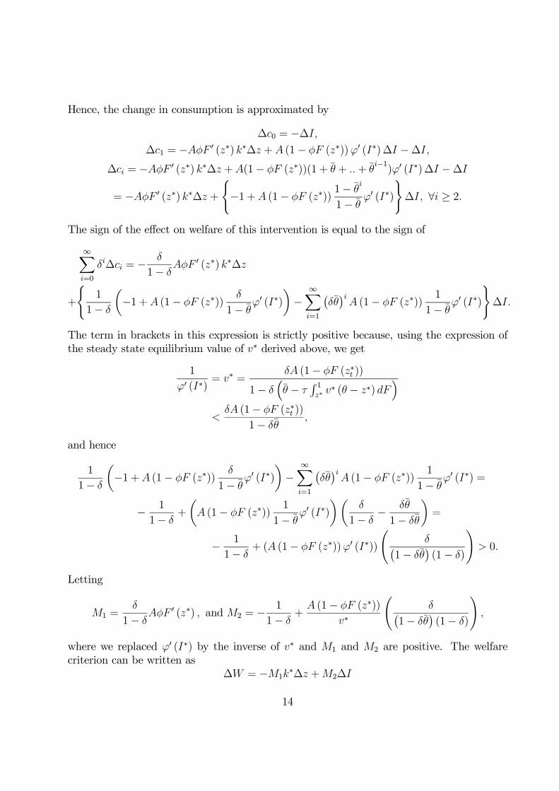
Hence, the change in consumption is approximated by

∆0 = −∆

∆1 = − 0 (∗) ∗∆ + (1− (∗))0 (∗)∆ −∆

∆ = − 0 (∗) ∗∆ +(1− (∗))(1 + + + −1)0 (∗)∆ −∆

= − 0 (∗) ∗∆ +

(−1 + (1− (∗))

1−

1− 0 (∗)

)∆ ∀ ≥ 2

The sign of the effect on welfare of this intervention is equal to the sign of

∞X=0

∆ = −

1− 0 (∗) ∗∆

+

(1

1−

µ−1 + (1− (∗))

1− 0 (∗)

¶−

∞X=1

¡¢ (1− (∗))

1

1− 0 (∗)

)∆

The term in brackets in this expression is strictly positive because, using the expression of

the steady state equilibrium value of ∗ derived above, we get

1

0 (∗)= ∗ =

(1− (∗ ))

1− ³ −

R 1∗

∗ ( − ∗) ´

(1− (∗ ))

1−

and hence

1

1−

µ−1 + (1− (∗))

1− 0 (∗)

¶−

∞X=1

¡¢ (1− (∗))

1

1− 0 (∗) =

− 1

1− +

µ (1− (∗))

1

1− 0 (∗)

¶µ

1− −

1−

¶=

− 1

1− + ( (1− (∗))0 (∗))

á

1− ¢(1− )

! 0

Letting

1 =

1− 0 (∗) and 2 = − 1

1− +

(1− (∗))∗

á

1− ¢(1− )

!

where we replaced 0 (∗) by the inverse of ∗ and 1 and 2 are positive. The welfare

criterion can be written as

∆ = −1∗∆ +2∆

14

so ∆ 0 if and only if∆

∆

1

∗

1

2

In other words, an increase in ∗ will increase welfare if and only if the response of investmentto the change in capital structure is sufficiently large.

To illustrate, suppose the production function for capital goods is given by

() =1

1− 1−

Then ∗ = (∗) and ∗ = (∗)1 . The equilibrium variables ∗, ∗ and ∗ are defined by the

market-clearing condition

∗ = (1− ())R ∗

0

the steady-state law of motion

∗ = (1− (∗))

1− ³ −

R 1∗ ( − ∗)

´ and the first-order condition½µ

1

∗− 1−

∗

¶+

µ1

∗− 1

∗

¶∗∗

¾ (∗)

1− (∗)=

Note that this subsystem does not depend on the parameter . Then the constants 1 and

2 are also independent of (when we have substituted 1∗ for 0 (∗)).

We can approximate ∆∆ can be approximated by

, and since

0 is indepen-

dent of , the necessary and sufficient condition for an increase in welfare is

1

∗

1

2

∗

∗

where the right hand side is independent of . Now

∗ = (∗)1−

=

³(∗)

1

´1−(1− )

¡1−

¢and

=1

(∗)

1−

15

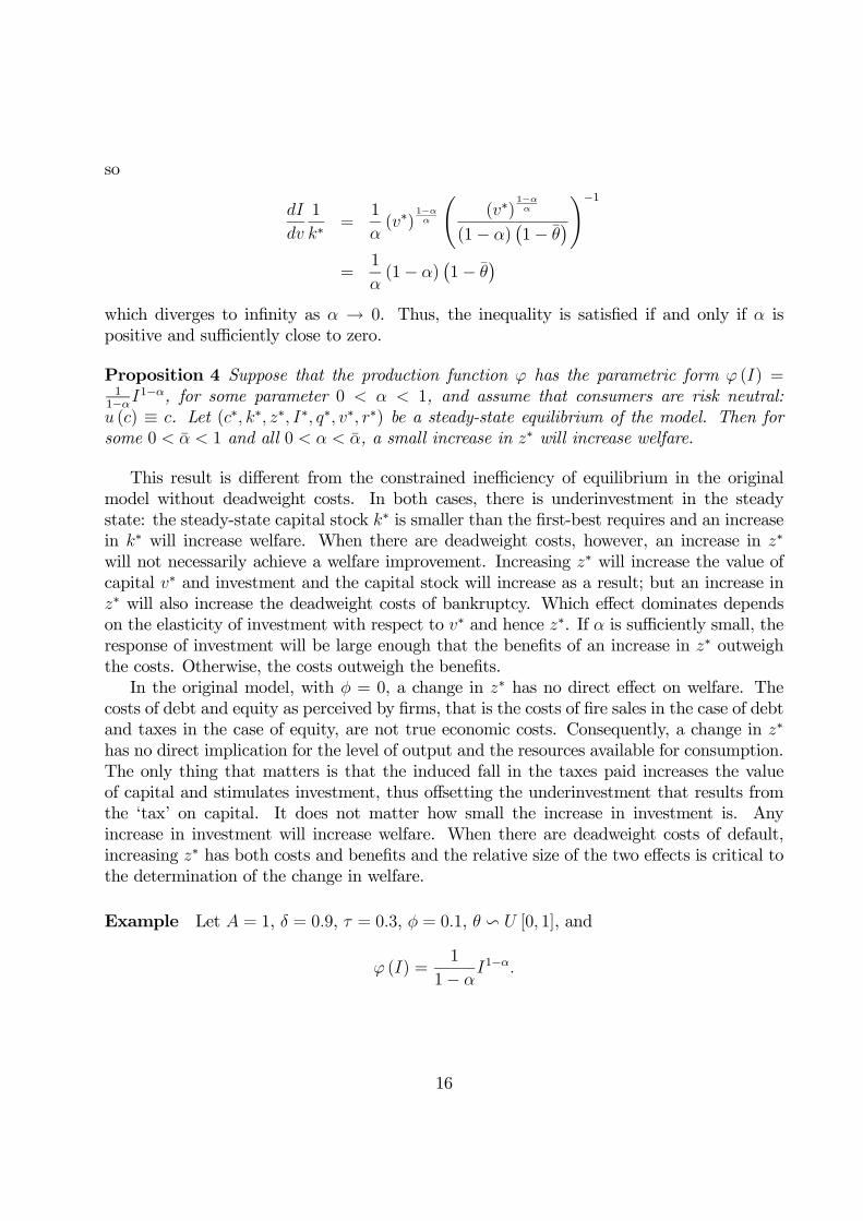
so

1

∗=

1

(∗)

1−

Ã(∗)

1−

(1− )¡1−

¢!−1=

1

(1− )

¡1−

¢which diverges to infinity as → 0. Thus, the inequality is satisfied if and only if is

positive and sufficiently close to zero.

Proposition 4 Suppose that the production function has the parametric form () =11−

1−, for some parameter 0 1, and assume that consumers are risk neutral:

() ≡ . Let (∗ ∗ ∗ ∗ ∗ ∗ ∗) be a steady-state equilibrium of the model. Then for

some 0 1 and all 0 , a small increase in ∗ will increase welfare.

This result is different from the constrained inefficiency of equilibrium in the original

model without deadweight costs. In both cases, there is underinvestment in the steady

state: the steady-state capital stock ∗ is smaller than the first-best requires and an increasein ∗ will increase welfare. When there are deadweight costs, however, an increase in ∗

will not necessarily achieve a welfare improvement. Increasing ∗ will increase the value ofcapital ∗ and investment and the capital stock will increase as a result; but an increase in∗ will also increase the deadweight costs of bankruptcy. Which effect dominates dependson the elasticity of investment with respect to ∗ and hence ∗. If is sufficiently small, theresponse of investment will be large enough that the benefits of an increase in ∗ outweighthe costs. Otherwise, the costs outweigh the benefits.

In the original model, with = 0, a change in ∗ has no direct effect on welfare. Thecosts of debt and equity as perceived by firms, that is the costs of fire sales in the case of debt

and taxes in the case of equity, are not true economic costs. Consequently, a change in ∗

has no direct implication for the level of output and the resources available for consumption.

The only thing that matters is that the induced fall in the taxes paid increases the value

of capital and stimulates investment, thus offsetting the underinvestment that results from

the ‘tax’ on capital. It does not matter how small the increase in investment is. Any

increase in investment will increase welfare. When there are deadweight costs of default,

increasing ∗ has both costs and benefits and the relative size of the two effects is critical tothe determination of the change in welfare.

Example Let = 1, = 09, = 03, = 01, v [0 1], and

() =1

1− 1−

16

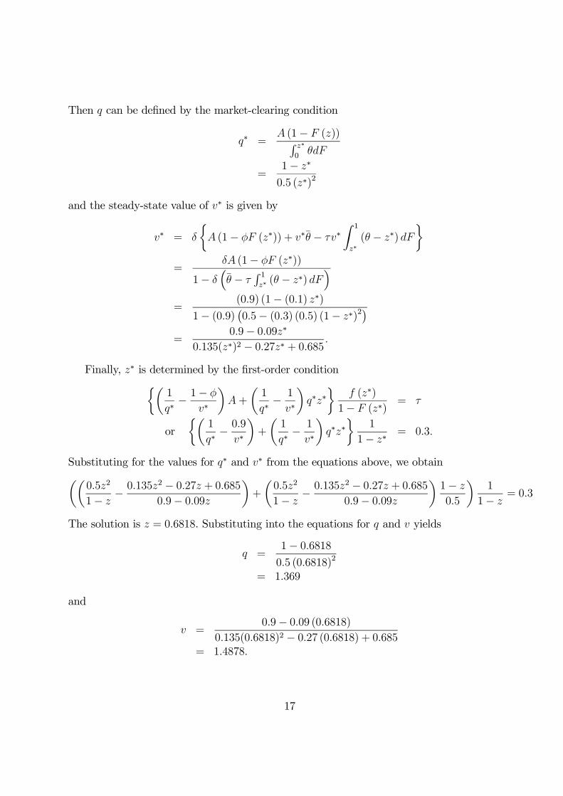
Then can be defined by the market-clearing condition

∗ = (1− ())R ∗

0

=1− ∗

05 (∗)2

and the steady-state value of ∗ is given by

∗ =

½ (1− (∗)) + ∗ − ∗

Z 1

∗( − ∗)

¾=

(1− (∗))

1− ³ −

R 1∗ ( − ∗)

´=

(09) (1− (01) ∗)1− (09) ¡05− (03) (05) (1− ∗)2

¢=

09− 009∗0135(∗)2 − 027∗ + 0685

Finally, ∗ is determined by the first-order condition½µ1

∗− 1−

∗

¶+

µ1

∗− 1

∗

¶∗∗

¾ (∗)

1− (∗)=

or

½µ1

∗− 09

∗

¶+

µ1

∗− 1

∗

¶∗∗

¾1

1− ∗= 03

Substituting for the values for ∗ and ∗ from the equations above, we obtainµµ052

1− − 0135

2 − 027 + 068509− 009

¶+

µ052

1− − 0135

2 − 027 + 068509− 009

¶1−

05

¶1

1− = 03

The solution is = 06818. Substituting into the equations for and yields

=1− 0681805 (06818)

2

= 1369

and

=09− 009 (06818)

0135(06818)2 − 027 (06818) + 0685= 14878

17

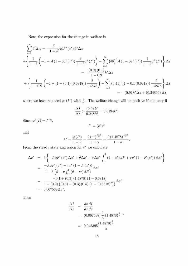
Now, the expression for the change in welfare is

∞X=0

∆ = −

1− 0 (∗) ∗∆

+

(1

1−

µ−1 + (1− (∗))

1− 0 (∗)

¶−

∞X=1

¡¢ (1− (∗))

1

1− 0 (∗)

)∆

= −(09) (01)1− 09 ∗∆

+

(1

1− 09µ−1 + (1− (01) (06818)) 2

14878

¶−

∞X=1

(045)(1− 01 (06818)) 2

14878

)∆

= − (09) ∗∆ + (024866)∆

where we have replaced 0 (∗) with 1∗ . The welfare change will be positive if and only if

∆

∆(09) ∗

024866= 36194∗

Since 0 () = −,

∗ = (∗)1

and

∗ = (∗)1−

=2 (∗)

1−

1− =2 (14878)

1−

1−

From the steady state expression for ∗ we calculate

∆∗ =

½− 0 (∗)∆∗ + ∆∗ − ∆∗

Z 1

∗( − ∗) + ∗ (1− (∗))∆∗

¾=− 0 (∗) + ∗ (1− (∗))

1− ³ −

R 1∗ ( − ∗)

´ ∆∗

=−01 + (03) (14878) (1− 06818)

1− (09) ¡(05)− (03) (05) ¡1− (06818)2¢¢∆∗

= 0067538∆∗

Then

∆

∆=

= (0067538)1

(14878)

1−1

= 0045395(14878)

1

18

Then the condition for a welfare improvement becomes

(0045395)(14878)

1

36194∗

= (048476)2 (14878)

1−

1−

which is satisfied if and only if 0 0065125.

4 Aggregate uncertainty

To introduce aggregate uncertainty, we assume that the distribution of depreciation rates is

subject to aggregate shocks. Let {} be a series of i.i.d. random variables taking values in

a finite set S with probability density π = {}∈S . After production of the consumptiongood by an arbitrary firm at date , one unit of capital is reduced to units of capital,

where is the usual idiosyncractic shock and is a common shock. We assume that and are independent for each and .

In this environment both the stock of capital, consumption, investment and prices will

depend on the aggregate shock. We show in what follows that, again under the assumption

that consumers are risk neutral, that is (1) holds, an equilibrium exists where prices are

inversely related to the realization of the aggregate state, +1 () = +1, +1 () = +1

for any ∈ S and some +1 +1 while the default threshold is independent of the state,+1 () = +1, for any .

The market-clearing condition in the liquidation market in sub-period (Equilibrium

Condition 4) in every state is then

+1 () = (1− (+1))R +10

+1

or, using the above specification,

+1 = (1− (+1))R +1

0+1

The tax base is again the value of the firm’s equity at the beginning of sub-period ,

whenever it is non negative, that is, the difference between the value of capital owned by the

firm and the value of (renegotiated) debt

+1 ()

µ

+1 ()+ +1

¶− +1 ()

µ+1

+1()

¶

Hence, the corporate income tax payment due at date + 1 in state , using the definition

19

of the default threshold, + +1 () +1 = +1 is

max

½+1 ()

µ

+1 ()+ +1

¶− +1 ()

µ+1

+1 ()

¶ 0

¾= max

½+1 ()

+1 ()(+ +1 () +1 −− +1 () +1) 0

¾= max {+1 (+1 − +1) 0}

The optimal capital structure is then obtained as a solution of the following problem of

maximizing the the firm’s market value at

max+1

X∈S

()

( R +10

(+ +1 () +1) +R 1+1

h+1 ()

³

+1()+ +1

´− +1 () (+1 − +1)

i ) =

Z +1

0

(+ +1+1) +

Z 1

+1

∙+1

µ

+1+ +1

¶− +1 (+1 − +1)

¸

whose first-order condition is

½µ1− +1

+1

¶(+ +1+1) (+1) + +1+1 (1− (+1))

¾= 0

The above argument shows that the equations determining the firms’ capital structure,

the law of motion of and the price of liquidated capital are the same as in Definition

5 of a competitive equilibrium, with no aggregate uncertainty and do not depend on

In contrast, we see from the new expressions of Equilibrium Conditions 1 (the (interior)

condition for the firms’ optimum in the capital goods sector),

0 (()) = 1 (20)

and 6. (capital market clearing)

+1(+1) = (

) + 0 (())

that depends on and does too (as well as on the history of realizations of ), and so .

The same argument as the one in the paper for the case of no aggregate risk then implies

that increases in response to a (marginal) increases of above its equilibrium value. Hence

from (20) we see that () also increases, for every . An extension of the argument in the

main text then allows to show that agents’ welfare also increases, as a result.

5 The corporate income tax

The presence of fire sales and stochastic depreciation makes it difficult to incorporate a

realistic version of the corporate income tax in our baseline model. In the main text we

20

chose then to use a tax on the value of equity as a proxy for the corporate income tax.

In this section, we investigate in more detail the relationship between taxes on corporate

earnings (after interest and depreciation) and taxes on the value of equity. To keep things

simple, we focus on the steady state and assume that the depreciation rate is non-stochastic,

given by a constant 1− Hence there are no fire sales, = .

Suppose a firm has one unit of capital at the end of date 0. One unit of capital produces

units of the good. The depreciation in period 1 is (1− ) . In the steady state, the

interest rate satisfies 1 (1 + ) = or = (1− ) . If is the face value of the debt

issued, the amount borrowed is and the interest on the debt is

=1−

= (1− )

Since capital is constant (depreciation is replaced by new investment), the firm’s earnings

are constant over time and equal to

= − (1− ) − (1− )

at each date . With a proportional tax on corporate earnings, the tax paid at date is

and the present value of future taxes, at the end of date 1, is

∞X=1

=

∞X=1

(− (1− ) − (1− ) )

=

1− (− (1− )− (1− ))

Let denote the value of equity at the end of a period (i.e., in sub-period ). This

clearly satisfies

= (1− )

1− (− (1− )− (1− ))

If instead a tax is imposed on the value of equity at the rate 0 each period, the tax billin period is 0 , where

denotes the value of equity in this case, and earnings after tax

are

= − (1− ) − (1− ) − 0

Then satisfies

=

∞X=1

(− (1− ) − (1− ) − 0)

=

1− (− (1− ) − (1− ) − 0)

and so

=

1− + 0(− (1− ) − (1− ) )

21

Then it is clear that = if and only if

1−

1− =

1

1− + 0

or

= 0

1− + 0

When this condition is satisfied, it seems intuitively clear and can be shown by direct calcu-

lations that the present value of taxes is the same under each tax regime.

6 Long-term debt and debt covenants

In the main text we considered the case where all debt takes the form of bonds with a

maturity of one period. Thus, all debt is due for repayment one period after it is issued. If

instead debt took the form of bonds with a maturity of 1 periods, then in a steady state,

one -th of the debt would be due for repayment each period. The face value of debt issued

in equilibrium might be greater if the maturity were periods rather than one, but, other

things being equal, increasing the maturity of the debt tends to reduce the amount that had

to be repaid in any one period. Thus, one might expect that, other things being equal, the

probability of default and the severity of fire sales would be less if firms issued bonds with

longer maturities.

In this case however, the ceteris paribus assumption is not particularly plausible. If

the severity of fire sales decreases, firms will have an incentive to increase the face value

of debt they issue. But there is a more serious problem with long term debt. It creates a

moral hazard for creditors. Creditors have little control over the firm as long as the debt

contract only requires it to pay the agreed interest and principal. This allows equity holders

to enrich themselves at the expense of creditors. Consider the extreme case of perpetual

bonds that pay interest at the rate = 1− on principal of per unit of capital. As long as

the firm pays the required interest each period, there is nothing to stop the equity holders

from paying themselves large dividends by selling off capital until the firm is worthless. It is

because of this possibility that long-term bond contracts typically contain multiple covenants

controlling the behavior of the firm. For example, covenants might restrict the firm’s ability

to issue new debt and to alter the seniority of the existing debt. They might also require the

firm to maintain an adequate ratio of earnings to interest payments, the so-called interest

coverage ratio, and to maintain the value of the firm’s assets in relation to the value of debt.

If any of these covenants is violated, the firm is technically in default and the repayment of

the debt is accelerated, i.e., repayment of the entire debt is due immediately. Such technical

defaults rarely result in the bankruptcy of the firm (Roberts and Sufi, 2009). Rather, they

force a renegotiation in which the firm may be forced to pay a higher interest rate, put up

more collateral, or make some other change in its behavior or commitments.

One plausible covenant in our model would require the firm not only to make regular

interest payments but also to maintain the level of the firm’s assets. This will prevent the

22

firm from selling off assets and paying the proceeds to equity holders. In the case of a firm

with one unit of capital and a depreciation rate 1 − , the firm will have to pay 1 − in

interest and invest (1− ) to replace the depreciated capital stock. Since the firm’s gross

revenue is , the firm will only be able to satisfy the covenants if −(1− ) −(1− ) ≥ 0.Note that the covenant is specified assuming that the firm can buy ‘used’ capital goods at

the lower price of . If the inequality is not satisfied, the firm is technically in default and

will be forced to renegotiate with the creditors. Let ∗∗ denote the value of at which thefirm is just able to satisfy the covenants. That is,

− (1− ∗∗) − (1− ) = 0

We assume that, if the firm is forced to renegotiate, it makes a take-it-or-leave-it offer that

is accepted or rejected by the creditors subject to the rules that we laid down in the model

considered in the main text. There we found that renegotiation succeeds if and only if ≥ ∗,where

− ∗ =

If ∗∗ ∗, then renegotiation occurs and fails if and only if ∗, just as in the modelwith one-period debt. In that case, even though the debt consists of perpetual bonds, the

principal of which is never repaid, default occurs precisely as it does with one-period debt.

In this case, there would exist an equilibrium that is essentially the same as the equilibrium

in the baseline model. On the other hand, if ∗ ∗∗, then renegotiation does not occur forsome values of where it would fail. In other words, the probability of default will be strictly

lower than it would be in the model with one-period debt, other things being equal. Other

things may not be equal, however. In the first place, the firm has an incentive to increase

the face of debt issued, because it does not have to renegotiate in the states ∗ ∗∗,where default would occur with one-period bonds. An increase in the face value of debt will

lead to changes in equilibrium prices, however, and that will lead to further changes in the

capital structure. The final effect of the switch to longer maturity debt is not clear.

Whichever case, ∗ ∗∗ or ∗ ∗∗, occurs in equilibrium, it is clear that =

min {∗ ∗∗} plays the role of the breakeven level in the model with one-period debt. Evenin the extreme case of perpetual bonds, with no requirement to repay principal, the qual-

itative behavior of the model will be similar to the model considered in the main text

with one-period debt. Firms will be forced to renegotiate and will be forced to liquidate if

= min {∗ ∗∗}. Long-term debt with this bond covenant functions essentially like

short-term debt as far as default is concerned.

References

[1] Roberts, Michael R. and Amir Sufi (2009) “Renegotiation of financial contracts: Evidence

from private credit agreements” Journal of Financial Economics 93(2), 159—184

23

will not necessarily achieve a welfare improvement. Increasing ∗ will increase the value of

capital ∗ and investment and the capital stock will increase as a result; but an increase in

∗ will also increase the deadweight costs of bankruptcy. Which effect dominates depends

on the elasticity of investment with respect to ∗ and hence ∗. If is sufficiently small, the

response of investment will be large enough that the benefits of an increase in ∗ outweigh

the costs. Otherwise, the costs outweigh the benefits.

In the original model, with = 0, a change in ∗ has no direct effect on welfare. The

costs of debt and equity as perceived by firms, that is the costs of fire sales in the case of debt

and taxes in the case of equity, are not true economic costs. Consequently, a change in ∗

has no direct implication for the level of output and the resources available for consumption.

The only thing that matters is that the induced fall in the taxes paid increases the value

of capital and stimulates investment, thus offsetting the underinvestment that results from

the ‘tax’ on capital. It does not matter how small the increase in investment is. Any

increase in investment will increase welfare. When there are deadweight costs of default,

increasing ∗ has both costs and benefits and the relative size of the two effects is critical to

the determination of the change in welfare.

Example Let = 1, = 09, = 03, = 01, v [0 1], and

() =1

1− 1−

24

Then can be defined by the market-clearing condition

∗ = (1− ())R ∗

0

=1− ∗

05 (∗)2

and the steady-state value of ∗ is given by

∗ =

½ (1− (∗)) + ∗ − ∗

Z 1

∗( − ∗)

¾=

(1− (∗))

1− ³ −

R 1∗ ( − ∗)

´=

(09) (1− (01) ∗)1− (09) ¡05− (03) (05) (1− ∗)2

¢=

09− 009∗0135(∗)2 − 027∗ + 0685

Finally, ∗ is determined by the first-order condition

½µ1

∗− 1−

∗

¶+

µ1

∗− 1

∗

¶∗∗

¾ (∗)

1− (∗)=

or

½µ1

∗− 09

∗

¶+

µ1

∗− 1

∗

¶∗∗

¾1

1− ∗= 03

Substituting for the values for ∗ and ∗ from the equations above, we obtain

µµ052

1− − 0135

2 − 027 + 068509− 009

¶+

µ052

1− − 0135

2 − 027 + 068509− 009

¶1−

05

¶1

1− = 03

The solution is = 06818. Substituting into the equations for and yields

=1− 0681805 (06818)

2

= 1369

25

and

=09− 009 (06818)

0135(06818)2 − 027 (06818) + 0685= 14878

Now, the expression for the change in welfare is

∞X=0

∆ = −

1− 0 (∗) ∗∆

+

(1

1−

µ−1 + (1− (∗))

1− 0 (∗)

¶−

∞X=1

¡¢ (1− (∗))

1

1− 0 (∗)

)∆

= −(09) (01)1− 09 ∗∆

+

(1

1− 09µ−1 + (1− (01) (06818)) 2

14878

¶−

∞X=1

(045)(1− 01 (06818)) 2

14878

)∆

= − (09) ∗∆ + (024866)∆

where we have replaced 0 (∗) with 1∗ . The welfare change will be positive if and only if

∆

∆(09) ∗

024866= 36194∗

Since 0 () = −,

∗ = (∗)1

and

∗ = (∗)1−

=2 (∗)

1−

1− =2 (14878)

1−

1−

26

From the steady state expression for ∗ we calculate

∆∗ =

½− 0 (∗)∆∗ + ∆∗ − ∆∗

Z 1

∗( − ∗) + ∗ (1− (∗))∆∗

¾=− 0 (∗) + ∗ (1− (∗))

1− ³ −

R 1∗ ( − ∗)

´ ∆∗

=−01 + (03) (14878) (1− 06818)

1− (09) ¡(05)− (03) (05) ¡1− (06818)2¢¢∆∗

= 0067538∆∗

Then

∆

∆=

= (0067538)1

(14878)

1−1

= 0045395(14878)

1

Then the condition for a welfare improvement becomes

(0045395)(14878)

1

36194∗

= (048476)2 (14878)

1−

1−

which is satisfied if and only if 0 0065125.

4 Aggregate uncertainty

To introduce aggregate uncertainty, we assume that the distribution of depreciation rates is

subject to aggregate shocks. Let {} be a series of i.i.d. random variables taking values in

a finite set S with probability density π = {}∈S . After production of the consumption

27

good by an arbitrary firm at date , one unit of capital is reduced to units of capital,

where is the usual idiosyncractic shock and is a common shock. We assume that

and are independent for each and .

In this environment both the stock of capital, consumption, investment and prices will

depend on the aggregate shock. We show in what follows that, again under the assumption

that consumers are risk neutral, that is (1) holds, an equilibrium exists where prices are

inversely related to the realization of the aggregate state, +1 () = +1, +1 () = +1

for any ∈ S and some +1 +1 while the default threshold is independent of the state,

+1 () = +1, for any .

The market-clearing condition in the liquidation market in sub-period (Equilibrium

Condition 4) in every state is then

+1 () = (1− (+1))R +10

+1

or, using the above specification,

+1 = (1− (+1))R +1

0+1

The tax base is again the value of the firm’s equity at the beginning of sub-period ,

whenever it is non negative, that is, the difference between the value of capital owned by the

firm and the value of (renegotiated) debt

+1 ()

µ

+1 ()+ +1

¶− +1 ()

µ+1

+1()

¶

Hence, the corporate income tax payment due at date + 1 in state , using the definition

28

of the default threshold, + +1 () +1 = +1 is

max

½+1 ()

µ

+1 ()+ +1

¶− +1 ()

µ+1

+1 ()

¶ 0

¾= max

½+1 ()

+1 ()(+ +1 () +1 −− +1 () +1) 0

¾= max {+1 (+1 − +1) 0}

The optimal capital structure is then obtained as a solution of the following problem of

maximizing the the firm’s market value at

max+1

X∈S

()

⎧⎪⎪⎨⎪⎪⎩R +10

(+ +1 () +1) +R 1+1

h+1 ()

³

+1()+ +1

´− +1 () (+1 − +1)

i⎫⎪⎪⎬⎪⎪⎭ =

Z +1

0

(+ +1+1) +

Z 1

+1

∙+1

µ

+1+ +1

¶− +1 (+1 − +1)

¸

whose first-order condition is

½µ1− +1

+1

¶(+ +1+1) (+1) + +1+1 (1− (+1))

¾= 0

The above argument shows that the equations determining the firms’ capital structure,

the law of motion of and the price of liquidated capital are the same as in Definition

5 of a competitive equilibrium, with no aggregate uncertainty and do not depend on

In contrast, we see from the new expressions of Equilibrium Conditions 1 (the (interior)

condition for the firms’ optimum in the capital goods sector),

0 (()) = 1 (20)

and 6. (capital market clearing)

+1(+1) = (

) + 0 (())

29

that depends on and does too (as well as on the history of realizations of ), and so .

The same argument as the one in the paper for the case of no aggregate risk then implies

that increases in response to a (marginal) increases of above its equilibrium value. Hence

from (20) we see that () also increases, for every . An extension of the argument in the

main text then allows to show that agents’ welfare also increases, as a result.

5 The corporate income tax

The presence of fire sales and stochastic depreciation makes it difficult to incorporate a

realistic version of the corporate income tax in our baseline model. In the main text we

chose then to use a tax on the value of equity as a proxy for the corporate income tax.

In this section, we investigate in more detail the relationship between taxes on corporate

earnings (after interest and depreciation) and taxes on the value of equity. To keep things

simple, we focus on the steady state and assume that the depreciation rate is non-stochastic,

given by a constant 1− Hence there are no fire sales, = .

Suppose a firm has one unit of capital at the end of date 0. One unit of capital produces

units of the good. The depreciation in period 1 is (1− ) . In the steady state, the

interest rate satisfies 1 (1 + ) = or = (1− ) . If is the face value of the debt

issued, the amount borrowed is and the interest on the debt is

=1−

= (1− )

Since capital is constant (depreciation is replaced by new investment), the firm’s earnings

30

are constant over time and equal to

= − (1− ) − (1− )

at each date . With a proportional tax on corporate earnings, the tax paid at date is

and the present value of future taxes, at the end of date 1, is

∞X=1

=

∞X=1

(− (1− ) − (1− ) )

=

1− (− (1− )− (1− ))

Let denote the value of equity at the end of a period (i.e., in sub-period ). This

clearly satisfies

= (1− )

1− (− (1− )− (1− ))

If instead a tax is imposed on the value of equity at the rate 0 each period, the tax bill

in period is 0 , where denotes the value of equity in this case, and earnings after tax

are

= − (1− ) − (1− ) − 0

Then satisfies

=

∞X=1

(− (1− ) − (1− ) − 0)

=

1− (− (1− ) − (1− ) − 0)

and so

=

1− + 0(− (1− ) − (1− ) )

31

Then it is clear that = if and only if

1−

1− =

1

1− + 0

or

= 0

1− + 0

When this condition is satisfied, it seems intuitively clear and can be shown by direct calcu-

lations that the present value of taxes is the same under each tax regime.

6 Long-term debt and debt covenants

In the main text we considered the case where all debt takes the form of bonds with a

maturity of one period. Thus, all debt is due for repayment one period after it is issued. If

instead debt took the form of bonds with a maturity of 1 periods, then in a steady state,

one -th of the debt would be due for repayment each period. The face value of debt issued

in equilibrium might be greater if the maturity were periods rather than one, but, other

things being equal, increasing the maturity of the debt tends to reduce the amount that had

to be repaid in any one period. Thus, one might expect that, other things being equal, the

probability of default and the severity of fire sales would be less if firms issued bonds with

longer maturities.

In this case however, the ceteris paribus assumption is not particularly plausible. If

the severity of fire sales decreases, firms will have an incentive to increase the face value

of debt they issue. But there is a more serious problem with long term debt. It creates a

32

moral hazard for creditors. Creditors have little control over the firm as long as the debt

contract only requires it to pay the agreed interest and principal. This allows equity holders

to enrich themselves at the expense of creditors. Consider the extreme case of perpetual

bonds that pay interest at the rate = 1− on principal of per unit of capital. As long as

the firm pays the required interest each period, there is nothing to stop the equity holders

from paying themselves large dividends by selling off capital until the firm is worthless. It is

because of this possibility that long-term bond contracts typically contain multiple covenants

controlling the behavior of the firm. For example, covenants might restrict the firm’s ability

to issue new debt and to alter the seniority of the existing debt. They might also require the

firm to maintain an adequate ratio of earnings to interest payments, the so-called interest

coverage ratio, and to maintain the value of the firm’s assets in relation to the value of debt.

If any of these covenants is violated, the firm is technically in default and the repayment of

the debt is accelerated, i.e., repayment of the entire debt is due immediately. Such technical

defaults rarely result in the bankruptcy of the firm (Roberts and Sufi, 2009). Rather, they

force a renegotiation in which the firm may be forced to pay a higher interest rate, put up

more collateral, or make some other change in its behavior or commitments.

One plausible covenant in our model would require the firm not only to make regular

interest payments but also to maintain the level of the firm’s assets. This will prevent the

firm from selling off assets and paying the proceeds to equity holders. In the case of a firm

with one unit of capital and a depreciation rate 1 − , the firm will have to pay 1 − in

interest and invest (1− ) to replace the depreciated capital stock. Since the firm’s gross

33

revenue is , the firm will only be able to satisfy the covenants if −(1− ) −(1− ) ≥ 0.

Note that the covenant is specified assuming that the firm can buy ‘used’ capital goods at

the lower price of . If the inequality is not satisfied, the firm is technically in default and

will be forced to renegotiate with the creditors. Let ∗∗ denote the value of at which the

firm is just able to satisfy the covenants. That is,

− (1− ∗∗) − (1− ) = 0

We assume that, if the firm is forced to renegotiate, it makes a take-it-or-leave-it offer that

is accepted or rejected by the creditors subject to the rules that we laid down in the model

considered in the main text. There we found that renegotiation succeeds if and only if ≥ ∗,

where

− ∗ =

If ∗∗ ∗, then renegotiation occurs and fails if and only if ∗, just as in the model

with one-period debt. In that case, even though the debt consists of perpetual bonds, the

principal of which is never repaid, default occurs precisely as it does with one-period debt.

In this case, there would exist an equilibrium that is essentially the same as the equilibrium

in the baseline model. On the other hand, if ∗ ∗∗, then renegotiation does not occur for

some values of where it would fail. In other words, the probability of default will be strictly

lower than it would be in the model with one-period debt, other things being equal. Other

things may not be equal, however. In the first place, the firm has an incentive to increase

the face of debt issued, because it does not have to renegotiate in the states ∗ ∗∗,

where default would occur with one-period bonds. An increase in the face value of debt will

34

lead to changes in equilibrium prices, however, and that will lead to further changes in the

capital structure. The final effect of the switch to longer maturity debt is not clear.

Whichever case, ∗ ∗∗ or ∗ ∗∗, occurs in equilibrium, it is clear that =

min {∗ ∗∗} plays the role of the breakeven level in the model with one-period debt. Even

in the extreme case of perpetual bonds, with no requirement to repay principal, the qual-

itative behavior of the model will be similar to the model considered in the main text

with one-period debt. Firms will be forced to renegotiate and will be forced to liquidate if

= min {∗ ∗∗}. Long-term debt with this bond covenant functions essentially like

short-term debt as far as default is concerned.

References

[1] Roberts, Michael R. and Amir Sufi (2009) “Renegotiation of financial contracts: Evidence

from private credit agreements” Journal of Financial Economics 93(2), 159—184

35