K.7

Capital-Task Complementarity and the Decline of the U.S. Labor Share of Income Orak, Musa

International Finance Discussion Papers Board of Governors of the Federal Reserve System

Number 1200 March 2017

Please cite paper as: Orak, Musa (2017). Capital-Task Complementarity and the Decline of the U.S. Labor Share of Income. International Finance Discussion Papers 1200.

https://doi.org/10.17016/IFDP.2017.1200

Board of Governors of the Federal Reserve System

International Finance Discussion Papers

Number 1200

March 2017

Capital-Task Complementarityand the Decline of the U.S. Labor Share of Income

Musa Orak

NOTE: International Finance Discussion Papers are preliminary materials circulated tosimulate discussion and critical comment. References to International Finance Discus-sion Papers (other than acknowledgement that the writer has had access to unpublishedmaterial) should be cleared with the author or authors. Recents IFDPs are available onthe Web at www.federalreserve.gov/pubs/ifdp/. This paper can be downloaded withoutcharge from Social Science Research Network electronic library at www.ssrn.com.

Capital-Task Complementarity

and the Decline of the U.S. Labor Share of Income

Musa Orak�

Federal Reserve Board of Governorsyz

March 2017

Abstract

This paper provides evidence that shifts in the occupational composition of the

U.S. workforce are the most important factor explaining the trend decline in the la-

bor share over the past four decades. Estimates suggest that while there is unitary

elasticity between equipment capital and non-routine tasks, equipment capital and

routine tasks are highly substitutable. Through the lenses of a general equilibrium

model with occupational choice and the estimated production technology, I docu-

ment that the fall in relative price of equipment capital alone can explain 72 percent

of the observed decline in the U.S. labor share. In addition, I �nd that di�erences

in labor share trends across sectors can be accounted for by varying sensitivities of

cost of production to the price of equipment capital.

Keywords: Labor share, technological change, capital-task complementarity,

elasticity of substitution, job polarization, Bayesian estimation.

JEL Codes: C11, E22, E23, E25, J24, J31.

�Board of Governors of the Federal Reserve System, 20th St. & C St. NW, Washington, D.C., 20551. Email:musa.orak@frb.gov.

yThe views in this paper are solely the responsibility of the author and should not be interpreted as re ectingthe views of of Board of Governors of the Federal Reserve System or of any other person associated with theFederal Reserve System.

zI am deeply indebted to Gary Hansen for his invaluable guidance and Lee Ohanian for providing essentialadvice for this project. I also want to thank Gianluca Violante for sharing his codes and advising throughoutdata collection. I am also grateful to Andy Atkeson, Roc Armenter, Devin Bunten, Nida Cakir-Melek, FedericoGrinberg, Ioannis Kospentaris, Vincenzo Quadrini, Andrea Ra�o, Liyan Shi, Semih Uslu, Jon Willis, and seminarparticipants at Carleton College, Colby College, Federal Reserve Board, System Macro Committee Conference,University of California-Los Angeles, University of Miami and University of San Diego for very useful commentsand suggestions. All errors are mine.

1 Introduction

\. . . the stability of the proportion of the national income

dividend accruing to the labor is one of the most surprising yet

best established facts in the whole range of economic statistics."

J. M. Keynes, 1939

Since Keynes and Kaldor (1957), macroeconomists have been accustomed to assume

that the labor share of income is constant. Over the past four decades, however, the labor

share in the United States has fallen nearly 10 percent, and similar trends have been

documented for other economies.1 A wide range of explanations have been proposed to

shed light on the causes of this recent phenomenon, of which the most popular has been

technological progress and an accompanying rise in the aggregate capital-to-labor ratio.

This story relies on the precise substitutability between aggregate capital and labor, over

which existing studies have reached con icting conclusions.2 One potential source of

disagreement is the focus of the existing literature on the relationship between factors of

production at the aggregate level, which masks substantial changes in the occupational

composition of the labor force. Behind this aggregate picture, these occupational shifts

have played a key role in linking capital accumulation with the decline of the labor share.

Two observations support this conjecture: First, it is only the labor associated with jobs

involving routine tasks that experienced a loss in its share of income, while income share

of non-routine task labor relative to that of capital has been relatively stable.3 Second,

sectors with the largest decline in their labor shares are also the ones experiencing the

most drastic changes in occupational composition of their total wage bills.

Motivated by these facts, in this paper I take a more disaggregated view of the econ-

omy than the existing literature and examine the long-run e�ect of technology-induced

shifts in employment shares and the relative wages of various types of labor on the la-

1Some studies documenting the decline in the labor share are Elsby et al. (2013), Karabarbounis and

Neiman (2014b), and Armenter (2015).2A vast majority of existing studies document the aggregate capital and labor to be complements,

implying a counterfactual rise in the labor share. While a few recent studies, such as Karabarbounis and

Neiman (2014b) and Piketty (2014), present evidence on the contrary, Rognlie (2015) argues that the

elasticities required in these studies are theoretically implausible|especially for Piketty (2014).3Routine task occupations represent medium-skill jobs that can be codi�ed, and are thus vulnerable to

automation. Non-routine task occupations are divided into two types: cognitive and manual. Examples

of the former are high-skill managerial and professional jobs, while low-skill personal service jobs, such

as child care and home health care, are common examples of the latter.

1

bor share.4 To do so, I �rst estimate a production function for the U.S. economy that

is consistent with job and wage polarizations observed in past few decades, which to-

gether summarize the aforementioned employment and wage shifts across occupations.56

The estimation step is essential in the sense that the elasticities of substitution between

equipment capital and each type of labor play a key role in shaping the response of ag-

gregate labor share to technological progress. When estimating these elasticities, which

are not available in the related literature, I do not employ the labor share as one of the

targeted series. Abstracting from the labor share in estimation allows me to assess the

consistency of the observed decline in the labor share with technological progress and the

accompanying shifts in the U.S. labor market during the same period.

There are two key �ndings standing out from the estimation analysis. First, I �nd a

larger substitution elasticity between routine labor and equipment capital than what has

generally been used in the job polarization literature. Second, and even more importantly,

the elasticity between equipment capital and labor devoted to non-routine tasks is close

to unity. Together, these two �ndings con�rm that it is only the disappearance of routine

jobs that has been depressing the labor share, whereas equipment capital and labor

working in non-routine task occupations have been capturing constant shares of income

lost by this group. This means that income losses of labor devoted to routine task

intensive jobs would always dominate the gains of labor in non-routine task occupations,

making the decline in the aggregate labor share a natural outcome of equipment-speci�c

technological progress and capital-task complementarity|which I de�ne as equipment

capital being more substitutable with routine task jobs than non-routine task jobs. On

the other hand, however, it also implies that, in the absence of other trend changes,

labor share would asymptotically go back to a constant, as these routine jobs gradually

disappear.

This partially unitary-elastic (Cobb-Douglas) production function tells us that changes

in the labor share can solely be summarized by the changes in the wage-bill ratio, which

4I particularly focus on equipment-speci�c technological change. Gort et al. (1999) de�ne this type

of technological change as technological progress embodied in the form of new equipment capital goods,

which makes this particular type of capital relatively cheaper and, hence, changes the distribution of

capital used in production in favor it.5I used a two-stage Bayesian estimation technique based on the works of Krusell et al. (2000) and

Polgreen and Silos (2009).6Here, job polarization refers to the growth of the employment shares of high-skill (cognitive) and

low-skill (manual) occupations, while that of medium-skill (routine) occupations erodes. Similarly, the

term \wage polarization" is used to describe the decrease in the relative wages of medium-skill jobs.

2

is de�ned as the ratio of wage income of labor doing non-routine tasks to that of labor

devoted to routine tasks. This demonstrates that the trend decline of the U.S. labor share

has been consistent with, if not a result of, changes in the occupational composition of

the total wage bill over the past four decades.7 Two factors determine, quantitatively, the

magnitude of the decline in the labor share. First, higher substitutability between routine

tasks and the composite output of equipment capital and non-routine tasks makes it eas-

ier to switch from routine tasks to other factors, resulting in a larger decline in the labor

share. Second, higher shares of equipment capital in production make the production

costs more sensitive to equipment-speci�c technological progress, resulting in a larger fall

of the labor share.

Focusing on the interactions between equipment capital and task groups of labor|

rather than educational groups|considerably improves our understanding of the link

between technological progress and the labor share. When the I repeat the estimation,

this time using an education-based skill classi�cation, the estimated production function

fails to generate a decline in the labor share since early 2000s, which marks the beginning

of a signi�cant acceleration in the decline of the labor share. Overall, the production

function consistent with the traditional capital-skill complementarity theory can explain

around 40 percent less of the total decline observed in the labor share compared with the

baseline production function.8

I next present a general equilibrium model with occupational choice that features a

production function consistent with my estimates to quantify the importance of equipment-

speci�c technological change and capital-task complementarity in accounting for the de-

cline of the labor share. Calibrated with the U.S. data, this framework shows that

equipment-speci�c technological change alone can account for nearly 75 percent of the

trend decline in the labor share over the past four decades. This number is roughly

equivalent to the within-sector component of the decline in the labor share during the

same period. A counterfactual experiment reveals that the technology boom experienced

during the 1996{2003 period alone is responsible for around 22 percent of the observed

decline. An interesting implication of this model is that the response of the labor share

to permanent technology shocks diminishes as the employment share of labor working

in routine task occupations declines. As a consequence, the labor share is projected to

7The estimated production function successfully generates the entire decline of the labor share since

1967, when it is fed with observed series of labor and capital inputs.8Capital-skill complementarity is a concept similar to capital-task complementarity when workers are

grouped on the basis of years of education rather than tasks associated with their occupations.

3

stabilize at about 55 percent in the very long run, even if technological progress continues

at its current pace.

This paper is most closely related to the works of Karabarbounis and Neiman (2014b),

Piketty and Zucman (2014), and Lawrence (2015) as it also focuses on technological

progress as the source of the decline of the labor share. However, it di�ers from the

existing studies in several aspects: First, the labor share is not used in deriving the

elasticities of substitution between capital and labor. Abstracting from the labor share

in the estimation ensures that the estimation results and the inference about the labor

share are not driven by the labor share itself. Second, while the other studies relate

technological progress to the labor share directly, this paper focuses on the e�ect of

changes in skill and occupational structure of labor force.9 Third, unlike the existing

studies, the elasticity of substitution between aggregate capital and labor|over which

there is con icting �ndings|plays no direct role in this paper in linking technological

progress and decline in the labor share. As a consequence, this paper provides new

insights into understanding the labor share trends, and thus, would potentially have

di�erent policy implications.10

This study also contributes to the labor share literature by providing an alternative

explanation for the substantial di�erences in labor share trends across sectors. This

heterogeneity has previously been studied by Alvarez-Cuadrado et al. (2015), who account

for these di�erences by allowing the substitutabilities of capital and labor to vary across

sectors. In contrast, this paper shows that it is the di�erences in the sensitivities of cost

of production to equipment capital prices across sectors, which in turn are a�ected by a

sector's load of routine employment, that causes this heterogeneity in sectoral labor share

trends. When the �nal output in the general equilibrium model is decomposed into two

sectors, the wage-bill ratio channel generates a decline of around 22 percent in the labor

share for the goods sector and a decline of only 3 percent for the services sector, which

are consistent with what we observe in the data.

9Eden and Gaggl (2015) also disaggregate the labor share into routine and non-routine components.

Unlike this paper, however, they focus on information and communication technology (ICT) capital and

show that ICT technology had a signi�cant e�ect on the income distribution within labor, while having

only a moderate e�ect on the aggregate labor share. Overall, they document that the rise in the income

share of ICT capital accounts for half of the decline in the U.S. labor share.10For instance, the �ndings of study imply that policies helping labor acquire skills compatible with the

non-routine cognitive tasks might be the most appropriate options when addressing economic inequality,

rather than measures such as taxing capital.

4

This paper is organized as follows. In the next section, I brie y discuss where this

paper stands in each of three strands of literature|namely, labor share, capital-skill

complementarity and job polarization. The literature survey is followed by Section 3,

which presents data sources and motivating facts. Section 4 is the empirical part of

the paper in which I present the production function to be estimated, the estimation

methodology, and the results. Then I describe the general equilibrium model in Section 5

before presenting the quantitative �ndings of the model in Section 6, in which I also

discuss the model's implications for sectoral di�erences in terms of labor share trends.

Section 7 concludes.

2 Related Literature

2.1 Labor share

Even though the timing and magnitude of the decline in the labor share might change

based on how one de�nes it, there is almost a consensus over the existence of a declin-

ing trend in most countries and sectors.11 Armenter (2015) constructs a wide range of

alternative de�nitions of the labor share to address measurement issues and con�rms the

overall trend decline, regardless of the measure used. Thus, rather than questioning or

documenting the decline of the labor share, I take one of the de�nitions and analyze the

e�ect of technological progress on trend changes in the labor share as quanti�ed by this

particular measure.

There is a wide range of possible explanations proposed for the decline of the labor

share.12 This paper stands among those that relate the decline of the labor share to

technological progress. A general conclusion among these studies is that factor prices,

11See, for example, Guerriero (2012), Karabarbounis and Neiman (2014b), and Elsby et al. (2013).12These include: trade and o�shoring (Elsby et al. (2013)), foreign direct investment in ows and

mechanization (Guerriero and Sen (2012)), structural change and heterogeneity (Alvarez-Cuadrado

et al. (2015)), increased international trade (globalization) and the resulting micro-level restructuring

(B�ockerman and Maliranta (2011)), and measurement issues related to depreciation and production taxes

(Bridgman (2014)), housing sector (Rognlie (2015)), and capitalization of intellectual property products

(Koh et al. (2015)). In their recent study, Autor et al. (2017) attribute the decline in the labor share

to increasing concentration within industries. They document that the market share of a small number

of \superstar �rms" with high pro�tability has been growing since 1982. As these �rms have the lowest

labor shares, industries with larger increases in concentration have experienced a larger decline in the

labor share, thereby driving the aggregate labor share down as well.

5

which are a proxy for technological progress, alone cannot account for the labor share's

decline, as most of the studies document aggregate capital and labor to be substitutes.

Both Chirinko (2008) and Leon-Ledesma et al. (2010) provide excellent reviews of studies

estimating the elasticity of substitution between capital and labor. While Chirinko (2008)

report that most estimates of the elasticity of substitution lie within the range of 0:4 and

0:6, Leon-Ledesma et al. (2010) document that most of the estimates range between 0:5

and 0:8.13 In a recent paper, Ober�eld and Raval (2014), document a similar aggregate

elasticity and thus, conclude that capital prices must have played a positive e�ect on the

labor share, if any. Hence, attempts to explain the decline in the labor share using the

factor prices require extending the dimension of the story to include other factors, such

as automation.14

Nonetheless, there are a few recent exceptions, such as Karabarbounis and Neiman

(2014a), Karabarbounis and Neiman (2014b), and Piketty (2014), that attribute the de-

cline in the labor share to changes in factor prices|namely, falling relative price of capital.

In their pioneering paper, Karabarbounis and Neiman (2014b) use cross-sectional varia-

tion across countries in terms of the labor share trends and capital prices and estimate the

elasticity of substitution between capital and labor as 1:25. They �nd that the relative

price of investment goods explains almost half of the decline in the labor share.15

One source of these con icting results is di�erences in methodologies and data em-

ployed. My goal is neither to address those di�erences nor to come up with a new

measure of elasticity of substitution between aggregate capital and labor. Rather, by

taking changes observed in occupational composition of labor force into account, my

study implies that the elasticity of substitution between aggregate capital and labor is

of little importance in explaining the decline of the labor share. What matters the most

when it comes to linking technological progress and the labor share are the elasticity of

substitution between equipment capital and labor devoted to routine tasks and sensitivity

13See Table 1 in Leon-Ledesma et al. (2010) and Table 1 in Chirinko (2008) for empirical estimates

of the aggregate elasticity of substitution between capital and labor from various studies. Moreover,

Leon-Ledesma et al. (2015) �nd this elasticity to be 0:7.14Taking the general view on the complementarity of capital and labor as given, Lawrence (2015)

argues that this complementarity does not contradict the decline in the labor share, as he claims that

e�ective capital-labor ratios have actually fallen in the sectors and industries that account for the largest

portion of the declining labor share in income since 1980.15Rognlie (2015) argues that Piketty (2014) argument is both theoretically and empirically implau-

sible; while, despite remaining theoretically viable, Karabarbounis and Neiman (2014b) explanation is

inconsistent with time-series evidence.

6

of the cost function to equipment-capital prices.

2.2 Capital-skill complementarity

The second line of literature this paper �ts in is the broad capital-skill complementarity

literature.16 Among the existing studies, this paper is mostly related to Krusell et al.

(2000), who also estimate a similar production function for the U.S. economy and show

that equipment-speci�c technological change can explain both skill premium and the labor

share trends up to the year 1992. In the years following their study, the skill premium

kept rising in a period when the labor share was falling. Ohanian and Orak (2016)

analyze the Krusell et al. (2000) model and extend their data set through 2013; they �nd

that their model implies a counterfactual rise in the labor share since the 1990s, despite

successfully capturing the major changes in the skill premium since then. When they

reestimate the production function for the entire period up to 2013, the counterfactual

rise in the labor share is curbed, but the production function still fails to account for

the recent acceleration of the decline in the labor share since early 2000s.17 This paper

accounts for the inconsistency between the wage premium and the labor share trends

that is implied by the traditional capital-skill complementarity story.

2.3 Job polarization

Job polarization has been documented for the U.S. economy in many studies exploring

its existence, causes, and consequences as well as its implications for income inequality.18

Similar trends have been found for other countries as well.19

Even though job polarization can be considered a nuanced version of capital-skill

complementarity, the two di�er in the sense that in the job polarization literature labor

is divided into skill groups in terms of task content of their occupations. Thus, elasticity

16Pioneering works in this literature are Katz and Murphy (1992), Greenwood et al. (1997), and Krusell

et al. (2000).17See Hansen and Ohanian (2016) for a more detailed description of Ohanian and Orak (2016).18A few examples are Autor et al. (2003), Acemoglu and Autor (2011), Acemoglu and Autor (2012),

Autor and Dorn (2013), Beaudry et al. (2013), and Autor (2015). Papers studying cyclical properties

of job polarization are Jaimovich and Siu (2012), Albanesi et al. (2013), Smith (2013), and Foote and

Ryan (2014).19See Goos and Manning (2007) and Bisello (2013) for the United Kingdom; Spitz-Oener (2006),

Dustmann et al. (2009), and Kampelmann and Rycx (2011) for Germany; Ikenaga and Kambayashi

(2010) for Japan, and Goos et al. (2011), Nellas and Olivieri (2012), and Fernandez-Macias (2012) for

other European countries.

7

measures consistent with this classi�cation need to be used, and this paper provides those

to the job polarization literature. Furthermore, to my knowledge, the link between job

polarization and the labor share has not been explored yet, and this paper is the one of

the �rst to establish this link.

3 Data and Facts

In this section, I �rst brie y introduce classi�cation used for disaggregating labor input.

Later, data sources and an outline of the methodology used in calculation of labor input

and wages, details of which can be found in Appendix D, are described. Then, key

motivating facts from the data are presented.

3.1 Classi�cation of labor

In this paper, workers are classi�ed based on the tasks associated with their occupations,

rather than whether or not they possess a college degree. Occupations are grouped into

three categories following the works of Autor et al. (2003), Acemoglu and Autor (2011),

Jaimovich and Siu (2012), and Autor and Dorn (2013) among many others: (non-routine)

cognitive, routine, and (non-routine) manual.20 The main reason for this choice is the

inability of education-based skill de�nition to fully account for the trend decline in the

labor share, as discussed earlier.

In addition, there are several other advantages of task-based de�nition of skill over

the traditional skill classi�cation based on college attainment when studying the link

between technological progress and the labor share. First, it is more responsive to tech-

nological progress than education-based de�nition. Share of college degree attainment

was on the rise long before the onset of the decline of the labor share, and this process

continues with no noticeable trend shift. However, polarization away from routine-task

20Details of the occupational classi�cation can be found in Appendix D. In short, routine tasks are

the ones that can be summarized as a set of speci�c activities accomplished by following well-de�ned in-

structions and procedures. These tasks can be replaced by machines or computers or even be o�shored.

In contrast, if a task requires instant decision making, exibility, taking initiatives, problem solving,

creativity, and interpersonal interaction, then it is classi�ed as non-routine. Cognitive non-routine occu-

pations mainly consist of cognitive tasks that require extensive mental activity. A few examples in this

category are managerial, professional, and technical occupations. Furthermore, manual non-routine ser-

vice jobs that mostly require physical activity but also require taking initiative, exibility, interpersonal

interaction, and decision-making fall into this category as well.

8

occupations is a more recent phenomenon, and it coincides with the trend decline in the

labor share. Furthermore, switching between occupations is a more dynamic choice, as it

responds to business cycles and labor market conditions. On the other hand, moving up

the educational ladder takes time, while moving down is practically impossible within a

generation.

Second, when the Current Population Survey (CPS) data are analyzed, one can see

that around 22 percent of college graduates already work in routine-task occupations

with lower pay.21 If we assume that wage paid in an occupation re ects the productivity

of labor, then years of education does not seem to be a perfect measure of the skills

possessed by labor. Finally, data reveal that the labor share is falling solely due to the

decline in the income share of workers in routine occupations, while the income share of

workers in non-routine occupations is on the rise in all sectors. Hence, it is important to

separate these two groups from each other to identify the causes of the overall decline in

the labor share.

3.2 Data sources

3.2.1 Labor input and wages

The derivation of labor input and wages closely follows Krusell et al. (2000) and Domeij

and Ljungqvist (2006). The main source of wage and occupational composition data

is the CPS March Supplement for the years between 1967 and 2013.22 I use all of the

person-level data, excluding the agents who are younger than 16 or older than 70, the self-

employed, unpaid family workers, and those working in either agriculture or the military.

Observations with reported annual working hours fewer than 260 (quarter of part-time

work) in the past year and hourly wages below half of the minimum federal wage rate

are dropped to remove outliers and misreporting in the data. After these adjustments,

we are left with annual observations ranging from 55; 721 (1996) to 96; 184 (2001).

The main variables of interest are the nominal hourly wage rates and inputs of three

21The number is larger for high school or lower degree graduates in non-routine occupations, as these

jobs also include low-skill service jobs. Yet, even in managerial positions, there are a signi�cant portion

of workers without a college degree.22CPS data are compiled and published by IPUMS (Flood et al. (2015)). For the data between 1967

and 2013, I use CPS �les from 1968 to 2014. Even though the capital stock and price series are available

for earlier years, I restrict the period of study to start from 1967, as consistent occupational data are

available only starting from this year.

9

types of labor. The details of obtaining hourly wages and the resulting task premiums

are described in Appendix D. In short, I �rst calculate total hours worked last year by

multiplying the usual hours worked by the weeks worked last year.23 Later, annual wage

and salary income is divided by total hours worked last year to obtain the nominal hourly

wage rate of each agent. Finally, each agent is assigned to one of 198 groups broken down

by by age, sex, race, and task.24 I calculate average hours and wage rates of each group

and then aggregate them into three task groups using the group wages of a particular

year for the aggregation.25 The task premium between any two task groups is simply

obtained by dividing the wage rate of one group by the wage rate of another.

CPS income data are top-coded, meaning that the observations above a certain thresh-

old are censored to ensure con�dentiality. The top-coding practice has changed from time

to time, thereby causing jumps in the task premium series. Fortunately, in 2012, the Cen-

sus Bureau released a series of revised income top-codes �les that reconciled the top-coded

income values between the CPS years 1976 and 2010 with the top-coded values based on

the Income Component Rank Proximity Swap methodology that was introduced in year

2011.26 Having a consistent top-coding method throughout the 1975{2013 period enables

us to eliminate the jumps resulting from the switches in top-coding methodology. For

earlier years, no adjustments are made to top-coded values.27

3.2.2 Capital stock and price series

The construction of structural capital series is straightforward. First, the nonresiden-

tial structural capital investment series from the national income and product accounts

(NIPA) Table 5:2:5 are de ated and, using these series and a depreciation rate of 0:0275, I

recursively construct structural capital stock series. The initial structural and equipment

capital stock series are chosen to match the work of Krusell et al. (2000), who start from

23These series are not available for CPS years before 1976. For those years, I used hours worked last

week instead of usual hours worked and I had to use the intervalled weeks worked last year. See the

Appendix D for details of how these series are used.24Alternatively, I doubled the size of groups by controlling for education as well. This did not a�ect

key �ndings of the paper.25Here, there is an assumption that the groups within a class are perfect substitutes (Krusell et al.

(2000)).26IPUMS (Flood et al. (2015)) published these swap values along with IPUMS identi�ers and income

variable names.27I also multiplied the top-coded values by 1.45, as suggested by Krusell et al. (2000), and the key

�ndings of the paper remained intact. As a matter of fact, top-coding is a trivial concern for this study,

as its sole focus is on long-term trend, rather than short-term uctuations.

10

a value of capital that matches the investment-to-capital ratio as in Gordon (1990).

To obtain investment in equipment capital in e�ciency units, we need to use quality-

adjusted measures of equipment capital prices. Fortunately, capital price series of Krusell

et al. (2000) are updated and published by DiCecio (2009) until 2013. These price series

are used in de ating the investment in nonresidential equipment capital and intellectual

property products in NIPA Table 5:2:5. The e�cient equipment capital stock is then

constructed in the same way as structural capital series, using a calibrated depreciation

rate of 0:1460.

3.2.3 Aggregate and disaggregated labor shares

I follow Krusell et al. (2000) and calculate the aggregate labor share as the ratio of labor

income to the sum of labor income and capital income (depreciation, corporate pro�ts,

net interest, and rental income of people) from NIPA Table 1.10. Unfortunately, it is not

possible to measure the labor shares of di�erent task groups using the NIPA tables. To

approximate those, I calculate the total wage bill of three groups of labor using the CPS

data and obtain the share of each group in total wage bill.28 Assuming that non-wage

labor income across groups is proportional to the wage income of each group, these shares

are then used as the weights of each group in the aggregate labor share.

Even though the central focus of this paper is the aggregate labor share, sectoral data

are used in calibration as well as testing some of the predictions of the model. The sectoral

labor shares are calculated from the labor �le of World-KLEMS data set of Jorgenson

(2012), while sectoral capital stock and compensation series are taken from the capital �les

of EU-KLEMS data set constructed by O'Mahony and Timmer (2009).29 I combine these

data with my calculations of hours and wage|and hence, task-speci�c labor shares|

data from CPS to obtain sector-speci�c wage-bill ratios and share of equipment capital

in sectoral production functions.30

28I used a wider CPS sample than the one used for obtaining e�ciency hours and wages. In particular,

I did not exclude even the agents who reported below 260 hours in calculation of hours. Furthermore, I

used raw hours here rather than the e�ciency hours, as the aim here is to calculate the wage bill of each

group.29EU-KLEMS and World-KLEMS data sets provide capital stock and the labor share series for up to

72 industries. I aggregate those sectors into 27 groups, excluding agriculture, public administration, and

military and real estate activities.30Sectoral classi�cation of CPS data and EU-KLEMS data do not match one-to-one as the former is

based on NAICS classi�cation while the latter uses ISIC Rev. 4 to classify the industries. To match

these two, I took the EU-KLEMS aggregations and aggregated the CPS sub-industries at the three-digit

11

3.3 Motivating facts

Fact 1: The aggregate labor share has declined substantially in last few

decades. The total decline in the labor share between the years 1967 and 2013 ac-

cumulates up to 9:6 percent. The slope of the labor share trend depicted in Figure 3.1

corresponds to 0:13 percent decline per year.

Figure 3.1: The U.S. Labor Share of Income

Source: Author's calculations from NIPA tables.

Most of the trend decline in the labor share has taken place in two periods: from

1967 to 1984 and from 2003 to 2013. As it will be discussed later, the former corresponds

to a period in which between-sector changes were the main driver of the aggregate labor

share. The latter period, on the other hand, follows the ICT boom that occurred between

the years 1996 and 2003. As Figure A.1 demonstrates, during this period, the average

annual percentage decline in equipment capital prices doubled from around 3:5 percent to

above 7 percent, while the rise in equipment capital stock reached historically high levels.

The acceleration in the decline in labor share following the ICT boom strengthens the

conjecture that decline in the labor share might be closely related to equipment-speci�c

technological progress and its interaction with various task groups.

Fact 2: Decline in the aggregate labor share is driven solely by the decline

in the income share of labor working in routine-task occupations, while la-

bor devoted to non-routine tasks enjoyed a substantial rise in their share of

level into the two-digit level to be consistent with ISIC classi�cation.

12

income. Figure 3.2 splits the aggregate labor share into three groups: cognitive, rou-

tine, and manual. These plots are obtained by calculating the wage bills of each group

from CPS and using their share in total wage bill as their weight in the aggregate labor

share. As shown in panel (b) Figure 3.2, routine-task labor experienced a substantial

and continuous fall in labor share, which accumulates to up to 50 percent in the past

47 years. Panel (a) shows that the cognitive labor share rapidly rose between 1980 and

2000 and has slowed down since then.31 Finally, as depicted in panel (c), manual service

labor experienced a limited rise in its share of income.32 Figure A.3 shows that the fall

in routine and gain in non-routine labor shares are common patterns across all sectors.

Figure 3.2: The Labor Share, by Tasks

The series are HP-trends.

Source: Author's calculations from CPS and NIPA.

Fact 3: The decline in the labor share mainly stems from within-sector

changes. Even though the share of traditionally high labor share sectors, such as manu-

facturing, in value-added had been persistently falling, the labor share had been declining

in most of the sectors. As a matter of fact, in general, manufacturing industries experi-

enced the largest decline in the labor share. This can be seen clearly in Figure 3.3, which

plots the labor share trend coe�cients for each sector.3334

31This recent slowdown is consistent with the �ndings of Beaudry et al. (2013), who document that

the demand for skill has recently declined.32Income share of non-routine labor has been roughly constant relative to that of capital except for a

brief period of increase between the late '80s and early '90s (Figure A.2). When the compensation share

of structural capital is assumed to be constant at around 10 percent as in the literature, the ratio of

income shares of non-routine labor and equipment capital does not exhibit a signi�cant trend over the

13

Figure 3.3: The Labor Share Trend Coe�cients, by Sectors

The y-axis shows the coe�cient of the regression of log of the labor share on a constant and a

time variable. In this sense, this coe�cient shows the annual growth rate of the labor share.

Source: Author's calculations from labor and output �les of the World-KLEMS data set.

To prove more formally that the decline in the labor share cannot be accounted for

by the structural transformation in the economy, I conduct a standard decomposition

analysis of the labor share. The within/between decomposition formula used follows

Karabarbounis and Neiman (2014b):

�LSagg =Xi

(�!i�LSi) +Xi

��LSi�!i

�;

where, i represents 25 non-agricultural and non-public sectors, data for which are com-

piled from the World-KLEMS data set.35 The sectors included can be found in Table B.1.

LS denotes the labor share while !i is the share of the value-added of the sector i in to-

tal value-added. Variables with a bar stand for the average value for the entire period

between 1967 and 2010. The �rst component on the right hand side measures the within

component of the decline in the labor share, while the second term represents the between

component.

period of this study. This particular data is what drives the Cobb-Douglas �nding mentioned earlier.33See Table B.1 in Appendix B for the abbreviations.34Figure 3.3 excludes Coke and Re�ned Petroleum Products industry as it has three times larger trend

coe�cient than the next sector with largest trend coe�cient.35The aggregate labor share I calculated from the NIPA tables and the series I obtained from the

World-KLEMS data set are di�erent by de�nition and hence, not directly comparable. However, they

both foresee a similar decline at the aggregate level. Therefore, since World-KLEMS is the only detailed

source of the labor share at the sectoral level and what matters for the purpose of this study is the

general trends at the sectoral level, I use them in sectoral analysis as a proxy to NIPA tables.

14

Table 3.1 shows that 73:7 percent of the decline in the aggregate labor share in U.S.

stems from the within-sector changes during the entire period of study. This number

rises to 95 percent for the second half of the study. However, for the earlier periods,

the between-sector component drives the entire fall in the labor share. Since this paper

does not encompass sectoral shifts in its analysis, the story provided here is expected to

describe the post-1990 experience more accurately.

Table 3.1: Decomposition of the Labor Shares for Various Periods

Period Within Between

1967{1989 �36:8% 136:8%

1990{2010 95:0% 5:0%

1967{2010 73:7% 22:3%

Fact 4: There is a strong correlation between trend changes in the labor

shares and wage-bill ratios across sectors. Figure 3.4 summarizes this relationship.36

Sectors with a larger rise in their wage-bill ratios in favor of non-routine occupations are

the ones that started with a larger share of routine jobs and thus, have experienced a

stronger polarization in response to rapid technological progress. This strengthens the

idea that changes in the occupational composition of the labor force might have played

a crucial role in shaping the major trends of the labor share.

4 Empirical Analysis: Estimation and Implications

In this section, the theoretical model to be estimated is introduced �rst. Later, the esti-

mation strategy is presented, which is followed by an overview of the algorithm. Finally,

the estimation results and their implications are discussed.

36The weighted correlation coe�cient between two trend coe�cients is -0.70 and signi�cant with a

p-value of around 0. When producing the �gure and correlation coe�cient, I excluded four outlier

sectors: Mining, Coke and Re�ned Petroleum, Machinery Equipment, and Hotels and Restaurants. See

Table B.1 for the abbreviations. Finally, average value-added shares of the sectors are used as weights

in the regression and the scatter plot.

15

Figure 3.4: The Labor Share and Wage-Bill Ratio Trend Coe�cients across Sectors

Trend coe�cients are obtained from regressions of log series on a constant and a time variable.

4.1 Theoretical Model

4.1.1 Model environment

Two of the equations employed in the estimation come from the pro�t maximization

decision rules of a representative �rm that produces using a general production function,

which allows, but does not enforce, job polarization characteristics. The �rm chooses

among �ve factors of production: structural capital; equipment capital; and the three

types of labor input in e�ciency units{namely, cognitive, routine, and manual. The

elasticities of substitution between equipment capital and each type of labor are allowed

to di�er.

Even though not modeled explicitly, two other sectors give input to our model equa-

tions. First, a household sector is assumed to own the two types of capital used in

production. The investment decision rules of the household between two types of capital

provide us with a no-arbitrage condition between the returns on them. Combined with

the �rm's �rst order conditions, this no-arbitrage condition constitutes our third equation

used in the estimation. Second, I implicitly assume that there are perfectly competitive

�rms producing equipment capital, and their pro�t maximization decision allows us to

model technological advancement as a decline in the relative price of equipment capital.

All these sectors are introduced in more detail in the upcoming subsections.

16

4.1.2 Final good production technology

The �nal good, Yt, is produced using �ve factors of production:

Yt = AtG (Kstr;t; Keq;t; hc;t; hr;t; hm;t;'c;t; 'r;t; 'm;t; �) ;

where, Kstr is structural capital, Keq is equipment capital, and hc, hr, and hm are raw

labor input in cognitive, routine, and manual task occupations, respectively. Similarly,

'c, 'r, and 'm are e�ciencies of these labor groups. Furthermore, A denotes the neutral

technological change. Finally, � is the set of model parameters, most of which will be

estimated.

Below is the speci�c functional form used in baseline estimation:

Yt = AtK�str;t

��L�r;t + (1� �)

����K

�eq;t + (1� �)L�c;t

��� + (1� �)L�m;t

���

� 1���

: (4.1)

Here, Lc, Lr, and Lm denote the e�ciency hours for the respective task groups, which

are de�ned as follows:

Li;t = e'i;thi;t 8i 2 fc; r;mg : (4.2)

This production function di�ers from that in Krusell et al. (2000) in the sense that

it has three skill groups rather than two. I tried several alternative functional forms

di�ering especially in the position of manual service hours.37 As it generated the best �t

of the data among all other alternatives, and is also consistent with the job polarization

literature in the sense that manual tasks are weakly complementary to equipment capital,

equation 4.1 is chosen as the baseline functional form.38

The complete set of parameters are � 2 f�; �; �; �; �; �; �g. The latter three are

weight parameters and thus not at the center of our focus. The �rst three, on the other

hand, are the key parameters governing the elasticities of substitution between equip-

ment capital and di�erent task groups. Using the de�nition of Krusell et al. (2000), the

elasticity of substitution between routine (unskilled) hours and the composite product of

equipment capital and non-routine hours (cognitive and manual) is 11��

, while the elas-

ticity of substitution between equipment capital and cognitive (skilled) hours is de�ned

37Among several others, two main alternative functional forms estimated are as follows:

(1) G(:) = AtK�str;t

����L�

r + (1� �)L�m

��� + (1� �)

��K�

eq + (1� �)L�c

���

� 1���

, and

(2) G(:) = AtK�str;t

��L�

r + (1� �)��K�

eq + (1� �)L�c

���

� 1�����

L�m.

38Basically, the elasticities between equipment capital and labor associated with routine and cognitive

tasks did not change signi�cantly with other speci�cations considered. Thus, my choice of functional

form is based on the consistency of the model generated and data series of the manual labor share.

17

as 11��

.39 Similarly, 11��

is the elasticity of substitution between manual tasks and the

combined output of cognitive tasks and equipment capital. Finally, the parameter �

determines the share of structural capital compensation in value-added.

I de�ne capital-task complementarity as � > � (equivalently, 11��

> 11��

). Therefore,

capital-task complementarity implies that when there is equipment-speci�c technological

improvement, which is proxied by a fall in the relative price of equipment capital, and

equipment capital intensity in production increases, we would expect the share of routine

hours in total hours to fall, while that of non-routine cognitive hours is expected to rise.

Meanwhile, if the increase in the relative supply of non-routine cognitive labor does not

keep up with the rise in the relative demand for it, we would expect the task premium

and the wage-bill ratio (de�ned as the ratio of total wage bill of non-routine labor to

the total wage bill of routine labor) to rise as well.40 Considering the large decline in

equipment capital prices (from substantial improvement in technology) over the previous

decades, the demand e�ect is expected to dominate, thereby increasing the task premium

and wage-bill ratio between non-routine and routine task occupations.

The representative �rm maximizes its pro�ts by choosing �ve factors of production

Kstr;t, Keq;t, hc;t, hr;t and hm;t, while taking the e�ciencies of three task groups|'c;t,

'r;t and 'm;t|and wage rates and rental rates as given. Using the �nal good and struc-

tural capital as the numeraire, and setting the price of �nal good as 1, the pro�t of the

representative �rm at time t is as follows:

�t = Yt � rstr;tKstr;t � req;tKeq;t � wc;thc;t � wr;thr;t � wm;thm;t; (4.3)

where, rstr;t and req;t are the rental rates of structural and equipment capital, respectively.

Similarly, wc;t, wr;t, and wm;t denote the hourly wage rates of cognitive, routine, and

manual task occupations at time t.41

39This de�nition of elasticities are based on the assumption that all other factors are constant. When

other factors change, elasticities of substitution might change as well. However, Polgreen and Silos (2009)

report that none of the �ndings are signi�cantly altered if Allen and Morishima elasticities of substitution

are used instead.40Note that here I assume, as in the data, the share of manual non-routine labor in total income to be

very small.41We are assuming here that one unit of �nal good can be transformed into one unit of structural

capital, while equipment capital is produced using a di�erent technology that will be described in next

subsection. Validating this assumption, data reveal that price of �nal good and structural capital have

a correlation of almost 1.

18

Two of the equations I use in the estimation process are two task premium equations:

tpcr =wc

wr=

(1� �)�(1� �)

�

����K�

eq + (1� �)L�c��� + (1� �)L�m

����1

���K�

eq + (1� �)L�c����1 L�chr

L�rhc(4.4)

tpcm =wc

wm=�(1� �)

1� �

��K�

eq + (1� �)L�c����1 L�chm

L�mhc

; (4.5)

which are derived from the �rst order conditions of the �rm's problem that can be found

in equations C.1-C.5 in Appendix C.42 The task premium between cognitive and rou-

tine occupations (equation 4.4) is obtained by dividing equation C.1 by equation C.2.

Similarly, the second task premium I target is the relative wages of cognitive and man-

ual tasks, and it is calculated by dividing equation C.1 by equation C.3 (equation 4.5).

Targeting these two automatically implies targeting the premium between routine and

manual tasks as well; and thus, the third task premium is not among my targets. Fi-

nally, the third equation of the estimation is derived using equations C.4 and C.5 from

the �rm's problem and a no-arbitrage condition coming from the household problem as

described in subsection 4.1.4.43

4.1.3 Equipment capital producing technology

The �nal output is used for three purposes: consumption Ct, investment in equipment

capital Ieq;t, and investment in structural capital Istr;t:

Yt = Ct + Ieq;t + Istr;t: (4.6)

Production technology of structural capital is quite standard: one unit of investment

good is converted into one unit of structural capital. Hence, prices of both �nal good

and structural capital are normalized as 1. On the other hand, equipment capital is pro-

duced by perfectly competitive �rms, converting part of the �nal good that is invested in

equipment capital into qt units of equipment capital, where qt is the relative productivity

of equipment capital producing sector.

Perfect competition in this sector guarantees that

peq;t =1

qt: (4.7)

42For the sake of notational simplicity, I do not use time subscript most of the time. The reader,

however, should keep in mind that each equation is time speci�c.43As one of the motivations of this paper is to investigate whether the decline of the labor share is

consistent with job and wage polarizations, the labor share is kept as a non-targeted series.

19

In our model, equipment-capital-biased technological advancements are formalized by

increases in qt. However, as qt is hard to measure in data, following equation 4.7, and

consistent with the literature, I use the decline in the relative price of equipment capital

as the proxy for technological progress.

4.1.4 The representative household's problem

Even though, as is common in the literature, we abstract from the households' labor

supply decisions and take them as given for the representative �rm in the estimation,

households play a crucial role with their decisions in determining how investment is

allocated between two types of capital. The representative household faces the following

budget constraint:

Ct + Istr;t + Ieq;t � WtLt +Rstr;tKstr;t +Req;tKeq;t (4.8)

along with the laws of motion for two types of capital

Kstr;t+1 = Istr;t+1 � �strKstr;t (4.9)

Keq;t+1 = qtIeq;t+1 � �eqKeq;t: (4.10)

where, �str and �eq are the depreciation rates of structural and equipment capital respec-

tively, Wt is the wage per hour worked, and Rstr;t and Req;t are the gross returns of each

type of capital.44

Household's utility maximization yields two Euler equations: one for each type of

capital. Equilibrium requires that the expected rates of return on these two types of

capital should be equalized. Otherwise, households would invest only in one type of

capital. Thus, manipulating the two Euler equations, we obtain the third|and last|

equation used in estimation:

E

�peq;t+1

peq;t

�=

1

(1� �eq)

�MPKstr;t+1 + (1� �str)�

MPKeq;t+1

peq;t

�; (4.11)

where E denotes the expected value and MPKstr;t+1 and MPLeq;t+1 are marginal prod-

ucts of capital for structural and equipment capital. These are equivalent to rstr;t+1 and

req;t+1 coming from the �rst order conditions of the �rm depicted in equations C.4 and

C.5.

44Note that we are assuming that households supply a certain amount of hours, which are then assigned

into tasks by the representative �rm. The wage rate Wt, then, can be considered a weighted average of

wage rates of each type of labor.

20

4.2 Estimation Strategy

The estimation strategy is in the spirit of Krusell et al. (2000), while the methodology

is mostly borrowed from Polgreen and Silos (2008). The theoretical model introduced

earlier is reduced into a nonlinear state space model with three observation and three state

equations. The observation equations are equations 4.4, or the task premium between

cognitive and routine tasks; 4.5, or the task premium between cognitive and manual

tasks; and 4.11, or the no-arbitrage condition in capital markets, all summarized in the

following form:

Zt = f(Xt; 't; "t;�); (4.12)

where, the function f(:) contains the three nonlinear observational equations, while Xt =

fKstr;t; Keq;t; hc;t; hr;t; hm;t; peq;tg is the set of observed covariates as described earlier. � =

f�; �; �; �; �; �; �; 'c;0; 'r;0; 'm;0; �s; �e; �2" ; �

2�g is the set of parameters, most of which will

be estimated, although some are calibrated from the data. "t is the 3 � 1 vector of

measurement error with a multivariate normal distribution with a zero mean and variance

= �2"I3, while I3 is 3 � 3 identity matrix. �2" will be estimated along with the rest of

the parameters. Finally, Zt is a 3� 1 vector of observations: two task premiums and the

growth rate of the relative equipment capital price.

One source of estimation error stems from the relative price of equipment capital,

which is related to the returns on both types of capital, as summarized in equation 4.11.

This error is accounted for in the measurement error vector "t. The second source of

uncertainty is the three e�ciency factors for each types of labor. Even though these

factors are known to the �rm, they are not observable to us from the data. Hence, we

have to de�ne a stochastic process for e�ciency factors. Following Krusell et al. (2000),

I rule out the trend variation in labor quality of each type and focus only on the e�ects

of observable variables, such as capital deepening and labor supply on the income shares

and the task premiums. The stochastic processes for the three task groups comprise our

state equations:

log('j;t) = log('j;0) + �t; (4.13)

where, 'j;0 is the vector of parameters specifying the average e�ciencies of cognitive,

routine, and manual labor and �t is a 3� 1 vector of shocks, which is assumed to have a

multivariate normal distribution with a zero mean and covariance matrix � = �2�I3. �2�

will also be an outcome of our estimation process.

Table 4.1 presents the list of parameters that need to be estimated. Since �, � �,

21

Table 4.1: Parameters to be Estimated

11��

Elasticity of subst. b/w Lc and Keq

11��

Elasticity of subst. b/w Lr and composite of Lc, Lm and Keq

11��

Elasticity of subst. b/w Lm and composite of Lc and Keq

� Share of Lr in CES b/w Lr and composite of Lc, Lm and Keq

� Share of Keq in CES b/w Lc and Keq

1� � Share of Lm in CES b/w Lm and composite of Lc and Keq

'r;0 Average e�ciency of Lr

'm;0 Average e�ciency of Lm

�2" Variance of the measurement errors

�2� Variance of the state equations errors

'c;0, 'r;0, and 'm;0 are all scaling parameters, one of them is �xed as a normalization as

Krusell et al. (2000) do: 'c;0. Depreciation rates are both capital speci�c and I calibrate

them using NIPA tables for capital stock and consumption. The resulting depreciation

rates are 0:0275 for structural and 0:1460 for equipment capital. Since incorporating

the manual labor into the model raises the number of parameters to be estimated, I

prefer calibrating � using the EU-KLEMS capital and output �les.45 This suggests that

� = 0:1058, which is consistent with the �nding of Krusell et al. (2000) as well.

4.3 Algorithm

The estimation algorithm is not described in detail here, as it is heavily based on the

work of Polgreen and Silos (2009).46 Di�erent from Polgreen and Silos (2009), I follow

an approach closer to Krusell et al. (2000) and use instrumental variables to allow for the

possible dependence of hours worked on shocks. In this framework, cognitive, routine,

and manual task hours are considered to be endogenous and hence regressed on current

45Alternatively, I also estimated � along with rest of the parameters. However, this required targeting

the labor share as well, as the original targets does not have enough information to recover �. Estimating

� with rest of the parameters did not alter the estimation results for other parameters.46See Polgreen and Silos (2005) and Polgreen and Silos (2008) for a detailed description of the al-

gorithm. I also estimate the parameters of the production function using two-stage simulated pseudo-

maximum likelihood estimation (SMPLE) algorithm of Krusell et al. (2000).The estimation results are

consistent between two methods. Therefore, the di�erences in the �ndings of this paper and the others

mentioned above are data-driven, rather than methodological di�erences.

22

and lagged stocks of both types of capital, lagged relative equipment capital price, a time

trend, and the lagged value of OECD's leading business cycle indicator. The �tted values

are later used in the methodology of Polgreen and Silos (2009), which is why I name the

methodology I use here a two-stage Bayesian Estimation.47

As listed in Polgreen and Silos (2009), there are several advantages to using Bayesian

inference techniques, especially when there is high-dimensionality problem and it is pos-

sible to partition the set of parameters to be estimated. The method used is based on

the explicit assumption of measurement error and it uses a Metropolis Hastings algo-

rithm, which is a Markov Chain Monte Carlo (MCMC) method of obtaining a sequence

of random samples from a probability distribution. Here, a special sampling method is

used|namely, Gibbs sampling, which involves choosing di�erent samples for di�erent

dimensions rather sampling for the whole dimension of the study. Gibbs sampling is

especially possible when some of the random variables can be conditioned on some of the

others. Considering that we have a large set of parameters to estimate but a relatively

low number of observations, Gibbs sampling makes the process more e�cient by breaking

the complex high-dimensional problem into simpler low-dimensional ones.

Let � = f�; �; �; �; �; �; 'r;0; 'm;0; �"; ��g be the set of parameters to be estimated.

The goal is to characterize the distribution of the parameter set conditional on the co-

variates and the endogenous variables on the left hand side of the observational equations.

I start with an initial guess of probability distribution of parameters, which is called prior

distribution: p(�). Using Bayes' theorem, we know that:

p(�jZ;X) / p(�)L(Zj�;X);

where, X is the set of covariates as described earlier, Z is the vector of endogenous

variables, p(�jZ;X) is the posterior distribution and L(Zj�;X) is the likelihood function.

Our goal is to characterize p(�jZ;X) by using the proportionality property above and

random sampling. The parameter set � is partitioned into three blocks: f�; �; �; �; �; �g,

fg, f'r;0; 'm;0;�g (conditioning on ��i).

The estimation is done in three steps and at each step we apply to a Metropolis

Hasting MCMC algorithm. In step 1, the unobserved state is sampled. We take the

47Apart from this, I deviate from Polgreen and Silos (2009) in two dimensions. First, the production

function used is di�erent as it has three types of labor, rather than two. Second, I incorporate total

factor productivity into the estimation process as well. They, however, ignore total factor productivity

and thus have to restrict the parameter governing the compensation share of structural capital around

the level found by Krusell et al. (2000).

23

Table 4.2: Priors

Parameter Distr. Mean Std. Range

� Normal 0:5 0:25 [�2; 1]

� Normal �0:5 0:25 [�2; 1]

� Normal �0:5 0:25 [�2; 1]

� Normal 0:5 0:2 [0; 1]

� Normal 0:5 0:2 [0; 1]

� Normal 0:5 0:2 [0; 1]

'r;0 Normal 0 0:25 [�5;5]

'm;0 Normal �2 0:25 [�5;5]

�2e Gamma 0:3 0:01 (0;1)

�2� Gamma 0:4 0:01 (0;1)

drawn parameters and an initial state space ff'k�1i;t gTt=1g 8i 2 fc; r;mg and update the

state space applying to a Metropolis Hasting MCMC step. Step 2 involves sampling

the parameters of the measurement equations: �rst the parameters of the production

function and then updating the matrix of measurement errors (), taking the parameters

as given. Finally, in step 3, the parameters of transition equations are sampled, �rst the

e�ciency parameters and then variances of shock processes.

The priors chosen are close to the ones used by Polgreen and Silos (2009) and pre-

sented in Table 4.2. All the �ndings are strongly robust to the choice of priors as the

methodology does not heavily depend on the priors or the initial starting points. Fur-

thermore, as I iterate the process for 1 million times and burn the �rst half of the draw

before calculating the moments, the e�ects of the initial choice of parameter means van-

ish. Finally, an acceptance rate between 20 percent and 40 percent is aimed for each

block of the estimation.

4.4 Estimation Results

4.4.1 Targeted and non-targeted series

Panels (a) and (b) of Figure 4.1 show the data and model �t for the task premium between

cognitive and routine and cognitive and manual tasks, respectively. To remove noise in

the data, I present the series in trends, as the focus of this paper is long-term study of

24

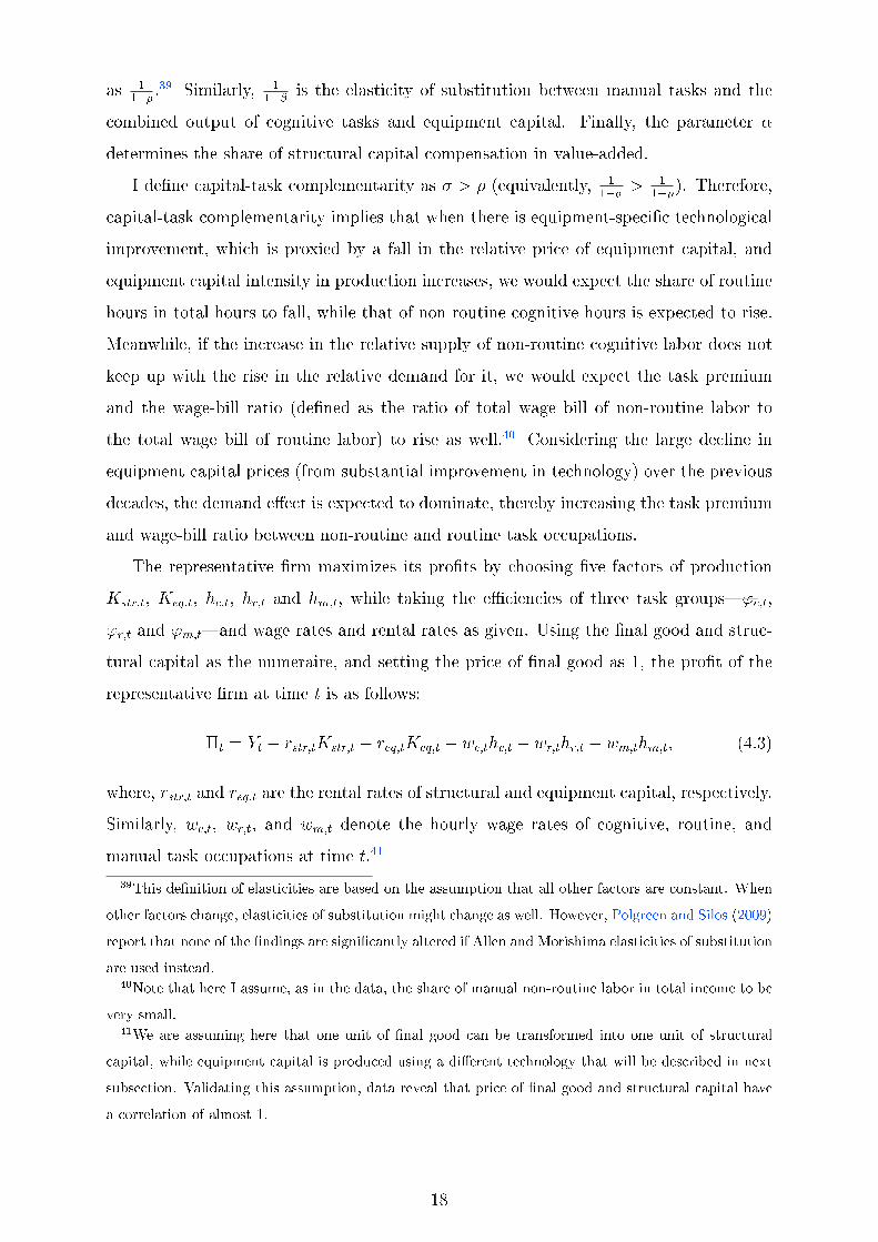
the labor share. The dotted blue lines showing model �t in panels (a) and (b) are plotted

with the assumption of zero shocks to the e�ciencies, and hence, they show the ability

of the model and observable covariates such as capital and hours series to account for

the changes in the data. As panel (a) implies, the model can account for most of the

rise in the task premium between cognitive and routine task occupations since the 1980s

but fails to fully capture the fall prior to that year. Panel (c), on the other hand, shows

the net rates of returns on two types of capital, which is obtained by rearranging the

no-arbitrage condition.

Figure 4.1: Model Targets: Data versus Model

Panels (a) and (b) are HP-trends. Panel (c) shows the expected rates of return on two types of

capital in model.

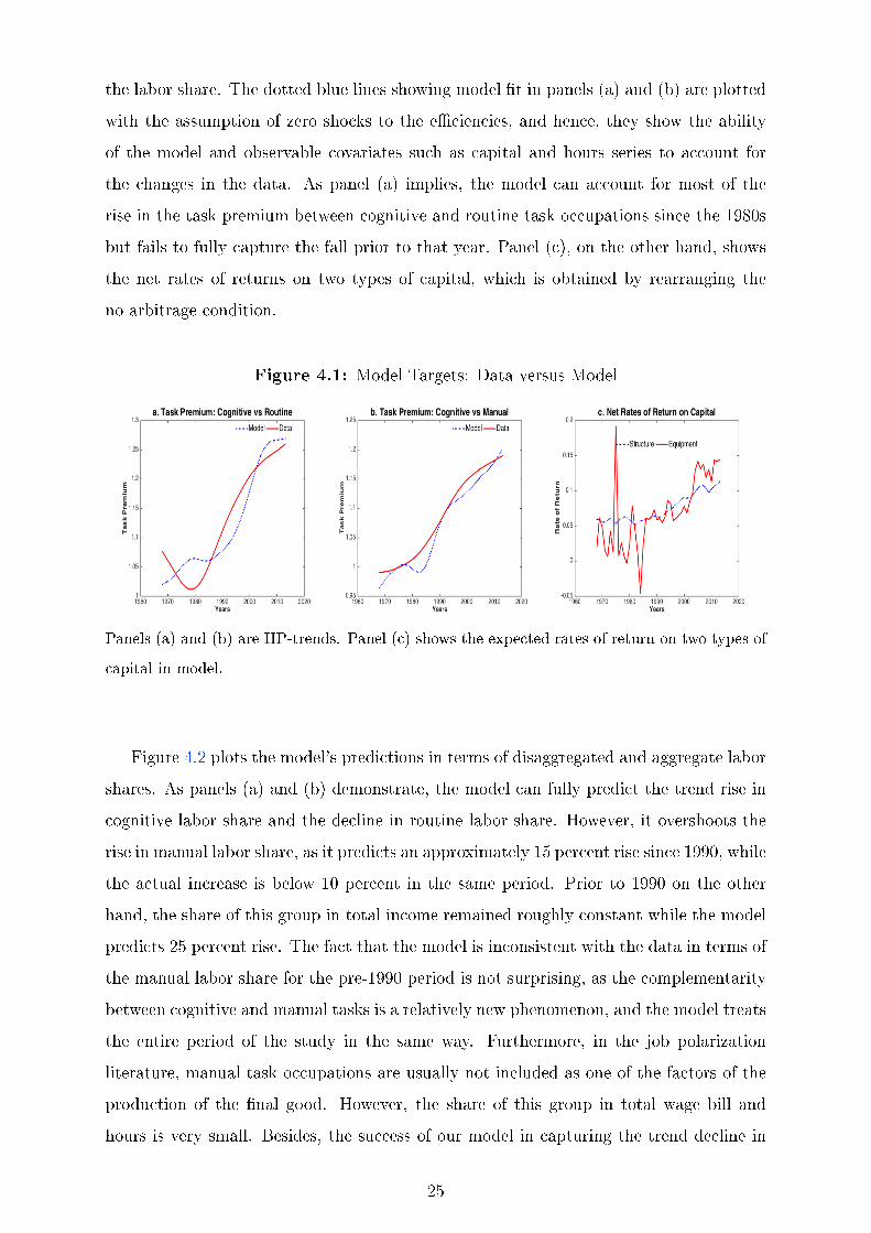
Figure 4.2 plots the model's predictions in terms of disaggregated and aggregate labor

shares. As panels (a) and (b) demonstrate, the model can fully predict the trend rise in

cognitive labor share and the decline in routine labor share. However, it overshoots the

rise in manual labor share, as it predicts an approximately 15 percent rise since 1990, while

the actual increase is below 10 percent in the same period. Prior to 1990 on the other

hand, the share of this group in total income remained roughly constant while the model

predicts 25 percent rise. The fact that the model is inconsistent with the data in terms of

the manual labor share for the pre-1990 period is not surprising, as the complementarity

between cognitive and manual tasks is a relatively new phenomenon, and the model treats

the entire period of the study in the same way. Furthermore, in the job polarization

literature, manual task occupations are usually not included as one of the factors of the

production of the �nal good. However, the share of this group in total wage bill and

hours is very small. Besides, the success of our model in capturing the trend decline in

25

the labor share stems from task-based de�nition, rather than inclusion of manual tasks

separately from cognitive non-routine tasks.48 Therefore, I prefer keeping the manual-

task as a part of the �nal good production for computational purposes; however, I de�ne

a second sector employing only manual task labor in the general equilibrium version of

the model.

Figure 4.2: Labor Shares: Data versus Model

The series are HP-trends.

Panel (d) of Figure 4.2 shows that a model describing the job and wage polarizations

can fully account for the trend decline in the aggregate labor share. At this point, the

reader might wonder whether the estimation strategy mechanically implies targeting the

labor share or not. In the end, we are targeting relative prices of types of labor and

feeding their quantities. Can this guarantee that the labor share trend will be captured

in any case? As Figure 4.3 depicts, the answer to this question turns out to be no. This

�gure shows the model-generated labor share when I estimate the model with the same

48The �t of the aggregate labor share signi�cantly improves when we switch from the education-based

skill classi�cation to the task-based classi�cation. On the other hand, when I estimate the model by

aggregating cognitive and manual tasks as \non-routine," the �t of the aggregate labor share is not

noticeably altered.

26

strategy but de�ne the skill on the basis of having a college degree or not. As in our

baseline estimation, I targeted the skill premium and the regular no-arbitrage condition,

thereby making the labor share an outcome of the model. Figure 4.3 shows that the

model is unable to foresee the decline in the aggregate labor share in the last decade.

During the entire period, the model predicted only around 58 percent decline in the labor

share, which proves that switching to the task-based skill de�nition signi�cantly improves

our understanding of the decline of the labor share.

Figure 4.3: Model's Prediction with Education-Based Skill Classi�cation

The series are HP-trends.

The dotted blue line shows the �t of the model when the labor is split as skilled and unskilled

on the basis of years of education.

4.4.2 Elasticities of substitution and shape of the production function

One of the goals of this paper is providing the elasticities of substitution that need

to be used in job polarization literature. The estimation results for the parameters

governing those elasticities are presented in Table 4.3. The elasticity of substitution

between equipment capital and labor devoted to routine tasks is measured as 2:40, while

equipment capital and labor employed in non-routine occupations are found to be neither

substitutes nor complements.49 Finally, as can be seen in the last column of Table 4.3,

49Even though not directly comparable due to di�erent classi�cations of labor, these elasticities are

stronger than the commonly used measures in the capital-skill complementarity literature. Krusell et al.

(2000) report the elasticity of substitution between equipment capital and unskilled labor, which is most

closely corresponds to our routine labor, as 1:67. Also, they estimate a strong complementarity between

27

Table 4.3: Estimation Results

� � �

Mean 0:5833 0:0240 0:0420

Mode 0:5930 �0:0044 0:0462

Standard Deviation 0:0160 0:0198 0:0252

Elasticity 2:40 1:02 1:04

there is neither strong complementarity nor substitutability between manual service tasks

and the composite of equipment capital and cognitive tasks, which is consistent with the

common view in the job polarization literature.

Signi�cance tests conducted at 95 percent con�dence level give p-values higher than

0:05 for the parameters � and �.50 In other words, the elasticities of substitution between

equipment capital and cognitive task and between manual tasks and the composite of

equipment capital and cognitive tasks are not signi�cantly di�erent from 1. This �nding

implies that we can model job/wage polarization and the labor share with a functional

form of production that has a Cobb-Douglas relationship between equipment capital,

the cognitive task and the manual task. In more aggregate terms, I document that the

production function is Cobb-Douglas between equipment capital and labor associated

with non-routine task occupations.

4.4.3 Implications

The partially Cobb-Douglas production function has important implications. First of all,

it shows that the neo-classical view of constancy of the labor share is still valid, albeit

at a smaller scale. Any part of the income that is lost by labor employed in routine task

occupations is proportionately captured by equipment capital and labor devoted to non-

routine tasks. This implies that the economy will converge to another steady state with

a constant but lower labor share once this transformation is completed. Second, as will

be formally proven in next subsection, with this Cobb-Douglas structure, the changes in

the labor share can be pinned down only to the changes in the composition of the wage

equipment capital and skilled labor, which can be considered as our cognitive labor. They estimate the

elasticity of substitution between these two factors as 0:67.50p-value reported for � is 0:2265 and for � is 0:0952. Here, the null hypotheses are � and � are

separately not di�erent from zero.

28

bill. To be more speci�c, the decline in the labor share can be explained and modeled by

capital-task complementarity that will distort the wage-bill ratio between non-routine and

routine tasks in favor of the non-routine labor following technological advances. In the

upcoming sections, I will introduce a simple general equilibrium model following from

this �nding and show that equipment-speci�c technological progress and capital-task

complementarity alone can account for most of the decline of the labor share. Finally,

using the Cobb-Douglas speci�cation signi�cantly reduces the burden of the estimation,

as we now have two less parameters to estimate.

Since the estimation of the general functional form indicates a Cobb-Douglas speci�-

cation instead of inner CES aggregators, we can use the following production function:

Y = AK�str

��L�r + (1� �)

�K eqL

�cL

1� ��m

��� 1��� : (4.14)

When I estimate the model using the production function speci�cation in equa-

tion 4.14, neither the model �t, nor the prediction of the model in terms of the labor

shares, is visibly altered. Figure A.4 replicates Figures 4.1 and 4.2 for the Cobb-Douglas

version of the model, and the reader can verify that the model �t does not worsen, if not

improve.

Table 4.4 reports the estimation outcome for the key parameters. The elasticity of

substitution between routine task and the composite of equipment capital and non-routine

tasks is 2:33, which is close to the value obtained for the general functional form. As

reported in the last column, 35 percent of the total income that is left after the compen-

sations of structural capital and the routine tasks are paid goes to equipment capital,

while the remaining 65 percent goes to labor employed in non-routine task occupations.

Hence, the 65 percent to 35 percent balance between labor and capital in neoclassical

theory turns out to be still valid at a smaller scale than the aggregate economy.

Table 4.4: Estimation Results for the Cobb-Douglas Speci�cation

� �

Mean 0:5708 0:5566 0:3528

Mode 0:5610 0:5530 0:3567

Standard Deviation 0:0057 0:0198 0:0066

Elasticity 2:33 - -

29

4.4.4 Labor share in the model

The production function in equation 4.14 yields the following labor share equation:

LSt = (1� �)�L�r;t + (1� �)(1� )K�

eq;tL��c;tL

�(1��� )m;t�

�L�r;t + (1� �)hK eq;tL

�c;tL

1��� m;t

i�� : (4.15)

When this equation is rearranged, details of which can be found in equations C.11-C.18 in

Appendix C, I obtain the following relationship between the labor share and the wage-bill

ratio between non-routine and routine tasks:

LSt = (1� �)1 + wbrt

1 + wbrt1�

: (4.16)

In growth terms,51 cLSt = �dwbrt "

wbrt + (2� ) + (1� )wbrt

#; (4.17)

where, the growth rate of the wage-bill ratio between non-routine and routine tasks is

given as: dwbrt = �h�cLct + dKeqt + (1� � � )cLmt �cLrti : (4.18)

Equation 4.17 reduces the growth rate of the labor share down only to the negative

of the growth rate of the wage-bill ratio and a key parameter , which is the weight of

equipment capital in Cobb-Douglas segment of the production function. The wage-bill

ratio, on the other hand, rises faster if (i) the possibilities to switch from routine task

to non-routine tasks and equipment capital are higher and (ii) the cost function is more

sensitive to the changes in equipment capital prices. The former condition corresponds to

a larger elasticity of substitution between routine task and composite output of equipment

capital and non-routine tasks, while the latter corresponds to a larger weight of equipment

capital ( ) in the Cobb-Douglas speci�cation.52

Equation 4.17 shows that anything that will raise the wage-bill ratio in favor of non-

routine labor will cause a decline in the labor share as well. Thus, in an environment

where price of equipment capital declines rapidly, capital-task complementarity with unit

elasticity between equipment capital and non-routine labor is su�cient to distort the

wage-bill ratio in favor the labor working in non-routine task occupations, thereby causing

51Steps of converting equation 4.16 into growth terms are presented in equations C.19-C.25.52Note that this former condition is also equivalent to having a larger capital-task complementarity,

which is measured by � in our case, as the parameter governing the elasticity of substitution between

non-routine tasks and equipment capital is documented to be zero. Hence, ��0 = � is at the same time

our capital-task complementarity measure.

30

a decline in the labor share. Nonetheless, the e�ect of the rise in the wage-bill ratio on

the labor share decreases over time, even if the wage-bill ratio continues to grow. This

can be seen from the second term in equation 4.17: Dt =

wbrt+(2� )+(1� )wbrt

. The term Dt

�rst rises in wbrt and then starts falling as wbrt passes a certain threshold, as shown in

Figure A.5. The reverse U-shape of the coe�cient Dt strengthens our conjecture that the

U.S. economy is currently at early stages of a long-term transition period that is likely

to cool down in the medium-term, even if the composition of the wage bill continues to

change at its current pace.

4.4.5 Testing the estimation outcome using the aggregate and sectoral data

If the functional form estimated is correct, we should be able to replicate the decline of

the labor share by feeding equation 4.17 with the wage-bill ratio series calculated from

the CPS data. Figure 4.4 plots the model �t obtained from this exercise. It is clear from

the �gure that the wage-bill ratio series can account for almost all of the trend decline of

the labor share in the long run.53

A similar exercise is repeated for some selected sectors. To do so, I �rst calibrate s

for each sector.54 Then, I feed equation 4.17 with the sectoral wage-bill ratios. As panels

(a) and (b) of Figure A.6 show, the wage-bill ratio does remarkably well in replicating

the decline in labor shares in some sectors such as Food, Tobacco and Beverages, and

Finance and Insurance. However, as panels (c) and (d) depict, equation 4.17 fails to fully

explain why the labor share rises in some of the sectors; yet, it does not predict a fall

in these sectors either. This failure most probably stems from ruling out other sector-

speci�c factors, such as an increase in relative demand for those sectors or heterogeneity

in sector-speci�c technological progresses or substitution possibilities. The success of the

model for other sectors lies somewhere between these two extremes. Considering that I

assumed same substitutability at each sector, the model's predictions of the labor share

53It should be reminded here that this paper views the changes in the labor share from a long-term

perspective. Thus, the model does not capture short term cyclical or trend changes in the labor share.54To calibrate sector speci�c s, I �rst calculate the wage-bill of labor employed in non-routine task

occupations from the CPS data. Then I use the ratio of this to total wage bill as the weight of this

group in the aggregate labor share. Multiplying this weight by the labor share of this sector in EU-

KLEMS data set gives me income share of labor devoted to non-routine tasks in that sector. The share

of equipment capital is also calculated from the EU-KLEMS data set. is then obtained as the ratio of

the equipment capital compensation share to the sum of the compensation shares of equipment capital

and labor associated with non-routine tasks.

31

should be considered as a lower bound of our ability to explain the labor share trends by

equipment-speci�c technological change and capital-task complementarity.

Figure 4.4: Labor Share Fit, by Wage-Bill Ratio Series Alone

The series are HP-trends.

The dotted blue line is generated by feeding equation 4.17 with the wage-bill ratio series calcu-

lated from the CPS data and using the parameter = 0:3528.

Being able to replicate the labor share trend based only on the wage-bill ratio series

and a single parameter signi�cantly reduces the burden of the analysis. To be more spe-

ci�c, we do not need to make assumptions about a whole set of capital stocks and prices

and labor input series if we want to predict the future path of the labor share. For in-

stance, if we assume that the wage-bill ratio continues to grow at its current average rate

of 2 percent per year, equation 4.17 tells us that the labor share should stabilize around

55 percent. Sole dependence of the labor share on the wage-bill ratio also simpli�es the

general equilibrium model that I will use to quantify the decline of the labor share that

can be attributed to equipment-speci�c technological progress and capital-task comple-

mentarity. As long as we have the correct elasticity of substitution between routine jobs

and other factors of production, and a correct weight of equipment capital in the Cobb-

Douglas speci�cation, the decline in relative equipment capital price will be su�cient to

raise the wage-bill ratio in favor of labor working in non-routine task occupations. The

rise in the wage-bill ratio, in turn, is expected to generate a trend decline in the labor

share at a magnitude similar to the data if the model parameters are well identi�ed.

Before proceeding to the general equilibrium model, I test the key mechanism implied

by the estimation using the sectoral data. Figure 4.5 shows that for a given level of

32

elasticity of substitution between routine task and composite output of equipment capital

and non-routine tasks, in sectors for which the weight of equipment capital compensation

in the Cobb-Douglas speci�cation is larger, the rise in the wage-bill ratio is larger as

well. The weighted coe�cient of correlation between the annual trend change of the

wage-bill ratio and the parameter is 0:67 and signi�cant with a p-value of almost 0.

Figure 3.4, which was presented earlier, on the other hand, con�rms the remaining part

of the mechanism: in sectors where the wage-bill ratio rose more, the trend decline of

the labor share was larger as well. To sum up, considering that we ruled out possible

di�erences in elasticities of substitution across sectors, the estimated aggregate production

function and the implied key channel driving the labor share trend does remarkably well

in explaining di�erences across sectors as well.

Figure 4.5: Weights of Equipment Capital and Wage-Bill Ratios across Sectors

Trend coe�cients are obtained from regressions of log series on a constant and a time variable.

5 General Equilibrium Model

The estimation analyses have provided us with two important ingredients for modeling

the decline of the labor share. First, it gave us the shape of production function that is

consistent with major employment and wage shifts observed over the past few decades

as well as the decline in the labor share. Second, and more importantly, it revealed that

we can model the labor share decline by a rise in the wage-bill ratio, which is triggered

by technological advances and capital-task complementarity. Up until now, all of the

33

variables of the model were exogenous in our analysis. From now on, I will only keep

technological change as exogenous and all the remaining variables will be determined en-

dogenously within a dynamic general equilibrium environment. This way, we can quantify

part of the labor share trend that can be accounted for by the decline in relative equip-

ment capital prices only. This model can also be used for conducting counterfactual

exercises, labor share projections, and policy analysis.

5.1 Model Environment

The household sector consists of two types of agents: skilled and unskilled. The repre-

sentative household of each type has a continuum measure of unit 1 individuals di�ering

in their routine task e�ciencies. The representative households supply their labor inelas-

tically and, taking the wages as given, assign their members to occupations. Members of

the skilled household can work in either cognitive or routine task occupations, while the

unskilled household makes a choice between routine and manual task occupations. Cog-

nitive and routine hours in e�ciency are combined with both structural and equipment

capital to produce the �nal good that is consumed and invested. In addition, there also

exists a sector producing manual services by employing only labor for manual tasks.55

Finally, technological progress enters the model exogenously in the form of a rise in the

productivity of equipment capital-speci�c production.

5.2 The Households' Labor Supply and Investment Decisions

There is a measure of S skilled and a measure of U unskilled households in the economy.

Both types of agents face similar problems in the sense that they assign their members

into occupations and save an asset that is used in purchasing both types of capital.

However, each type of agent di�ers in a couple of dimensions. First, members of the

skilled household do not have access to the manual labor market, while the unskilled

agents cannot be employed in cognitive task occupations.56 On the other hand, both

types can work in routine task occupations. Secondly, manual services are assumed to

be consumed only by the skilled agents. This assumption is consistent with the proposed

55The manual services in the model represent the personal services such as child care, cleaning, and

home health care.56Even if the skilled agents were allowed to work in manual task occupations, they wouldn't prefer

doing so unless manual sector wages are too high. Thus, the set-up is simpli�ed by ruling out the manual

employment of the members of the skilled household.

34

relationship between cognitive task labor and manual services in the job polarization

literature. Yet, this is a trivial assumption and does not a�ect the quantitative �ndings

of the paper.

5.2.1 Problem of the skilled agent

The skilled household has members with the vector of e�ciencies (�; �i; 0) for cognitive,

routine, and manual task occupations respectively. In other words, skilled individuals

have access to two labor markets. If they work in cognitive task occupations, their

e�ciency is �, and thus they receive an hourly wage rate of �wc;t, where wc;t is the wage

rate for cognitive task occupations. Alternatively, they can prefer working in routine

task occupations. Their e�ciencies in routine task occupations are ranked by �i, which

is assumed to be distributed uniformly between 0 and 1: �i � U [0; 1]. These identi�ers

are translated into routine task e�ciencies through the function h(�i). Thus, the skilled

individuals working in routine task occupations receive e�ciency wages equivalent to

h(�i)wr;t, where wr;t is the wage rate for these occupations.57 Following Beaudry et al.

(2013), I choose h(�i) = �� 1

2i as the functional form of routine task e�ciency.

The skilled household consumes a composite of �nal good and manual services; save

an asset and chooses a cuto� ��t that determines the allocation of its members between

occupations. The household's inter-temporal problem is:

maxcs;g;t;cs;m;t;as;t+1;��t

E

"1Xt=0

�tlog(cs;t)

#;

subject to

cs;g;t + pm;tcs;m;t + zas;t+1 � wc;t

Z 1

��t

�d� + wr;t

Z ��t

0

h(�i)d� +Rtas;t: (5.1)

Here, cs;g;t and cs;m;t are the skilled household's consumption of �nal good and manual

services, respectively. as;t+1 is the household's assets at time t + 1, while Rt is the gross

return on the asset between periods t and t + 1. z, on the other hand, is a common

growth factor, used in de-trending the variables, and � is the discount factor. Finally,

cs;t is the composite consumption of the skilled household, such that

cs;t =��c�s;g;t + (1� �)c�s;m;t

� 1� ; (5.2)

57Instead of allowing the members of the skilled household di�er in their cognitive task e�ciencies, I

preferred the current set-up for modeling purposes. Thus, having a high routine task e�ciency can be

considered as having comparative advantage in routine tasks. Therefore, from a reverse perspective, these

members of the skilled group can be thought of as having a comparative disadvantage in occupations

requiring cognitive skills.

35

where, the demand elasticity of substitution between �nal good and manual services is

11��

.

Utility maximization requires that the marginal utility per dollar should be equalized

between the �nal good and manual services consumptions:

pm;t =1� �

�

�cs;g;t

cs;m;t

�1��

: (5.3)

The �rst order condition with respect to ��t gives us the rule for cuto� e�ciency rank as

shown below:wc;t

wr;t=

��t� 1

2

�: (5.4)

.

Equation 5.4 shows that the member of the household with e�ciency rank ��t will

be indi�erent between working in cognitive and routine task occupations. The members

with e�ciency rank above ��t, on the other hand, will supply their labor endowment to

occupations associated with cognitive tasks. When the advances in technology raises the

relative wage of cognitive task occupations, cuto� e�ciency rank will fall, and thus more

skilled labor will be employed in these occupations.

Finally, we have the usual Euler equation that makes the skilled household indi�erent

between consuming one more unit today and saving that one unit and consuming it in

the next period:

c��1s;g;t

c�s;t z = �Et

"c��1s;g;t+1

c�s;t+1Rt+1

#: (5.5)

5.2.2 Problem of the unskilled agent

The problem of the unskilled household is similar. The unskilled household has members

with the vector of e�ciencies (0; i; 1) for cognitive, routine, and manual task occupations,

respectively. Thus, unlike the skilled agent, the unskilled does not have access to the labor

market for cognitive occupations. However, it competes with the skilled agents for the

routine task occupations. The members of the household are uniformly ranked between

0 and 1. Their rank, i, determines their e�ciency in routine task occupations. Similar

to the skilled agents, these identi�ers are translated into routine task e�ciencies through

the function g( i). As before, I assume that the e�ciency is decreasing in i, meaning

that g( 0i) < 0. However, it is assumed, on average, that the routine task e�ciency of the

unskilled labor is lower than that of skilled labor. In particular, I specify that for each

rank level i = �i, g( i) = bh(�i), where 0 � b � 1. Thus, the unskilled individuals doing

routine tasks receive g( i)wr;t worth of e�ciency wage. The members of the unskilled

36

household also have the option of supplying their labor endowments to manual service

production, where the wage rate is wm;t. Comparing these two wage rates in e�ciency

units, the household chooses an e�ciency rank cuto� that determines the fraction of its

members assigned to routine and manual task occupations.

The unskilled household consumes only the �nal good, and, similar to the skilled

agent, it saves an asset and chooses a cuto� � t that determines the allocation of its

individuals between tasks. The household's inter-temporal problem is:

maxcu;g;t;au;t+1; � t

E

"1Xt=0

�tlog(cu;g;t)

#;

subject to

cu;g;t + zau;t+1 � wr;t

Z � t

0

g( i)d + wm;t

Z 1

� t

1d +Rtau;t; (5.6)

where, cu;g;t is the unskilled household's consumption of �nal good, au;t+1 is its asset

holdings at the end of period t, and � t is the e�ciency rank cuto� that determines the

allocation of members of the household across occupations. This cuto� is determined by

the �rst order condition with respect to � t. When there is technological advancement, the

demand for cognitive tasks is expected to rise, which, in turn, will raise the total income

of the skilled group. As they are the sole demanders of manual services, the demand and

relative price of these services will rise. Hence, wage paid to manual task occupation will

rise relative to the occupations associated with routine tasks, and, as equation 5.7 shows,

this will raise the cuto�, leaving less unskilled workers in routine task occupations.

wm;t

wr;t= b �

� 12

t (5.7)

Finally, we have our usual Euler equation coming from the agent's inter-temporal saving

decisions:1

cu;g;t z = �Et

�1

cu;g;t+1Rt+1

�: (5.8)

5.3 Final Good Production

The representative �rm produces the �nal good that is either consumed or invested in

either structural or equipment capital. The �nal good Yg is produced using four factors of

production: structural capital (Kstr), equipment capital (Keq), cognitive (Lc), and routine

task (Lr) hours in e�ciency units. Consistent with the estimation outcome, there is a

Cobb-Douglas relationship between equipment capital and cognitive task, while there

is non-unitary elasticity of substitution between the composite of these two factors and

37

routine task:

Yg;t = AtK�str;t

��L�r;t + (1� �)L

(1� )�c;t K

�eq;t

� 1���

; (5.9)

where, At is the total factor productivity (tfp) term, for which the following stochastic

process is de�ned:58

lnAt = �A lnAt�1 + �A;t:

The �nal good is chosen as the numeraire, and thus its price is set as 1. The rep-

resentative �rm takes the wages and rental rates of capitals as given and maximizes its

pro�ts by choosing quantities of four factors of production. The problem of the �rm at

time t is described as:

maxKstr;t;Keq;t;Lc;t;Lr;t

Yg;t � wc;tLc;t � wr;tLr;t � rstr;tKstr;t � req;tKeq;t:

The �rm's optimal decision rules are given by the following �rst order conditions:

wc;t = (1� �)(1� �)(1� )Yg;t

�L�r;t + (1� �)L(1� )�c;t K

�eq;t

K �e;tL

(1� )��1c;t (5.10)

wr;t = (1� �)�Yg;t

�L�r;t + (1� �)L(1� )�c;t K

�eq;t

L��1r;t (5.11)

req;t = (1� �)(1� �) Yg;t

�L�r;t + (1� �)L(1� )�c;t K

�eq;t

K ��1eq;t L

(1� )�c;t (5.12)

rstr;t = �Yg;t

Kstr;t: (5.13)

5.4 Personal (Manual) Services Production

The manual services sector represents the home production. This sector is essential, as

it helps the model generate a larger decline in labor devoted to routine tasks in the re-

sponse to declining demand for this type of labor following the fall in equipment capital

prices. In the job polarization literature, manual task occupations are neither comple-

ments nor substitutes to equipment capital. However, equipment capital and manual task

occupations are indirectly linked through the consumption behavior of labor employed

in cognitive task occupations. As demand for these high-skill types of task rises, their

income rises as well, which, in turn, increases the demand for manual services by labor

employed in cognitive task occupations. Therefore, the share of labor devoted to manual

tasks in total income and hours shows a modest rise.

58This tfp process will be fed with the shocks, which I obtain from the estimation process, when solving

for the general equilibrium model under perfect foresight.

38

Consistent with the job polarization literature, including Autor and Dorn (2013), the

production function for manual services is assumed to be linear. To be more speci�c, one

unit of manual labor input produces one unit of manual services:

Ym;t = Lm: (5.14)

Letting pm denote the price of one unit of manual service and wm the hourly wage rate

in this market, pro�t maximization under perfect competition yields:

pm = wm: (5.15)

5.5 Technological Progress

The �nal good is either consumed or invested in structural or equipment capital. One unit

of investment in structural capital is converted into one unit of this type of capital. On the

other hand, investment in equipment capital is scaled by a factor qt before being added to

equipment capital stock. qt here represents the equipment-speci�c technological progress

and will be assumed to be exogenous in the model. As it had already been discussed in

the estimation part, perfect competition drives the relative price of equipment capital to:

peq;t =1

qt: (5.16)

5.6 Equilibrium

For a given level of equipment-speci�c technology qt, an equilibrium for our model econ-

omy is a collection of prices fwc;t; wr;t; wm;t; rs;t; re;t; Rt; pm;t; peq;tg, capital stocks and

assets fKstr;t; Keq;t; as;t; au;tg, quantities of consumption and output fYg;t; Ym;t; cs;t; cs;g;t;

cs;m;t; cu;g;tg, labor hours in e�ciency units fLc;t; Lr;t; Lm;tg, and e�ciency rank cuto�s

f��t; � tg such that: (1) households maximize their discounted utilities subject to their

budget constraints, (2) both the �nal good producers and manual service producers max-

imize their pro�ts, (3) labor markets clear:

Lc;t =

Z 1

��t

�d�S = (1� ��t)�S (5.17)

Lr;t =

Z ��t

0

��1=2i d�S + b

Z � t

0

�1=2i d U = 2��

12t S + 2b �

12t U (5.18)

Lm;t =

Z 1

� t

1d U = (1� � t)U; (5.19)

39

(4) capital and asset markets clear:

as;tS + au;tU = Kstr;t + ptKeq;t (5.20)

peq;t+1

peq;t=

1

1� �eq

�rstr;t+1 + (1� �str)�

req;t+1

peq;t

�(5.21)

Rt = 1� �str + rstr;t; (5.22)

and (5) manual service market clears:

cs;m;tS = Ym;t: (5.23)

Households invest in one type of asset, which is then purchased by a zero-pro�t inter-

mediary and converted into two types of capital. Thus, market clearing requires that the

total amount of savings should be equal to the total value of the capital (equation 5.20).

The intermediary's investment decision will be such that the expected return on two

types of capital should be equal (equation 5.21). Otherwise, there would be investment

in only one type of capital in the model economy. Finally, gross returns on the asset and

each type of capital should be equalized as well (equation 5.22).

In summary, there are 23 unknowns in our model fwc;t; wr;t; wm;t; rs;t; re;t; Rt; pm;t; peq;t;

Kstr;t; Keq;t; as;t; au;t; Yg;t; Ym;t; cs;t; cs;g;t; cs;m;t; cu;g;t; Lc;t; Lr;t; Lm;t; ��t; � tg, and all 23 equa-

tions between 5.1 and 5.23 solve for these unknowns.

6 Quantitative Analysis

In this section, the general equilibrium model introduced above is used to quantify the

contribution of the equipment-speci�c technological progress to the trend decline in the

labor share. First, I discuss the parameterization of the model. Later, I brie y present

the solution method and report the model's �ndings. Finally, I discuss the implications

of the model for heterogeneity in labor share trends across sectors.

6.1 Parameterization

The model parameters are set in three main blocks: estimation, regression, and calibra-

tion. Below, I describe each of these in detail. The reader can refer to Table B.2 in

Appendix B, which lists all the parameters of the model and the sources of parameteri-

zation.

40

6.1.1 Estimation

The �rst set of parameters are already available from the estimation part in Section 4. In

particular, � = 0:5708, which is the parameter that governs the elasticity of substitution

between labor employed in routine task occupations and the composite output of equip-

ment capital and non-routine tasks. This value of � implies an elasticity of substitution

of 2:33. Furthermore, the choice of production function in equation 5.9 is based on the

estimation result that equipment capital and cognitive tasks are neither complements, nor

substitutes. Finally, I borrow the parameter , which is the share of equipment capital

in the partial Cobb-Douglas speci�cation between equipment capital and cognitive task,

from Table 4.4.59

6.1.2 Regression

There are two parameters in the CES consumption aggregator in equation 5.2: � is the

parameter that shapes the elasticity of substitution between consumption of the �nal good

and manual services. The other parameter, �, is the share of the �nal good in aggregate

consumption of the skilled agent. To recover these two parameters, I combine the �rst

order conditions of the skilled household with respect to each types of consumption, which

gives:

pm;t =1� �

�

�cs;g;t

cs;s;t

�1��

:

Then, I take the logarithm of this equation and run the following simple regression:

ln pm;t = ln1� �

�+ (1� �) ln

�cs;g;t

cs;s;t

�+ ut:

In this regression, I use personal consumption of goods and services (apart from the

\other services" category) from NIPA Table 2.3.6 as consumption of the �nal good in

our model, cs;g;t, and personal consumption expenditures on other services as manual

services, cs;m;t. The price series, on the other hand, are taken from NIPA Table 2.3.4 for

the 1967{2013 period. This regression gives us � = 0:9410 and � = �0:1547. This level

of � corresponds to an elasticity of substitution between �nal good and manual services

equal to 0:87, which implies complementarity between these two consumption items.

59However, here an adjustment is needed since the production function for the �nal good in general

equilibrium model does not encompass manual tasks. Thus, I distribute the share of labor employed in

manual task occupations reported in Table 4.4 proportionally to equipment capital and labor devoted to

cognitive task occupations, which gives us = 0:3879.

41

6.1.3 Calibration

Data: Some parameters are taken directly from the data. To begin with, depreciation

rates for each type of capital are easily recoverable from NIPA �xed assets tables. For

the entire period 1967{2013 period, I divide the consumption of capital series from Table

2.4 by the capital stock series from Table 2.1. The average depreciation rates found are

�s = 0:0275 for structural capital and �e = 0:1460 for equipment capital. Furthermore,

discount rate � is taken as 0:96 to match approximately 4 percent annual interest rate

in equilibrium. Measure of the unskilled agents is normalized as 1. Then I calculate the

average share of hours worked by college and above educated labor in total hours from the

CPS data set for the 1967{2013 period, which gives S = 0:361. Finally, z, the common

growth factor, is set equal to the growth rate of the total factor productivity obtained as

a residual from the estimation in Section 4.

Targeting initial values: There remain four parameters to calibrate: � is the share

of routine task occupations in CES between routine task occupations and the composite

of equipment capital and cognitive task occupations as in production function in equa-

tion 5.9; b is the scale parameter between the routine task e�ciencies of the skilled and

the unskilled agents; � is the cognitive task e�ciency of the skilled household; and peq;0

is the initial relative price of equipment capital. To set these parameters, I set year 1966

as the initial steady state and target levels of some of the key variables in that year. To

be more speci�c, I target the wage-bill ratio between cognitive and routine tasks in 1966

to recover �. To obtain two e�ciency parameters, I target the task premiums. Finally,

the ratio of real equipment capital stock to real structural capital stock gives us peq;0.

These targets are shown in the left two columns of Table 6.1. The right two columns, on

the other hand, show the data and model levels of other selected variables for the initial

year.

These targets give us � = 0:4160, � = 1:8681, b = 0:6493, and peq;0 = 0:8302.

6.2 Perfect Foresight Solution

It is well known in the literature that models with capital-augmenting technological

growth do not have balanced growth path properties. Therefore, I rule out the growth in

equipment-speci�c technology and de�ne a random-walk process for it, thereby making

every technology shock persistent. Hence, following each shock to the equipment-speci�c

technology, the economy moves towards a potentially new steady state over time.

42

Table 6.1: Targets and Other Selected Moments for 1966

Data Model Data Model

Targeted Not Targeted

wbrcr 0:58 0:58 LSagg 0:70 0:73

tpcr 1:46 1:46 LScog 0:24 0:26

tpmr 0:70 0:70 LSrtn 0:41 0:45

Keq

Kstr0:78 0:78 LSman 0:05 0:03

wbrmr 0:11 0:10

I solve the model under perfect foresight assumption. In other words, I assume that

at the beginning of the �rst period, agents are fully aware of future paths of qt and

shocks to the total factor productivity. This solution method requires imposing initial

and terminal conditions and solving the path from one to the other. To do so, I assume

that the relative equipment capital price was constant up to year 1966 at its price in

this year. Then, the year 1966 is imposed as the initial steady state. Later, agents are

assumed to learn the future path of both technology and total factor productivity shocks

beginning from 1967. In the baseline scenario, I assume that equipment capital-speci�c

technology stays constant at its 2013 level and the economy reaches its new steady state

at this level of technology T periods after this. Then, I solve 23 � (T + 47) equations

simultaneously.60

6.3 Findings

The paths of the key variables under the perfect foresight solution are presented in Fig-

ure 6.1. The three �gures in the top row show the labor share trends for three task

groups. Both panels (a) and (b) show that the task-based explanation for the trend

decline in the labor share is quite successful for labor employed in cognitive and routine

task occupations for the period after 1990. However, in the �rst half of the period of

study, the model can account for only around 40 percent of the trend changes in these

labor shares. Furthermore, even though the model is unable to capture the large cycles

observed in the data, it successfully captures the total rise in the income share of labor

60I tried various T s ranging from 50 to 500 periods to check if the choice of the terminal year a�ects

the results. Fortunately, there was no noticeable di�erences in results for di�erent choices of T s in this

range.

43

associated with manual tasks as depicted in panel (c) of the Figure 6.1.

Consistent with the task-level labor shares, the model's success in predicting the

aggregate labor share is di�erent in the �rst and second halves of our period of study.

As panel (d) of Figure 6.1 shows, 87 percent of the labor share trend after 1990 can be

explained by the advances in equipment-speci�c technology. Up to year 1990, on the

other hand, we can attribute only 45 percent of the decline to this channel. Overall,

for the entire period 1967{2013 period, we can account for 72:2 percent of the trend

decline in the labor share by equipment-speci�c technological progress and capital-task

complementarity.

The model's performance in predicting the paths of the wage-bill ratios between var-

ious tasks groups is similar to the labor shares (panels (e) and (f) of Figure 6.1). This

is not a surprising outcome, as the advances in technology a�ect the labor share through

changes in the wage-bill ratio in my model. However, the model foresees a substantially

larger growth in task premiums, especially between cognitive and routine tasks, than

what we observe in the data. This overshooting of the task premiums results from the

assumption of exogenous (and �xed measures) of skill groups. My model does not allow

for skill accumulation, and hence, the measures of the skilled and the unskilled agents

are �xed at some pre-given levels. Normally, when there is technological progress and

capital-task complementarity, and thus, the demand for cognitive tasks rises, we would

expect to see both a rise in relative wage and also, over time, rise in total supply of skilled

agents, who are the sole suppliers of the cognitive hours. However, because the skill sup-

ply channel is shut o� in our model, the rise in the wage-bill ratio mostly stems from the

rise in the task premium, rather than a combination of relative hours and wages.61

6.3.1 Counterfactual: the e�ect of the technological boom on labor share

trend

The model's inability to fully account for the decline in the labor share for the pre-1990

period is consistent with the data. As discussed earlier, the between-sector component

was the dominant factor in this period, and my model does not allow structural shifts.

On the other hand, most of the decline in the labor share is due to the within-sectoral

changes for the post-1990 period. As a matter of fact, during the eight years between

1996 and 2003, the growth rate of technological progress has doubled (Table 6.2). This

61Incorporating a simple educational choice, like in Orak (2013), into the baseline model would poten-

tially eliminate the overshooting of the task premium.

44

Figure 6.1: Prefect Foresight Solution: Data versus Model

The series are HP-trends.

technological boom has been followed by an acceleration of the decline in the labor share.

As this is consistent with the proposed channel in my model, its performance in explaining

the labor share trend is substantially stronger for this period.

The model enables us to quantify the contribution of this technological boom alone on

the labor share trend. To do so, as depicted in panel (a) of Figure 6.2, for the 1996{2003

period, I �xed the growth rate of the relative equipment capital price at its average level.

Panel (b) of Figure 6.2 shows that the labor share would have been around 2 points higher

today if we had not had the technological boom of 1996{2003. These 2 points correspond

to about 22 percent of the decline in the labor share.

45

Table 6.2: Annual Growth Rate of Relative Equipment Capital Prices

Period Growth Rate

1967{1995 �:0342

1996{2003 �:0759

2004{2013 �:0378

1967{2013 �:0424

Figure 6.2: Counterfactual: the E�ect of the Technological Boom on the Labor Share

The labor share series in panel (b) are HP-trends.

6.3.2 Projection of the labor share

My model has a unique prediction for the future path of the labor share. The studies

relating the decline in the labor share to the substitutability between aggregate capital

and labor, such as Karabarbounis and Neiman (2014b), imply that the labor share should

converge to 0 over time if technological progress continues at its ongoing pace. However,

this paper documents that there is a speci�c group of labor that is losing due to tech-

nological progress, and a constant share of their losses is captured by the other group of

labor. Thus, the explanation proposed in this paper foresees a stabilization of the labor

share in the long run as the economy completes its transition to a new steady state with

a very low share of the labor employed in occupations associated with routine tasks.

To visualize this convergence to a new economy with lower but stable labor share, I

analyze how the labor share would respond to a 1 percent positive shock to equipment-

speci�c technology at various stages of technological progress. To do so, I impose a level of

technology for each year after 2013 based on the assumption that the relative equipment

capital price would continue to decline at its current average annual rate of 4:24 percent

46

for another 200 years. Then, I independently give a 1 percent technological shock at each

level and plot the impulse responses of the labor share to these shocks at various years.62

Each line in Figure 6.3 corresponds to the response of the labor share to a 1 percent

technological shock at the level of equipment-speci�c technology in the speci�ed year. As

the �gure depicts, the e�ect of technological progress on the labor share gradually fades

,even if technological progress maintains its strength.

Figure 6.3: Impulse Response of the Labor Share to a 1 percent Technological Shock

To project a lower bound for the U.S. labor share, I use the imposed future path

for the relative equipment capital price and solve the model under the perfect foresight

assumption. Even under this extreme case, the model predicts that the labor share will

stabilize around 55 percent in the long run, as Figure 6.4 shows. However, this number

should be interpreted with caution, as the nature of technological progress might evolve

over time, and what we de�ne as routine might drastically change.

6.4 Sectoral Decomposition

As discussed earlier, there has been substantial heterogeneity in the labor share trends

across sectors (Figure 3.3). Most of the goods sectors, including the manufacturing

industries, have experienced large trend decline in the labor share, while service sectors

62To solve for the stochastic version of the model, I de�ned a random-walk process for the equipment-

speci�c technology. Thus, each shock to the technology is permanent and the economy slowly moves to

a new steady state after the shock. It should be clari�ed at this point that each shock is given separately

for each year under the assumption that the economy is at the steady state before the shock.

47

Figure 6.4: Projection of the Labor Share

The series are HP-trends.

have shown a limited decline, if not a rise. How consistent is the sectoral experience

with our technological process and capital-task complementarity story? In the end, all

the sectors have faced similar equipment-speci�c technological progress. Likewise, task

premiums between various tasks have been rising at similar magnitudes in most of the

sectors. If sectors were to operate under same technology, we would expect the labor

shares to exhibit similar trends across sectors as well.

Two papers try to provide an explanation for this heterogeneity in labor share trends

across sectors. Orak (2015) shows that if the elasticities of substitution, and hence the

degrees of capital-task complementarity, are allowed to di�er across sectors, we can ac-

count for trend di�erences in the labor shares across sectors. Similarly, in their recent

paper, Alvarez-Cuadrado et al. (2015) claim that di�erences in the degree of aggregate

capital-labor substitutability across sectors can explain the decline in the sectoral and

aggregate labor shares. However, a three-sector extension of our model shows that we

can mimic the sectoral di�erences in the labor share trends even when the elasticities

between equipment capital and various types of labor are the same across sectors. In

other words, our key channel working through the rise in the wage-bill ratio is consistent

with the sectoral experiences as well, and this consistency does not rely on heterogene-

ity in the capital-task complementarities. The only factor that causes sectors to react

di�erently to technological change is the share of equipment capital in the partial Cobb-

Douglas speci�cation. When the extended model is calibrated to the U.S. data, I show

that in sectors where the share of equipment capital is larger (such as manufacturing),

48

advances in technology cause a larger rise in equipment capital per e�ciency hour and in

the wage-bill ratio between labor devoted to cognitive and routine tasks, thereby leading

to a larger fall in the labor share.

6.4.1 Extended Model

The problem of the households is the same as in the baseline model and thus is not

presented again. Furthermore, the manual service sector is kept as before as well. The

key di�erence between baseline model and the extended model is the introduction of two

intermediate outputs that are aggregated into our �nal good used in consumption and

investment. The production functions for these intermediate sectors are similar except

for three parameters that will be calibrated.

Intermediate sectors: Each intermediate sector i 2 f1; 2g has the following pro-

duction function:

Yg;i;t = AtK�istr;i;t

��iL

�r;i;t + (1� �i)L

(1� i)�c;i;t K

i�eq;i;t

� 1��i�

: (6.1)

Equation 6.1 implies that two intermediate sectors face the same total factor pro-

ductivity shocks (At). Furthermore, the elasticity of substitution between routine task

occupations and the composite output of equipment capital and non-routine task occu-

pations ( 11��

) is the same in both sectors as well. Moreover, I assume that capital and

labor are not sector-speci�c. Thus, wages and rental rates are equalized across sectors.

Nevertheless, sectors di�er in three parameters: �i, which governs the compensation

shares of factors; �i, which determines the compensation share of structural capital; and

i, which is the share of equipment capital in the partial Cobb-Douglas speci�cation.

However, as summarized in equations 4.17 and 4.18, the �rst two of these parameters

do not play any role in the changes of the labor share. On the other hand, i is the

key parameter in shaping the reaction of the wage-bill ratio and the labor share, as it

shows how sensitive the cost function is to changes in the price of equipment capital. In

addition, it also determines how a given change in the wage-bill ratio is translated into

changes in the labor share.

Letting pi;t be the price of intermediate output i, the representative �rm in sector i

takes the wage rates and rental rates as given and solves the following pro�t maximization

problem:

maxKstr;i;t;Keq;i;t;Lc;i;t;Lr;t

pi;tYg;i;t � wc;tLc;i;t � wr;tLr;i;t � rstr;tKstr;i;t � req;tKeq;i;t:

49

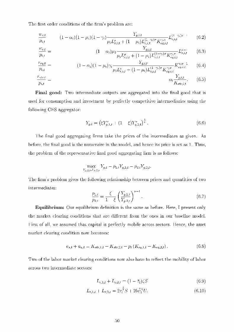
The �rst order conditions of the �rm's problem are:

wc;t

pi;t= (1� �i)(1� �i)(1� i)

Yg;i;t

�iL�r;i;t + (1� �i)L

(1� i)�c;i;t K

i�eq;i;t

L(1� i)��1c;i;t (6.2)

wr;t

pi;t= (1� �i)�2

Yg;i;t

�iL�r;i;t + (1� �i)L

(1� i)�c;i;t K

i�eq;i;t

L��1r;i;t (6.3)

req;t

pi;t= (1� �i)(1� �i) i

Yg;i;t

�iL�r;i;t + (1� �i)L

(1� i)�c;i;t K

i�eq;i;t

K i��1eq;i;t (6.4)

rstr;t

pi;t= �i

Yg;i;t

Kstr;i;t: (6.5)

Final good: Two intermediate outputs are aggregated into the �nal good that is

used for consumption and investment by perfectly competitive intermediaries using the

following CES aggregator:

Yg;t =��Y �

g;1;t + (1� �)Y �g;2;t

� 1� : (6.6)

The �nal good aggregating �rms take the prices of the intermediates as given. As

before, the �nal good is the numeraire in the model, and hence its price is set as 1. Thus,

the problem of the representative �nal good aggregating �rm is as follows:

maxYg;1;t;Yg;2;t

Yg;t � p1;tYg;1;t � p2;tYg;2;t:

The �rm's problem gives the following relationship between prices and quantities of two

intermediates:p1;t

p2;t=

�

1� �

�Yg;1;t

Yg;2;t

���1: (6.7)

Equilibrium: Our equilibrium de�nition is the same as before. Here, I present only

the market clearing conditions that are di�erent from the ones in our baseline model.

First of all, we assumed that capital is perfectly mobile across sectors. Hence, the asset

market clearing condition now becomes:

as;t + au;t = Kstr;1;t +Kstr;2;t + pt (Keq;1;t +Keq;2;t) : (6.8)

Two of the labor market clearing conditions now also have to re ect the mobility of labor

across two intermediate sectors:

Lc;1;t + Lc;2;t = (1� ��t)�S (6.9)

Lr;1;t + Lr;2;t = 2��12t S + 2b �

12t U: (6.10)

50

6.4.2 Parameterization of the three-sectors model

I keep the parameters of the baseline model the same for the extended version. Those

parameter values can be found in the �rst block of Table B.2. Keeping the baseline

parameters intact leaves eight parameters speci�c to the three-sectors version to calibrate.

Six of those are sector speci�c parameters governing the compensation shares of factors:

�1; �2; �1; �2; 1 and 2. The other two parameters come from the CES aggregator in

equation 6.6: 11��

is the elasticity of substitution between two intermediates, and � shapes

the shares of the intermediate sectors in aggregation. The calibration of each parameter

is described below in detail, and the second block of Table B.2 reports the calibrated

values.

First of all, two sectors chosen for parameterization are goods sectors including man-

ufacturing and service sectors, excluding personal services. The goods sector (sector

1) experienced, on average, 0:6 percent annual decline in the labor share, while in the

service sector (sector 2), the labor share has risen 0:12 percent each year for the years

between 1977 and 2007.6364 To obtain �1 and �2, I use the capital and output �les of

EU-KLEMS for the years between 1977 and 2007 and divide the compensation of the

non-residential structural capital by the value-added. Then I take the average as the

compensation share of the structural capital in that sector., which gives �1 = 0:1355 and

�2 = 0:0921. Similarly, to derive 1 and 2, I take the equipment capital compensation

shares from EU-KLEMS capital �le and calculate the weight of the income of the labor

associated with cognitive tasks in aggregate labor share from the CPS data. Multiplying

this weight by the labor share in the EU-KLEMS �le gives me the cognitive labor share.

Then, is are found by dividing the equipment capital compensation share by the total of

the compensation shares of equipment capital and labor employed in cognitive task occu-

pations. The obtained parameters are 1 = 0:5043 for the goods sector and 2 = 0:2653

for the service sectors. In other words, equipment capital has a substantially larger share

in production relative to cognitive tasks in the goods sector.

Similar to the parameters of the consumption aggregator, I use a simple regression

for parameterizing the �nal good aggregator in equation 6.6 as well. To begin, I take the

63If we exclude public services such as education and health, then service sector exhibits a small trend

decline as well.64The choice of period for parameterizing the sectors is constrained by the availability of detailed

capital compensation data by sectors in EU-KLEMS �les.

51

Table 6.3: Targets and Other Selected Moments for 1966

Targeted Not Targeted

Data Model Data Model

wbrcr;sec1 0:29 0:29 LSagg 0:70 0:75

wbrcr;sec1 1:02 1:02 LSsec1 0:70

LSsec2 0:77

tpcr 1:46 1:62

tpmr 0:70 0:70

wbrmr 0:11 0:06

Keq

Kstr0:78 0:66

logarithm of both sides of equation 6.7, which yields:

lnp1;t

p2;t= ln

�

1� �+ (� � 1) ln

�Yg;1;t

Yg;2;t

�:

Using NIPA tables 1.5.5 for quantity and 1.6.4 for prices for the 1967{2013 period, the

estimated regression is:

lnp1;t

p2;t= �:5204601� 1:161871 ln

�Yg;1;t

Yg;2;t

�:

This regression gives us: � = 0:3728 and � = �0:1619. This level of � implies comple-

mentarity between goods and services.

Finally, there are two weight parameters to be calibrated: �1 and �2, which are

the share of routine-task-associated occupations in the outer CES production function.

These parameters only a�ect the level of the wage-bill ratio and have no role in changes

of the labor share. As in the baseline model, I assume that the year 1966 was the initial

steady state and choose �1 and �2 to match the wage-bill ratios of each sector in 1966.

The targeted and non-targeted starting points are reported in Table 6.3. The calibrated

parameters are �1 = 0:4039 and �2 = 0:3276.

6.4.3 Solution of the extended model

The extended model is solved under perfect foresight in the same way the baseline model

is solved. As before, agents know the future paths of the relative equipment capital price

and the total factor productivity. The year 1966 is taken as the initial steady state, and

capital prices are assumed to stay at their 2013 level after this year. Later, the economy

52

is assumed to reach to a terminal equilibrium point in T years. Using the value of assets

at the initial year and consumptions T + 47 years later, I simultaneously solve the paths

of every variable between two steady states.

Two sectors face the same price and total factor productivity shocks. Furthermore,

since both labor and capital are perfectly mobile across sectors, the relative task and

capital prices are the same for each sector as well. Sectors only di�er in their initial

levels of the wage-bill ratios and the parameters governing the compensation shares of

factors. As discussed before, the parameter i, which is the share of equipment capital

in the partial Cobb-Douglas between equipment capital and cognitive tasks, is the key

parameter a�ecting the changes in the wage-bill ratio and the labor share.

Figure 6.5: Extended Model's Solution under Perfect Foresight

Series are HP-trends.

Panel (a) of Figure 6.5 shows equipment capital stock per e�cient hour at the aggre-

gate and sectoral levels. The large increases in this variable are comparable to the rise

observed in the data.65 Since equipment capital per e�cient hour rises faster in the goods

sector and there is capital-task complementarity, the wage-bill ratio between cognitive

and routine tasks also increases signi�cantly more in this sector, as shown in panel (b).

This rise in the wage-bill ratio is translated into around 20 percent decline in the labor

share of this sector, as depicted in panel (c) of Figure 6.5. On the other hand, both the

rise in the wage-bill ratio and the fall in the labor share remains limited in the service

sector.

Even though equipment capital per e�cient hour and the labor share series generated

by the model are in line with the data, the model signi�cantly overshoots the rise in the

65For instance, equipment capital per e�cient hour at the aggregate level has risen 26 times in the

data and 28 times in the model.

53

wage-bill ratio of the goods sector. To be more speci�c, the rise in the wage-bill ratio in

goods sector is 300 percent in the model, whereas it is only around 150 percent in the data.

However, model's overshooting of the wage-bill ratio does not invalidate our explanation

for the decline in the labor share through the changes in the task composition of the

wage bills. Despite quantitatively overshooting the wage-bill ratios, model qualitatively

captures two facts derived from data: (i) the larger the share of equipment capital in the

Cobb-Douglas speci�cation, the larger the rise in the wage-bill ratio and, (ii) the larger

the rise in the wage-bill ratio, the larger the fall in the labor share. These facts were

presented earlier in Figures 4.5 and 3.4, respectively.

To summarize, model is quite successful in capturing the cross-sectional di�erences

in the labor share in response to advances in technology. At this point, one can wonder

whether this is the result of di�erences in initial employment of labor devoted to routine

task occupations or weights of equipment capital in the Cobb-Douglas speci�cation. To

answer this question, I set the initial wage-bill ratios close to each other by setting �1 = �2.

The resulting transition paths of the wage-bill ratios and labor shares were similar to those

in Figure 6.5. A reverse exercise setting 1 = 2, on the other hand, eliminates sectoral

di�erences generated by the model. Thus, sectoral di�erences in terms of the labor share

trends are solely driven by the sensitivities of cost function to equipment capital prices.

7 Conclusion

This paper assesses the relationship between technological progress and the decline of

the aggregate and sectoral labor shares in the U.S. over the last few decades through the

lenses of capital-task complementarity and job polarization. With this goal in mind, an

aggregate production function for the U.S. economy|which treats three types of labor,

classi�ed by the particular tasks associated with their occupations, as di�erent inputs|

is estimated. The estimation analysis reveals that it is not labor per se that is being

substituted away. Rather, the substitution is solely away from routine tasks to both

equipment capital and non-routine tasks, and the income losses of this group account for

the entire decline of the labor share during the 1967{2013 period. When the estimated

production function is nested into a general equilibrium model, in which the where rest

of the model parameters are calibrated to the U.S. data, it shows that the decline in

equipment capital prices alone can reproduce around three-fourths of the decline in the

labor share between 1967 and 2013. The model also successfully captures heterogeneous

54

labor share trends observed across sectors.

The key insight of this paper is that changes in the occupational composition of

the labor force have played a key role in shaping the response of the labor share to

technological progress. This implies that the decline of the labor share can be considered

a natural outcome of a transition process of the U.S. economy to a new steady state with

a very low level employment share of routine task labor. Both the estimation analysis

and the dynamic general equilibrium model predict that the decline of the labor share

should come to a halt in the long run and reach a lower bound, even if equipment-speci�c

technological progress continues at its current pace. Furthermore, it also implies that

policies to train routine task labor to acquire skills compatible with non-routine cognitive

tasks would be more e�ective than tax policies in alleviating the social and economic

damages of inequalities.

References

Acemoglu, D. and D. Autor (2011). Skills, Tasks and Technologies: Implications for

Employment and Earnings, Volume 4 of Handbook of Labor Economics, Chapter 12,

pp. 1043{1171. Elsevier.

Acemoglu, D. and D. Autor (2012, June). What Does Human Capital Do? A Review of

Goldin and Katz's The Race between Education and Technology. Journal of Economic

Literature 50 (2), 426{63.

Albanesi, S., V. Gregory, C. Patterson, and A. Sahin (2013). Is job polarization holding

back the labor market? http://libertystreeteconomics.newyorkfed.org/2013/

03/is-job-polarization-holding-back-the-labor-market.html#.VeZX3kL1Jp8.

Alvarez-Cuadrado, F., N. Long, and M. Poschke (2015). Capital-labor substitution,

structural change and the labor income share. IZA Discussion Papers 8941, Institute

for the Study of Labor (IZA).

Armenter, R. (2015). A bit of a miracle no more: the decline of the labor share. Business

Review (Q3), 1{9.

Autor, D., D. Dorn, L. F. Katz, C. Patterson, and J. V. Reenen (2017, January). Con-

centrating on the fall of the labor share. Working Paper 23108, National Bureau of

Economic Research.

55

Autor, D. H. (2015). Why Are There Still So Many Jobs? The History and Future of

Workplace Automation. Journal of Economic Perspectives .

Autor, D. H. and D. Dorn (2013, August). The Growth of Low-Skill Service Jobs and the

Polarization of the US Labor Market. American Economic Review 103 (5), 1553{97.

Autor, D. H., F. Levy, and R. J. Murnane (2003, November). The Skill Content Of

Recent Technological Change: An Empirical Exploration. The Quarterly Journal of

Economics 118 (4), 1279{1333.

Beaudry, P., D. A. Green, and B. M. Sand (2013, March). The Great Reversal in the

Demand for Skill and Cognitive Tasks. NBER Working Papers 18901, National Bureau

of Economic Research, Inc.

Bisello, M. (2013, March). Job polarization in Britain from a task-based perspec-

tive.Evidence from the UK Skills Surveys. Discussion Papers 2013/160, Dipartimento

di Economia e Management (DEM), University of Pisa, Pisa, Italy.

B�ockerman, P. and M. Maliranta (2011). Globalization, creative destruction, and labour

share change: evidence on the determinants and mechanisms from longitudinal plant-

level data. Oxford Economic Papers 64 (2), 259.

Bridgman, B. (2014, October). Is Labor's Loss Capital's Gain? Gross versus Net Labor

Shares. BEA Working Papers 0114, Bureau of Economic Analysis.

Chirinko, R. S. (2008, June). [sigma]: The long and short of it. Journal of Macroeco-

nomics 30 (2), 671{686.

DiCecio, R. (2009, March). Sticky wages and sectoral labor comovement. Journal of

Economic Dynamics and Control 33 (3), 538{553.

Domeij, D. and L. Ljungqvist (2006, November). Wage Structure and Public Sector

Employment: Sweden versus the United States 1970-2002. CEPR Discussion Papers

5921, C.E.P.R. Discussion Papers.

Dustmann, C., J. Ludsteck, and U. Schnberg (2009, May). Revisiting the German Wage

Structure. The Quarterly Journal of Economics 124 (2), 843{881.

Eden, M. and P. Gaggl (2015, November). On the welfare implications of automation.

Policy Research Working Paper Series 7487, The World Bank.

56

Elsby, M., B. Hobijn, and A. Sahin (2013). The Decline of the U.S. Labor Share. Brookings

Papers on Economic Activity 47 (2 (Fall)), 1{63.

Fernandez-Macias, E. (2012). Job polarization in europe? changes in the employment

structure and job quality, 1995-2007. Work and Occupations 39 (2), 157{182.

Firpo, S., N. M. Fortin, and T. Lemieux (2011, February). Occupational Tasks and

Changes in the Wage Structure. IZA Discussion Papers 5542, Institute for the Study

of Labor (IZA).

Flood, S., M. King, S. Ruggles, and J. R. Warren (2015). Integrated Public Use Microdata

Series, Current Population Survey: Version 4.0. [machine-readable database]. https:

//cps.ipums.org/cps/.

Foote, C. L. and R. W. Ryan (2014, December). Labor market polarization over the

business cycle. Working Papers 14-16, Federal Reserve Bank of Boston.

Goos, M. and A. Manning (2007, February). Lousy and Lovely Jobs: The Rising Polar-

ization of Work in Britain. The Review of Economics and Statistics 89 (1), 118{133.

Goos, M., A. Manning, and A. Salomons (2011, December). Explaining job polarization:

the roles of technology, o�shoring and institutions. Center for Economic Studies - Dis-

cussion papers ces11.34, Katholieke Universiteit Leuven, Centrum voor Economische

Studin.

Gordon, R. J. (1990, October). The Measurement of Durable Goods Prices. Number

gord90-1 in NBER Books. National Bureau of Economic Research, Inc.

Gort, M., J. Greenwood, and P. Rupert (1999, January). Measuring the Rate of Techno-

logical Progress in Structures. Review of Economic Dynamics 2 (1), 207{230.

Greenwood, J., Z. Hercowitz, and P. Krusell (1997, June). Long-Run Implications of

Investment-Speci�c Technological Change. American Economic Review 87 (3), 342{

62.

Guerriero, M. (2012). The labour share of income around the world: Evidence from

a panel dataset. Development Economics and Public Policy Working Paper 32/12,

University of Manchester.

57

Guerriero, M. and K. Sen (2012, June). What Determines the Share of Labour in National

Income? A Cross-Country Analysis. IZA Discussion Papers 6643, Institute for the

Study of Labor (IZA).

Hansen, G. D. and L. E. Ohanian (2016, March). Neoclassical models in macroeconomics.

Working Paper 22122, National Bureau of Economic Research.

Ikenaga, T. and R. Kambayashi (2010). Long-term Trends in the Polarization of the

Japanese Labor Market: The Increase of Non-routine Task Input and Its Valuation in

the Labor Market.

Jaimovich, N. and H. E. Siu (2012, August). The Trend is the Cycle: Job Polarization

and Jobless Recoveries. NBER Working Papers 18334, National Bureau of Economic

Research, Inc.

Jorgenson, D. W. (2012, Fall). The World KLEMS Initiative. International Productivity

Monitor 24, 5{19.

Kaldor, N. (1957). A model of economic growth. The Economic Journal 67, 591{624.

Kampelmann, S. and F. Rycx (2011, January). Task-Biased Changes of Employment

and Remuneration: The Case of Occupations. IZA Discussion Papers 5470, Institute

for the Study of Labor (IZA).

Karabarbounis, L. and B. Neiman (2014a, October). Capital Depreciation and Labor

Shares Around the World: Measurement and Implications. NBER Working Papers

20606, National Bureau of Economic Research, Inc.

Karabarbounis, L. and B. Neiman (2014b). The Global Decline of the Labor Share. The

Quarterly Journal of Economics 129 (1), 61{103.

Katz, L. F. and K. M. Murphy (1992, February). Changes in Relative Wages, 1963-1987:

Supply and Demand Factors. The Quarterly Journal of Economics 107 (1), 35{78.

Koh, D., R. Santaeulalia-Llopis, and Y. Zheng (2015, April). Labor Share Decline and

the Capitalization of Intellectual Property Products.

Krusell, P., L. E. Ohanian, J.-V. Rios-Rull, and G. L. Violante (2000, September).

Capital-Skill Complementarity and Inequality: A Macroeconomic Analysis. Econo-

metrica 68 (5), 1029{1054.

58

Lawrence, R. Z. (2015, June). Recent declines in labor's share in us income: A preliminary

neoclassical account. Working Paper 21296, National Bureau of Economic Research.

Leon-Ledesma, M. A., P. McAdam, and A. Willman (2010, September). Identifying

the Elasticity of Substitution with Biased Technical Change. American Economic

Review 100 (4), 1330{57.

Leon-Ledesma, M. A., P. McAdam, and A. Willman (2015, 02). Production Technology

Estimates and Balanced Growth. Oxford Bulletin of Economics and Statistics 77 (1),

40{65.

Nellas, V. and E. Olivieri (2012). Job Polarization and Labor Market Institution.

Ober�eld, E. and D. Raval (2014, September). Micro Data and Macro Technology. NBER

Working Papers 20452, National Bureau of Economic Research, Inc.

Ohanian, L. E. and M. Orak (2016). Capital-Skill Complementarity, Inequality, and

Labor's Share of Income, 1963-2013.

O'Mahony, M. and M. P. Timmer (2009, 06). Output, Input and Productivity Measures

at the Industry Level: The EU KLEMS Database. Economic Journal 119 (538), F374{

F403.

Orak, M. (2013). From Job Polarization to Wealth Inequality: A Quantitative Test of

Routinization Hypothesis.

Orak, M. (2015, May). Is Information Technology Hurting Labor?

Piketty, T. (2014, April). Capital in the Twenty-First Century. Handbook of Labor

Economics. Belknap Press.

Piketty, T. and G. Zucman (2014). Capital is Back: Wealth-Income Ratios in Rich

Countries 1700?2010. The Quarterly Journal of Economics 129 (3), 1255{1310.

Polgreen, L. and P. Silos (2005). Capital-skill complementarity and inequality: a sensi-

tivity analysis. Technical report.

Polgreen, L. and P. Silos (2008, April). Capital-Skill Complementarity and Inequality: A

Sensitivity Analysis. Review of Economic Dynamics 11 (2), 302{313.

Polgreen, L. and P. Silos (2009, April). Crude substitution: The cyclical dynamics of oil

prices and the skill premium. Journal of Monetary Economics 56 (3), 409{418.

59

Rognlie, M. (2015, March). Deciphering the fall and rise in the net capital share. Brookings

Papers on Economic Activity .

Smith, C. L. (2013). The dynamics of labor market polarization. Technical report.

Spitz-Oener, A. (2006, April). Technical Change, Job Tasks, and Rising Educational

Demands: Looking outside the Wage Structure. Journal of Labor Economics 24 (2),

235{270.

60

APPENDIX

A Additional Figures

Figure A.1: Growth of Relative Price and Stock of Equipment Capital

Both the price and stock data are relative to structural capital.

Source: Author's calculations from the data set of DiCecio (2009) and NIPA tables.

Figure A.2: Income Share of Non-Routine Labor relative to Capital Share

Source: Author's calculations from NIPA and CPS.

61

Figure A.3: Labor Share Trend Coe�cients, by Sectors and Tasks

The y-axis shows the coe�cient of the regression of log of the labor share on a constant and a

time variable. In this sense, this coe�cient shows the annual growth rate of the labor share.

Due to the small number of data for manual labor for many sectors, cognitive and manual labor

are aggregated as non-routine labor.

Source: Author's calculations from labor and output �les of the WORLD-KLEMS and CPS

data sets.

62

Figure A.4: Model Fit and Data for the Cobb-Douglas Speci�cation

The series are HP-trends.

The model plots are derived from the estimation of the model with the Cobb-Douglas speci�-

cation as in equation 4.14

63

Figure A.5: E�ect of the Changes in Wage-Bill Ratio on Labor Share Growth

The �gure shows the coe�cient of the changes in wage-bill ratio in equation 4.17.

Figure A.6: Labor Share Generated by the Wage-Bill Ratio Series for Selected Sectors

The series are HP-trends.

The �gure shows the model �t when equation 4.17 is fed with the wage-bill ratios and s

calibrated for each sector.

64

B Additional Tables

Table B.1: Abbreviations of the Sectors

Abbreviation Sector

AGRI Agriculture, Hunting and Fishery

BUSN Real Estate and Business

CHEM Chemicals and Chemical Products

COMM Post and Telecommunication

CONS Construction

EDUC Educational Services

ELEQ Electrical and Optical Equipment

FINI Financial Intermediation

FOOD Food, Tobacco and Beverage

FURN Furniture and Recycling

HEAL Health Services

HOTR Hotels and Restaurants

MACH Machinery Equipment

META Basic and Fabricated Metal

MINE Non-Metallic Products

MING Mining and Quarrying

MVCT Motor Vehicles Trade

PERS Other Personal Services

PETR Coke and Re�ned Petroleum

PULP Pulp, Paper and Printing

RETT Retail Trade and Repair

RUBB Rubber and Plastic Products

TEXT Textile, Leather and Footwear

TRAN Transportation and Storage

TREQ Transport Equipment

UTIL Utilities

WHST Wholesale Trade and Commission

WOOD Wood and Cork Products

65

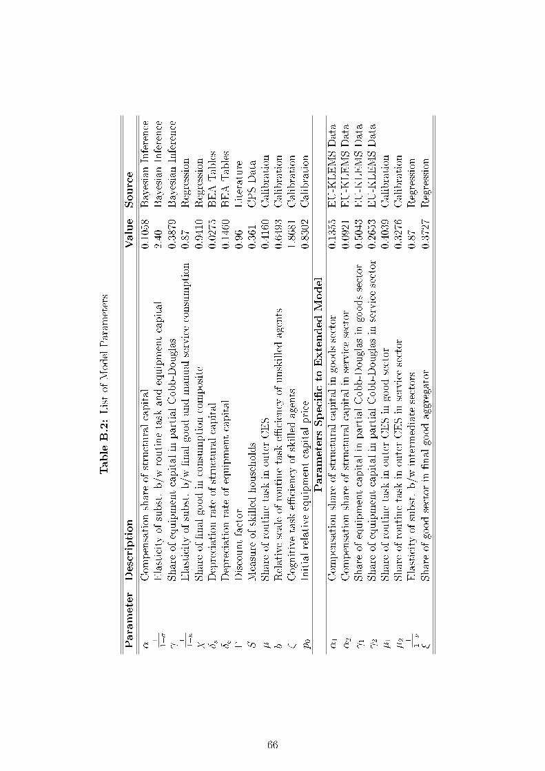
TableB.2:ListofModelParam

eters

Parameter

Description

Value

Source

�Com

pensation

shareofstructuralcapital

0:1058

BayesianInference

11��

Elasticityofsubst.b/w

routinetask

andequipmentcapital

2:40

BayesianInference

Shareofequipmentcapitalin

partialCobb-Douglas

0:3879

BayesianInference

11��

Elasticityofsubst.b/w

�nalgoodandmanualserviceconsumption

0:87

Regression

�Shareof�nalgoodin

consumption

composite

0:9410

Regression

� sDepreciationrate

ofstructuralcapital

0:0275

BEATables

� eDepreciationrate

ofequipmentcapital

0:1460

BEATables

�Discountfactor

0:96

Literature

SMeasure

ofskilledhouseholds

0:361

CPSData

�Shareofroutinetask

inouterCES

0:4160

Calibration

bRelativescaleofroutinetask

e�ciency

ofunskilledagents

0:6493

Calibration

�Cognitivetask

e�ciency

ofskilledagents

1:8681

Calibration

p0

Initialrelative

equipmentcapitalprice

0:8302

Calibration

ParametersSpeci�cto

ExtendedModel

�1

Com

pensation

shareofstructuralcapitalin

goodssector

0:1355

EU-KLEMSData

�2

Com

pensation

shareofstructuralcapitalin

servicesector

0:0921

EU-KLEMSData

1

Shareofequipmentcapitalin

partialCobb-Douglas

ingoodssector

0:5043

EU-KLEMSData

2

Shareofequipmentcapitalin

partialCobb-Douglas

inservicesector

0:2653

EU-KLEMSData

�1

Shareofroutinetask

inouterCESin

goodsector

0:4039

Calibration

�2

Shareofroutinetask

inouterCESin

servicesector

0:3276

Calibration

11��

Elasticityofsubst.b/w

interm

ediate

sectors

0:87

Regression

�Shareofgoodsector

in�nalgoodaggregator

0:3727

Regression

66

C Derivations and Equations

C.1 Representative Firm's First Order Conditions

The �rst order conditions below are with respect to cognitive, routine, and manual tasks

and structural and equipment capitals in this speci�c order.

C.1.1 General functional form

wc = (1� �)(1� �)�(1� �)Y�

�L�r + (1� �)�� [�K�

eq + (1� �)L�c ]�� + (1� �)L�m

���

�

�

����K�

eq + (1� �)L�c��� + (1� �)L�m

����1 �

�K�eq + (1� �)L�c

����1 L

�c

hc(C.1)

wr = (1� �)�Y�

�L�r + (1� �)�� [�K�

eq + (1� �)L�c ]�� + (1� �)L�m

���

� L�rhr

(C.2)

wm = (1� �)(1� �)(1� �)Y�

�L�r + (1� �)�� [�K�

eq + (1� �)L�c ]�� + (1� �)L�m

���

�

�

����K�

eq + (1� �)L�c��� + (1� �)L�m

����1

L�m

hm(C.3)

rstr = �Y

Kstr(C.4)

req = (1� �)(1� �)��Y�

�L�r + (1� �)�� [�K�

eq + (1� �)L�c ]�� + (1� �)L�m

���

�

�

����K�

eq + (1� �)L�c��� + (1� �)L�m

����1 �

�K�eq + (1� �)L�c

����1

K��1eq (C.5)

C.1.2 Cobb-Douglas speci�cation

wc = (1 � �)(1 � �)�Y�

�L�r + (1� �)hL�cK

eqL

1� ��m

i��K� eq L

�(1��� )m

L��chc

(C.6)

wr = (1� �)�Y�

�L�r + (1� �)hL�cK

eqL

1� ��m

i�� L�r

hr(C.7)

wm = (1 � �)(1 � �)(1 � � � )Y�

�L�r + (1� �)hL�cK

eqL

1� ��m

i��K� eq L

��c

L�(1��� )m

hm(C.8)

rstr = �Y

Kstr(C.9)

67

req = (1 � �)(1 � �) Y�

�L�r + (1� �)hL�cK

eqL

1� ��m

i��K� �1eq L�(1��� )m L��c (C.10)

C.2 Relationship between Labor Share and Wage-Bill Ratio

LSt =wr;thr;t + wc;thc;t + wm;thm;t

Yt(C.11)

LSt = (1� �)�L�r;t + (1� �)�K�

eq;tL��c;tL

�(1��� )m;t + (1� �)(1� � �)K�

eq;tL��c;tL

�(1��� )m;t�

�L�r;t + (1� �)hK eq;tL

�c;tL

1��� m;t

i��(C.12)

LSt = (1� �)�L�r;t + (1� �)(1� )K�

eq;tL��c;tL

�(1��� )m;t�

�L�r;t + (1� �)hK eq;tL

�c;tL

1��� m;t

i�� (C.13)

Multiplying both denominator and numerator of the right hand side by 1�L�r;t

LSt = (1� �)1 +

(1��)(1� )K� eq;tL

��c;tL

�(1��� )m;t

�L�r;t

1 +(1��)K�

eq;tL��c;tL

�(1��� )m;t

�L�r;t

(C.14)

Multiplying the second term in the denominator by 1� 1�

:

LSt = (1� �)1 +

(1��)(1� )K� eq;tL

��c;tL

�(1��� )m;t

�L�r;t

1 +(1��)K�

eq;tL��c;tL

�(1��� )m;t

�L�r;t

1� 1�

(C.15)

LSt = (1� �)1 +

(1��)(1� )K� eq;tL

��c;tL

�(1��� )m;t

�L�r;t

1 +

(1��)(1� )K� eq;tL

��c;tL

�(1��� )m;t

�L�r;t

1�

(C.16)

Substituting the wage-bill ratio between non-routine and routine tasks:

wbrt =(1� �)(1� )K�

eq;tL��c;tL

�(1� ��)m;t

�L�r;t(C.17)

LSt = (1� �)1 + wbrt

1 + wbrt1�

(C.18)

C.3 Labor Share in Di�erence Terms

Below, the variables with a hat denote growth rate of the variable from period t� 1 to t.

Equation C.18 can be written in growth terms as follows:

cLSt = \(1 + wbrt)�\

�1 +

wbrt

1�

�(C.19)

68

cLSt = wbrt

1 + wbrtdwbrt � wbrt

1�

1 + wbrt1�

dwbrt (C.20)

cLSt = wbrt

1 + wbrtdwbrt � wbrt

1� + wbrtdwbrt (C.21)

cLSt = (1� )wbrt + wbr2t(1� ) + wbrt + (1� )wbrt + wbr2t

dwbrt� wbrt + wbr2t(1� ) + wbrt + (1� )wbrt + wbr2t

dwbrt(C.22)cLSt = dwbrt � wbrt � wbrt + wbr2t � wbrt � wbr2t

(1� ) + wbrt + (1� )wbrt + wbr2t

�(C.23)

cLSt = �dwbrt � wbrt

(1� ) + (2� )wbrt + wbr2t

�(C.24)

cLSt = �dwbrt "

wbrt + (2� ) + (1� )wbrt

#(C.25)

D Labor Input and Wage Data

D.1 Measuring Labor Input and Wage Rates

This methodology closely follow from Krusell et al. (2000) and Domeij and Ljungqvist

(2006). Labor data is obtained from March Current Population Survey (CPS) integrated

by IPUMS (Flood et al. (2015)). The availability of a consistent occupational de�ni-

tion limits the period of study to 1967 to 2013. Number of annual observations in raw

data ranges from 130,476 (1996) to 218,269 (2001). However, after dropping out some

observations, we are left with numbers ranging from 55,721 (1996) to 96,184 (2001). I

record every person whose age is between 16 and 70. Consistent with the literature,

self-employed people, unpaid family workers and agricultural and military workers are

dropped from the sample. Furthermore, people who reported zero usual hours worked

per week last year are dropped as well.

For each person, I record their personal characteristics: age, sex, race, occupation

(occ50ly); employment statistics: class of worker (classwly), weeks worked last year

(wkswork1 and wkswork2 ), usual hours worked per week last year (uhrswork and hr-

swork1 ); income: total wage and salary income last year (incwage) and CPS personal

supplement weights: wtsupp.66 Three task groups are obtained from the occupation se-

ries based on the classi�cations in the literature. The details of this can be found in the

following subsection. Then, each person is assigned to one of 198 groups created by age,

race, sex and task. Age is divided into 11 �ve-year groups: 16-20, 21-25, 26-30, 31-35,

66IPUMS recodes the CPS series on occupation into the 1950 Census Bureau occupational classi�cationsystem. This provides consistent occupational codes for the jobs respondents reported working duringthe previous calendar year, for 1968 forward.

69

36-40, 41-45, 46-50, 51-55, 56-60, 61-65, 66-70. Race is divided into three: white, black,

others. Finally, occupation is divided into three task groups: cognitive, routine, and

manual.

Before calculating the annual hours worked and hourly wage rates, top-coded income

values are adjusted using the \revised income top-codes �les" published by Census Bureau

(and compiled by IPUMS) to swap top-coded values in 1976{2010 CPS �les with these

revised values. This procedure replaces the top-coded values with new values based on

the Income Component Rank Proximity Swap method, which was introduced in 2011.

Hence, throughout the whole 1975{2013 period, the top-coding methodology is consistent

and comparable. This also eliminates the jumps in task premium that researchers observe

due to the change in topcoding methodology in some years. Unfortunately, swap values

are not available for earlier years. Therefore, following Krusell et al. (2000), I tried both

leaving the top-coded values as they are and also multiplying them by 1.45 for the years

before 1975. Switching from one practice to the other does not change any of the results

of the paper.

For the CPS years after 1975, CPS has usual hours worked per week and weeks worked

last year. Thus, calculating the annual hours for a person is straightforward: I simply

multiply weeks worked last year by usual hours worked. Hence, for CPS years 1976 and

afterwards, total hours are:

hoursi;t�1 = wkswork1i;t�1 � uhrsworki;t�1;

where, i is individual observation and t is the CPS year.

For earlier years, I need to do two adjustments. First, weeks worked are available

only as intervals and I need to approximate a scalar value for each interval. Fortunately,

both the intervals and actual weeks are available for years after 1975. Therefore, we

can calculate the average weeks worked after year 1975 for each interval and replace the

earlier years with those values. In this context, the following approximations are used:

70

Interval Approximation

1-13 8.1

14-26 21.5

27-39 33.6

40-47 42.6

48-49 48.3

50-52 51.8

Second, I have to use hours worked last week variable as a proxy to usual hours

worked per week last year. However, there are many agents who were not employed last

week or who were employed but not at work for some reason, despite reporting a positive

income for last year. Rather than dropping those observations, I replaced the hours they

worked per week with the average of the hours worked by the people in their group in

that particular year. I also paid attention to whether the person was employed part time

or full time when doing this replacement.

Hourly wage is calculated as:

wagei;t�1 =incwage swappedi;t�1

hoursi;t�1:

Later, observations with hoursi;t�1 < 260 (quarter of part time work) and wagei;t�1 <

0:5 �minimum waget�1 are dropped to smooth out the e�ect of externalities and mis-

reporting. Following this, for each groups and year, I calculate group weights as: �g;t =Pi2g �i;t where, g 2 G is set of groups. Then average hours and wage measures for each

group and year are calculated:

hoursg;t�1 =

Pi2g �i;t � hoursi;t�1

�g;t

wageg;t�1 =

Pi2g �i;t � wagei;t�1

�g;t:

To aggregate across groups into aggregate task groups, the group wages of 1980 are

used as the weights. Letting j 2 fC;R;Mg, where C, R and M represent the cognitive,

routine and manual occupations respectively, then for each task group j, we have total

hours:

Nj;t�1 =Xg2Gj

hoursg;t�1 � �g;t � wageg;80;

71

and average hourly wage is:

Wj;t�1 =

Pg2Gj

hoursg;t�1 � �g;t � wageg;t�1

Nj;t�1:

Finally task premium between cognitive and routine tasks is calculated asWC;t�1

WR;t�1:.

The other task premiums are found in the same way.

D.2 Occupational Classi�cation

I follow Autor et al. (2003), Acemoglu and Autor (2011), Jaimovich and Siu (2012)

Autor and Dorn (2013)|among many other studies in the literature|to classify the

occupations into di�erent tasks. Occupations are divided along two dimensions: cognitive

versus manual and routine versus non-routine. Table D.1 provides detailed explanations

and examples for each of these categories.67 In short, cognitive and manual jobs are

characterized by the di�erences in the extent of mental versus physical activity. On

the other hand, routine and non-routine jobs are di�erentiated based on how easily the

work can be codi�ed. Routine tasks are the ones that can be summarized as a set of

speci�c activities accomplished by following well-de�ned instructions and procedures.

In contrast, when a task requires instant decision making, exibility, taking initiatives,

problem solving, creativity, and personal interaction, then it is classi�ed as non-routine.

Table D.1: Occupational Classi�cation

Non-Routine Routine

Cognitive Managerial, professional, technicalworkers (namely, physicians, pub-lic relations managers, �nancialanalysts, computer programmers,economists)

Sales and o�ce and administrativesupport (namely, secretaries, banktellers, retail salespeople, travelagents, mail clerks, data entry key-ers)

Manual Service jobs (namely, janitors, gar-deners, manicurists, bartenders,home health asides)

Blue collar jobs (namely, machineoperators and tenders, mechanics,dress makers, fabricators and as-semblers, cement masons, and meatprocessing workers)

For the purpose of this study|and as common in the literature|I classify all the

routine occupations in one single category: \Routine", whether they are cognitive or

manual. This group represents the tasks implemented by the \middle-skill" labor. These

67This section and table are mostly borrowed from the work of Jaimovich and Siu (2012).

72

occupations are not necessarily mechanical nor computerized and they might even require

personal interaction. The common characteristic of the tasks labeled as routine is that

they can be replaced by technological improvement or can be o�shored. For instance, as

online sales became more widespread, many sale jobs have been lost. As another example,

most of the call centers started employing labor that is physically in India.

Non-routine occupations are divided into two categories. I label cognitive non-routine

occupations as \Abstract", which tends to be \high-skill" labor. These are mainly man-

agerial, professional, executive, and technical jobs. Finally, manual non-routine occupa-

tions are classi�ed as \Manual" occupations. These occupations represent the lowest tail

of the skill distribution and they are termed as \service occupations" by Autor and Dorn

(2013) and Firpo et al. (2011).

73