Federal Reserve Bank of Minneapolis

Research Department Staff Report 451

Revised January 2012

Capital Taxation During the U.S. Great Depression∗

Ellen R. McGrattan

Federal Reserve Bank of Minneapolis

and University of Minnesota

ABSTRACT

Previous studies of the U.S. Great Depression find that increased government spending and taxa-

tion contributed little to either the dramatic downturn or the slow recovery. These studies include

only one type of capital taxation: a business profits tax. The contribution is much greater when

the analysis includes other types of capital taxes. A general equilibrium model extended to include

taxes on dividends, property, capital stock, excess profits, and undistributed profits predicts pat-

terns of output, investment, and hours worked that are more like those in the 1930s than found

in earlier studies. The greatest effects come from the increased taxes on corporate dividends and

undistributed profits.

∗Appendices, data, and codes are available at my website, www.minneapolisfed.org/research/sr/sr451.html. For

helpful comments, I thank Roozbeh Hosseini, Ayse Imrohoroglu, Lee Ohanian, Ed Prescott, Martin Schneider,

the editor, five anonymous referees as well as conference participants at the Center for the Advanced Study in

Economic Efficiency and seminar participants at the Norges Bank, the Institute for International Economic Studies,

the Toulouse School of Economics, the Federal Reserve Bank of Minneapolis, the University of Virginia, Harvard

University, and the University of Pennsylvania. For editorial assistance, I thank Kathy Rolfe and Joan Gieseke. The

views expressed herein are those of the author and not necessarily those of the Federal Reserve Bank of Minneapolis

or the Federal Reserve System.

1

I. Introduction

Although there is no general agreement on the primary causes of the U.S. Great Depression—

defined as both the sharp economic contraction in the early 1930s and the subsequent slow

recovery—many do agree that fiscal policy played only a minor role. This conventional view

is based on both empirical and theoretical analyses of the period. Although federal government

spending notably increased during the 1930s, the data show that as a share of GDP, it did not in-

crease enough to have had a large impact on economic activity overall (Brown, 1956). At the same

time, income tax rates increased sharply, but taxes were filed by few households and paid by even

fewer (Seltzer, 1968).1 Feeding estimates of spending and tax rates into a standard neoclassical

growth model, Cole and Ohanian (1999) confirm that the impact of fiscal policy during the 1930s

was too small to matter. Here, I challenge that conventional view by extending the basic growth

model in ways suggested by actual U.S. fiscal policies in the 1930s. My extended model improves

on the basic model’s predictions of U.S. economic activity during that decade and strongly suggests

that fiscal policy did, in fact, play a major role in the Great Depression.

My primary extension is to include capital taxes that are not typically included in the basic

growth model analyzed by Cole and Ohanian (1999) and many others. Standard practice is to

model capital taxes as taxes on business profits.2 I look as well at taxes on capital stock, prop-

erty, excess profits, undistributed profits, and dividends. When these overlooked capital taxes are

incorporated into the neoclassical framework, along with taxes on normal business profits, labor,

and consumption, the model predicts patterns in aggregate economic activity that are much closer

to those in U.S. data, especially U.S. investment, than previous studies have found.

Differentiating capital taxes paid by businesses and those paid by individuals plays a key role

for my results. A major fiscal policy change in the 1930s is the sharp increase in tax rates on indi-

vidual incomes, which include corporate dividends. Although few households paid income taxes,

those who did earned almost all of the income distributed by corporations and unincorporated

businesses. If the increases in rates were not completely unexpected, these households would have

foreseen large declines in future gross returns on investments. An optimal response by compa-

nies would have been to distribute earnings in advance of the tax increases rather than to reinvest

them. Thus, increasing the tax rate on dividends has a significant effect on investment, even before

1932 when major changes were enacted. If, in addition to raising individual income tax rates, the

1 The percentage of the total population covered by taxable returns was 4.1 percent in 1929 and only 2.6 percentby 1933.

2 See, for example, the business cycle studies of Braun (1994) and McGrattan (1994) and the Great Depressionstudies in Kehoe and Prescott (2007).

2

government introduces a tax on the undistributed profits of corporations, as the U.S. government

did in 1936, then investment is again negatively impacted. The introduction of such a tax would

naturally affect the recovery in the second half of the 1930s.

With a tax system that includes key features of U.S. policy and uncertainty about future

tax rates, the extended model predicts U.S. economic activity significantly better than the basic

model. That model predicts strongly counterfactual changes between 1929 and 1932: for example,

a 1 percent rise in GDP instead of a 31 percent fall and a 2 percent rise in per capita hours

worked instead of a 27 percent fall. The extended model predicts declines in both of these series,

predictions that account for about 36 percent of the actual decline in GDP and 38 percent of the

actual decline in hours of work. Perhaps more dramatically, the extended model improves on the

predicted path of investment. Over the decade, U.S. investment first dropped sharply, between

1929 and 1932, then recovered a bit before again dropping sharply in 1938. The basic model badly

misses that pattern; the extended model captures it. The extended model also does a better job

in predicting the drop in equity values, which fell by roughly 30 percent by the end of the decade.3

A closer look at the quantitative results reveals an important difference between taxing profits

and taxing dividends. An increase in the tax rate on profits lowers the net return to capital. To

have a large impact on the gross return to capital, the tax rate on profits would have had to rise

significantly more than it did during the 1930s. On the other hand, assuming households expect a

change in policy, an increase in the tax rate on dividends lowers the gross return to capital. Thus,

changes in tax rates on dividends that are comparable in magnitude to changes in tax rates on

profits have a much larger impact on the model’s predictions, especially for investment. Variations

in household expectations do affect the timing of the declines in investment, but I find that all

settings within an empirically plausible range yield large declines in investment, like those observed

in U.S. data.

Factors other than tax policy clearly were involved in the deep downturn and slow recovery of

the 1930s. This is demonstrated, for example, by the fact that the initial consumption predictions

do not line up well with the data. U.S. consumption fell sharply in the early part of the 1930s,

yet both the basic model and the extended model miss that drop. In fact, the extended model

actually predicts an initial rise. Expectations of higher future capital tax rates imply a sharp initial

increase in distributions of business incomes, accomplished by decreasing investment. Increased

distributions then lead, counterfactually, to increased consumption, which falls only when higher

3 In McGrattan (2012), I include intangible investments in the model because they can be expensed and thuslower taxable business profits. The main quantitative results are similar.

3

sales and excise taxes are imposed. Adding New Deal policies (as in the 2004 work of Cole and

Ohanian) would help further account for the time series patterns in the later part of the decade.

But we need other ways to account for the pattern of consumption in the early part.

In related work, Bernanke and Gertler (1989) and Ohanian (2009) use versions of the neo-

classical growth model motivated by the U.S. experience in the Great Depression, especially the

large contraction early in the decade. Bernanke and Gertler (1989) introduce an asymmetry of

information between borrowers and lenders that exacerbates negative shocks to the net worth of

investors. Their theory formalizes the view that periods of financial crisis are typified by low and

inefficient investment. Ohanian (2009) introduces cartelization in the manufacturing sector and

assumes that firms keep real wages high and weekly hours low. His theory formalizes the view that

Herbert Hoover’s industrial labor program started the Great Depression. Neither Bernanke and

Gertler (1989) nor Ohanian (2009) includes a role for capital taxes.

The paper is organized as follows. In Section II, I describe extensions to the basic neoclassical

growth model that are central to the analysis. In Section III, I describe the source and construction

of the main model inputs: tax rates, spending, and policy expectations. In Section IV, I compare

the extended model’s predictions to U.S. data and to predictions of the basic model, quantifying

the role of fiscal policies and expectations. In Section V, I investigate the role of expectations

and two key capital taxes. In Section VI, I provide some cross-country evidence in support of my

findings. Section VII concludes.

II. Theory

To analyze U.S. fiscal policy in the 1930s, I use an extension of the basic neoclassical growth

model that includes a more comprehensive specification of taxes than is typically used. Specifically,

I include taxes on property, capital stock, excess profits, undistributed profits, dividends, and sales

in addition to taxes on wages and normal business profits analyzed by Cole and Ohanian (1999).

Consider first the problem solved by households. Given the initial capital stock k0, the stand-

in household chooses consumption c, investment x, and hours worked h to maximize expected

utility

E∞∑

t=0

βt{log (ct) + ψ log (1 − ht)}Nt

subject to the constraints

ct + xt = rtkt + wtht + κt − ζt,(1)

4

kt+1 = [(1 − δ) kt + xt] / (1 + η) ,(2)

and nonnegativity constraints on investments xt ≥ 0, where variables are written in per capita

terms, Nt = N0(1 + η)t is the population in t, which grows at rate η, β is the time discount factor,

ψ is a parameter governing the disutility of work, and δ is the depreciation rate of capital. Capital

is paid rent rt; labor is paid wage wt. Per capita transfers are given by κt and taxes by ζt.

The firms’ aggregate production technology is given by

(3) Yt = Kθt (ZtHt)

1−θ,

where capital letters denote aggregates and θ is the capital share of output. The parameter Zt

is labor-augmenting technical change that is assumed to grow at a constant rate, Zt = (1 + γ)t.

The firm rents capital and labor. If profits are maximized, then the rental rates are equal to the

marginal products. The goods market clears, so Nt(ct + xt + gt) = Yt, where gt is per capita

government spending.

Two versions of the model are considered and differ in the specifications of taxes and transfers.

In the basic model, taxes are the sum of taxes on labor income and profits to capital,

(4) ζt = τhtwtht + τpt (rt − δ) kt,

where τht is the tax rate on labor income and τpt is the tax rate on profits. Transfers are determined

residually as revenues less spending, κt = ζt − gt, and paid as a lump sum to households. The

transfers are taken as given by households when solving their maximization problem.

In the extended model, I include additional taxes in the formula for ζt and, because my focus

is taxation of business capital, I distinguish between business and nonbusiness activity. Let xbt

and xnt = xt − xbt denote business and nonbusiness investment, respectively. Similarly, let kbt

and knt = kt − kbt denote business and nonbusiness capital stocks. The formula for taxes in the

extended model is given by

ζt = τhtwtht + τpt (rt − δ − τkt) kbt(5)

+ τctct + τktkbt + τut ((1 + η) kb,t+1 − kbt)

+ τdt{rtkbt − xbt − τpt (rt − δ − τkt) kbt − τktkbt − τut ((1 + η) kb,t+1 − kbt)},

where τpt is now the tax rate on business profits, τct is the tax rate on consumption, τkt is the tax

rate on business property, τut is the tax rate on undistributed profits, and τdt is the tax rate on

5

dividends. Note that taxable income for the tax on profits is net of depreciation and property tax,

and taxable income for the tax on dividends is net of taxes on profits, property, and undistributed

profits.

The formula in equation (5) includes capital taxes on business activities, which are assumed to

be those of corporations and nonfarm proprietors. Tax revenues from the nonbusiness sector, which

accounts for about 36 percent of U.S. value added, are included with transfers. This is convenient

because I assume that choices of nonbusiness output, investment, and hours are set exogenously

to be consistent with U.S. time series. I do this to ensure that my model accounts line up with

the U.S. national accounts. Specifically, nonbusiness output, which I denote ynt, less nonbusiness

investment xnt and any taxes on nonbusiness incomes is (exogenously) included with transfers to

households κt. With nonbusiness net income included with transfers, equations (1)–(3) can be

rewritten with business components of capital, labor, and investment replacing the aggregates.4

GDP in both the basic and extended versions of the model is the sum of private consumption

c, public consumption g, and investment x; in per capita terms, GDP is thus c+ g + x. The value

of business capital is given by

(6) Vt = (1 − τdt) (1 + τut)Kbt+1,

where Kbt+1 is the aggregate end-of-year business capital stock. Notice that the value is directly

affected by capital taxes through prices of capital and indirectly affected by capital taxes through

their effects on the time variation of capital.

The formulation for ζt in equation (5) assumes that businesses finance investment with internal

funds rather than with external funds. This choice is motivated by data on sources of funds of

nonfinancial corporations from Goldsmith (1958, Table 53). Goldsmith’s series shows that 98

percent of investment funds of nonfinancial corporations were supplied by internal sources over

the period 1934–1939 when business investment was rising. An important factor determining the

financing decision is the cost of security flotation. Surveys done by the Securities and Exchange

Commission (1941, Table 1) show high costs of flotation for issues of common stock. For example,

in 1938, a sample of 81 firms issuing stock through investment bank facilities had average costs of

20.1 percent of the amount issued. Costs for bond issues were lower, but Goldsmith’s data show

that borrowing was not an important source of funds during the 1930s. In a study of firm-level

data in 1936, Calomiris and Hubbard (1995) find that only one in four firms issued bonds, with 10

4 See the time paths of U.S. nonbusiness activity in the Appendix, Table A.1. These series are treated as inputsfor the extended model simulations.

6

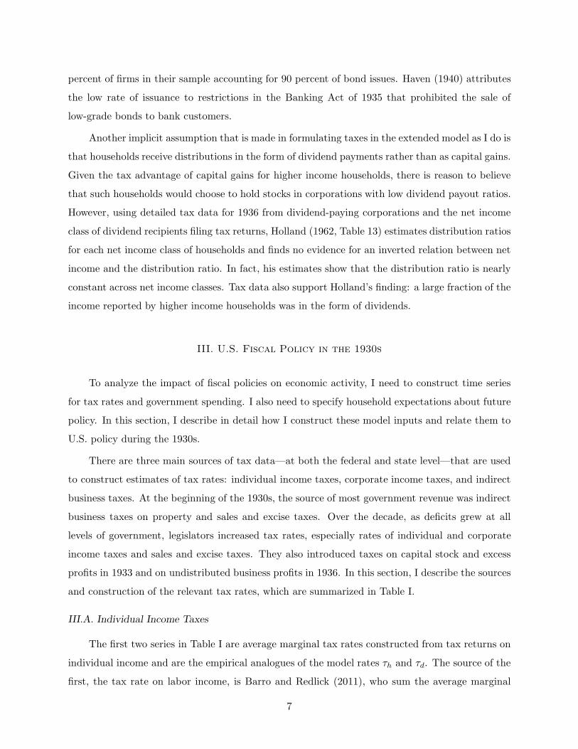
percent of firms in their sample accounting for 90 percent of bond issues. Haven (1940) attributes

the low rate of issuance to restrictions in the Banking Act of 1935 that prohibited the sale of

low-grade bonds to bank customers.

Another implicit assumption that is made in formulating taxes in the extended model as I do is

that households receive distributions in the form of dividend payments rather than as capital gains.

Given the tax advantage of capital gains for higher income households, there is reason to believe

that such households would choose to hold stocks in corporations with low dividend payout ratios.

However, using detailed tax data for 1936 from dividend-paying corporations and the net income

class of dividend recipients filing tax returns, Holland (1962, Table 13) estimates distribution ratios

for each net income class of households and finds no evidence for an inverted relation between net

income and the distribution ratio. In fact, his estimates show that the distribution ratio is nearly

constant across net income classes. Tax data also support Holland’s finding: a large fraction of the

income reported by higher income households was in the form of dividends.

III. U.S. Fiscal Policy in the 1930s

To analyze the impact of fiscal policies on economic activity, I need to construct time series

for tax rates and government spending. I also need to specify household expectations about future

policy. In this section, I describe in detail how I construct these model inputs and relate them to

U.S. policy during the 1930s.

There are three main sources of tax data—at both the federal and state level—that are used

to construct estimates of tax rates: individual income taxes, corporate income taxes, and indirect

business taxes. At the beginning of the 1930s, the source of most government revenue was indirect

business taxes on property and sales and excise taxes. Over the decade, as deficits grew at all

levels of government, legislators increased tax rates, especially rates of individual and corporate

income taxes and sales and excise taxes. They also introduced taxes on capital stock and excess

profits in 1933 and on undistributed business profits in 1936. In this section, I describe the sources

and construction of the relevant tax rates, which are summarized in Table I.

III.A. Individual Income Taxes

The first two series in Table I are average marginal tax rates constructed from tax returns on

individual income and are the empirical analogues of the model rates τh and τd. The source of the

first, the tax rate on labor income, is Barro and Redlick (2011), who sum the average marginal

7

tax rates constructed from federal income tax data published in the U.S. Treasury Department’s

Statistics of Income (SOI), the Social Security payroll tax rates, and average marginal tax rates

from state income tax data. The average marginal tax rates are weighted sums of marginal tax rates

for each income class, with weights equal to the fraction of income that the income class receives.

Specifically, if income class i pays τi on an additional dollar of income earned and earns yi/∑

i yi

of the total income, then the average marginal tax rate is computed as follows: τ =∑

i τiyi/∑

i yi.

The source of Barro and Redlick’s (2011) federal income tax rate is Barro and Sahasakul

(1983), who calculate marginal tax rates for each class of net income, the measure of income

used by the U.S. Internal Revenue Service (IRS) in the 1930s. Net income is taxable income less

exemptions. In order to compute a long time series, Barro and Sahasakul weight the marginal

rates by total incomes, which is a proxy for the measure of income used by the IRS in later years,

namely, adjusted gross income. Total adjusted gross income, for filers and nonfilers (paying a

tax rate of zero), is estimated to be 79 percent of national income and product account (NIPA)

personal income during the 1930s. Estimates of the average marginal tax rate from the Social

Security payroll tax rate, which is zero before 1937, are added by Barro and Sahasakul (1986).

To these rates, Barro and Redlick (2011) add average marginal income tax rates from state

income tax data. They do this with the help of two tax calculators: TAXSIM (Feenberg and

Coutts, 1993) and IncTaxCalc (Bakija, 2009). Starting with 1979, the first year in which state

identifiers are included in the TAXSIM database, Barro and Redlick take a sample of returns and,

for each year from 1929 through 1978, scale the components of income so that the change in per

capita incomes on the returns matches the change in per capita personal income in NIPA. They

then use IncTaxCalc, which has detailed information about tax rates by state, to compute marginal

tax rates as the change in tax liabilities from an incremental change in income.

To construct average marginal tax rates on dividend income from federal tax data, I use the

same methodology as Barro and Sahasakul (1983). Specifically, I use dividend income for each net

income class as weights and dividend income from NIPA to determine the income of nonfilers.5 For

the marginal tax rates, I use only surtaxes prior to 1936 because dividend income was not subject

to the normal rate in this period. One additional adjustment is needed because some dividend

income accrues to fiduciaries, but the SOI does not categorize it the same way each year in my

sample. Dividend income of fiduciaries is included with all other dividend income between 1929

5 NIPA table 7.16 shows the relation of IRS dividends paid by corporations and NIPA dividends in personalincome. The main differences are intercorporate dividends plus net dividend income paid to foreigners. Holland(1962) and U.S. Treasury (1948) estimate that underreported amounts on tax returns are small.

8

and 1935 and later with fiduciary income. Thus, for 1936 to 1939, I increase the SOI’s reported

dividend income by an amount equal to the SOI’s fiduciary income multiplied by an estimate of

the fraction of income fiduciaries earn from dividends. My estimate of this fraction is the ratio

of dividend income reported on IRS Form 1041 (filed by all fiduciaries) to the balance income on

Form 1041, which is the total income fiduciaries have available for distribution.

To construct the tax rates on dividends, τd, I add estimates of average marginal tax rates

for state income taxes, but use a different algorithm than do Barro and Redlick (2011), in part

because of the many policy changes that potentially impact the concentration and deferral of

dividend income between 1929 and 1979, when state identifiers are first available in TAXSIM. For

the years 1929–1939, I use state tax rate schedules from the Tax Research Foundation (1930–1942),

data on the distribution of dividend income across net income classes on federal returns from the

SOI, and data on the fraction of dividends reported on federal returns by state from the SOI. In

essence, for each year and each state, I compute an average marginal tax rate for dividend income

using the tax schedule for that year and state and the distribution of dividend incomes for that year

reported on federal tax returns.6 I then construct a weighted average across states with weights

equal to the fraction of dividend income earned by residents of the states.

III.B. Corporate Income Taxes

The tax rate on profits used in the model simulations, τp, is estimated to be the sum of the tax

rate on normal business profits and the effective rate due to the capital stock tax in combination

with the excess profits tax. For the normal business profit tax, I use the statutory corporate income

tax rate. This series is shown in the fourth column of Table I. For the excess profits tax, used in

combination with the capital stock tax, I follow Brown (1949) and treat them in combination like

an effective tax on business profits. This choice is motivated by the actual U.S. tax system in the

1930s. Companies had to declare a value for their capital stock, and a tax was assessed on that

value. To avoid having companies declare a capital value that was too low, the government used

an excess profits tax as a penalty. For example, in 1934, if profits exceeded 12.5 percent of the

declared capital stock value, then companies paid a 5 percent tax on the excess profits. To avoid

this penalty, companies tended to declare a high value for capital, and they paid roughly 2 percent

of profits because of this tax in addition to their normal tax bill. (See Brown, 1949.) For this

6 Data on the distribution of dividend income are available from the California Franchise Tax Commissioner for1938. Assuming xi, yi are the dividend incomes for net income class i reported for federal taxes and Californiataxes, respectively, I find that the correlation between x and y is 95 percent.

9

reason, the tax rate I use in model simulations is an estimate of the normal tax on profits plus an

additional 2 percent that is indirectly assessed through the capital stock tax.

For the tax on undistributed profits, τu, which was in effect for the years 1936–1938, I use an

effective rate of 5 percent. This rate implies a ratio of revenues for the undistributed profits tax

relative to the GDP taxes in the model that is roughly equal to the ratios reported in the SOI.

For 1936–1937, the revenues are on the order of 18 percent of GDP per year, whereas in 1938 the

revenues are only about 1 percent of GDP.

III.C. Indirect Business Taxes

Also included in the analysis are indirect business taxes on property, τk, and consumption, τc,

which yielded the bulk of government revenues during the entire decade of the 1930s. These tax

rates are shown in the columns of Table I labeled Property and Sales. The source of the data is

taxes on imports and production in NIPA. To construct the rate for the property tax, I divide the

property tax revenues for corporations and nonfarm proprietors by the sum of the capital stocks of

corporations and nonfarm proprietors.7 To construct the rate for the tax on consumption, I divide

the sales and excise tax revenues by the measure of consumption defined in the Appendix.

III.D. Government Spending

In addition to time-varying tax rates, households face time-varying government spending. (See

the Appendix for data sources and definitions related to the U.S. national accounts.) The input

to the model simulations is real per capita government consumption relative to a trend of (1 + γ)t,

where, recall, γ is the growth rate of labor-augmenting technical change.8 The series is shown

in Table A.1 as “public” consumption to distinguish it from private consumption. In 1929, the

measure of detrended public consumption was 5.8 percent of 1929 real per capita GDP. By 1939,

public consumption relative to trend had risen by 50 percent.

III.E. Policy Expectations

Before I can simulate the time series for the model, I need to describe households’ assumptions

about future government spending and taxes. Expectations are likely to be a key factor, especially

when considering the impact of capital taxation. Thus, here I detail my assumptions, at least for

my initial benchmark expectations.

7 Estate tax rates also rose significantly during the 1930s, but the revenues are small relative to those on property.In McGrattan (2012) I construct an alternative estimate for τk using both tax sources and find the differencesto be too small to affect the results.

8 Government investment is included with nonbusiness investment.

10

Table II summarizes the benchmark expectations as a transition matrix of a Markov process

governing the evolution of fiscal policies. The rows of the table, or transition matrix, show the

current state, and the columns of the table show the future states. The values in the rows and

columns are the years 1929 through 1939. A current state of 1930 means that fiscal policy in this

state is the same as it was in the United States in 1930. I assume that spending and tax rates are

functions of the state, denoted by st; for example, the current tax rate on dividends is τdt = τd(st).

Notice that most transitional probabilities in Table II are zero (and so not listed). Transiting from

the 1930 state, the only possible states for the next year are fiscal policies equivalent to U.S. policies

observed in 1929, 1930, and 1931. Households are assumed to put equal weight on each of those

possible future states.9

The parameterization in Table II assumes that there is uncertainty in 1930–1931 and again in

1936–1937 because of actual U.S. events. The initial uncertainty about tax and spending policies

early in the decade was not fully resolved until the U.S. Revenue Act of 1932 was enacted. Before

then, households were warned that spending bills in Congress could not be financed out of current

revenue streams. Newspapers throughout 1930 and 1931 included headlines like “Hoover Warns

Congress to Economize or be Faced by Tax Rise of 40 Per Cent” (New York Times, February 25,

1930). But households were not sure if the government would raise taxes during a depression, as

the following newspaper excerpt indicates.

Some, who were pessimistically inclined, believed it would be necessary to recommend to

the next Congress even higher taxes for 1931 than those carried in the 1928 revenue law,

in order to avert a serious deficit at the end of the fiscal year 1931. The more general

belief, however, is that the 1928 rates will be permitted to stand even if a deficit results, as

it is felt that a move to increase taxes would further accentuate the economic depression

which is given much concern. It was indicated at the Treasury that Secretary Mellon felt

it was too early to talk with definiteness about the tax situation but that he would go

into a full discussion of the subject . . . in his annual report in Congress in December.

(New York Times, August 22, 1930)

Households remained uncertain about the specifics of the final bill until it was enacted and signed

in 1932. Then they knew that individuals faced large increases in marginal income tax rates.

For several years thereafter, new revenue acts were introduced. In 1933, it was a tax on capital

stock and excess profits (part of the National Industrial Recovery Act). In 1934, the main policy

changes were designed to prevent tax avoidance. In 1935, increases in surtaxes on individuals

9 Treating each input as an independent random variable that can take on a continuum of values involves workingwith an enormous state space. Here, I can take advantage of the fact that the exogenous inputs are highlycorrelated.

11

were made. The main change in 1936 was the introduction of the undistributed profits tax. This

change was likely to have surprised most Americans, since the tax was not proposed until a speech

by President Roosevelt in March 1936. Congress went along with the proposal, and the law was

passed soon thereafter and made applicable to income during the entire calendar year. In modeling

expectations, I have chosen parameters in the transition matrix of Table II consistent with the 1936

law being a completely unanticipated change. Notice that starting from a policy like that of 1935,

households expect a policy like that of 1939; the income tax rate schedule of 1939 is the same as

1936, but undistributed profits taxes were not taxed. During and after 1936, there is uncertainty

about the permanence of the undistributed profits tax, which is modeled as nonzero probabilities

of staying with the same policy (1936) or transiting to the next year (1937). This is done for 1937

as well, since there was uncertainty about whether the policy would continue. The probability

weights of 2/3, 1/3 generate a time pattern of revenues like that observed. In 1938, it was clear

that the undistributed profits tax would be eliminated.

IV. Quantitative Predictions for the U.S. Economy

I now feed the U.S. fiscal policies along with estimates of policy expectations into the extended

model and compute equilibrium paths that can be compared with U.S. time series during the 1930s.

I also compare the extended model’s predictions with those of the basic model and show that there

is a marked improvement and demonstrate that conclusions about the importance of fiscal policy

are reversed. As a first step, I choose parameters for the basic and extended models.

IV.A. Model Parameters

For the basic model, I choose parameters to be consistent with Cole and Ohanian (1999). I

assume that the capital share θ is 0.33, the growth rate of the population η is 1 percent, and the

growth rate of technology γ is 1.9 percent. Values of ψ, δ, and β are then set to ensure that 1929

levels of per capita hours, per capita real investment, and the per capita real capital stock in the

model are consistent with U.S. aggregates shown in Table A.1, with taxes and spending set at 1929

levels. This implies that ψ = 2.33, δ = 0.05, and β = 0.976.10

For the extended model, I follow the same procedure for setting parameters so that the model

economy is consistent with 1929 U.S. levels shown in Table A.1. In this case, I include business

10 Cole and Ohanian (1999) compare steady states with government spending and tax rates set at 1929 and 1939levels. The tax rates they use are estimated by Joines (1981). I instead compute the transition over the entiredecade and use the tax rates of Barro and Redlick (2011) for τht and the statutory rates on profits for τpt. In

McGrattan (2012), I show that the basic model results are not sensitive to the tax rate choices.

12

and nonbusiness activities and all taxes in Table I. Assuming the same growth rates as in the

basic model, namely η = .01 and γ = .019, this implies that θ = .336, ψ = 1.94, δ = 0.036, and

β = 0.955.

For both versions of the model, I compute equilibrium paths starting with initial capital stocks

consistent with 1929 observations (and, thus, the initial aggregate capital stock is k0 = 3.32 in the

basic model and the initial business capital stock is kb0 = 1.72 in the extended model with GDP

normalized to equal 1).

The transition matrix underlying expectations is given in Table II, and the realized states

for the equilibrium paths that I compute are s0 = 1929, s1 = 1930, and so on, until s11 = 1939.

Thus, the sequence of fiscal policies that model households face is the same as the sequence that

U.S. households faced. Because the actual policies are the basis of household expectations, I filter

the actual series used as inputs—namely, the tax rates in Table I, the public consumption in Table

A.1, and the nonbusiness activities in Table A.1—and use only the low frequencies. (See the

Appendix for more details and McGrattan 2012 for plots of the raw data and the smoothed series

used for the model inputs.)

IV.B. Model Predictions

In Figures I–IV, I plot the equilibrium paths for real investment, real consumption, real GDP,

and hours worked in the basic and extended growth models along with their counterparts from

actual U.S. time series. All series are in per capita terms and, with the exception of hours,

detrended by the growth in labor-augmenting technical change (that is, (1 + γ)t). The U.S. data

are detrended in the same way. The series are then indexed so that 1929 equals 100. (See the

Appendix for more details on data construction and sources.)

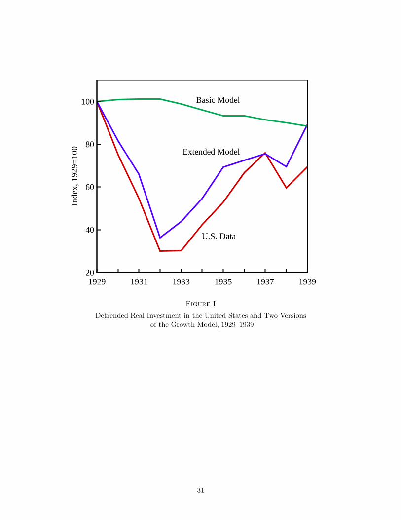
Figure I establishes my main result, namely, that abstracting from key features of U.S. fiscal

policy makes a big difference in the model’s prediction of real investment as measured in NIPA.11

In the basic version of the model, with only taxes on profits and wages included, real investment

rises 2 percent relative to trend between 1929 and 1932 and eventually falls by 2 percent. On the

other hand, the extended model predicts an immediate and sharp fall in investment, much like

that in the U.S. economy. In both the extended model and the data, declines occur in the period

1929–1932 and then again in 1938.

The fact that investment falls and tax rates rise also has implications for equity values. The

11 The conclusion does not change if, in the basic model, I use Joines’ (1981) tax rates—as Cole and Ohanian(1999) do—or add a nonbusiness sector. See McGrattan (2012).

13

predicted value is shown in equation (6). With a rise in tax rates, prices and quantities fall, but

the model predicts more gradual changes than those of actual stock market values. For example,

the real market value of all stocks traded on the New York Stock Exchange fell 57 percent below

trend between 1929 and 1932 and by 1939 was below trend by 32 percent. (See U.S. Commerce,

1932–1950.) The model does predict a significant decline between 1929 and 1939, reaching a low

of 30 percent below trend, but the drop is gradual because the changes in tax rates and capital

stocks are gradual. By 1932, predicted stock values are only 12 percent below trend.

Figure II shows the consumption paths for the basic and extended models in comparison with

U.S. data. Neither model does well in predicting real consumption, but the extended model does

a bit better. In the data, real consumption drops sharply relative to trend and stays close to its

1933 low through the rest of the decade. In the basic model, consumption barely changes from

its 1929 level. In the extended model, the consumption path counterfactually rises before 1932.

The optimal response to high future capital taxes is high current distributions of business capital,

which are used for consumption.12 According to Fabricant (1935), U.S. dividend payments held

steady at the start of the Depression, even for many companies suffering losses, but the model

predicts an increase. Taxes on consumption do rise during the 1930s, implying a negative impact

on consumption, but not significantly until after 1932. At that point, consumption in the extended

model does decline sharply.

Predictions for real GDP are shown in Figure III. Not surprisingly, given the predictions for

investment and consumption, neither of the models accounts for the full fall in observed GDP. But

the extended model shows a large improvement over the basic model prediction, which has the

wrong sign. The basic model predicts a 1 percent rise in detrended real GDP between 1929 and

1932, rather than a 31 percent fall. This prediction is the basis of conventional wisdom that fiscal

policy can be safely ignored. The extended model, however, predicts an initial decline in real GDP

that is about 36 percent of the actual decline. The decline in model GDP is not greater because

households consume more in the early part of the decade when businesses increase distributions.

Figure IV shows hours worked per capita for the basic and extended models along with the

U.S. data. As in the case of GDP, the prediction of the basic model has the wrong sign. The basic

model predicts a 2 percent rise in per capita hours of work between 1929 and 1932, rather than a

27 percent fall. Households work more because labor income tax rates actually fall in the first part

12 The large deviation between consumption patterns in theory and data cannot be resolved by introducing thetype of financial frictions proposed by Bernanke and Gertler (1989). Taxes on dividends and undistributedprofits have the same impact on economic activity as the agency costs in their model. Both impact the priceof capital, leading to declines in investment and increases in consumption.

14

of the Depression, and taxes on business profits have little impact on labor inputs in this period.

The extended model, however, predicts an initial decline in hours of work that is about 38 percent

of the actual decline. This decline occurs even though the tax rate on labor income falls initially

because other taxes that impact hours of work are included in the analysis.

Overall, the results show that the extended model’s predictions for the impact of U.S. fiscal

policy are greater than those of the basic model. And the impact is nontrivial, especially for

investment. This overturns the standard result that fiscal policy played little or no role in the

U.S. Great Depression.

V. Investigating the Main Results

To better understand the contributions of the various factors included in the extended model,

I simulate variants of the model. The first set of simulations, with all but the key factors held

constant over time, provide intuition. The second set of simulations, with perturbations of the

benchmark parameterization, provide a sense of the quantitative impact of the key factors. Overall,

the experiments demonstrate that the primary factors driving the results are taxes on dividends

in the early part of the decade and taxes on undistributed profits in the latter part. The choice of

expectations does affect the pattern of the investment series but, within an empirically plausible

range, does not overturn the main conclusions. Finally, I show that including factors specifically

intended to generate patterns of GDP and hours consistent with those observed does not worsen

the fit of investment.13

V.A. The Key Factors

In this section, I investigate three key factors for the results and the role each plays in gen-

erating the large decline in investment predicted by the extended model. (See Figure I.) The first

two are the tax rates on dividends and undistributed profits.14 The third is expectations about

future tax rates on dividends and undistributed profits.

The primary determinant for the predicted fall in investment in the early 1930s is expectations

about future changes in the tax rate on dividends. The reason for the large decline is that firms

anticipate large changes in the effective return to capital. To see this, consider the households’

13 See McGrattan (2012) for additional experiments and sensitivity analyses.14 In McGrattan (2012) I do sensitivity analysis with the other taxes and find that the taxes on distributed and

undistributed profits are quantitatively most important.

15

intertemporal first-order condition for capital when nonnegativity constraints are not binding on

investment:

(7)(1+τut) (1−τdt)

(1 + τct) ct= βEt

[ (1−τdt+1)

(1+τct+1) ct+1

{(1−τpt+1) (rt+1−δ−τkt+1)+1+τut+1}]

,

where expectations are conditioned on the state st, β = β/(1 + γ), and variables with hats are

per capita series detrended by technology growth; for example, ct = ct/(1 + γ)t.15 If tax rates on

dividends are constant, then the terms 1−τdt and Et(1−τdt+1) cancel. If, in addition, revenues are

lump sum rebated to households, then taxes on dividends have no effect on equilibrium quantities

other than equity values because neither budget sets nor first-order conditions change. However,

if households put a positive probability on dividend tax rates changing, then these taxes do affect

the equilibrium quantities. As soon as there is any weight put on the possibility of a future rise in

income tax rates, firms increase current distributions to households by lowering investment. Once

tax rates start to rise, they decrease distributions and hence increase their investment, implying a

V-shaped pattern for investment.16

To provide intuition for the qualitative results, I consider a simple example with the tax rate

on dividends starting at a low level, say τLd , and eventually rising to a higher level, τH

d > τLd .

For now, assume that all other exogenous processes remain fixed and the only variables are the

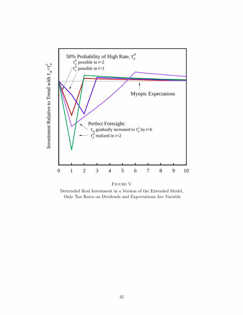
dividend tax rate and expectations about the future dividend tax rates. Figure V shows several

paths of investment for different choices of expectations and realizations. In all cases, the rate is

τLd at t=0 and, at that date, is expected to persist. In t=1, expectations change. Consider first the

case of perfect foresight with the high tax rate realized one period later. At t=1, there is a sharp

drop in investment relative to its growth trend. Firms distribute earnings when the tax rate is still

low, knowing for sure that it will be high in the next period. If the higher tax rate is gradually

phased in over time, which is the case for the path marked τdt gradually increased, then the drop

at t=1 is less severe, but investment stays below trend until τdt = τHd . For the path shown, the

tax rate increases linearly, starting at τLd in t=1 and rising to τH

d in t=6, and then stays high

thereafter.

Suppose instead of assuming that households have perfect knowledge of the entire future path

of tax rates, I assume there is some uncertainty about future rates. For the two cases marked 50%

15 Intuition for the actual simulation is complicated by the fact that negativity constraints do bind in some statesof the world.

16 In a study of the U.S. Jobs and Growth Tax Relief Reconciliation Act of 2003, Chetty and Saez (2005) provideempirical evidence that cuts in dividend taxes have large and immediate effects on payout policies of firmswith high levels of taxable noninstitutional ownership.

16

Probability of High Rate in Figure V, the tax rate is low in t=1, but households now realize that an

increase is possible. The fact that an increase is possible is all that is needed to trigger a drop in

investment, because households and firms want to take advantage of the current low rate. The fall

in investment occurs regardless of whether the tax rate is increased. In the first case, τHd possible

in t=2, uncertainty is resolved in one period: with 50 percent probability rates stay low and with

50 percent probability rates rise and stay high. Whether the high rate is in fact realized in t=2 is

irrelevant: the pattern is the same because the rate is expected to remain constant thereafter. If

I increase the probability of a tax increase in the next period, say from 50 percent to something

closer to 100 percent, then the equilibrium path is closer to that of the perfect foresight; this is

true even if the higher rate is never realized. Again, what matters is the expected change in the

rate.

Delaying the resolution of uncertainty changes the initial pattern somewhat. In the case

marked τHd possible in t=3, uncertainty is not fully resolved until t=3. In t=1, there is a 50 percent

chance that the tax rate remains permanently low starting in t ≥ 2 and a 50 percent chance that

the tax rate is low again in t=2 but could increase after that. Investment falls immediately and

continues to fall until the uncertainty is resolved. As before, the path does not depend on the

realization of a high rate occurring in t=3. The expectations of higher rates drive the fall in

investment.

The last simulation shown in Figure V assumes that households have myopic expectations: the

rate next period is expected to be equal to the current rate. Although this scenario is implausible

for the Great Depression, given the many news reports about looming deficits in the early 1930s,

the experiment shows what is needed for no change in investment relative to its trend. What is

not determinate in this case is the path of tax rates: any arbitrary sequence of dividend tax rates

is consistent with the fixed path of investment when expectations are myopic. If households and

firms expect no change, they do not react by adjusting their investments and distributions.

A second key tax rate in the analysis is the tax on undistributed profits, which was introduced

during the Great Depression in 1936. The first-order condition in equation (7) shows that a positive

tax on undistributed profits distorts the intertemporal investment decision. Unlike the tax rate

on distributed profits, the tax rate on undistributed profits has an impact on investment and the

stock of capital even if it is expected to remain constant.

In Figure VI, I display several simulations that highlight the impact of undistributed profits

taxes on investment as I vary expectations. In all cases, I assume that the tax increase is temporary

17

as it was in the United States; the rate is temporarily high in the second and third periods. In the

first simulation, expectations are perfect and therefore investment rises prior to the tax increase

as firms anticipate the rate change. Then, once taxes are high, investment drops. Investment

recovers once the tax rate is back to zero, rising slightly above trend and eventually returning to

trend. If firms are surprised by the increase in taxes and think the rate will be equal to zero in

the next period, then there is no initial increase, but the two-period decline when the tax is in

place is similar to the perfect foresight path. If expectations are myopic, so changes are a surprise

and viewed as permanent, the pattern of investment is the same as in the other two simulations,

although investment does not fall as much in the high tax periods. Investment does not fall more

when expectations are myopic because firms view the rate increase as permanent.

With this result in mind, it is possible to construct an example in which the investment does

not fall at all and may even rise in high tax periods. Firms may expect future tax rates to be

even higher than they are currently and to remain at that higher level permanently. In this case,

two offsetting effects occur: the higher realized rates impact current investment negatively, but

higher expected future rates impact current investment positively. Whether investment falls or

rises depends on the relative magnitudes of the realized tax rates and the expected future tax

rates.

V.B. Variations in the Benchmark Simulations

Thus far, I have considered the qualitative nature of the results. Next, I consider simulations

starting with the benchmark (shown in Figures I–IV) to investigate the quantitative impact of the

key factors. In all cases, I restrict attention to predictions for investment. (See McGrattan, 2012,

for plots of the other series.)

In Figure VII, I show the consequences of setting the tax rates on dividends and undistributed

profits to zero in the benchmark simulation. If the tax rate on dividends is equal to zero, the model

cannot account for the dramatic decline in investment that occurred between 1929 and 1932. In

this case, the tax rate tomorrow equals the tax rate today and the impact on capital is negligible.

The results in Figure VII are not altered if instead of setting the tax rate on dividends to zero, I

set it equal to any constant. As I showed earlier, what matters is the expectation of next period’s

tax rate relative to today’s.

The fact that the tax rate on dividends has a much larger impact on investment than the

tax rate on profits is best understood by again examining the households’ intertemporal first-order

condition in equation (7). Tax rates on profits lower the net return on capital, r − δ − τk. Tax

18

rates on dividends, if expected to change, lower the gross return on capital, which is equal to 1+τu

plus the after-tax net return.17 Net returns are on the order of 4 percent, and therefore even large

changes in the tax rate on profits cannot have a large impact on the gross return. On the other

hand, because they impact the gross return, even small changes in the tax rates on dividends can

have a quantitatively large impact, as long as they are not completely unexpected.

The second simulation shown in Figure VII is the case with the undistributed profits tax set to

zero. If the tax rate on undistributed profits is counterfactually set to zero in 1936–1938, then the

model cannot account for the recession of 1937–1938. The tax motivates companies to temporarily

decrease retained earnings and distribute more. For example, the no-tax version of the model

predicts distributions in 1936 and 1937 that are higher by about 33 and 43 percent relative to the

benchmark model predictions, respectively.18

In Figure VIII, I show how the quantitative results for the benchmark simulation depend on

household expectations about fiscal policy changes. To do this, I compute the extended model’s

equilibrium for three alternative assumptions about these expectations. One is the benchmark

set of assumptions used in the initial simulation. A second assumes that in 1930, households

put the probability of staying with 1930 policy for another year at 100 percent; the same can

be said for 1931. The transition matrix for 1932 and after is the same as in Table II. I call this

alternative Myopic Expectations, 1930–1931. The third alternative is to assume perfect foresight,

that households have full knowledge of the path of spending and tax rates. I call this alternative

Perfect Foresight, 1930–1939.

As is clear in Figure VIII, the model’s predictions of investment do seem different with the

three alternative assumptions. If households place no probabilistic weight on the higher tax rates of

the 1930s, as is true in the case myopic expectations, then investment does not fall initially as much

as it does in the benchmark. If households have perfect foresight, then they react immediately and

sharply to the news by setting business investment close to zero. However, in all cases, there is a

first-order effect on investment and one much larger than the basic growth model prediction.

Another difference worth noting about the experiments shown in Figure VIII is the reaction

17 Consumption taxes also impact the gross returns to capital, but they are not equivalent to dividend taxesbecause they affect the households’ intratemporal first-order condition as well. It is easy to show the equiv-alence between the extended model and an alternative without dividend taxes. In the alternative, taxes onconsumption and labor are set as follows: τct = (1 + τct)/(1− τdt)− 1 and τht = 1− (1− τht)/(1− τdt), whereτct, τht, and τdt are tax rates in the original model.

18 Lent (1948) estimates the extent to which the policy impacted distributions by computing deviations of thecorrelation between dividend payments and after-tax profits from trend based on data for 1934–1942, excluding1936 and 1937. From these deviations, he predicts that net dividend payments are higher in both 1936 and1937 by about 24 percent.

19

to news about the undistributed profits tax. In the benchmark simulation, this tax is completely

unanticipated. In the perfect foresight case, it is completely anticipated. Thus, investment sharply

rises between 1931 and 1935 and falls when the tax is in effect.

Clearly, factors other than tax policy were involved in depressing consumption and GDP at

the start of the Depression and hours of work throughout the decade. I next show that adding

exogenous efficiency and labor wedges—shocks to productivity and tax rates on labor intended to

generate dynamics of GDP and hours of work equivalent to U.S. patterns—does not worsen the fit

of investment. Specifically, I allow for variations in Zt and τht that generate a perfect fit between

the equilibrium paths of GDP and hours in the extended model and in the data.19 I then compare

investment in the model and data to see if it looks much different from the benchmark simulation

in Figure I.

The exercise shows that the pattern for investment is, if anything, closer to the actual pattern.

This pattern is evident in Figure IX, which plots total investment for the mdoel with and without

exogenous wedges. The inclusion of efficiency wedges that act like negative productivity shocks

further depresses investment. However, the impact is not as large as it is for consumption and

output because investment is already close to zero in 1932 and is constrained to be nonnegative

in equilibrium. Thus, the fit of investment is not worsened when the additional factors depressing

the economy are included.

VI. Cross-Country Evidence

My results are broadly supported by evidence on changes in income tax rates and GDP in

other countries during the 1930s.20 Countries had a wide range of experiences during the 1930s.

Some countries had little or no decline in economic activity, and some, like the United States, had

dramatic declines. Although to the best of my knowledge, tax data are insufficient for countries

outside of the United States to conduct the same analysis as above, I do have information about

tax schedules and real per capita GDPs during this period. The information is suggestive that

countries with the largest increases in income tax rates were also the most depressed.

In Table III, I report the top marginal tax rates in 1929 and 1935 for seven countries that had

significantly different experiences in the 1930s. A preferable measure would be the average marginal

19 As Chari, Kehoe, and McGrattan (2007) emphasize, the challenge is to find primitive shocks and mechanismsthat have the same impact as these time-varying efficiency and labor wedges.

20 In McGrattan (2012), I also analyze predictions of the model for other time periods in the United States.

20

tax rate on dividends, but the necessary underlying data for this measure—namely, marginal tax

rates and dividend income by income class—are not publicly available for any country but the

United States in this period. Thus, as a proxy for the change in the average marginal tax rate on

dividends, I use the change in the top marginal rate on dividend income, since most dividends are

earned by households in high income classes. Along with tax rates, I report the deviation in per

capita real GDP relative to a growth trend of 1.9 percent per year for the year 1933. Figure X

shows the time series of detrended real GDP for Sweden, the United Kingdom, France, Australia,

New Zealand, the United States, and Canada. Numbers in parentheses are the differences in the

top marginal tax rates listed in Table III.21

These data show that there is a strong negative correlation, roughly −94 percent, between the

change in the top income tax rates and the deviation in per capita real GDP relative to trend in

1933. As noted above, what matters is the change in the tax rates, not the levels. Thus, the fact

that the United Kingdom had high tax rates in this period is not relevant for the theory. What is

relevant is that their tax policies changed little.

VII. Conclusion

Many theories have been proposed for the large contraction of the 1930s and the slow recovery

thereafter. Absent from the theories of Friedman and Schwartz (1963), Bernanke and Gertler

(1989), Cole and Ohanian (2004), Ohanian (2009), and many others is any role for fiscal policy

in this decade. This paper challenges the conventional view that fiscal policy played little or no

role in the Great Depression. Government spending and a variety of tax rates rose significantly

during this decade, or were expected to, and theory tells us that these events should have had an

impact. Especially important are the sharp rise in tax rates on individual incomes, which include

dividend income, and the introduction of the undistributed profits tax. Large changes in tax rates

on dividends, when fed into the neoclassical growth model, imply a large drop in investments,

similar to what we observed at the start of the 1930s. In the later part of the 1930s, tax rates on

undistributed profits were introduced and led to another dramatic decline in investment.

Although the results show that capital taxation during the U.S. Great Depression had large

effects, it cannot be the only overlooked factor in the analysis of the period. If the only change

21 Sources for the income tax rate schedules are the U.S. Treasury (1916–2010) for the United States, the Com-monwealth of Australia (1932, 1942–1943) for Australia, Tolley (1938) for the United Kingdom, the CanadianTax Foundation (1957) for Canada, Steinmo (1996) for Sweden, Piketty (2001) for France, and Vosslamber(2010) for New Zealand.

21

is a rise in tax rates, theory predicts that consumption counterfactually rises before 1932, with

households anticipating some increases in income taxes and sales taxes. This deviation is also

evident in standard theories of financial frictions and remains a challenge for those interested in

accounting for the dramatic contraction in the early 1930s.

Appendix

The main source for the national accounts data used in this study is the U.S. Department

of Commerce, Bureau of Economic Analysis (BEA), which publishes the U.S. national accounts

and fixed asset tables in the Survey of Current Business (available online at www.bea.gov), SCB

hereafter. The main source for hours data is Kendrick (1961). In this appendix, I provide details

on these data and the necessary adjustments that are made to make the model accounts consistent

with the U.S. accounts.

A. National Accounts and Fixed Assets

The main components of GDP are found in Table 1.1.5 of the national income and product

accounts (NIPA) from the SCB (1929–2011). GDP in the business sector is set equal to value

added of corporations and nonfarm proprietorships. Nonbusiness output is residually defined as

GDP less business value added.

B. Components of GDP

Components of GDP used as inputs in the quantitative analysis are shown in Table A.1.

Private consumption is defined to be personal consumption expenditures on nondurables and ser-

vices, adjusted to include consumer durable services and to exclude sales tax. (Details of these

adjustments are described below.) Investment is defined to be the sum of gross private domes-

tic investment, government investment, net exports, and personal consumption expenditures on

durables after subtracting sales taxes. Business investment is defined to be the part of investment

made by corporations and nonfarm proprietors. Nonbusiness investment is residually defined as

investment less business investment. Government spending is defined to be government consump-

tion expenditures. In Table A.1, this spending is listed as public consumption to distinguish it from

private consumption. All components of GDP are deflated by the GDP deflator (in NIPA Table

1.1.9) and population at midperiod (NIPA Table 2.1). The series are then divided by the growth

in labor-augmenting technical change (1 + γ)t.

Components of GDP treated exogenously and used as inputs in the model simulations—

namely, detrended government spending and detrended nonbusiness activities—are filtered using

the algorithm proposed by Hodrick and Prescott (1997). I set their smoothing parameter (λ) equal

to 1. The unfiltered series are displayed in Table A.1. The same smoothing procedure is used for

22

the tax series displayed in Table I. In a separate technical appendix (McGrattan, 2012), I plot all

of the smoothed inputs along with the original time series.

C. Adjustments to Accounts

Two adjustments are made to GDP and its components to make them consistent with the

model accounts: sales taxes are subtracted, and services for consumer durables and government

capital are added.

Unlike the NIPA, the model output does not include consumption taxes as part of consumption

and as part of value added. I therefore subtract sales and excise taxes from the NIPA data on

taxes on production and imports and from personal consumption expenditures, since these taxes

primarily affect consumption expenditures.

I treat expenditures on all fixed assets as investment. Thus, spending on consumer durables

is treated as an investment rather than as a consumption expenditure and moved from the con-

sumption category to the investment category. The consumer durables services sector is introduced

in the same way as the NIPA introduces owner-occupied housing services. Households rent the

consumer durables to themselves. Specifically, I add depreciation of consumer durables to con-

sumption of fixed capital of households and to private consumption. I add imputed additional

capital services for consumer durables to capital income and to private consumption. I assume

a rate of return on this capital equal to 4.1 percent, which is an estimate of the return on other

types of capital. A related adjustment is made for government capital. Specifically, I add imputed

additional capital services for government capital to capital income and to public consumption.

D. Hours Per Capita

The primary source of the hours series in Table A.1 is Kendrick (1961), Table A-X, total

manhours. Nonbusiness hours are the sum of hours in the government and farm sectors. Business

hours are total hours less nonbusiness hours. For per capita hours, I divide the manhours series

by the working-age population, defined to be age 16 and over. The population series is Series A39

of the Historical Statistics of the U.S. Department of Commerce (1975).

Federal Reserve Bank of Minneapolis

University of Minnesota

National Bureau of Economic Research

Supplementary Material

Supplementary material is available at The Quarterly Journal of Economics online.

23

References

Bakija, Jon. “Documentation for a Comprehensive Historical U.S. Federal and State Income Tax

Calculator Program,” Williams College, 2009.

Barro, Robert J., and Charles J. Redlick. “Macroeconomic Effects from Government Purchases

and Taxes,” Quarterly Journal of Economics, 126 (2011), 51–102.

Barro, Robert J., and Chaipat Sahasakul. “Measuring the Average Marginal Tax Rate from the

Individual Income Tax,” Journal of Business, 56 (1983), 419–452.

. “Average Marginal Tax Rates from Social Security and the Individual Income Tax,” Jour-

nal of Business, 59 (1986), 555–566.

Bernanke, Ben, and Mark Gertler. “Agency Costs, Net Worth, and Business Fluctuations,” Amer-

ican Economic Review, 79 (1989), 14–31.

Braun, R. Anton. “Tax Disturbances and Real Economic Activity in the Postwar United States,”

Journal of Monetary Economics, 33 (1994), 441–462.

Brown, E. Cary. “Some Evidence on Business Expectations,” Review of Economics and Statistics,

31 (1949), 236–238.

. “Fiscal Policy in the ’Thirties: A Reappraisal,” American Economic Review, 46 (1956),

857–879.

California Franchise Tax Commissioner. Personal Income Tax: Statistics of 1938 Returns, unpub-

lished volume, California Franchise Tax Board, 1940.

Calomiris, Charles W., and R. Glenn Hubbard. “External Finance and Investment: Evidence from

the Undistributed Profits Tax of 1936,” Journal of Business, 68 (1995), 443–482.

Canadian Tax Foundation. Canadian Fiscal Facts (Toronto: Canadian Tax Foundation, 1957).

Chari, V.V., Patrick J. Kehoe, and Ellen R. McGrattan. “Business Cycle Accounting,” Economet-

rica, 75 (2007), 781–836.

Chetty, Raj, and Emmanuel Saez. “Dividend Taxes and Corporate Behavior: Evidence from the

2003 Dividend Tax Cut,” Quarterly Journal of Economics, 120 (2005), 791–833.

Cole, Harold L., and Lee E. Ohanian. “The Great Depression in the United States from a Neoclas-

sical Perspective,” Federal Reserve Bank of Minneapolis Quarterly Review, 23 (1999), 2–24.

. “New Deal Policies and the Persistence of the Great Depression: A General Equilibrium

Analysis,” Journal of Political Economy, 112 (2004), 779–816.

Commonwealth of Australia, Bureau of Census and Statistics. Fourteenth Report of the Commis-

sioner of Taxation (Canberra: Commonwealth Government Printer, 1932).

. Official Year Book of the Commonwealth of Australia, No. 35 (Canberra: Commonwealth

Government Printer, 1942–1943).

24

Fabricant, Solomon. Profits, Losses and Business Assets, 1929–1934, National Bureau of Economic

Research, Bulletin 55, 1935.

Feenberg, Daniel, and Elisabeth Coutts. “An Introduction to the TAXSIM Model,” Journal of

Policy Analysis and Management, 12 (1993), 189–194.

Friedman, Milton, and Anna Jacobson Schwartz. A Monetary History of the United States, 1867–

1960 (Princeton, NJ: Princeton University Press, 1963).

Goldsmith, Raymond W. Financial Intermediaries in the American Economy since 1900 (Prince-

ton, NJ: Princeton University Press, 1958).

Haven, T. Kenneth. “Investment Banking under the Securities and Exchange Commission,” Michi-

gan Business Studies, 9 (1940), 1–157.

Hodrick, Robert J., and Edward C. Prescott. “Postwar U.S. Business Cycles: An Empirical

Investigation,” Journal of Money, Credit, and Banking, 29 (1997), 1–16.

Holland, Daniel M. Dividends Under the Income Tax (Princeton, NJ: Princeton University Press,

1962).

Joines, Douglas H. “Estimates of Effective Marginal Tax Rates on Factor Incomes,” Journal of

Business, 54 (1981), 191–226.

Kehoe, Timothy J., and Edward C. Prescott. Great Depressions of the Twentieth Century (Min-

neapolis, MN: Federal Reserve Bank of Minneapolis, 2007).

Kendrick, John W. Productivity Trends in the United States (Princeton, NJ: Princeton University

Press, 1961).

Lent, George E. The Impact of the Undistributed Profits Tax, 1936-1937 (New York, NY: Columbia

University Press, 1948).

McGrattan, Ellen R. “The Macroeconomic Effects of Distortionary Taxation,” Journal of Monetary

Economics, 33 (1994), 573–601.

. “Technical Appendix: Capital Taxation During the U.S. Great Depression,” Federal Re-

serve Bank of Minneapolis, Staff Report 452, 2012.

Ohanian, Lee E. “What — or Who — Started the Great Depression?” Journal of Economic

Theory, 144 (2009), 2310–2335.

Piketty, Thomas. Les Hauts Revenus en France au 20e siecle: Inegalites et Redistribution, 1901–

1998 (Paris: B. Grasset, 2001).

Securities and Exchange Commission. Statistical Release no. 572 (Washington, DC: Securities and

Exchange Commission, 1941).

Seltzer, Lawrence H. “Quantitative Aspects of the Role of the Exemptions and Associated Factors

in Expanding the Coverage and Yield of the Income Tax,” in The Personal Exemptions in the

Income Tax, Lawrence H. Seltzer, ed. (New York, NY: National Bureau of Economic Research,

1968).

25

Steinmo, Sven. Taxation and Democracy: Swedish, British and American Approaches to Financing

the Modern State (New Haven, CT: Yale University Press, 1996).

Tax Research Foundation. Federal and State Tax Systems (Chicago, IL: Commerce Clearing House,

1930–1933).

. Tax Systems of the World (Chicago, IL: Commerce Clearing House, 1934–1938).

. Tax Systems (Chicago, IL: Commerce Clearing House, 1940–1942).

Tolley, Charles H. Tolley’s Complete Income Tax, Sur-Tax, etc., Chart-Manual of Rates, Al-

lowances and Abatements (London, UK: Waterlow, 1938).

U.S. Commerce, Department of Commerce, Bureau of the Census. Historical Statistics of the

United States: Colonial Times to 1970, Bicentennial ed. (Washington, DC: U.S. Government

Printing Office, 1975).

U.S. Commerce, Department of Commerce, Bureau of Economic Analysis. Survey of Current

Business (Washington, DC: U.S. Government Printing Office, 1929–2011).

. Survey of Current Business: Annual Supplements (Washington, DC: U.S. Government

Printing Office, 1932–1950).

U.S. Treasury, Department of the Treasury, Bureau of Internal Revenue. Statistics of Income

(Washington, DC: U.S. Government Printing Office, 1916–2010).

. The Audit Control Program: A Summary of Preliminary Results (Washington, DC: U.S. Gov-

ernment Printing Office, 1948).

Vosslamber, Robert J. “Taxing and Pleasing: The Rhetoric and Reality of Vertical Equity in

the Development of the New Zealand Income Tax on Employees, 1891–1984,” Ph.D. thesis,

University of Canterbury, Christchurch, New Zealand, 2010.

26

Table I

U.S. Tax Rates, 1929–1939

Individual Income Corporate Profits Indirect Business

Year Labor Dividend Normal Excessa Undistributed Property Sales

1929 3.60 9.51 11.00 −− −− 1.41 2.89

1930 2.40 7.90 12.00 −− −− 1.63 2.99

1931 1.80 7.71 12.00 −− −− 1.60 3.40

1932 3.00 14.13 13.75 −− −− 1.99 3.98

1933 3.20 14.41 13.75 2.00 −− 1.84 5.92

1934 3.60 16.70 13.75 2.00 −− 1.74 6.97

1935 4.10 19.09 13.75 2.00 −− 1.73 7.05

1936 5.50 25.04 15.00 2.00 5.00 1.71 6.90

1937 5.80 24.97 15.00 2.00 5.00 1.69 7.08

1938 4.60 20.23 19.00 2.00 5.00 1.59 7.10

1939 5.10 21.83 19.00 2.00 −− 1.62 7.19

a. in combination with the capital stock tax.

27

Table II

Transition Matrix for Benchmark Model Simulation

Policy Next Period’s Policy Like That ofTodayLike 1929 1930 1931 1932 1933 1934 1935 1936 1937 1938 1939

1929 1

1930 1

3

1

3

1

3

1931 1

3

1

3

1

3

1932 1

1933 1

1934 1

1935 1

1936 2

3

1

3

1937 2

3

1

3

1938 1

1939 1

28

Table III

Changes in Tax Rates and Real GDP in Seven Countries

Top Marginal Income Tax Rates (%) 1933 Per Capita Real GDP

1929 1935 Difference Relative to Trend

Country (1) (2) (2)−(1) (percent)

Sweden 30.2 35.4 5.2 −10.8

United Kingdom 57.5 63.8 6.3 −11.1

France 41.7 50.4 8.7 −16.5

Australiaa 27.0 42.5 15.5 −14.7

New Zealanda 22.5 39.0 16.5 −19.3

United Statesa 20.0 59.0 39.0 −35.8

Canadaa 40.0 69.3 29.3 −38.3

a. Rates differ by type of income. Table reports rates on dividend income.

29

Table A.1

U.S. National Accounts and Hours of Work, 1929–1939

Consumption Aggregate Activity Nonbusiness Activity

Year Private Public GDP Investment Hours Output Investment Hours

1929 68.1 5.8 100.0 26.1 28.9 36.9 15.0 7.4

1930 63.3 6.1 89.0 19.6 26.6 33.2 12.1 7.3

1931 60.4 6.7 81.4 14.3 24.2 33.5 11.0 7.3

1932 54.3 7.1 69.2 7.8 21.2 30.8 7.4 7.0

1933 51.1 7.2 66.4 7.9 21.0 30.4 6.5 7.1

1934 51.6 7.8 70.4 11.0 20.8 29.3 7.3 6.8

1935 52.8 7.7 74.3 13.8 21.6 30.6 9.6 7.0

1936 56.0 8.3 81.8 17.4 23.3 32.5 10.6 7.3

1937 56.0 7.8 83.6 19.8 24.0 32.0 12.3 7.3

1938 54.8 8.3 78.5 15.6 22.1 31.9 12.0 7.1

1939 55.5 8.7 82.5 18.1 22.8 32.3 12.8 7.0

Notes: GDP and components are in real per capita terms and divided by an annual growth trend of 1.019t.

These series are further divided by the 1929 level for per capita real GDP. Hours are in per capita terms and divided

by 5,000, which is an estimate of annual discretionary hours. Finally, all series are multiplied by 100.

30

Inde

x, 1

929=

100

1929 1931 1933 1935 1937 193920

40

60

80

100

U.S. Data

Basic Model

Extended Model

Figure I

Detrended Real Investment in the United States and Two Versions

of the Growth Model, 1929–1939

31

Inde

x, 1

929=

100

1929 1931 1933 1935 1937 193970

80

90

100

110

U.S. Data

Basic Model

Extended Model

Figure II

Detrended Real Consumption in the United States and Two Versions

of the Growth Model, 1929–1939

32

Inde

x, 1

929=

100

1929 1931 1933 1935 1937 193960

70

80

90

100

110

U.S. Data

Basic Model

Extended Model

Figure III

Detrended Real GDP in the United States and Two Versions

of the Growth Model, 1929–1939

33

Inde

x, 1

929=

100

1929 1931 1933 1935 1937 193970

80

90

100

U.S. Data

Basic Model

Extended Model

Figure IV

Hours Worked Per Capita in the United States and Two Versions

of the Growth Model, 1929–1939

34

Inve

stm

ent R

elat

ive

to T

rend

with

τdt=

τ dL

0 1 2 3 4 5 6 7 8 9 10

50% Probability of High Rate, τdH

Perfect Foresight:

Myopic Expectations

τdH possible in t=2

τdH possible in t=3

τdt gradually increased to τdL by t=6

τdH realized in t=2

Figure V

Detrended Real Investment in a Version of the Extended Model,

Only Tax Rates on Dividends and Expectations Are Variable

35

Inve

stm

ent R

elat

ive

to T

rend

with

τut=

0

0 1 2 3 4 5 6 7 8 9 10

Always Expect τu,t+1=0

Perfect Foresight

Myopic Expectations

Figure VI

Detrended Real Investment in a Version of the Extended Model,

Only Tax Rates on Undistributed Profits and Expectations Are Variable

Note: In all cases, rates are only positive in t=2 and t=3.

36

Inde

x, 1

929=

100

1929 1931 1933 1935 1937 193920

40

60

80

100

Benchmark

τdt = 0

τut = 0

U.S. Data

Extended Model:

Figure VII

Detrended Real Investment in the United States and in the Extended

Model, 1929–1939, with Alternative Assumptions for Capital Taxes

37

Inde

x, 1

929=

100

1929 1931 1933 1935 1937 193920

40

60

80

100

Benchmark

Myopic Expectations, 1930−1931

Perfect Foresight, 1930−1939

U.S. Data

Extended Model:

Figure VIII

Detrended Real Investment in the United States and in the Extended

Model, 1929–1939, with Alternative Assumptions for Expectations

38

Inde

x, 1

929=

100

1929 1931 1933 1935 1937 193920

40

60

80

100

Benchmark

Exogenous Wedges Added

U.S. Data

Extended Model:

Figure IX

Detrended Real Investment in the United States and in the Extended

Model, 1929–1939, with Exogenous Wedges Added

39

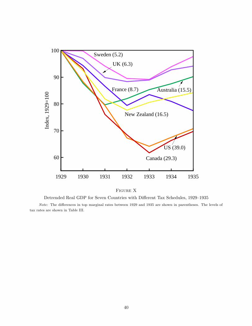
Inde

x, 1

929=

100

1929 1930 1931 1932 1933 1934 1935

60

70

80

90

100Sweden (5.2)

UK (6.3)

France (8.7)

New Zealand (16.5)

US (39.0)

Canada (29.3)

Australia (15.5)

Figure X

Detrended Real GDP for Seven Countries with Different Tax Schedules, 1929–1935

Note: The differences in top marginal rates between 1929 and 1935 are shown in parentheses. The levels of

tax rates are shown in Table III.

40