Capture Point: A Step toward Humanoid PushRecovery

Jerry Pratt, John Carff, Sergey DrakunovFlorida Institute for Human and Machine Cognition

Pensacola, Florida 32502Email: jpratt@ihmc.us

Ambarish GoswamiHonda Research Institute

Mountain View, California 94041Email: agoswami@honda-ri.com

Abstract— It is known that for a large magnitude push ahuman or a humanoid robot must take a step to avoid a fall.Despite some scattered results, a principled approach towards“When and where to take a step” has not yet emerged.

Towards this goal, we present methods for computing CapturePoints and the Capture Region, the region on the ground wherea humanoid must step to in order to come to a complete stop.The intersection between the Capture Region and the Base ofSupport determines which strategy the robot should adopt tosuccessfully stop in a given situation.

Computing the Capture Region for a humanoid, in general, isvery difficult. However, with simple models of walking, compu-tation of the Capture Region is simplified. We extend the well-known Linear Inverted Pendulum Model to include a flywheelbody and show how to compute exact solutions of the CaptureRegion for this model. Adding rotational inertia enables thehumanoid to control its centroidal angular momentum, muchlike the way human beings do, significantly enlarging the CaptureRegion.

We present simulations of a simple planar biped that canrecover balance after a push by stepping to the Capture Regionand using internal angular momentum. Ongoing work involvesapplying the solution from the simple model as an approximatesolution to more complex simulations of bipedal walking, includ-ing a 3D biped with distributed mass.

I. INTRODUCTION

Push recovery is important for humanoid robots operatingin human environments. No matter how well we attempt toshield these robots, it is inevitable that they will occasionallybump into objects and other people, and will be tripped upby debris, rocks, and objects that go undetected. Therefore,their ultimate utility will depend on good algorithms for pushrecovery.

Like most aspects of bipedal walking, push recovery isdifficult because bipedal walking dynamics are high dimen-sional, non-linear, and hybrid. Moreover, a humanoid robotis underactuated and makes friction-limited unilateral contactswith the ground. Despite these theoretical difficulties, animalsand humans are very adept at push recovery. As the push forceprogressively grows larger, strategies that they use includemoving the Center of Pressure within the foot, accelerating in-ternal angular momentum through lunging and “windmilling”of appendages, and taking a step. Although the humanoidliterature contains several analysis and control techniques foreach strategy, there is yet to emerge a principled approachtowards “when and where to step” under a force disturbance.

This paper seeks to contribute in this direction using theconcept of Capture Points.

A Capture Point is a point on the ground where the robot canstep to in order to bring itself to a complete stop. A CaptureRegion is the collection of all Capture Points. Fast and accuratecomputation of Capture Points may be difficult and closedform solutions might not exist for a general humanoid robot.In this paper we examine simple models of walking that canbe used to explain push recovery strategies, and to developalgorithms for implementing these strategies on humanoidrobots. In particular, we study an extension to the well-knownLinear Inverted Pendulum Model (LIP) [3], [4]. In this modelthe biped is approximated as a “hip” point mass which ismaintained at a constant height, supported by a variable lengthleg link. For the Linear Inverted Pendulum Model there is aunique Capture Point corresponding to each state, for whichwe can obtain a closed-form expression.

Human movements such as a forward lunge and rapidarm rotations make use of angular momentum to maintainbalance. However, the Linear Inverted Pendulum Model lacksrotational inertia and cannot capture this behavior. Therefore,we replace the point mass by a flywheel to explicitly modelangular momentum about the body Center of Mass (CoM),resulting in the “Linear Inverted Pendulum Plus FlywheelModel” shown in Figure 1. By virtue of the ability to acceleratethe Center of Mass by changing the angular momentum storedin the flywheel, the unique Capture Point extends to a set ofcontiguous points, the Capture Region.

During bipedal walking, trajectories in space do not need tobe precise. In fact the only absolute constraints are usually toget from one point to another without falling down. Therefore,it is not critical that the feet be placed absolutely precisely.In addition, having relatively large feet and internal inertiaprovide additional control opportunities to make up for im-precise foot placement. Therefore, solutions for push recoveryfrom the simple models we present can be successfully appliedas approximations for controlling more complex bipeds. Inongoing work we are using the computations from the LinearInverted Pendulum Plus Flywheel Model to control a threedimensional biped with distributed mass and feet, and withoutthe constraint of a constant height Center of Mass.

Fig. 1. Abstract model of a biped in the single support phase witha flywheel body and massless legs. The swing leg is not shown. Thetwo actuators of the biped are located at the flywheel center (also theCoM of the biped) and the leg.

II. BACKGROUND

Human movements such as a forward lunge and rapid armrotations make use of angular momentum to maintain balance.However, many models of bipedal walking, such as Kajita andTanie’s Linear Inverted Pendulum Model [3], treat the entirehumanoid body as a point mass and do not incorporate thecentroidal angular momentum, despite its significant influencein gait and balance [1], [5], [17].

There have been recent extensions to the Linear InvertedPendulum Model that incorporate momentum. In particular,the Angular Momentum Pendulum Model (AMPM) [6], [7]is the closest to the model we present as the flywheel in ourmodel can be seen as a physical embodiment of an angularmomentum generator of the AMPM model.

To explicitly model centroidal angular momentum wechoose a flywheel with centroidal moment of inertia and rota-tional angle limits. The flywheel (also called a reaction wheel)is a standard device used to control satellite orientation[15],[16]. Pratt [13] discussed the addition of a flywheel in simplebiped models, but did not fully explore the models. Kuoand colleagues have demonstrated that humans use angularmomentum to capture balance after disturbed through a “hipstrategy” [8] and have pointed out the benefits of angularmomentum for lateral stability in walking.

Although applicable to systems with actual physical fly-wheel devices, our approach to modeling the centroidal mo-ment of inertia with a flywheel is intended for modeling bipedswith relatively limited rotation angles and velocities. For anexample of using a traditional flywheel for the control ofbalance, refer to the work by Mayer, Farkas, and Asada [9].

Other related work includes the “resolved momentum con-trol” scheme [5], in which a number of humanoid tasks canbe controlled through the specification of linear and angularmomenta and Hofmann’s work [2] in which push recoveryfrom significant disturbances is achieved using numericaloptimization techniques.

III. CAPTURE POINTS AND PUSH RECOVERY STRATEGY

Using the concept of Capture Points and the Capture Regionwe can determine when and where to take a step to recoverfrom a push:• When to take a step: If a Capture Point is situated

within the convex hull of the foot support area (theBase of Support), the robot is able to recover from thepush without having to take a step, see Figure 2, top.Otherwise, it must take a step, see Figure 2, middle.

• Where to take a step: In order to stop in one step therobot must step such that its Base of Support regains anintersection with the Capture Region.

• Failure: The humanoid will fail to recover from a push inone step if the Capture Region in its entirety lies outsidethe kinematic workspace of the swing foot. In this casethe robot must take at least two steps in order to stop, ifit can stop at all. This is shown in Figure 2, bottom.

Fig. 2. When the Capture Region intersects the Base of Support, ahumanoid can modulate its Center of Pressure to balance and doesnot need to take a step (top). When the Capture Region and Base ofSupport are disjoint, the humanoid must take a step to come to a stop(middle). If the Capture Region is outside the kinematic workspaceof the swing foot, the humanoid cannot stop in one step (bottomfigure).

The Capture Region makes it clear when and where ahumanoid must step to in order to stop and therefore may leadto a more principled approach to humanoid push recovery.In the next Section we provide a more formal definition ofCapture Points and Capture Regions.

IV. CAPTURE POINTS AND CAPTURE REGIONS

We define a Capture State, a Safe Feasible Trajectory, anda Capture Point as follows:

Definition 1 (Capture State): State in which the kinetic en-ergy of the biped is zero and can remain zero with suitablejoint torques. Note that the Center of Mass must lie abovethe Center of Pressure in a Capture State. The vertical upright“home position”[1] is an example of a Capture State.

Definition 2 (Safe Feasible Trajectory): Trajectory throughstate space that is consistent with the robot’s dynamics, isachievable by the robot’s actuators, and does not contain anystates in which the robot has fallen.

Definition 3 (Capture Point): For a biped in state x, a Cap-ture Point, P , is a point on the ground such that if the bipedcovers P (makes its Base of Support include P ), either withits stance foot or by stepping to P in a single step, and thenmaintains its Center of Pressure to lie on P , then there existsa Safe Feasible Trajectory leading to a Capture State.

The location of a Capture Point is dependent on the trajec-tory through state-space before and after swinging the leg andthus is not a unique point. Therefore, there exists a CaptureRegion such that if the Center of Pressure is placed inside thisregion, then the biped can stop for some state space trajectory.

Definition 4 (Capture Region): The set of all CapturePoints.

For more information on Capture Points, including a dis-cussion on their usefulness in defining stability margins forbipedal walking, please refer to [14]. While it is difficult tocompute Capture Points for a general humanoid, we can easilycompute them in closed form for some simplified modelsof walking. In the next Section we compute exact closed-form solutions of the Capture Region for the Linear InvertedPendulum Plus Flywheel Model.

V. COMPUTATION OF CAPTURE REGION FOR THE LINEARINVERTED PENDULUM PLUS FLYWHEEL MODEL

A. Equations of Motion of Planar Biped with FlywheelWe begin with a biped system abstracted as a planar inverted

pendulum with an inertial flywheel centered at the Center ofMass as shown in Figure 1. The legs of the biped are masslessand extensible. The biped has two actuators located at theflywheel and the leg. The equations of motion during the singlesupport phase are

mx = fk sin θa −τh

lcos θa (1)

mz = −mg + fk cos θa +τh

lsin θa (2)

Jθb = τh (3)

where m and J are the mass and rotational inertia of theflywheel, g is the gravitational acceleration constant, x andz are the CoM coordinates, l is the distance from the pointfoot to the CoM, θa and θb are respectively, the leg and theflywheel angles with respect to vertical, τh is the motor torqueon the flywheel, and fk is the linear actuation force on the leg.

B. Linear Inverted Pendulum Plus Flywheel Model

The Linear Inverted Pendulum Plus Flywheel Model can bederived as a special case of the above model by setting z = 0and z = z0. From Equation 2 we can solve for fk as

fk =mg

cos θa− 1

l

sin θa

cos θaτh (4)

Replacing cos θa = zl and sin θa = x

l , we get

fk =mg

z0l − 1

l

x

z0τh (5)

Substituting fk into Equation 1, we get the equations of motionfor the Linear Inverted Pendulum Plus Flywheel Model,

x =g

z0x− 1

mz0τh

θb =1J

τh (6)

Note that these equations of motion are linear, given that zis constant. This linearity is what makes the Linear InvertedPendulum Model and the flywheel extension valuable as ananalysis and design tool.

Before solving for the Capture Region for the LinearInverted Pendulum Plus Flywheel Model, we first computethe Capture Point when the flywheel is not available.

C. Capture Point for Linear Inverted Pendulum Model

By setting τh = 0 we get the equation of motion for theLinear Inverted Pendulum Model:

x =g

z0x (7)

We can derive a conserved quantity called the “LinearInverted Pendulum Orbital Energy” [3] by noting that thisequation represents a mass-spring system with unit mass anda negative-rate spring with a stiffness of − g

z0:

ELIP =12x2 − g

2z0x2 (8)

If the Center of Mass is moving toward the foot and ELIP >0, then there is enough energy for the CoM to go over thefoot and continue on its way. If ELIP < 0, then the CoMwill stop and reverse directions before getting over the foot.If ELIP = 0, then the CoM will come to rest over the foot.The equilibrium state ELIP = 0 defines the two eigenvectorsof the system,

x = ±x

√g

z0(9)

Equation 9 represents a saddle point with one stable and oneunstable eigenvector. x and x have opposite signs (the Centerof Mass is moving toward the Center of Pressure) for the stableeigenvector and the same signs (the CoM is moving away fromthe CoP) for the unstable eigenvector.

The Orbital Energy of the Linear Inverted Pendulum re-mains constant until the swing leg is placed and the feet changeroles. Assuming that the exchange happens instantaneously,without energy loss, we can solve for foot placement based

on either desired Orbital Energy, or desired speed at a givenvalue of x [3], [4]. For computing the Capture Point, we areinterested in the foot placement required to obtain an OrbitalEnergy of zero and corresponding to the stable eigenvectorfrom Equation 9,

xcapture = x

√z0

g(10)

For a given state the Linear Inverted Pendulum Model has asingle Capture Point corresponding to the footstep that wouldput the state of the robot onto the stable eigenvector. When theflywheel is made available, this point will grow to a CaptureRegion. If the state is on one side of the stable eigenvector inphase space, then a clockwise acceleration of the flywheel willcapture balance. If on the other side, then a counterclockwiseacceleration will be required.

We first show two methods for computing an upper boundon the Capture Region assuming the flywheel can make eitheran instantaneous velocity change or an instantaneous positionchange. We then derive a more realistic Capture Region basedon a torque-limited and angle-limited flywheel.

D. Instantaneous Flywheel Velocity Change

Suppose we produce an impulsive torque on the flywheel,that causes a step change in the rotational velocity of theflywheel of ∆θb. Then we get a step change in the forwardvelocity of ∆x = − J

mz0∆θb. In this case, the instantaneous

Capture Region will be√z0

g(x− J

mz0∆θbmax) < xcapture <

√z0

g(x− J

mz0∆θbmin)

(11)

E. Instantaneous Flywheel Position Change

Suppose we could produce a step change in the rotationalposition of the flywheel of ∆θb. This would cause a stepchange in the position of the CoM of ∆x = − J

mz0∆θb. In

this case, the instantaneous Capture Region will be√z0

gx− J

mz0∆θbmax < xcapture <

√z0

gx− J

mz0∆θbmin

(12)

F. Torque and Angle Limited Linear Inverted Pendulum PlusFlywheel Capture Region

Assuming step changes in either flywheel angular velocityor position results in easy to compute and potentially usefulupper bounds on the Capture Region. However, such stepchanges are not physically possible. Here we assume theflywheel is torque limited and has limits on its minimum andmaximum rotation angles.

Torque limits are realistic since most motors are torquelimited and they can achieve the maximum torque nearlyinstantaneously when compared to physical time constants. Byusing step torque profiles, we can compute the Capture Regionfor the Linear Inverted Pendulum Plus Flywheel model fairlyeasily since the dynamics are linear and unit steps have simpleLaplace Transforms.

Suppose the robot is moving at x0 and the flywheel isspinning at θ0 and has an angle of θ0 with respect to vertical.We wish to find a flywheel torque profile and a steppinglocation that will bring the robot to rest over its foot withno forward velocity or flywheel angular velocity.

The torque profile that will provide the most influence onvelocity is the one which accelerates the flywheel as hard aspossible in one direction and then decelerates it, bringing it toa stop at the maximum flywheel angle,

τ(t) = τmaxu(t)− 2τmaxu(t−TR1)+ τmaxu(t−TR2) (13)

where τmax is the maximum torque that the joint can apply,u(t−T ) is the unit step function starting at T , TR1 is the timeat which the flywheel stops accelerating and starts deceleratingand TR2 is the time at which the flywheel comes to a stop.

Given the torque profile in Equation 13, the flywheel angularvelocity and position will be

θ(t) = θ0 +τmax

J

(u1(t)− 2u1(t− TR1) + u1(t− TR2)

)(14)

θ(t) = θ0 + θ0t + (15)τmax

J

(12u2(t)− u2(t− TR1) +

12u2(t− TR2)

)At time TR2 we want θ(TR2) = θf and θ(TR2) = θmax. Tofind the extents of the Capture Region, θf = 0. However, wekeep θf in the equation since it may be desirable to have afinal velocity which helps return the flywheel to the startingposition. Solving for TR1 in Equation 16 we get

TR1 =12TR2 +

J

2τmax(θf − θ0) (16)

Substituting TR1 into Equation 14 and rearranging, we geta quadratic equation in TR2,[τmax

4J

]T 2

R2 +[12(θf + θ0)

]TR2 +[

θ0 − θmax −J

4τmax(θf − θ0)2

]= 0 (17)

which can be solved for TR2. Note that if θf = θ0 = 0, thenTR1 = 1

2TR2 and

TR2 =√

4J

τmax(θmax − θ0) (18)

We can now determine the position and velocity trajectoriesof the mass by integrating the equations of motion for theLinear Inverted Pendulum Plus Flywheel model,

x =g

z0x− 1

mz0τh (19)

Written in form of Laplace transforms, we have

X(s)τ(s)

= − 1mz0

(1

s2 − w2

)(20)

where w =√

gz0

. The zero input response of this system is

x(t)ZIR = x0 cosh(wt) +1w

x0 sinh(wt)

x(t)ZIR = wx0 sinh(wt) + x0 cosh(wt) (21)

The zero state response, given the input in Equation 13 is

x(t)ZSR = − τmax

mz0w2 [(cosh(wt)− 1)u(t)− 2(cosh(w(t− TR1))− 1)u(t− TR1)+ (cosh(w(t− TR2))− 1)u(t− TR2)]

x(t)ZSR = − τmax

mz0w [sinh(wt)u(t)−2 sinh(w(t− TR1))u(t− TR1)+ sinh(w(t− TR2))u(t− TR2)](22)

Combining the zero input response and the zero state responseat time TR2 we have

x(TR2) = P1 + P2x0

x(TR2) = P3 + P4x0 (23)

where

P1 =1w

x0 sinh(wTR2)

− τmax

mz0w2[cosh(wTR2)− 2 cosh(w(TR2 − TR1)) + 1]

P2 = cosh(wTR2)P3 = x0 cosh(wTR2)

− τmax

mz0w[sinh(wTR2)− 2 sinh(w(TR2 − TR1))]

P4 = w sinh(wTR2) (24)

To solve for a Capture Point, we need the state to lie on thestable eigenvector of the Linear Inverted Pendulum systemafter the flywheel stops at TR2,

x(TR2) = −wx(TR2) (25)

Using Equations 23 and 25 and the fact that cosh(y) +sinh(y) = ey , we can solve for x0,

x0 = − 1w

x0 +τmax

mg

[(ewTR2 − 2ew(TR2−TR1) + 1)

ewTR2

](26)

The Capture Point is then −x0. To find the other boundary ofthe Capture Region, the above can be repeated with the torquelimit of τmin and the angle limit of θmin. To find a CapturePoint without the use of angular momentum, one can repeatthe above, except set TR1 = 0. TR2 will be long enough tostop any spin that the flywheel may currently have and x0 canbe solved as before.

G. Ground Reaction Forces in Linear Inverted Pendulum PlusFlywheel Model

The ground reaction forces in the Linear Inverted PendulumPlus Flywheel model can be computed considering a free bodydiagram and examining x and z:

fz = mg, fx =mg

z0x− τh

z0(27)

To prevent slipping, the ground reaction force vector must staywithin the friction cone. Given a coefficient of friction, α,

−α <fx

fz=

x

z0− τh

mgz0< α (28)

If τh = 0 then we get fx

fz= x

z0, which means that the angle

of the virtual leg from the Center of Mass to the Center ofPressure must be inside the friction cone. For nonzero τh, theground reaction force vector is rotated to produce this torqueabout the CoM. For typical coefficients of friction, the aboveequation gives us a limit on τh, or equivalently on θb = τh

J .Note that a step change in either θb or θb, would require animpulsive torque, which would cause the ground reaction forceto be horizontal, causing slipping on any non-attached surface.

H. Dimensional AnalysisWe can perform a dimensional analysis [10] of the state

variables and parameters of the Linear Inverted Pendulum plusFlywheel Model to reduce the number of variables involved.Let us define dimensionless position, velocity, time, inertia,torque, and angles as

x′ ≡ x

z0(29)

x′ ≡ 1√

gz0x (30)

t′ ≡ t

√g

z0(31)

J ′ ≡ J

mz20

(32)

τ ′ ≡ τ

mgz0(33)

θ′ ≡ J ′θ (34)

Note that the dimensionless inertia can also be written as aratio of the radius of gyration of the pendulum and the Centerof Mass height, J ′ ≡ J

mz20

= R2gyr

z20

. For a point mass, J ′ = 0,and for a flywheel with all of its mass on the rim, which justtouches the ground, J ′ = 1.0.

With these dimensionless quantities, the equations of mo-tion for the Linear Inverted Pendulum Plus Flywheel Model(Equation 6) become

x′ = x′ − τ ′ (35)θ′ = τ ′ (36)

where time derivatives are with respect to non-dimensionaltime: x′ ≡ d2x′

dt′2 and θ′ ≡ d2θ′

dt′2 . With this formulation,the only remaining parameters used in our derivation ofCapture Regions are τ ′max, θ′max, τ ′min, and θ′min. Therefore,two Linear Inverted Flywheel Plus Pendulum systems aredynamically similar if they have the same values of those fourquantities. In order to reformulate the equations for computingthe Capture Region, one can replace all the variables with theirdimensionless versions and set m, g, J and z0 all to one. Forexample, the ground reaction force limits become

−α < x′ − τ ′ < α (37)

Fig. 3. Phase portrait of Linear Inverted Pendulum Model, with expandedCapture Region (dotted). The Figure is plotted using dimensionless quantities,with τ ′

max = 0.5, θ′max = π

4, θ′

0 = 0, and θ′0 = 0. The green curve is a

trajectory using angular momentum of the flywheel in order to stop, startingfrom initial conditions of x′

0 = −0.6 and x′0 = 0.8.

VI. PHASE PORTRAIT AND PARAMETER VARIATIONS

In this Section we present phase portraits of the non-dimensional system as well as figures showing how theCapture Region changes as the maximum torque or maximumrotation angle change. We assume that the robot starts withzero initial rotation angle and velocity (θ0 = 0, θ0 = 0).Therefore, the extents of the Capture Region can be solvedusing the non-dimensional version of Equation 26 with TR1 =12TR2,

x′0 = −x′0 + τmax

[(eT ′

R2 − 2e12 T ′

R2 + 1)eT ′

R2

](38)

where

T ′R2 = 2

√θ′max − θ′0

τ ′max

(39)

Figure 3 shows the phase portrait of the Linear InvertedPendulum Model in dimensionless coordinates, along with theexpanded region of state space that the robot can stop from(dotted) resulting from the addition of angular momentum.For generating this figure we used τ ′max = 0.5, θ′max = π

4 ,τmin = −τmax, θmin = −θmax, θ′0 = 0, and θ′0 = 0. Alsoshown is the resultant trajectory (green) for recovering balancewith the aid of the flywheel for one set of initial conditions.

Figure 3 shows that with the flywheel, the robot can stopfrom a wide band of states centered about, and parallelto, the stable eigenvector line. Note the excursions of theexample trajectory outside the Capture Region. This excursionis possible since the flywheel has a rotational velocity duringthis trajectory, whereas the extents of the Capture Regionassume zero initial rotational velocity.

Figure 4 shows how the Capture Region varies as themaximum torque, τ ′max, varies and Figure 5 shows how theCapture Region varies as the maximum rotation angle, θ′max,

Fig. 4. Variation of the Capture Region for x′0 = 0.5 as the maximum

dimensionless torque varies from τ ′max = 0.0 to τ ′

max = 2.0. Figure plottedusing dimensionless quantities, with θ′

max = π4

, θ′0 = 0, and θ′

0 = 0.

Fig. 5. Variation of the Capture Region for x′0 = 0.5 as the maximum

dimensionless flywheel angle varies from θ′max = 0.0 to θ′

max = 3.0.Figure plotted using dimensionless quantities, with τ ′

max = 0.5, θ′0 = 0,

and θ′0 = 0.

varies. For both of these figures x′0 = 0.5, τ ′min = −τ ′max,θ′min = −θ′max, θ′0 = 0, and θ′0 = 0. For Figure 4, θ′max = π

4 .For Figure 5, τ ′max = 0.5.

Both Figure 4 and Figure 5 reach asymptotic limits as τ ′max

or as θ′max approaches infinity. We can solve for these limitsusing Equations 38 and 39 and L’Hospital’s rule. The resultsare

limτ ′

max→∞x′0 = −x′0 + θ′max − θ′0 (40)

limθ′

max→∞x′0 = −x′0 + τ ′max (41)

Note that the first of these matches the result in Equation 12where we assumed we could make an instantaneous angularposition change of the flywheel. That would be the case as themaximum torque approaches infinity.

VII. SIMULATION RESULTS

We performed simulations on a simple, four degree offreedom, bipedal walking model using the Yobotics SimulationConstruction Set. The two legs have rotating hip joints, exten-sional knee joints, and point feet. The center of mass of thebody is at the hip joint and is represented as a flywheel withmass of m = 25kg and inertia of J = 1.225kgm2. The legs

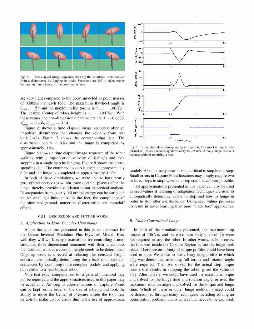
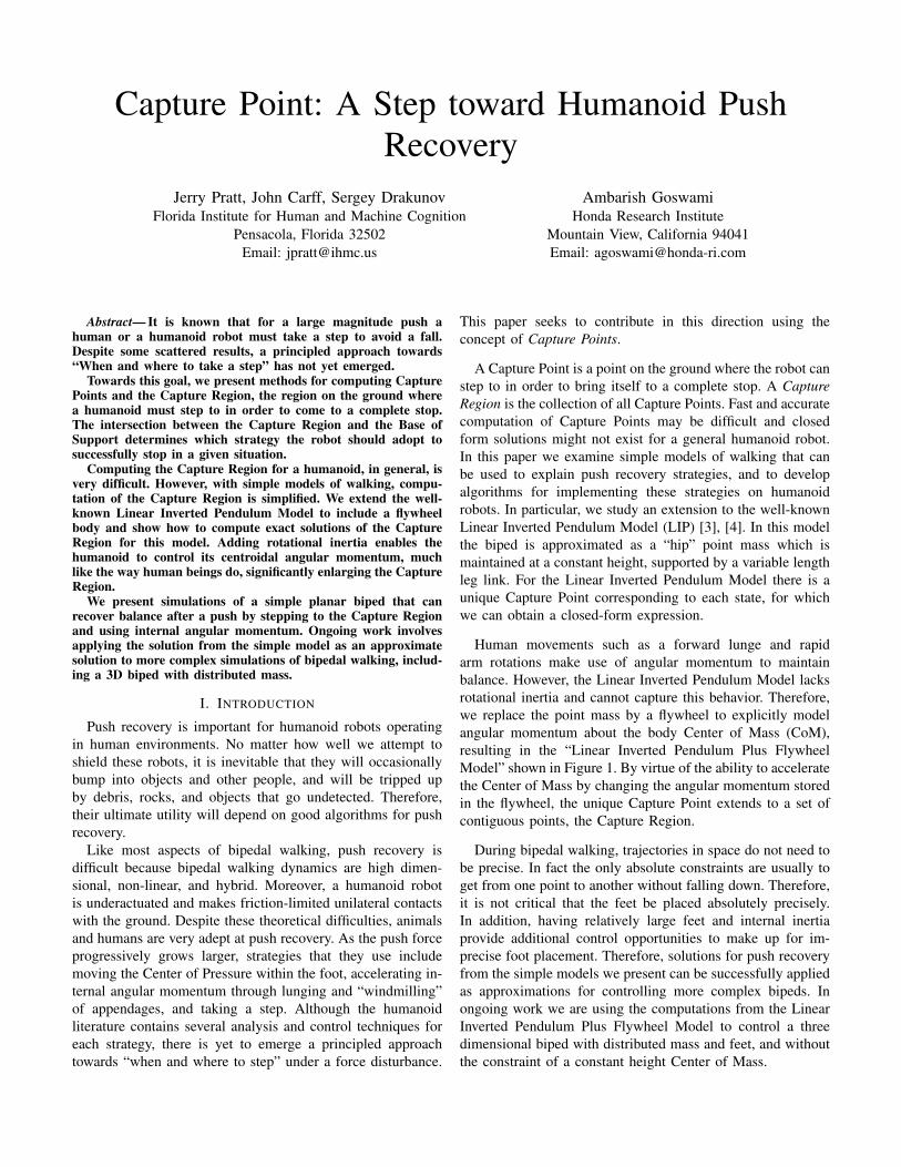
Fig. 6. Time elapsed image sequence showing the simulated robot recoverfrom a disturbance by lunging its body. Snapshots are left to right, top tobottom, and are taken at 0.1 second increments.

are very light compared to the body, modeled as point massesof 0.0025kg at each foot. The maximum flywheel angle isθmax = 3

4π and the maximum hip torque is τmax = 100Nm.The desired Center of Mass height is z0 = 0.9375m. Withthese values, the non-dimensional parameters are J ′ = 0.0558,τ ′max = 0.435, θ′max = 0.131.

Figure 6 shows a time elapsed image sequence after animpulsive disturbance that changes the velocity from restto 0.2m/s. Figure 7 shows the corresponding data. Thedisturbance occurs at 0.5s and the lunge is completed byapproximately 0.8s.

Figure 8 shows a time elapsed image sequence of the robotwalking with a top-of-stride velocity of 0.5m/s and thenstopping in a single step by lunging. Figure 9 shows the corre-sponding data. The command to stop is given at approximately3.9s and the lunge is completed at approximately 4.25s.

In both of these simulations, we were able to have nearlyzero orbital energy (to within three decimal places) after thelunge, thereby providing validation to our theoretical analysis.Discrepancies from exactly 0.0 orbital energy can be attributedto the small but finite mass in the feet, the compliance ofthe simulated ground, numerical discretization and roundoffeffects.

VIII. DISCUSSION AND FUTURE WORK

A. Application to More Complex Humanoids

All of the equations presented in this paper are exact forthe Linear Inverted Pendulum Plus Flywheel Model. Howwell they will work as approximations for controlling a non-simulated three-dimensional humanoid with distributed massthat does not walk at a constant height needs to be determined.Ongoing work is directed at relaxing the constant heightconstraint, empirically determining the effects of model dis-crepancies by examining more complex models, and applyingour results to a real bipedal robot.

Note that exact computations for a general humanoid maynot be required and the approximations used in this paper maybe acceptable. As long as approximations of Capture Pointscan be kept on the order of the size of a humanoid foot, theability to move the Center of Pressure inside the foot maybe able to make up for errors due to the use of approximate

Fig. 7. Simulation data corresponding to Figure 6. The robot is impulsivelypushed at 0.5 sec., increasing its velocity to 0.2 m/s. A body lunge recoversbalance without requiring a step.

models. Also, in many cases it is not critical to stop in one step.Small errors in Capture Point locations may simply require twoor three steps to stop, when one step could have been possible.

The approximations presented in this paper can also be usedas seed values if learning or adaptation techniques are used toautomatically determine where to step and how to lunge inorder to stop after a disturbance. Using seed values promisesto result in faster learning than pure “black box” approaches.

B. Under-Constrained Lunge

In both of the simulations presented, the maximum hiptorque of 100Nm and the maximum body pitch of 3

4π werenot required to stop the robot. In other words, in both cases,the foot was inside the Capture Region before the lunge tookplace. Therefore an infinity of torque profiles could have beenused to stop. We chose to use a bang-bang profile in whichTR2 was determined assuming full torque and rotation anglewere required. Then we solved for the actual step torqueprofile that results in stopping the robot, given the value ofTR2. Alternatively, we could have used the maximum torqueand solved for the lunge time and rotation angle, or used themaximum rotation angle and solved for the torque and lungetime. Which of these or other lunge method is used couldbe determined through many techniques, including solving anoptimization problem, and is an area that needs to be explored.

Fig. 8. Time elapsed image sequence showing the robot stop walking in asingle step by lunging its body. Snapshots are left to right, top to bottom, andare taken at 0.25 second increments.

C. Capture Region and Biped Design Considerations

Increasing the amount of available non-dimensional torque,τ ′max, or rotation angle, θ′max, increases the size of the CaptureRegion. However, if one of the values is fixed, there isdiminishing returns in increasing the other, as seen in Figures4 and 5. In addition, the maximum torque must not exceedthe value that would cause foot slipping.

Therefore, these two parameters should be designed to-gether, using Equations 38 to 41 to analyze their effect on theCapture Region. A feasible approach would be to use Equation37 to set a good maximum torque and then increase themaximum rotation angle until there are diminishing returns.Determining how maximizing the Capture Region fits in withother design criterion needs to be explored further.

ACKNOWLEDGMENTSupport for this work was provided by the Honda Research

Institute.

REFERENCES

[1] Muhammad Abdallah and Ambarish Goswami. A biomechanicallymotivated two-phase strategy for biped upright balance control. IEEEInternational Conference on Robotics and Automation (ICRA), 2005.

[2] Andreas G. Hofmann. Robust Execution of Bipedal Walking Tasks FromBiomechanical Priciples. PhD thesis, Computer Science Department,Massachusetts Institute of Technology, 2006.

[3] S. Kajita and K. Tani. Study of dynamic biped locomotion on ruggedterrain-derivation and application of the linear inverted pendulum mode.volume 2, pages 1405 – 1411. IEEE International Conference on Roboticsand Automation (ICRA), 1991.

[4] Shuuji Kajita, Fumio Kanehiro, Kenji Kaneko, Kazuhito Yokoi, andHirohisa Hirukawa. The 3d linear inverted pendulum mode: a simplemodeling for a biped walking pattern generation. pages 239 – 246. IEEEInternational Conference on Intelligent Robots and Systems (IROS), 2001.

[5] S. Kajita, F. Kanehiro, K. Kaneko, K. Fujiwara, K. Harada, K. Yokoi, andH. Hirukawa, “Resolved momentum control: Humanoid motion planningbased on the linear and angular momentum,” in IEEE/RSJ InternationalConference on Intelligent Robots and Systems, 2003, pp. 1644–1650.

[6] T. Komura, H. Leung, S. Kudoh, and J. Kuffner, “A feedback controllerfor biped humanoids that can counteract large perturbations during gait,”in IEEE International Conference on Robotics and Automation (ICRA),2005, Barcelona, Spain, pp. 2001–2007.

[7] T. Komura, A. Nagano, H. Leung, and Y. Shinagawa, “Simulatingpathological gait using the enhanced linear inverted pendulum model,”IEEE Transactions on Biomedical Engineering, vol. 52, no. 9, pp. 1502–1513, 2005, September.

Fig. 9. Simulation data corresponding to Figure 8. The robot starts walkingat a desired top-of-stride velocity of 0.5 m/s. The robot is commanded to stopshortly after taking a step at about 3.9 seconds. It does so by lunging its upperbody, without taking an additional step.

[8] A.D. Kuo and F. E. Zajac. Human standing posture: multijoint move-ment strategies based on biomechanical constraints. Progress in BrainResearch, 97:349–358, 1993.

[9] N. M. Mayer, F. Farkas, and M. Asada, “Balanced walking and rapidmovements in a biped robot by using a symmetric rotor and a brake,”in International Conference on Mechatronics and Automation, July 29-August 1, 2005, Niagara Falls, Ontario, Canada.

[10] Thomas A. McMahon and John Tyler Bonner. On Size and Life.Scientific American Library, 1983.

[11] Marko Popovic, Amy Englehart, and Hugh Herr. Angular momentumprimitives for human walking: Biomechanics and control. In Proceedingsof the IEEE/RSJ International Conference on Intelligent Robots andSystems, 2004.

[12] Marko Popovic, Ambarish Goswami, and Hugh Herr. Ground ref-erence points in legged locomotion: Definitions, biological trajectoriesand control implications. International Journal of Robotics Research,24(12):1013–1032, Dec 2005.

[13] Jerry Pratt. Exploiting Inherent Robustness and Natural Dynamics inthe Control of Bipedal Walking Robots. PhD thesis, Computer ScienceDepartment, Massachusetts Institute of Technology, 2000.

[14] Jerry Pratt and Russ Tedrake. Velocity Based Stability Margins for FastBipedal Walking. First Ruperto Carola Symposium in the InternationalScience Forum of the University of Heidelberg entitled ”Fast Motions inBiomechanics and Robots” Heidelberg Germany, September 7-9, 2005.

[15] M. J. Sidi, Spacecraft Dynamics and Control. NewYork, NY: Cam-bridge University Press, 1997.

[16] P. Tsiotras and H. Shen, “Satellite attitude control and power trackingwith energy/momentum wheels,” Jornal of Guidance, Control and Dy-namics, vol. 24, no. 1, pp. 23–34, 2001.

[17] J. Vermeulen, B. Verrelst, B. Vanderborght, D. Lefeber, and P. Guil-laume, “Trajectory planning for the walking biped.”

[18] E. R. Westervelt, J. W. Grizzle, and D. E. Koditschek. Zero dynamics ofunderactuated planar biped walkers. IFAC-2002, Barcelona, Spain, pages1–6, Jul 2002.