capture solar energy and reduce heat-island effect from

Worcester Polytechnic InstituteDigital WPI

Doctoral Dissertations (All Dissertations, All Years) Electronic Theses and Dissertations

2008-12-15

Capture Solar Energy and Reduce Heat-IslandEffect from Asphalt PavementBao-Liang ChenWorcester Polytechnic Institute

Follow this and additional works at: https://digitalcommons.wpi.edu/etd-dissertations

This dissertation is brought to you for free and open access by Digital WPI. It has been accepted for inclusion in Doctoral Dissertations (AllDissertations, All Years) by an authorized administrator of Digital WPI. For more information, please contact [email protected].

Repository CitationChen, B. (2008). Capture Solar Energy and Reduce Heat-Island Effect from Asphalt Pavement. Retrieved fromhttps://digitalcommons.wpi.edu/etd-dissertations/421

https://digitalcommons.wpi.edu?utm_source=digitalcommons.wpi.edu%2Fetd-dissertations%2F421&utm_medium=PDF&utm_campaign=PDFCoverPages

https://digitalcommons.wpi.edu/etd-dissertations?utm_source=digitalcommons.wpi.edu%2Fetd-dissertations%2F421&utm_medium=PDF&utm_campaign=PDFCoverPages

https://digitalcommons.wpi.edu/etd?utm_source=digitalcommons.wpi.edu%2Fetd-dissertations%2F421&utm_medium=PDF&utm_campaign=PDFCoverPages

https://digitalcommons.wpi.edu/etd-dissertations?utm_source=digitalcommons.wpi.edu%2Fetd-dissertations%2F421&utm_medium=PDF&utm_campaign=PDFCoverPages

https://digitalcommons.wpi.edu/etd-dissertations/421?utm_source=digitalcommons.wpi.edu%2Fetd-dissertations%2F421&utm_medium=PDF&utm_campaign=PDFCoverPages

https://digitalcommons.wpi.edu/

mailto:[email protected]

i

ABSTRACT

Asphalt pavements are made up of several layers of materials and different types

of materials are being used as base courses in these pavements. The properties of these

pavement layers are affected significantly by temperature, and all of the layers are made

up of heterogeneous mixtures of a wide variety of materials whose thermal properties are

not readily available. Therefore, laboratory experiments were carried out with samples of

pavements with different base course materials to determine temperature profiles along

the depth, and finite element analysis was used to backcalculate thermal properties of the

materials in the different layers of the different samples.

The concept of extracting heat energy from asphalt pavements was evaluated by

finite element modelling and testing small and large scale asphalt pavement samples.

Water flowing through copper tubes inserted within asphalt pavements samples were

used as heat exchangers in the experiments. The rise in temperature of water as a result of

flow through the asphalt pavement was used as the indicator of efficiency of heat capture.

The results of small scale testing show that the use of aggregates with high conductivity

can significantly enhance the efficiency of heat capture. The efficiency can also be

improved by using a reflectivity reducing and absorptivity increasing top layer over the

pavement. Tests carried out with large scale slabs show that a larger surface area results

in a higher amount of heat capture, and that the depth of heat exchanger is critical

Heat-Islands are formed as a result of construction that replaces vegetation with

absorptive surfaces (asphalt pavement). One suggested method to reduce the emitted

heat from asphalt pavement surfaces is to reduce the temperature of the surface by

flowing a suitable fluid through the pavement. Laboratory experiments were carried out

using hand-compacted hot mix asphalt samples with quartzite and metagranodiorite

aggregates. Pipes with different surface area were used to flow water through the

samples, and the processes were modeled using finite element method. The results clearly

show the feasibility of the proposed method, and indicate the beneficial effects of higher

thermal conductivity of aggregates and larger surface area of pipes.

ii

DEDICATION

This dissertation is dedicated to my parents

Mrs. Shu-Feng Chen

and

Mr. Matzuda Kazyuki

for giving me invaluable opportunities in life and for their inspiration, constant

encouragement and tremendous belief in me.

iii

ACKNOWLEDGEMENTS

I would like to express my profound gratitude to my advisor Dr. Rajib Basu

Mallick for giving me the research opportunity and his thorough guidance and

encouragement in every aspect of my research work.

I also thank my committee members Dr. Tahar El-Korchi, Dr. Mingjiang Tao, and

Dr. Shnkha Bhowmick (University of Massachuesste, Dartmouth) for their suggestions,

comments, and assistances.

I would also like to thank Mr. Mike Hulen, President of Novotech Inc.

Massachusetts Technology Collaborative Inc., and Faculty Advancement Research

(FAR) for their funding supports, and Gerard Moulzolf of American Engineering

Testing, Inc., for providing the most valuable information, and Mr. Ron Tardiff of

Aggregate Industries and Mr. Jeff Carlstrom of New Ulm Quartzite Quarries for

providing the samples.

Finally, this study would not have been possible without the laboratory and shop

help from, Mr. Don Pellegrino, Mr. Dean Daigneault, Ms. Laura Rockett, Mr. Daniel

Martel, Mr. Yanxuan Xiu, and Ms. Karen O’Sullivan of the Civil and Environmental

Engineering department at Worcester Polytechnic Institute (WPI).

iv

TABLE OF CONTENTS

CHAPTER PAGE

1. INTRODUCTION 1

1.1 Background 1

1.2 Objective of Research 2

1.3 Scope of Research 3

2. LITERATURE REVIEW 4

2.1 Prediction and validation of temperature at the surface and any

depth of asphalt and concrete pavements 4

2.2 Evaluation of effect of temperature change on material properties,

such as modulus 5

2.3 Modification of design procedures to consider the effect of

temperature change on pavement material properties 5

2.4 Investigate the feasibility of using heat from solar heated asphalt

pavements 11

2.5 Evaluation of Heat-Island Effect on reducing pavement

temperature 11

2.6 Discussion 12

3. HEAT TRANSFER 15

3.1 Analytical Approach 15

3.2 Energy Balance of Asphalt Pavement 22

3.3 Finite Element Analysis Approach 26

4. DETERMINE THERMAL PROPERTIES OF EXISTING

ASPHAPLT PAVEMENT 30

4.1 Introduction 30

4.2 Objective 30

4.3 Methodology 30

4.4 Laboratory Parameters Measurement 34

4.5 Experiment Results 39

4.6 Statistical Approach of Determining Temperature at Specific

Location 46

v

CHAPTER PAGE

4.7 Finite Element Analysis/Modeling 48

4.8 Discussion 56

5. SMALL SCALE ASPHALT PAVEMENT TESTING 59

5.1 Introduction 59

5.2 Objective 59

5.3 Methodology 59


5.5 Robustness Test 80


5.7 Discussion 87

6. HAND-COMPACTED ASPHALT PAVEMENT TESTING 88

6.1 Introduction 88

6.2 Objective 88

6.3 Methodology 88



6.6 Discussion 96

7. DETERMINE EFFECTIVE PIPE LENGTH AND SPACING 97

8.1 Introduction 97

6.2 Objective 97

6.3 Methodology 97



6.6 Discussion 107

8. REDUCE URBAN HEAT-ISLAND EFFECT 108

7.1 Introduction 108

7.2 Objective 108

7.3 Methodology 108


7.5 Discussion 123

vi

CHAPTER PAGE

9. LARGE SCALE ASPHALT PAVEMENT TESTING 124

9.1 Introduction 124

9.2 Objective 127

9.3 Methodology 127



9.6 Discussion 150

10. CONCLUSION 151

11. FUTURE STUDY RECOMMENDATION 153

11.1 What is the effect of water outlet temperature by using

different pipe materials? 153

11.2 How to increase the water temperature to meet the minimum

temperature requirement of turbine to generate electric? 153

11.3 How much pavement life can be extended by using asphalt

pavement as solar collector? 154

12. REFERENCE 156

APPENDIX

A SIX HIGHTWAY PAVEMENT THERMOCOUPLE 160

B DETERMINE THMERAL PROPERTIES OF R, P401, M,

AND FR SAMPLES 163

C EXPERIMENT SETUP FOR EACH SCENARIO 173

D DETERMINE THERMAL PROPERTIES OF QUARTZITE ,

LIMESTONE, AND METAGRANODIORTE (SMALL SCALE) 177

E LARGE SCALE PAVEMENT PREPARATION 183

F SKETCH AND DIMENSION OF HAND-COMPACTED SAMPLES 187

G DETERMINE THERMAL PROPERTIES OF METAGRANDODIORITE

AND QUARTZITE (HAND-COMPACTED) 190

vii

LIST OF TABLES

TABLE PAGE

4-1 Types of pavements considered 32

4-2 Measured heat parameters 37

4-3 Measured emissivity values 38

4-4 G Sample - Highway-HMA layers over HMA base with different NMAS 39

4-5 S Sample -HMA layers over PMRAP base 40

4-6 M Sample- HMA layers over Foamed Asphalt base 41

4-7 R Sample- HMA layers over cement treated base 42

4-8 P401 Sample- HMA layers of same NMAS 43

4-9 FR Sample- HMA layers of different types two lifts 44

4-10 Equation from statistical analysis 47

4-11 Back-calculated thermal conductivity and heat capacity values 57

5-1 Quartzite and Limestone mix temperature difference 63

5-2 Quartzite mix with and without placement of tinted glass temperature

difference 63

5-3 100% Quartzite with iced water (3mL/min) temperature difference 64

5-4 100% Quartzite mix with trapped iced water inside of cooper pipe

temperature difference 64

5-5 Complied of 5 quartzite samples with 0.01905m (¾”) copper pipe


5-6 100% Quartzite mix temperature difference 67

5-7 100% Metagranodiorite mix temperature difference 67

5-8 100% RAP mix temperature difference 67

5-9 Quartzite with 22% copper mix temperature difference 70

5-10 Quartzite with 30% aluminum mix temperature difference 70

5-11 Quartzite with 50% RAP mix temperature difference 72

5-12 Quartzite with 75% RAP mix temperature difference 72

5-13 67% quartzite with 33% limestone mix temperature difference 72

5-14 Tinted glass on the surface of quartzite with 22% copper mix


viii

TABLE PAGE

5-15 Acrylic paint on the surface of quartzite with 22% copper mix temperature

difference 75

5-16 Tinted glass on the surface of quartzite with 30% aluminum mix temperature

difference 76

5-17 Chipped glass with asphalt mix on the quartzite with 30% aluminum mix


5-18 Repetitive test of 67% quartzite and 33% limestone mix 80

5-19 Thermal properties of quartzite and limestone sample mix (Appendix D) 81

5-20 Thermal properties of quartzite and metagranodiorite mix (Appendix D) 86

6-1 Description of compacted samples (Appendix E) 89

6-2 Temperature difference at time= 60 minutes (Lab Data); water flowing at

10 ml/minute 92

6-3 Temperature difference at time= 180 minutes (Lab Data) 93

6-4 Quartzite mix back-calculated thermal properties 94

6-5 Metagranodiorite mix back-calculated thermal properties 94

6-6 Laboratory and FE temperature difference at time = 60 minutes

comparison 95

6-7 Laboratory and FE temperature difference at time = 180 minutes

comparison 95

7-1 The typical Nusselt number for fully developed flow 98

7-2 Required pipe length at wall temperature= 50 °C 98

7-3 Average water temperature difference at time= 60 minutes 101

7-4 Average water temperature difference at time= 180 minutes 102

7-5 Water temperature comparison 107

8-1 Average Reduction in surface temperature due to flowing water 118

9-1 Metagranodiorite slab water temperature (all pipe open) 132

9-2 Quartzite slab water temperature (all pipe open) 133

9-3 Quartzite slab temperature profile with 1L/min (1 pipe) 134



ix

TABLE PAGE


9-7 Quartzite slab temperature profile with 1L/min (2 pipes open) 138

9-8 Thermal conductivity and heat capacity of two slab mix 142

9-9 Quartzite slab 1L/min (35mins) 145




x

LIST OF FIGURES

FIGURE PAGE

2-1 Energy balance on asphalt surface 6

3-1 Energy balance on the surface of a grey body 22

4-1 Six existing highway samples 33

4-2 Laboratory testing setup 34

4-3 Location of thermocouples in different samples 35

4-4 Halogen lamp heat radiation measurement 36

4-5 Laboratory testing setup with fan and anemometer 37

4-6 G Sample temperature distribution (7-days cycle) 39

4-7 S Sample temperature distribution (7-days cycle) 40

4-8 M Sample temperature distribution (7-days cycle) 41

4-9 R Sample temperature distribution (7-days cycle) 42

4-10 P401 Sample temperature distribution (7-days cycle) 43

4-11 FR Sample temperature distribution (7-days cycle) 44

4-12 6 Samples temperature distribution at end of 7th heating cycle 45

4-13 Mesh generated from COMSOL 49

4-14 COMSOL simulation result 49

4-15 G sample temperature at T2

(finite element predicted vs. laboratory results) 51









4-20 S sample temperature at T2


xi

FIGURE PAGE









5-1 Small scale testing (Scenario I) temperature difference ΔT 63

5-2 Small scale testing (Scenario II) temperature difference ΔT 65

5-3 Small scale testing (Scenario II) power generated 65

5-4 Typical asphalt sample with thermocouples 66

5-5 Small scale testing (Scenario III) temperature vs. flow rate 68

5-6 Small scale testing (Scenario III) temperature difference ΔT 69

5-7 Small scale testing (Scenario III) power generated 69

5-8 Small scale testing (Scenario VI) effect of copper powder 71

5-9 Small scale testing (Scenario VI) effect of aluminum powder 71

5-10 Small scale testing (Scenario VI) temperature vs. flow rate 73

5-11 Small scale testing (Scenario VI) temperature difference ΔT 74

5-12 Small scale testing (Scenario VI) power generated 74

5-13 Small scale testing (Scenario VI) temperature vs. flow rate 76

5-14 Small scale testing (Scenario V) temperature difference ΔT 77

5-15 Small scale testing (Scenario V) power generated 77

5-16 Effective of Acrylic Paint 78

5-17 Small scale testing temperature difference ΔT 79

5-18 5-days repetitive test of 67% quartzite and 33% limestone mix 80

5-19 Steady-state finite element model 82

5-20 Transient finite element model 82

5-21 Water temperature distribution along the length of copper pipe (Quartzite) 84

xii

FIGURE PAGE

5-22 Water temperature distribution along the length of copper pipe

(Metagranodiorite) 84

5-23 Water temperature distribution along the depth of copper pipe (Quartzite) 85

5-24 Water temperature distribution along the depth of copper pipe

(Metagranodiorite) 85

5-25 Quartzite mix temperature profile 86

6-1 Copper pipe with 6 rings 90

6-2 Placed thermocouples on top layer 90

6-3 Drilled vs. compacted sample temperature distribution 91

6-4 Average water temperature difference at time = 60 minutes 92


7-1 Effective pipe diameter, length, and flow rate chart 99

7-2 Serpentine pipe being placed and compacted 100



7-5 Temperature variation between two pipes 103

7-6 Finite element model for temeprature variation between various

pipe spacing 104

7-7 Straight pipe 0.1524m (6”) (temperature distribution) 105

7-8 Serpentine pipe 0.3556m (14”) (temperature distribution) 105

7-9 Serpentine pipe 0.7112m (28”) (temperature distribution) 106

8-1 Samples with three thermocouples 110

8-2 Quartzite and metagranodiorite mixes for 8 hour heating and 8 hour

no heating data for surface temperature (T2 thermocouple) 111

8-3 Heating with water flow data for surface temperature

(T2 thermocouple) for quartzite and metagranodiorite mixes 112

8-4 Schematic of thermocouple locations on the surface of asphalt sample 113

8-5 Thermocouple locations on the surface of asphalt sample 113

8-6 Plot of time versus temperature (T1) 114


xiii

FIGURE PAGE






8-13 Serpentine pipe in a sample (during compaction) 119








9-1 Schematics of slab with thermocouple, copper pipes, and water flow

direction 125

9-2 Dimension of slab and copper frame 125

9-3 Metagranodiorite mix slab thermocouple location 126

9-4 Quartzite mix slab thermocouple location 126

9-5 Two slabs tests under the real environmental conditions 128

9-6 Metagranodiorite mix slab temperature profile 129

9-7 Quartzite mix slab temperature profile 130

9-8 Metagranodiorite slab thermocouple locations 131

9-9 Water temperature measured at 3ft pipe outlet for both slabs 132

9-10 Water temperature measured at 6ft pipe outlet for both slabs 133

9-11 Quartzite mix slab temperature profile (1L/min) 134




9-15 Quartzite mix slab temperature profile (1L/min at 2 3ft pipes) 138

9-16 Quartzite slab temperature profile (1 pipe with 1L/min) 139

xiv

FIGURE PAGE

9-17 Quartzite slab temperature profile (2 pipe s with 1L/min) 139

9-18 Solar Radiation 140

9-19 Finite element mesh model 141

9-20 Finite element model of heating period 141

9-21 Quartzite slab temperature profile of heat-up period 142

9-22 Finite element model with various water flow rates 143

9-23 Finite element mesh model 143

9-24 Water temperature distribution along the length of copper pipe 144

9-25 Water temperature distribution along the depth of copper pipe 144

9-26 Quartzite slab temperature profile 1L/min

(laboratory vs. finite element analysis) 145



9-28 Quartzite slab temperature profile 3 L/min




9-30 Quartzite slab water temperature at various water flow rate


11-1 Extended service life of pavement by reducing pavement temperature 155

A-1 G Sample - Highway-HMA layers over HMA base with different NMAS 160

A-2 S Sample -HMA layers over PMRAP base 160

A-3 M Sample- HMA layers over Foamed Asphalt base 161

A-4 R Sample- HMA layers over cement treated base 161

A-5 P401 Sample- HMA layers of same NMAS 162

A-6 FR Sample- HMA layers of different types two lifts 162

B-1 R sample temperature at T2




xv

FIGURE PAGE







B-6 P401 sample temperature at T2










B-11 M sample temperature at T2










B-16 FR sample temperature at T2




xvi

FIGURE PAGE







C-1 Steady-state setup 173

C-2 Steady-state setup with halogen lamp on 173

C-3 Complied 5 asphalt pavement testing 174

C-4 Complied 5 asphalt pavements testing without halogen lamp on 174

C-5 Transient testing setup 175

C-6 Glass chips-Asphalt mix placed on top of asphalt sample 175

C-7 Tinted glass placed on top of asphalt sample 176

D-1 Quartzite sample temperature at T2








D-5 Limestone sample temperature at T3






D-8 Metagranodiorite sample temperature at T2


xvii

FIGURE PAGE







E-1 100% Metagranodiorite mix 183

E-2 100% Quartzite mix 183

E-3 50% Quartzite on the top and 50% Metagranodiorite on the bottom 184

E-4 35% Metagranodiorite on the top, 30% quartzite in the center layer,

and 35% Metagranodiorite on the bottom 184

E-5 100% Metagranodiorite mix with Portland cement placed around

copper pipe 185

E-6 100% Quartzite mix with a copper pipe consists 6 rings 185

E-7 100% Quartzite mix with a rough surface copper pipe 186

F-1 Metagranodiorite sample temperature at T2






F-4 Quartzite sample temperature at T4






G-1 Cart with thermocouple at the bottom 190

G-2 Lay down of mix 190

G-3 Compaction 191

xviii

FIGURE PAGE

G-4 Fixing thermocouples 191

G-5 Copper pipe frame 192

G-6 Close-up of slab showing copper tube and thermocouples at

different depths 192

G-7 Completed slab ready for testing 193

1

CHAPTER 1

INTRODUCTION

1.1 Background

Asphalt pavements consist 95% of major roadway in the United States, and their

performance and longevity are greatly affected by the change of temperature. Research

has shown that there is a temperature distribution inside asphalt pavements, in the

different layers, which are in many cases made up of different materials. The temperature

distribution along the depth actually depends on the properties of these different layers –

the temperature at any layer is affected significantly by the thermal properties of the

layers above and below it. Thus, the temperature distribution in a full depth asphalt

pavement will be different from, for example, an asphalt pavement with an aggregate

base, even though the asphalt mixtures/materials in the two pavements are the same. This

is of practical significance considering the wide variety of materials that are currently

being used as base material in both highway and airfield pavements.

The sun provides a cheap and abundant source of clean and renewable energy.

Solar cells have been used to capture this energy and generate electricity. A useful form

of “cell” could be asphalt pavements, which get heated up by solar radiation. The “road”

energy solar cell concept takes advantage of a massive acreage of installed parking lots,

tarmacs and roadways.

The heat retained in the asphalt mixture can continue to produce energy after

nightfall when traditional solar cells do not function. The idea of capturing energy from

pavement not only turns areas such as parking lots into an energy source, but also could

cool the asphalt pavements, thus reducing the Urban Heat-Island Effect.

The significance of this concept lies in the fact that the massive installed base of

parking lots and roadways creates a low cost solar collector an order of magnitude more

productive than traditional solar cells. The significantly high surface area can offset the

expected lower efficiency (compared to traditional solar cells) by several orders of

magnitude, and hence result in significantly lower cost per unit of power produced.

2

The system uses an existing lot, so does not require purchase or lease of new real

estate (as would be needed for a solar “farm” installation). The system has no visible

signature — that is, the parking lot looks the same. This compares well against rooftop

silicon panels that are often bulky and unattractive. The fact that roads and parking lots

are resurfaced on a 10-12 year cycle could be a good selling point for the road energy

system - any time the pavement is replaced, the energy system can be installed.

The captured energy from heated asphalt pavements can be used for relatively

simple applications, such as heating of water, to sophisticated applications, such as

generating electricity through thermoelectric generators. In addition, the benefit of lower

asphalt pavement temperature can also reduce Urban Heat-Island Effect to improve the

human comfort level in the major cities.

1.2 Objective of Research

The objectives of this research were to:

1. Investigate the temperature distribution along the depth of asphalt pavements with

laboratory experiments.

2. Build statistical models to predict the temperature in different base layers.

3. Model the temperature distribution, using principles of heat transfer in different

pavements and determine appropriate values of thermal properties of the different layers

4. Investigate the feasibility of enhancing the amount and rate of flow of heat energy

from heated asphalt pavements by using appropriate primary construction materials,

additives, and modification of top layer of the pavement.

5. Use theoretical approach to develop a relationship among flow rate, pipe diameter, and

pipe length.

6. Investigate different pipe geometries to increase heat transfer from asphalt pavement to

water.

7. Investigate the possibility of reducing Urban Heat-Island Effect.

3

1.3 Scope of Research

The scope of this research consists of

1. Performing a series of iterature review on prediction of asphalt pavement

temperature, extraction of heat energy from asphalt pavement, and

reducing Urbran Heat-Island Effect by lowering asphalt pavement

temperature.

2. Determining thermal properties of the existing highway and airport

samples with different materials layers.

3. Developing the statistical models to predict the temperature relationship of

1-inch above surface, surface, and 1-inch below surface for six existing

highway and airport samples.

4. Evaluating the heat energy tranfer of different small scale asphalt mix

samples with high conductive fillers, aggregates, and modified surface

conditions.

5. Evaluating the heat energy tranfer ability by using different asphalt mix

layers and copper pipe layouts, and increase contact of asphalt mix and

copper pipe in hand-compacted asphalt samples.

6. Determining the effective copper pipe length, spacing, and water flow rate

for asphalt solar collector systems by using analytical apporach.

7. Evaluating the feasibility of reducing Urban Heat-Island Effect by using

higher thermal conductivity aggregate and different pipe layouts.

8. Evaluating the feasibility of heat energy transfer by performing field tests

with two large scale asphalt pavements.

9. Analyzing and evaluating the experiement data with backcalculated

thermal properties from finite element analysis, and deternine the effect of

thermal conductivity, asphalt composition, pipe layout, and water flow

rate.

4

CHAPTER 2

LITERATURE REVIEW

Studies have been carried out on different aspects of temperature change and its

effect on pavements. These studies can be broadly classified into five types: 1. Prediction

and validation of temperature at the surface and any depth of asphalt and concrete

pavements; 2. Evaluation of effect of temperature change on material properties, such as

modulus; 3. Modification of design procedures to consider the effect of temperature

change on pavement material properties; 4. Investigation of the feasibility of using heat

from solar heated asphalt pavements. 5. Evaluation of Urban Heat-Island Effect on

reducing pavement temperature.

Since the focus of this study is on topics 1, 4, and 5, the literature review will be

restricted to that pertinent topics only.

2.1 Prediction and validation of temperature at the surface and any depth of

asphalt and concrete pavements

The earliest published work is that by Southgate (1) who presented a method for

predicting temperatures in asphalt pavement layers, as a function of depth, time of the

day, and the 5-day mean air temperature.

Hermansson (2) presented a procedure based on finite difference procedure to

determine pavement temperatures. This procedure estimates pavement temperatures at

different depths using formulas that consider convection, short and long-wave radiation,

and a finite difference approximation for the calculation of heat transfer into the

pavement through the subsurface layers. For calculating heat transfer, the pavement is

divided into cells, each of which is assigned a different value for temperature, porosity

and degree of saturation. The proposed model can, according to comparisons with field

experiments, calculate temperatures of pavement at different depths during summer days

using hourly solar radiation, air temperature and wind velocity as weather input. The

model proved to be accurate, having errors around 2°C for different parameters.

5

2.2 Evaluation of effect of temperature change on material properties, such as

modulus

In their study on asphalt pavement layer temperature prediction, Park, Dong-

Yeob, et al. (3) collected a large amount of temperate data and deflection profiles from

various sites in Michigan to investigate how temperature affects the in-place strength of

asphalt mixes. The goal was to develop a model that could cover all seasons and various

climatic and geographic regions. Previous methods have utilized temperature data from 5

days and did not take into consideration temperature gradients due to heating and cooling

cycles. Results yielded the following temperature model, which was validated by using

data from other sites, proving the model is applicable to various regions (z = pavement

depth, t = time).

)0967.53252.6sin(

)00196.00432.03451.0( 32

+−

×+−−+=

tzzzTT sufs

A correction factor was calculated for the asphalt mix layer modulus to correct for

the difference between predicted and actual temperatures at the mid-depth of the

pavement. The measured and predicted temperature values were consistent, meaning that

the temperature prediction model and correction procedures were valid. Using prediction

of rutting, the effects of error between the calculated and measured temperatures were

determined to be very minimal. The newly formed temperature model accounted for

temperature gradients, which varied depending on the time of day due to the heating and

cooling cycle.

2.3 Modification of design procedures to consider the effect of temperature

change on pavement material properties

Yavuzturk et al (4) presented the results of a study on the use of finite difference

method to predict pavement temperature. They mention that thermal conditions which

pavements are exposed to greatly affect the performance and longevity of the pavement,

and current models to predict temperature gradient could be inaccurate because they fail

to account for the thermal history and thermal interaction between asphalt of varying

grades and contents. This paper proposes a new method to predict pavement temperatures

at various depths and horizontal locations using a transient, two-dimensional finite-

6

difference model of a pavement section. Figure 2-1 shows the primary modes of heat

transfer that have been considered in a pavement. Sensitivity analyses were conducted in

order to assess the dependency of the predicted temperature on the thermal properties.

The highest discrepancy occurred at the pavement’s surface because of more heat

dissipation as it is exposed to open air. The longer the asphalt section, the more heat is

transferred from it because the wind over the surface in longer segments is more likely to

assume a turbulent fluid flow regime, allowing for lower temperatures because of

increased cooling from heat transfer. Temperature difference ranges were found to be

much larger in the summer than in the winter. Temperature predictions using the

proposed model were most sensitive to (in decreasing order) variations in absorptivity,

volumetric specific heat capacity, emissivity, and thermal conductivity of the mix. They

conclude that further work could be done on bridge segments as the bridge deck does not

allow for an adiabatic boundary causing a cooling convection from underneath.

Figure 2-1 Energy balance on asphalt surface

7

Currently, the most widely cited temperature prediction equations for asphalt

pavements are those based on the work by Solaimanian and Kennedy (5) and from SHRP

and LTPP studies (6, 7). Solaimanian and Kennedy developed a method to be used

mainly for Strategic Highway Research Program binder and mixture specifications to

calculate the maximum pavement temperature profile. The method was based on energy

balance and temperature equilibrium at the pavement surface by using the measured data

of hourly solar radiation, wind velocity, and emissivity from various test locations. The

proposed equation was able to predict the maximum pavement temperature at specific

location within 3 °C error, which was within the reasonable limit- considering various

environmental factors and measurement uncertainty.

SHRP high temperature model equations for Superpave Mixes are:

4.242289.000618.0 2 ++−= latlatTT airsurf

( ) )0004.0007.0063.01( 32)(, dddTT surfindepth −+−=

78.17)9545.0)(4.422289.000618.0( 220 −++−= latlatTT airmm

LTTP high temperature model equations are:

5.02

102

)61.09(

)25(log14.150025.078.032.54

air

airpav

Sz

HlatTT

+

++−−+=

Where Tpav is high asphalt pavement temperature below surface (°C); Tair is high air

temperature (°C); lat is latitude of the section (degrees); H is depth to surface (mm); Sair is

standard deviation of the high 7-day mean air temperature (°C); z is Standard normal dist.

table, z is 2.055 for 98% reliability Statistics: R2

SHRP low temperature model equations are:

= 76%, N = 309, SEE = 3.0.

( )2

)(, 000063.051.0 ddTT surfmmd −+=

50% reliability: airpav SzdTT ×−= )(

8

Where Tpav is low asphalt pavement temperature with reliability (°C); T(d) is Low asphalt

pavement temperature at calculated depth (°C); Sair

LTTP low temperature model equations are:

is Standard deviation of the low air

temperature (°C); z is standard normal dist. table, z = 2.055 for 98% reliability.

5.02

102

)52.04.4(

)25(log26.6004.072.056.1

air

airpav

Sz

HlatTT

+

−++−+−=

Where Tpav is low asphalt pavement temperature below surface (°C), Tair is low air

temperature (°C), lat is latitude of the section (degrees), H is depth below surface (mm),

Sair

The most recent validation of these equations has been from the NCAT test track

(8). The study concluded that:

is Standard deviation of the mean low air temperature (°C), z is standard normal dist.

table, z = 2.055 for 98%, and z = 0.0 for 50% Statistics: Rz= 96%, N= 411, SEE = 2.1.

1. At 20, 35, 50 and 100 mm below the pavement surface, SHRP high temperature model

closely predicted actual temperatures in 2001 and slightly under-predicted temperatures

in 2002.

2. LTTP high temperature closely predicted temperatures in 2001 but underestimated in

2002 as much as 5.5°C (10°F).

3. Both low temperature models over predicted temperatures at both 50 and 98%

reliability.

4. Mix type (open/dense graded, for example) on the surface has an effect on the

temperature on underlying layers.

5. The thicker the surface, the cooler the underlying layers.

6. Pavement temperatures varied by as much 28°C (50°F) during a 24-hour period.

Diefenderfer et. al. (9) developed an equation on the basis of work conducted on

the Virginia Smart Road project. The following model was developed to predict

temperature at a depth (maximum depth below the surface = 0.188m):

9

dmp dPcYbTaT +++=

Where Tp is predicted pavement temperature (°C), a is intercept coefficient, b is ambient

temperature coefficient, Tm is measured ambient temperature (°C), c is day of year

coefficient, Y is day of year (1 to 183), d is depth coefficient; and Pd

The day of year coefficient was used in the early stages of the model instead of

solar radiation and increased linearly from January 1 to July 2, then decreased linearly

from July 3 to December 31.

is depth within the

pavement (m).

Initial model to predict maximum pavement temperatures

(RMSE = 3.54, adjusted R2

dps PYTT 7975.271061.06356.02935.3 maxmax −++=

= 91.36%) is:

Initial model to predict minimum pavement temperature

(RMSE = 2.79, R2

dps PYTT 2385.708611.065041.06472.1 minmin −++=

= 91.41%) is:

Calculated solar radiation is introduced to predict pavement temperatures at all

locations where latitude is known. (The paper describes the steps to calculate solar

radiation at any location on any day. From that new temperature models are derived)

The equation to predict the maximum pavement temperature using solar radiation is

(RSME = 5.76, R2

dsp PRTT 8739.27106736.56861.078752.2 4maxmax −××++= −

= 77.07%):

Where Tpsmax is predicted pavement temperature (°C), Tmax is maximum daily ambient

temperature (°C), Rs= calculated daily solar radiation (kJ/m2-day); and Pd

The equation to predict minimum pavement temperature using solar radiation is (RSME

= 4.28, R

is depth from

the surface (m).

2

dsps PRTT 2043.710764.36754.02097.1 4minmin +××++−= −

= 79.79%):

10

Data from two randomly selected LTTP-SMP sites was used to validate the

equations above. Using the data, new models were formulated which incorporated the

day of year and latitude.

While most of the studies have been conducted on the basis of field data, a series

of laboratory studies have been conducted by Mrawira and his colleagues at the

University of New Brunswick. In several papers they describe the use of a laboratory set

up to observe temperatures at different depths of HMA samples, and another equipment

to determine thermal/heat properties of HMA.

In their 2002 TRB paper (10), the authors describe an approach in which thermal

diffusivity and corresponding thermo-physical properties are measured. These properties

were found to be affected by density, saturation and temperature. Using the estimated

thermal conductivities, the authors predicted the transient temperature conditions in an

asphalt pavement under changing environmental conditions. They used energy balance

equation and Fourier heat transfer equation. They show from their results that the asphalt

pavement goes through daily temperature cycles, and the relative amplitude of such

cycles decrease with an increase in depth.

Subsequently, in their 2004 TRB paper (11) Luca and Mrawira describe a

laboratory device to observe temperature changes inside a 150 mm diameter asphalt mix

sample when subjected to heat from a halogen lamp. Varying wind speeds were created

with the help of a fan positioned close to the sample. For the configuration, the authors

predicted the time-temperature data with a finite difference approach. And the predicted

and actual data were found to be in good agreement. The authors conclude that thermal

radiation is the most critical factor affecting the rate of change in temperature, which was

higher at depths closer to the surface.

In their 2005 paper (12), Luca and Mrawira point out the importance of getting

reliable thermo-physical data for the proper implementation of transient temperature

models, and that the existing ASTM C177-85 is not suitable for testing HMA. They

present a new method for determination of thermal properties of HMA. They used the

new device to determine thermal conductivity in steady state and thermal diffusivity in

transient state. They compared their obtained values with those found in the literature.

11

Based on their studies they conclude that there is no correlation between thermal

properties and resilient modulus and Marshal stability

2.4 Investigate the feasibility of using heat from solar heated asphalt pavements

As summarized by Bijsterveld et al (13) there are three potential ways of utilizing

the heat from pavements. The heat can either be used to provide heating energy to

buildings, or used to melt snow on the pavement during winter and keep its temperature

at a higher than natural level, or can be extracted away from the pavement during the

summer time to reduce the potential of permanent deformation (or rutting). In their paper,

Bijsterveld et al describes a finite element modeling study to investigate the effects of

providing a heat exchanger system inside the pavement on the temperature distribution,

as well as stress, strains inside the pavement. They conclude on the basis of results

obtained from the models that locating the heat exchanger tubes at shallow depths would

allow extraction of more energy but would result in higher stresses in the pavement,

which could reduce the durability of the pavement. They mention that there is a need to

determine the effect of different materials on the thermal and structural properties of the

pavement. Hasebe et al (14) has reported a study on the use of energy from heated

pavements to produce electricity, and use the heat flux away from the pavement to lower

high pavement temperatures during summer. Their study involved conducting

experiments and modeling to evaluate the effect of the flow rate and temperature of the

heat exchanger. They confirmed the significant effect of the temperature of the heat

exchanger fluid and the resistance of the thermoelectric modules on the peak power

output.

2.5 Evaluation of Urban Heat-Island Effect on reducing pavement temperature

Heat-islands are formed as vegetation is replaced by asphalt and concrete for

roads, buildings, and other structures, which absorb - rather than reflect - the sun's heat,

causing surface temperatures and overall ambient temperatures to rise (15). The heat

from asphalt pavements is a major contributor to the rise in temperature in areas with

asphalt pavements, resulting in what is known as the Urban Heat-Island Effect (16). The

Urban Heat-Island effect is created by the high absorptivity of the pavement surface

12

which subsequently leads to an elevated surface temperature and therefore higher

emission from the pavement (17).

In their recent paper Gui et al (18) have presented a mathematical model to

calculate the pavement near-surface temperatures using hourly measured solar radiation,

air temperature, dew-point temperature, and wind velocity data. Their objective was to

determine optimum combination of material properties and/or paving practices to lower

air temperature rise caused by paving materials in urban areas. They point out that

reflectivity and emissivity have the highest positive effects on pavement maximum and

minimum temperatures, respectively, while increasing the thermal conductivity,

diffusivity, and volumetric heat capacity is effective in lowering maximum temperatures.

Various techniques have been proposed to lower the heat island effect. For

asphalt pavements, one prominent method proposed is to use specialized reflective

coating so that the albedo is significantly increased (19). This approach has allowed

significant lowering of surface temperature. Increased surface reflectivity may increase

visibility problems during the daytime. Also, there is a possibility that the reflected light

may be absorbed by other surfaces.

2.6 Discussion

1. Studies have been conducted both in the laboratory and with field data for

predicting pavement temperature at different depths.

2. Studies have primarily focused on steady state conditions, although some work on

transient conditions has been conducted.

3. The main drawback in conducting transient condition analysis is the lack of

appropriate thermal properties of HMA.

4. A laboratory set up has been proposed for conducting tests to observe

temperatures at different depths of a pavement, and relate those temperatures to

surface temperature.

5. A laboratory set up has been developed to estimate thermal properties of HMA in

the laboratory – this procedure is proposed as a better method compared to the

current ASTM standard test procedure.

13

6. Based on limited studies it has been shown that physical properties such as

saturation, density and temperature affect thermal properties. However, no

correlation has been observed between thermal properties and mechanical

properties such as stability and modulus.

7. A significant amount of work has been conducted to develop models to predict

temperatures at different depths of asphalt pavements.

8. A number of significant factors affecting heat flow in asphalt pavements have

been identified.

9. The feasibility of using heat from solar heated asphalt pavements has been

investigated.

10. The studies have been showed that the Urban Heat-Island Effect is created by

high absorptivity of the pavement surface and asphalt pavement is a major

contributor.

Note that so far the most of the studies have been conducted assuming full depth

HMA pavements, and temperatures at different depths of HMA have been predicted.

However, in practice, in many cases, the pavement structure consists of layers of different

materials, and the effect of such materials on the temperature distribution within the

pavement has not been studied. The feasibility of using heat from heated asphalt

pavements has been investigated, however, how to improve the performance of heat

exchanger (asphalt pavement) such as effective of pipe location, length and spacing,

water flow rate, geometry of pipe layout, enhancing thermal conductivity materials, and

how to reduce the Urban Heat Island Effect by utilizing heat exchanger design have not

been studied

This study was carried out in an attempt to answer these questions:

1. What is the effect of using different materials in different layers on the

temperature distribution inside the pavement structure?

2. Is the effect similar to or different from the case of a full depth asphalt pavement?

3. How to predict the temperature in the base layers, specifically when those layers

are made up of different materials?

14

4. What is the effect of heat transfer capability of asphalt mix when the overall

thermal conductivity is increased?

5. What is the effective design of heat exchanger to generate higher ΔT?

6. What is the effect of higher thermal conductivity of aggregates on reducing Urban

Heat-Island Effect?

15

CHAPTER 3

HEAT TEANSFER

3.1 Analytical Approach

Heat transfer is when the energy transfer from one substance to another substance

without work done and only result in temperature difference. Heat transfer can be

classified into three categories, conduction, convection, and radiation (20).

Conduction

The heat transfer by conduction is the energy transfer through a substance, a solid

or a fluid as result of the presence of a temperature gradient within the substance. This

process is also referred to as the diffusion of energy or heat. Fourier’s law is used to

calculate the conduction or diffusion energy in a substance; and it states that the heat flux

is directly proportional to the magnitude of the component of the temperature gradient in

the direction of the flux.

zTkq

yTkq

xTkq zyx ∂

∂−=

∂∂

−=∂∂

−=."

."

." .,,

Another way to express the speed of heat transfer propagating from one point to

another is thermal diffusivity, which is the ratio of thermal conductivity to volumetric

heat capacity.

pckρ

α =

Where k is thermal conductivity, ρ is density, and Cp

It measures the ability of a material to conduct thermal energy relative to its

ability to store thermal energy. Materials of large α will response quickly to changes in

their thermal environment, while materials of small α will response slowly, taking longer

to reach a new equilibrium condition.

is the specific heat of the material.

16

The thermal conductivity (k) is a thermophysical property of the substance

through which the heat flows and has the units of W/m·K. It is directly related to the

microscopic mechanism involved in the transfer of heat within the matter.

Heat capacity, also known simply as specific heat (C) is the measure of the heat

energy required to raise the temperature of a given amount of a substance by one degree

Kelvin (or Celsius). The term specific in the physical sciences often refers to quantities

divided by a specified reference quantity or amount, and in the case of specific heat

capacity, the term usually means that the heat capacity is mass-specific, or "per unit of

mass."

Convection

The heat transfer by convection is the energy transfer between a fluid and a solid

surface. There are two different types of heat convection, the first type is when the

diffusion or conduction of energy through the air or fluid because of the presence of a

temperature gradient within the fluid or called natural convection.

The second type is the transfer of the energy within the fluid due to the movement

of the fluid from one thermal environment, temperature field, to another or called forced

convection.

The magnitude (Q) of the rate of energy transfer by convection can be expressed

by Newton’s law of cooling:

ThAQ ∆=.

Or

Tqh∆

=

."

Where A is the surface area of the body which is in contact with the fluid, ΔT is the

appropriate temperature difference, q” is the heat flux, and h is the convection heat

transfer coefficient.

17

Natural heat transfer coefficient can be calculated based on Rayleigh number and

Grashof number. The different parameters are defined below in the order in which the

calculations for the natural heat transfer coefficient are to be done.

Rayleigh number is the product of Grashof and Prandtl numbers

PrLL GrRa =

Where Gr is Grashof number and Pr is Prandtl number.

( )2

3

vLTTgGr w

L∞−

=β

Where GrL

pT|1

∂∂

−=ρ

ρβ

is Grashof number, g is gravitational acceleration, T is the absolute film

temperature, L is characteristic length, and v is viscosity

Where β is the coefficient of volumetric expansion, and β = 1/T for an ideal gas, and ρ is

the density of the material. The value of Pr, β, ρ, and v can be obtained from typical

material property table

Rayleigh number (Ra) identifies the transition of the flow characteristic from

laminar flow to turbulent flow occur at 910≈Ra , and for a vertical plate with a uniform

surface temperature: the Nusselt number can be defines as:

Laminar flow < 910≈Ra

( )[ ]41_

Pr67.068.0 Ψ+= LRaNu

Where Nu is the Nusselt number and RaL

916

169

Pr492.01(Pr)

−

+=Ψ

is Rayleigh number.

18

Where Pr is Prandtl number.

Turbulent flow > 910≈Ra

( )[ ]31_

Pr15.0 Ψ= LRaNu

Where Nu is the average Nusselt number and RaL

When the heat transfer from the horizontal flow plate; the Nusselt number can be

calculated based on correlation of Rayleigh number

is Rayleigh number.

Hot surface up or cold surface down

41_

54.0L

RaNuL = 74 1010 ≤≤ LRa

31_

15.0L

RaNuL = 117 1010 ≤≤ LRa

Cold surface up or hot surface down

41_

27.0L

RaNuL = 105 1010 ≤≤ LRa

Average natural heat transfer coefficient h can be calculated based on Nusselt number

LNukh =

_

Where Nu is Nusselt number, k is thermal conductivity of the material, L is characteristic

length.

Force heat transfer coefficient can be calculated based on Reynolds and Nusselt number

vUL

L =Re

Where, U is wind velocity, L is characteristic length, and v is viscosity of the material.

19

Reynolds number identifies the transition of the flow characteristic from laminar

flow to turbulent flow occur at 5105Re ×= , and the heat transfer over a flat plate can be

calculated based on Nu

Laminar flow < 5105Re ×=

( ) 31

21_

PrRe664.0 LNu =

Where Re is Reynolds number and Pr is Prandtl number.

Turbulent flow > 5105Re ×=

)1(PrRe443.21

PrRe037.0

32

1.0

8.0_

−+=

−L

LNu

Where Re is Reynolds number and Pr is Prandtl number.

The convective heat transfer coefficient (hc

[ ]3.07.03.0 )(00097.000144.024.698 airsmc TTUTh −+=

) can be calculated by using the

empirical equation developed by Vehrencamp and Dempsey (21):

Where hc is the radiation loss to the air in W/m2, which depends on the surface

temperature Ts, Tair is the air temperature, Tm is average temperature of Ts and Tair,

Radiation

and

U is wind velocity.

The transfer of energy by electromagnetic waves is called radiation heat transfer.

All matter at temperature greater than absolute zero will radiate energy. Energy can be

transferred by thermal radiation between a gas and solid surface or between two or more

surface. The rate of energy emitted by an ideal surface (black body) with emissivity

equals to 1 is given by the Stefan-Boatman law:

4TEb εσ=

20

Where Eb is the rate of black body radiation energy, ε is the emissivity of the material,

and σ = Stefan-Boltzmann constant = 5.68x10-8W/(m2K4

Heat transfer in internal pipe flow

), and T is temperature.

When heat is added or removed from a fluid flowing through a pipe. The energy

content of the fluid will changes as it moves through the pipe. The amount of heat

transferred and the temperature distribution in the fluid will depend on the

thermodynamic state of the fluid entering the pipe, the velocity of the fluid, and the

thermal boundary conditions at the wall of the pipe.

The value of the convection heat transfer coefficient for laminar flow is dependent

on the geometrical cross section of the pipe, the thermal boundary condition at the pipe

wall, and the distance from pipe entrance. The Nusselt number is defined as

𝑁𝑁𝑁𝑁 =ℎ𝑑𝑑ℎ𝑘𝑘

Where dh

There are two types of boundary conditions used in convection heat transfer,

uniform wall flux and uniform wall temperature.

is the hydraulic diameter of the section and k is the thermal conductivity of the

fluid.

Uniform wall flux �̇�𝑞𝑤𝑤" is when the heat flux at the wall of the pipe is uniform,

𝑇𝑇𝑏𝑏 =�̇�𝑞𝑤𝑤" 𝐴𝐴�̇�𝑚𝐶𝐶𝑝𝑝

+ 𝑇𝑇𝑖𝑖

�̇�𝑞𝑤𝑤" = ℎ𝑥𝑥(𝑇𝑇𝑤𝑤 − 𝑇𝑇𝑏𝑏)

Where Tb is the exit temperature, A is the surface area of the pipe, �̇�𝑚 is the mass flow

rare, Cp is heat capacity, Ti is the initial temperature at the entrance, hx is the local heat

transfer coefficient, and Tw

is the wall temperature.

21

Uniform wall temperature is when the temperature at the wall is uniform; the

local heat flux is replaced by ℎ𝑥𝑥(𝑇𝑇𝑤𝑤 − 𝑇𝑇𝑏𝑏), the equation can be rearranged as

𝑇𝑇𝑤𝑤 − 𝑇𝑇𝑏𝑏𝑇𝑇𝑤𝑤 − 𝑇𝑇𝑖𝑖

= 𝑒𝑒𝑥𝑥𝑝𝑝 �−ℎ𝐴𝐴�̇�𝑚𝐶𝐶𝑝𝑝

�

Where ℎ is the heat transfer coefficient.

The velocity profile of the fluid U, can be identified and calculated based on the

Reynolds’s number and Power Law of Velocity (22).

Laminar flow Re

Turbulent flow R

≤ 2300

𝑈𝑈 = 𝑉𝑉𝑚𝑚𝑚𝑚𝑥𝑥 (1 − �𝑟𝑟𝑅𝑅�

2)

e

Where V

≥2300


7)

max

is maximum velocity, r is any point at the diameter of pipe, and R is the

diameter of the pipe.

22

3.2 Energy Balance of Asphalt Pavement

The heat energy transfers from sun radiation to asphalt pavement can be defined

by using energy balance theory, the Figure 3-1shows the energy balance on the surface of

the asphalt pavement (grey body) and the parameters are defined as following.

Figure 3-1 Energy balance on the surface of a grey body

Irradiation (G)

The rate at which radiation strikes a surface is called irradiation. Directional

characteristics of the radiation are important. The irradiation per unit area is identified by

G, in watts per meter squared. The subscript λ will be used to denote the monochromatic

rate of radiant energy striking the surface. The total radiation incident on a surface is

obtained by integrating over the complete range of wavelengths.

∫∞

=0

λλdGG

G

ρG

εEb

αG

𝜏𝜏G

J

23

Absorptivity (α)

Absorptivivty is the fraction of the total incident radiation that is absorbed by the

surface. For a real body, the absorptivity usually varies with wavelength; the

monochromatic absorptivity is denoted by αλ

Typical α for asphalt mixtures varies from 0.85 to 0.93 (Solaimanian and Kenndey)

. The absorptivity is expressed in terms of

the monochromatic absorptivity by

𝛼𝛼 =𝑚𝑚𝑏𝑏𝑎𝑎𝑎𝑎𝑟𝑟𝑏𝑏𝑒𝑒𝑑𝑑 𝑟𝑟𝑚𝑚𝑑𝑑𝑖𝑖𝑚𝑚𝑟𝑟𝑖𝑖𝑎𝑎𝑟𝑟𝑖𝑖𝑟𝑟𝑖𝑖𝑖𝑖𝑑𝑑𝑒𝑒𝑟𝑟𝑟𝑟 𝑟𝑟𝑚𝑚𝑑𝑑𝑖𝑖𝑚𝑚𝑟𝑟𝑖𝑖𝑎𝑎𝑟𝑟

=1𝐺𝐺� 𝛼𝛼𝜆𝜆∞

0𝐺𝐺𝜆𝜆𝑑𝑑𝜆𝜆

Reflectivity (ρ)

The fraction of the total incident radiation that is reflected by the surface. Again,

this property is a function of wavelength so that ρλ

There are two types of reflection of the electromagnetic waves, specular and

diffuse. Specular reflections are present when the angle of incidence is equal to the angle

of reflection. Diffuse radiation is present when the reflection is uniformly distributed in

all directions.

is used to represent the

monochromatic reflectivity of a surface and

𝜌𝜌 =𝑟𝑟𝑒𝑒𝑟𝑟𝑟𝑟𝑒𝑒𝑖𝑖𝑟𝑟𝑒𝑒𝑑𝑑 𝑟𝑟𝑚𝑚𝑑𝑑𝑖𝑖𝑚𝑚𝑟𝑟𝑖𝑖𝑎𝑎𝑟𝑟𝑖𝑖𝑟𝑟𝑖𝑖𝑖𝑖𝑑𝑑𝑒𝑒𝑟𝑟𝑟𝑟 𝑟𝑟𝑚𝑚𝑑𝑑𝑖𝑖𝑚𝑚𝑟𝑟𝑖𝑖𝑎𝑎𝑟𝑟

=1𝐺𝐺� 𝜌𝜌𝜆𝜆∞


Transmissivity (τ)

Transmissivity is the fraction of the total incident radiation that is transmitted

through the body. It also has a wavelength dependency. The monochromatic

transmissivity is designated by τλ

For most solid surfaces the transmissivity is equal to the zero, since the bodies are

usually opaque to the incident radiation.

and the total transmissivity is

𝜏𝜏 =𝑟𝑟𝑟𝑟𝑚𝑚𝑟𝑟𝑎𝑎𝑚𝑚𝑖𝑖𝑟𝑟𝑟𝑟𝑒𝑒𝑑𝑑 𝑟𝑟𝑚𝑚𝑑𝑑𝑖𝑖𝑚𝑚𝑟𝑟𝑖𝑖𝑎𝑎𝑟𝑟𝑖𝑖𝑟𝑟𝑖𝑖𝑖𝑖𝑑𝑑𝑒𝑒𝑟𝑟𝑟𝑟 𝑟𝑟𝑚𝑚𝑑𝑑𝑖𝑖𝑚𝑚𝑟𝑟𝑖𝑖𝑎𝑎𝑟𝑟

=1𝐺𝐺� 𝜏𝜏𝜆𝜆∞


24

The sum of the absorptivity, reflectivity, and transmissivity is equal 1.

1=++ τρα

For an opaque body

0=τ

hence

1=+ ρα

Emissivity (ε)

The emissivity of a material (usually written ε) is the ratio of energy radiated by

the material to energy radiated by a black body (Eb

black body

) at the same temperature. It is a

measure of a material's ability to absorb and radiate energy. A true would

have ε = 1 while any real object would have ε < 1. Emissivity is a numerical value and

does not have units. This emissivity depends on factors such as temperature, emission

angle, and wavelength.

∫∞

=0 ,

1 λεε λλ dEE b

b

4TEb σ=

σ= Stenfan-Boltzmann constant = 5.68x10-8 W/(m2·K4

Gray body

)

A body whose surface monochromatic emissivity and absorptivity are

independent of wavelength and direction is called a gray body, so that the emissivity is a

constant. This is known as the grey body assumption. When dealing with non-black

surfaces, the deviations from ideal black body behavior are determined by both the

geometrical structure and the chemical composition, and follow Kirchhoff's law of

thermal radiation: emissivity equals absorptivity (for an object in thermal equilibrium), so

http://en.wikipedia.org/wiki/Black_body�

http://en.wikipedia.org/wiki/Black_body�

http://en.wikipedia.org/wiki/Temperature�

http://en.wikipedia.org/wiki/Angle�

http://en.wikipedia.org/wiki/Wavelength�

http://en.wikipedia.org/wiki/Geometry�

http://en.wikipedia.org/wiki/Chemical_compound�

25

that an object that does not absorb all incident light will also emit less radiation than an

ideal black body.

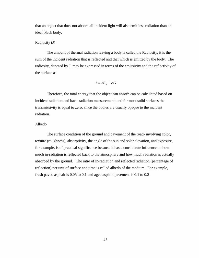
Radiosity (J)

The amount of thermal radiation leaving a body is called the Radiosity, it is the

sum of the incident radiation that is reflected and that which is emitted by the body. The

radiosity, denoted by J, may be expressed in terms of the emissivity and the reflectivity of

the surface as

GEJ b ρε +=

Therefore, the total energy that the object can absorb can be calculated based on

incident radiation and back-radiation measurement; and for most solid surfaces the

transmissivity is equal to zero, since the bodies are usually opaque to the incident

radiation.

Albedo

The surface condition of the ground and pavement of the road- involving color,

texture (roughness), absorptivity, the angle of the sun and solar elevation, and exposure,

for example, is of practical significance because it has a considerate influence on how

much in-radiation is reflected back to the atmosphere and how much radiation is actually

absorbed by the ground. The ratio of in-radiation and reflected radiation (percentage of

reflection) per unit of surface and time is called albedo of the medium. For example,

fresh paved asphalt is 0.05 to 0.1 and aged asphalt pavement is 0.1 to 0.2

26

3.3 Finite Element Analysis Approach

The finite element analysis is a numerical method for solving problems of

engineering and mathematical physics. For the problems involving complicated

geometries, loadings, and materials properties, it is generally not possible to obtain

analytical mathematical solutions. The finite element formulation of the problem results

in a system of simultaneous algebraic equation for simulation, rather than requiring the

solution of differential equations. These numerical methods yield approximate values of

the unknowns at discrete numbers of points in the continuum (23).

The heat transfer problem can be analyzed based on conservation of energy and

Fourier’s law of heat conduction.

Heat Conduction (Without Convection)

By conservation of energy

AdtqUQAdxdtAdtqor

EUEE

dxxx

outgeneratedin

++∆=+

+∆=+

Where Ein is the energy entering the control volume, ΔU is the change in stored energy,

qx is the heat conducted (heat flux) into the control volume at surface edge x, qx+dx

By Fourier’s law of heat conduction,

is the

heat conducted out of control volume at the surface edge x+dx, t is time, Q is the internal

heat source, and A is the cross-sectional area.

dxdTKq xxx −=

Where Kxx

The change in stored energy can be expressed by

is the thermal conductivity in the x direction, T is the temperature, 𝑑𝑑𝑇𝑇𝑑𝑑𝑥𝑥

is the

temperature gradient.

dTAdxcU )(ρ=∆

27

Where c is the specific heat and ρ is the mass density.

One-dimensional heat conduction equation as

tTcQ

xTK

x xx ∂∂

=+

∂∂

∂∂ ρ

For steady state, any differentiation with respect to time is equal zero,

0=+

∂∂

∂∂ Q

xTK

x xx

For constant thermal conductivity and steady state,

02

2

=+

∂∂ Q

xTK xx

The boundary conditions are of the form

T = TB on S

Where T

1

B represents a known boundary temperature and S1

Where S

is a surface where

temperature is known, and

𝑞𝑞𝑥𝑥∗ = −𝐾𝐾𝑥𝑥𝑥𝑥𝑑𝑑𝑇𝑇𝑑𝑑𝑥𝑥

= 𝑖𝑖𝑎𝑎𝑟𝑟𝑎𝑎𝑟𝑟𝑚𝑚𝑟𝑟𝑟𝑟 𝑎𝑎𝑟𝑟 𝑆𝑆2

2

Convective heat transfer

is a surface where the prescribed heat flux 𝑞𝑞𝑥𝑥∗ or temperature gradient is

known, and on an insulated boundary 𝑞𝑞𝑥𝑥∗ = 0.

For a conducting solid in contact with a fluid, if heat transfer is taking place, the

fluid will be in motion either through external pumping action (forced convection) or

through the buoyancy forces created within the fluid by the temperature differences

within it (natural or free convection).

28

For conservation of energy

( ) PdxdtqAdtqdTAdxcQAdxdtAdtq hdxxx ++=+ +ρ

Heat transfer convection is

( )∞−= TThqh

Where h is the heat-transfer or convection coefficient, T is the temperature of the solid

surface, 𝑇𝑇∞ is the temperature of the fluid, P is the perimeter around the constant cross-

sectional area A.

Heat Conduction (with convection)

( )∞−+∂∂

=+

∂∂

∂∂ TT

AhP

tTcQ

xTK

x xx ρ

With possible boundary conditions on (1) temperature, (2) temperature gradient,

and/or (3) loss of heat by convection from the ends of the one-dimensional body,

)( ∞−=− TThdxdTK xx

Total heat transfer from simulated heat flux into the object (asphalt pavement) can

be defined as

)()()( 44sairsaircirradiant TTTThqTk −+−+−=∆ εσ

Conduction heat transfer

dTTkq sd

conduction−

−=

Where qirradiant incident radiation, k is thermal conductivity of the material, Td is the

temperature at distance x, Ts

is the surface temperature, d is the total length.

29

Heat Radiation

The emitted radiation intensity from the object (pavement) surface to its

surroundings is calculated as

)( airsrradiation TThq −=

))(( 22airsairsr TTTTh +−= εσ

)( 44airsradiation TTq −= εσ

Where qradiation = incident radiation, hr is heat transfer coefficient, ε is the emissivity of

the material, σ = Stefan-Boltzmann constant = 5.68x10-8W/(m2·K4), Ts is surface

temperature in Kelvin, Tair

is air temperature Kelvin.

30

CHAPTER 4

THERMAL PROPERTIES AND TEMPERATURE OF EXISTING ASPHALT

PAVEMENT

4.1 Introduction

It is a common knowledge that asphalt pavements get heated up by sunlight, and

the thermal conditions which the pavements are exposed to greatly affect the performance

and longevity of the pavement. Research has shown that there is a temperature

distribution inside asphalt pavements, in the different layers, which are in many cases

made up of different materials.

The temperature distribution along the depth actually depends on the properties of

these different layers – the temperature at any layer is affected significantly by the

thermal properties of the layers above and below it. Thus, the temperature distribution in

a full depth asphalt pavement will be different from, for example, an asphalt pavement

with an aggregate base, even though the asphalt mixtures/materials in the two pavements

are the same.

This is of practical significance considering the wide variety of materials that are

currently being used as base material in both highway and airfield pavements.

4.2 Objective

The objectives of this chapter were to:

1. Investigate the temperature distribution along the depth of asphalt pavements with

six different base layers with laboratory experiments.

2. Build statistical models to predict the temperature in different base layers.

3. Model the temperature distribution, using principles of thermodynamics in

different pavements and determine appropriate values of thermal properties of the

different layers.

4.3 Methodology

The six existing pavement samples used were described in Table 4-1 and Figure

4-1 shows photos of the samples. The different base layer materials considered in this

phase were conventional Hot Mix Asphalt (HMA) – one with a bigger Nominal

Maximum Aggregate Size (NMAS) compared to the surface course and another with the

same NMAS, Plant Mixed Reclaimed Asphalt Pavement (PMRAP, RAP mixed with

31

asphalt emulsion), foamed asphalt mix, cement treated base and a polymer modified

HMA. Two of the samples were from airport pavements, while the rest were from

highway pavements. The highway pavements consist of standard wearing and binder

course HMA and different reclaiming material as base course, with one HMA base

course. Of the two airport pavement samples, one consists of standard FAA specified

P401 mix wearing, binder and base courses (these are actually a number of overlays),

while the other consists of Fuel Resistant (FR) wearing course over polymer modified

binder course.

A typical test consisted of the followings steps.

1. Set up the halogen lamp with a timer programmed to operate on 12 hours on and

12 hours off cycle.

2. Position the sample over the base and make all the appropriate connections for

thermocouples.

3. Start the data acquisition system.

4. Switch on the halogen lamp.

5. Continuously collect temperature data from all thermocouple locations.

6. Repeat the above steps to go through several cycles of temperature.

32

Table 4-1 Types of pavements considered

Pavements Sample/description Thickness Bulk Specific Gravity

Highway-HMA layers over HMA base with different NMAS

G – Wearing (9.5 NMAS) and two base courses (12.5 and/or 19mm); 9.5mm NMAS mix with 6% PG 64-28 binder; 12.5 NMAS mix with 5.9 % PG 64-28 binder; 19mm NMAS mix with 5.1% PG 64-28 binder

(35mm over 40mm over 125mm) Sample - 72mm of wearing +binder HMA over 115mm of base

Top layer: 2.277 Middle Layer: 2.342 Bottom Layer: 2.321

Highway-HMA layers over PMRAP base

S (9.5mm over 12.5mm NMAS over PMRAP base); PMRAP – RAP with 3.5% emulsion and 1.3% cement; 9.5 and 12.5mm mixes as described for G sample

(30mm over 40mm over 75mm) Sample – 63 mm of HMA over 75 mm of PMRAP

Top layer+ Middle Layer 2.377 Bottom Layer: 2.084

Highway-HMA layers over Foamed Asphalt base

M– (9.5 mm over 9.5 mm over foamed asphalt base); foamed asphalt contained 3.1 % binder and 1.4% cement; 9.5 mm mix as described for G sample

(30mm over 30mm) over 150mm Sample – 55 mm of HMA over 135 mm of foamed asphalt

Top layer+ Middle Layer 2.284 Bottom Layer 2.067 1.975

Highway-HMA layers over cement treated base

R (9.5mm over 12.5 mm over Cement treated base); full depth reclaimed base with 4% cement; 9.5 and 12.5mm mixes as described for G sample

(32mm over 45mm over 200mm) Sample – 70mm of HMA over 165mm of cement treated base


Airport-HMA layers of same NMAS – three lifts of P 401

P401-Three layers of RAP-P401 layers; 19mm maximum size mix with 18 % RAP, 1% lime, and 5.2% PG 64-28 binder

Sample - 54mm over 70mm over 80mm over 94mm


Airport-HMA layers of different types two lifts -

(FR) Fuel Resistant ½ inch NMAS mix over ¾ inch NMAS polymer modified (PM) binder mix over existing HMA or Macadam; FR – 12.5 mm maximum size mix with 7% PG 88-22 Fuel Resistant binder PM – 19 mm maximum size mix with 6% PG 82-22 PM binder

Sample – 40 mm of FR over 53mm of PM over 59 mm of existing P401 mix


Note: All binders are PG 64-28 grade, unless mentioned otherwise

33

Figure 4-1 Six existing highway samples

34

4.4 Laboratory Parameters Measurement

Heat Flux Measurement

The basic test set up first proposed by Luca and Mrawira (11) and used by

Nazarian and Alvarado (24) has been utilized in this study. It consists of a pavement

sample encapsulated within Styrofoam (thermal conductivity = 0.029 – 0.033W/m∙K).

A halogen lamp positioned over the sample was used to raise the temperature of

the sample (Figure 4-2), and temperatures were recorded constantly over the duration of

the tests. Each sample was fitted with thermocouples at different depths as well as on the

surface. Figure 4-3 shows the location of the thermocouples for the different samples

(Appendix A).

Figure 4-2 Laboratory testing setup

Halogen Lamp

Computer

Data Acquisition System

Timer

Sample

Thermocouple

35

Figure 4-3 Location of thermocouples in different samples

T1

Sample 401

T2 T3

T4

T5

T6

T1

HMA

FR-HMA

Sample FR/PM Sample G

Foamed Aphalt PMRAP

HMA

layers

Sample S Sample M

HMA

Layers

Sample R

T2 HMA

T3

T4 Cement

treated

T5

T6

T1 T1

T2 T2

T3 HMA

layers T3

T4 T4

T5 T

T6 T6

T1 T1

T2 T2 T3 T3 T4

T4 HMA

Layers T5 PM-HMA T5

T6 T6

Note: T1-T6 – thermocouples 1 through 6; PMRAP- plant mixed RAP with emulsion; FR-HMA- fuel resistant HMA; PM-HMA- polymer modified HMA

36

Radiation from the halogen lamp was measured by using a CMP-3 pyranometer,

and the radiation was measured indirectly by placing a piece of aluminum foil on the

surface of the HMA sample to measure the reflected radiation. The emissivity of the

aluminum foil is 0.03 which means it would reflect 97% of radiation emitted from the

halogen lamp Figure 4-4.

Figure 4-4 Halogen lamp heat radiation measurement

The halogen lamp (100W) was positioned 1.1m above the sample, primarily on

the basis of convenience in setting up the experiment. The incident radiation from the

lamp at this level was found to be 500W/m2

Two samples were also tested with wind, using a fan held close to the sample.

The position of the fan was adjusted to produce a wind speed of 4.45m/s (10mph), as

measured with an anemometer (Figure 3-4).

, as measured with a pyranometer.

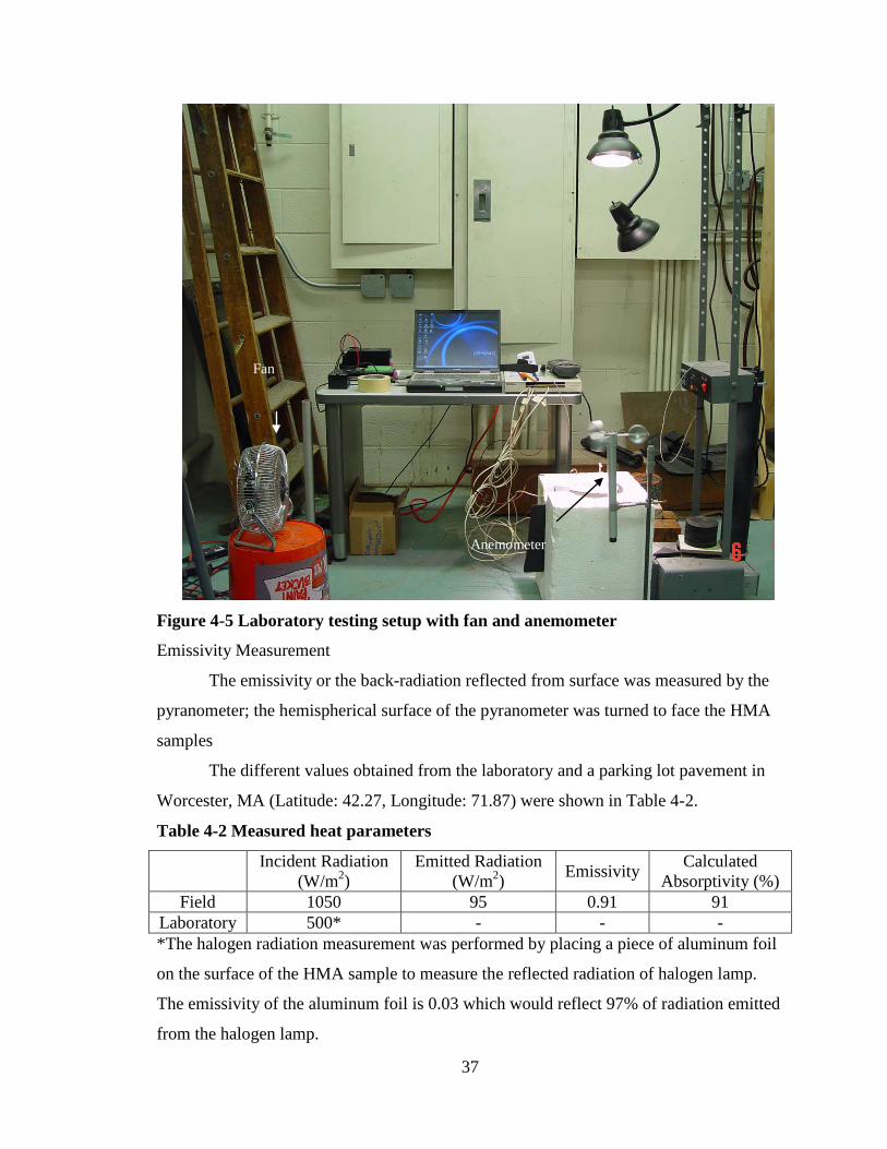
37

Figure 4-5 Laboratory testing setup with fan and anemometer

Emissivity Measurement

The emissivity or the back-radiation reflected from surface was measured by the

pyranometer; the hemispherical surface of the pyranometer was turned to face the HMA

samples

The different values obtained from the laboratory and a parking lot pavement in

Worcester, MA (Latitude: 42.27, Longitude: 71.87) were shown in Table 4-2.

Table 4-2 Measured heat parameters

Incident Radiation (W/m2

Emitted Radiation (W/m) 2 Emissivity )

Calculated Absorptivity (%)

Field 1050 95 0.91 91 Laboratory 500* - - - *The halogen radiation measurement was performed by placing a piece of aluminum foil

on the surface of the HMA sample to measure the reflected radiation of halogen lamp.

The emissivity of the aluminum foil is 0.03 which would reflect 97% of radiation emitted

from the halogen lamp.

Fan

Anemometer

38

The total reflected radiation can be calculated as

2/500)(

48597.0485

mWxRadiationxx

=

=⇒=ρ

Absorptivity calculation:

Field radiation:

91.009.011

09.01050

95

=−==+

==

αρα

ρ

The emissivity ε can be obtained by Kirchhoff's law of thermal radiation:

emissivity equals absorptivity (for an object in thermal equilibrium). Therefore,

emissivity of field pavement is 0.91, and this was used for laboratory samples.

This value was checked by testing each sample for emissivity. The pyranometer

was positioned to face the surface of the HMA and the back radiation was measured. The

results are shown in Table 4-3. Note that the measured values are fairly close to 0.91. The

0.91 value was used instead of the different measured values since it was suspected that

during this testing the pyranometer created a small shadow on the surface of the samples

and hence the measured values could be slightly different than real values.

Table 4-3 Measured emissivity values

Sample

Temperature (°C)

Radiation (W/m2

) ε (air)

ε (HMA)

T1 T2 G 29.14 41.08 79.35 0.16 0.84 S 33.00 44.89 82.01 0.16 0.84 M 31.53 41.45 66.81 0.13 0.87 R 34.04 42.17 55.61 0.11 0.89

P401 29.36 39.63 67.84 0.14 0.86 FR 30.08 41.3 74.99 0.15 0.85

T1- thermocouple 25 mm above the surface in air, T2- thermocouple on the surface

39

4.5 Experiment Results

The temperature data from each sample was analyzed to determine the

temperature profile along the depth and different times. For all of the samples, the

maximum temperature along the depth was recorded by the thermocouple located 25mm

below the surface.

Table 4-4 G Sample - Highway-HMA layers over HMA base with different NMAS

1st 2nd 3rd 4th 5th 6th 7th Time (mins) 720 2160 3600 5040 6480 7920 9360 Depth (m) T (°C) T(°C) T(°C) T(°C) T(°C) T(°C) T(°C) MEAN STDev

0 41.21 39.07 41.23 39.08 37.98 39.07 38.85 39.50 1.24 -0.0254 47.87 47.79 47.40 45.92 44.19 44.29 44.23 45.96 1.73

-0.05715 44.21 44.25 43.97 42.91 41.47 41.33 41.09 42.75 1.43 -0.1016 38.25 38.34 38.22 37.49 35.89 36.07 35.68 37.13 1.21 -0.1524 35.19 35.15 35.33 34.54 33.10 33.16 32.98 34.21 1.09

Figure 4-6 G Sample temperature distribution (7-days cycle)

-0.18

-0.16

-0.14

-0.12

-0.1

-0.08

-0.06

-0.04

-0.02

0

30 35 40 45 50

Dep

th (m

)

Temperature °C

G Sample Temperature Distribution (7- Days Cycle)

1st Day

2nd Day

3rd Day

4th Day

5th Day

6th Day

7th Day

Mean

40

Table 4-5 S Sample -HMA layers over PMRAP base

1st 2nd 3rd 4th 5th 6th 7th Time (mins) 720 2160 3600 5040 6480 7920 9360 Depth (m) T(°C) T(°C) T(°C) T(°C) T(°C) T(°C) T(°C) Mean STDev

0 47.44 48.50 48.15 48.70 46.68 47.42 46.45 47.62 0.87 -0.0254 47.31 50.28 49.91 49.53 49.17 49.10 48.15 49.06 1.03

-0.041275 46.01 49.49 49.10 48.81 48.51 48.33 47.41 48.24 1.18 -0.079375 40.87 45.91 45.52 45.26 45.08 44.90 43.71 44.46 1.73 -0.10795 38.39 43.99 43.82 43.43 43.17 43.07 41.99 42.55 1.95

Figure 4-7S Sample temperature distribution (7-days cycle)

-0.12

-0.1

-0.08

-0.06

-0.04

-0.02

0

30 35 40 45 50 55

Dep

th (m

)

Temperature °C

S Sample Temperature Distribution (7- Days Cycle)

1st Day

2nd Day

3rd Day

4th Day

5th Day

6th Day

7th Day

Mean

41

Table 4-6 M Sample- HMA layers over Foamed Asphalt base


0 43.88 44.13 46.10 44.72 44.47 43.26 43.27 44.26 0.98 -0.0254 47.02 48.46 51.83 50.78 50.57 49.92 49.75 49.76 1.59 -0.0508 45.90 47.42 49.85 48.68 48.49 47.95 47.76 48.01 1.22

-0.06985 40.23 41.90 43.31 42.31 42.11 41.55 41.41 41.83 0.94 -0.10795 36.72 38.15 39.54 38.65 38.35 37.98 37.86 38.18 0.85

Figure 4-8 M Sample temperature distribution (7-days cycle)

-0.12

-0.1

-0.08

-0.06

-0.04

-0.02

0

30 35 40 45 50 55

Dep

th (m

)

Temperature °C

M Sample Temperature Distribution (7- Days Cycle)

1st Day

2nd Day

3rd Day

4th Day

5th Day

6th Day

Mean

7th Day

42

Table 4-7 R Sample- HMA layers over cement treated base


0 44.80 43.88 42.19 42.86 42.97 44.21 41.78 43.24 1.10 -0.0254 47.68 47.83 48.43 48.05 48.84 48.38 48.50 48.25 0.41 -0.0508 46.60 46.89 47.52 47.12 47.85 47.50 47.44 47.28 0.43

-0.107995 42.47 42.93 43.61 43.03 43.69 43.50 43.33 43.22 0.44 -0.17145 38.61 39.13 39.82 39.17 39.85 39.69 39.60 39.41 0.46

Figure 4-9 R Sample temperature distribution (7-days cycle)

-0.2

-0.18

-0.16

-0.14

-0.12

-0.1

-0.08

-0.06

-0.04

-0.02

0

30 35 40 45 50

Dep

th (m

)

Temperature °C

R Sample Temperature Distribution (7- Days Cycle)

1st Day

2nd Day

3rd Day

4th Day

5th Day

6th Day

7th Day

Mean

43

Table 4-8 P401 Sample- HMA layers of same NMAS


0 41.86 42.40 42.55 44.76 45.01 44.43 44.73 43.68 1.34 -0.0254 45.70 44.38 45.36 46.83 46.52 46.21 46.67 45.95 0.87 -0.09525 37.09 36.00 36.93 37.92 37.85 37.75 37.96 37.36 0.73 -0.1651 33.10 32.23 32.98 33.63 33.67 33.60 33.76 33.28 0.55 -0.2286 31.38 30.77 31.37 31.83 32.07 31.95 32.03 31.63 0.48

Figure 4-10 P401 Sample temperature distribution (7-days cycle)

-0.24

-0.22

-0.2

-0.18

-0.16

-0.14

-0.12

-0.1

-0.08

-0.06

-0.04

-0.02

0

30 35 40 45 50

Dep

th (m

)

Temperature °C

P401 Temperature Distribution (7- Days Cycle)

1st Day

2nd Day

3rd Day

4th Day

5th Day

6th Day

7th Day

Mean

44

Table 4-9 FR Sample- HMA layers of different types two lifts


0 43.12 44.86 43.16 45.35 43.27 41.27 42.62 43.38 1.37 -0.0254 47.54 47.99 47.31 48.58 47.87 47.14 47.20 47.66 0.52 -0.0508 44.67 45.19 44.82 45.82 45.06 44.51 44.47 44.93 0.47

-0.06985 43.42 44.24 43.75 44.73 43.87 43.38 43.36 43.82 0.51 -0.10795 41.31 41.98 41.77 42.37 41.73 41.06 41.21 41.63 0.47

Figure 4-11 FR Sample temperature distribution (7-days cycle)

-0.12

-0.1

-0.08

-0.06

-0.04

-0.02

0

30 35 40 45 50

Dep

th (m

)

Temperature °C

FR Sample Temperature Distribution (7- Days Cycle)

1st Day

2nd Day

3rd Day

4th Day

5th Day

6th Day

7th Day

Mean

45

Figure 4-12 showed a plot of temperatures versus depth for the different samples

at the end of the seventh heating cycle.

Figure 4-12 6 Samples temperature distribution at end of 7th

heating cycle

-0.2

-0.18

-0.16

-0.14

-0.12

-0.1

-0.08

-0.06

-0.04

-0.02

0

30 35 40 45 50 55

Dep

th (m

)

Temperature °C

Temperature at the End of 7th Heating Cycle

G

S

M

R

P401

FR

46

4.6 Statistical Approach of Determining Temperature at Specific Location

To predict the maximum temperature for each sample (mix) on the basis of

“known” or “measurable” temperatures, statistical analyses were conducted to build

models relating the maximum subsurface temperature to air and surface temperature.

These models were developed on the basis of one heating cycle data only. The equations

were shown in Table 4-10, which also included the equations developed for P401 and M

samples, with and without wind.

To predict the temperature in the “base” course, statistical models were developed

relating the base temperature to surface and air temperatures for each sample. These were

also shown in Table 4-10. Temperature limits of each equation were also shown. Note

that no attempt was made to compare the maximum temperatures for the different

samples, since the air temperatures in the laboratory were slightly different for the

different samples.

As expected, for each sample, the model for the temperature at a depth of 25mm

was different from the model for the temperature at the midpoint of the base. Also, the

coefficients for the equations for the different samples for temperature at a depth of

25mm were quite different. The different temperature profiles were no doubt affected by

the thermal properties of the different materials. The primary objective of presenting the

equation in Table 4-10 was to show the differences in the coefficients.

47

Table 4-10 Equation from statistical analysis

Sample

Model for prediction of maximum temperature, in the HMA layer, based on one heating cycle

Model for prediction of temperature at the mid-point of base layer, based on one heating cycle

P401/no wind TAT

:25.8 to 36.2 °C S

:25.8 to 41.9 °C T20mm= 1.700.92*TA+1.81*T

S Tbase= 14.15-1.00*TA+1.36*T

S

P401/10 mph wind TAT

:26.1 to 27.5 °C S

:25.9 to 33.3 °C T20mm= 2.48– 0.73*TA+1.52*T

S

Tbase = -7.52-0.02*TA+1.12*T

S

R TAT

:26.6 to 38.5 °C S

:27.6 to 45.3 °C T20mm= 0.16– 1.50*TA+2.36*T

S

Tbase= -3.69–1.48*TA+2.28*T

S

S TAT

:26.9 to 37.3 °C S

:26.7 to 47.9 °C T20mm = 6.05– 0.91*TA+1.56*T

S

Tbase= 18.35-1.29*TA+1.47*T

S

G TAT

:23.3 to 36.4 °C S

:25.4 to 51.2 °C T20mm= -18.41–0.45*TA+1.59*T

S

Tbase= -22.23-0.35*TA+1.52*T

S

FR over PM TAT

:24.7 to36.2 °C S

:25.3 to 43.9 °C T20mm= -2.65–1.19*TA+2.11*T

S Tbase= 0.18–1.45*TA+2.19*T

S

M TAT

:24.6 to 33.9 °C S

:24.5 to 43.9 °C T20mm= -0.97– 0.98*TA+1.87*T

S

Tbase= 9.02–1.57*TA+1.95*T

S

M/10 mph wind TAT

:23.9 to 26.9 °C S

:24.5 to 31.9 °C T20mm= -8.97– 0.46*TA+1.66*T

S

Tbase= -28.46+1.09*TA+0.86*T

S

Where TA= air temperature, °C; and TS

= surface temperature, °C.

48

4.7 Finite Element Analysis/Modeling

The heating of each sample was modeled using the finite element analysis. The

objective of finite element modeling was to “backcalculate” the unknown thermal

conductivity and heat capacity of the different layers for existing highway and airport

samples. These parameters were required as inputs for consideration of the effect of the

environment in the mechanistic-empirical pavement design process, using the Enhanced

Integrated Climatic Model (EICM) (25).

Heat transfer module from COMSOL Multiphysics software (26) was used for

simulating the heat transfer process and predicting the thermal properties of the asphalt

mix samples.

There were four main components that required to be identified in order to model

the heat transfer process: sub-domain, boundary condition, mesh size, and solver

parameter. Subdomains were defined based on the thermal properties, densities and

initial temperatures of each layer. The boundary conditions for the samples were assumed

as fully insulated except the top surface boundary, where natural convection with laminar

air flow condition was assumed. The model allowed heat energy transfer in the

downward (-z) direction. There were five parameters that were required for boundary

condition inputs: heat flux, heat transfer coefficient, ambient temperature, surface

temperature, and surface emissivity.

For modeling, the global mesh size was set to predefined normal size which

consisted of 3,436 elements for sub-domains, boundaries, edges, and nodes. The solver

parameters were set to time dependant analysis with steps of 900 seconds from 0 to

43,200 seconds for one heating cycle. Examples of a model and results were shown in

Figure 4-13 and 4-14.

Figure 6. Plots for all samples

49

Figure 4-13 Mesh generated from COMSOL

Figure 4-14 COMSOL simulation result

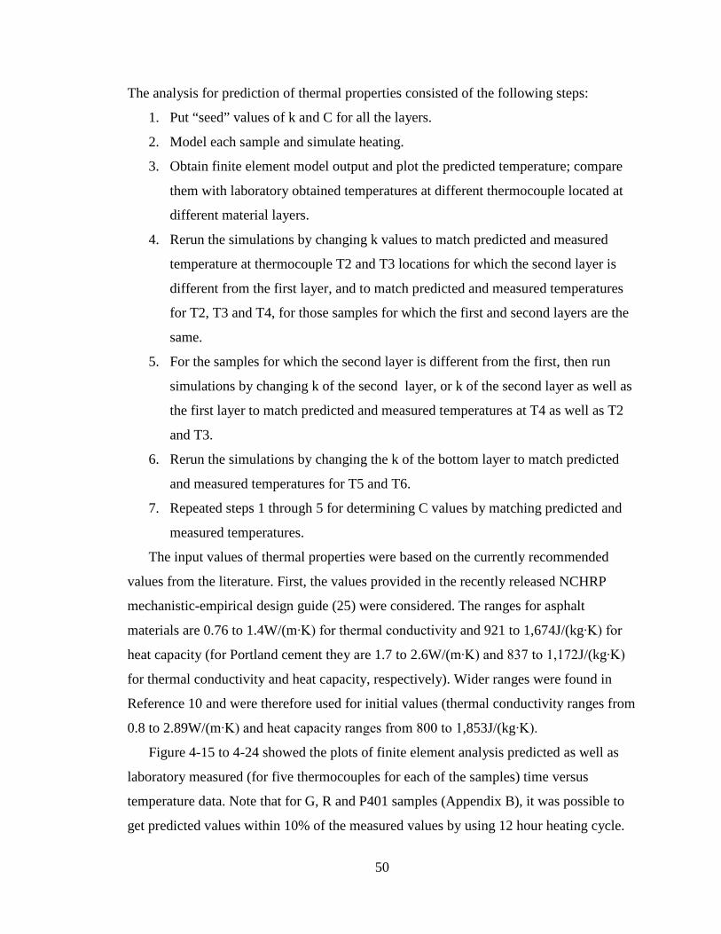
50

The analysis for prediction of thermal properties consisted of the following steps:

1. Put “seed” values of k and C for all the layers.

2. Model each sample and simulate heating.

3. Obtain finite element model output and plot the predicted temperature; compare

them with laboratory obtained temperatures at different thermocouple located at

different material layers.

4. Rerun the simulations by changing k values to match predicted and measured

temperature at thermocouple T2 and T3 locations for which the second layer is

different from the first layer, and to match predicted and measured temperatures

for T2, T3 and T4, for those samples for which the first and second layers are the

same.

5. For the samples for which the second layer is different from the first, then run

simulations by changing k of the second layer, or k of the second layer as well as

the first layer to match predicted and measured temperatures at T4 as well as T2

and T3.

6. Rerun the simulations by changing the k of the bottom layer to match predicted

and measured temperatures for T5 and T6.

7. Repeated steps 1 through 5 for determining C values by matching predicted and

measured temperatures.

The input values of thermal properties were based on the currently recommended

values from the literature. First, the values provided in the recently released NCHRP

mechanistic-empirical design guide (25) were considered. The ranges for asphalt

materials are 0.76 to 1.4W/(m∙K) for thermal conductivity and 921 to 1,674J/(kg∙K) for

heat capacity (for Portland cement they are 1.7 to 2.6W/(m∙K) and 837 to 1,172J/(kg∙K)

for thermal conductivity and heat capacity, respectively). Wider ranges were found in

Reference 10 and were therefore used for initial values (thermal conductivity ranges from

0.8 to 2.89W/(m∙K) and heat capacity ranges from 800 to 1,853J/(kg∙K).

Figure 4-15 to 4-24 showed the plots of finite element analysis predicted as well as

laboratory measured (for five thermocouples for each of the samples) time versus

temperature data. Note that for G, R and P401 samples (Appendix B), it was possible to

get predicted values within 10% of the measured values by using 12 hour heating cycle.

51

For the S, M and FR samples (Appendix B) this was not possible, and the back-

calculation was done by remodeling and reanalyzing the predicted data for 6 hours of

heating.

Figure 4-15 G sample temperature at T2 (finite element analysis vs. laboratory

results)


results)

0

10

20

30

40

50

60

70

0 60 120 180 240 300 360 420 480 540 600 660 720

Tem

pera

ture

°C

Time (mins)

G Sample T2 (k=1.0W/m·K, C=1100J/kg)

LAB

FE

0

10

20

30

40

50

60

70

0 60 120 180 240 300 360 420 480 540 600 660 720

Tem

pera

ture

°C

Time (mins)


LAB

FE

52


results)


results)

0

10

20

30

40

50

60

70

0 60 120 180 240 300 360 420 480 540 600 660 720

Tem

pera

ture

°C

Time (mins)

G Sample T4(k=1.0W/m·K, C=1100J/kg)

LAB

FE

0

10

20

30

40

50

60

70

0 60 120 180 240 300 360 420 480 540 600 660 720

Tem

pera

ture

°C

Time (mins)


LAB

FE

53


results)

Figure 4-20 S sample temperature at T2 (finite element analysis vs. laboratory

results)

0

10

20

30

40

50

60

70

0 60 120 180 240 300 360 420 480 540 600 660 720

Tem

pera

ture

°C

Time (mins)


LAB

FE

0

10

20

30

40

50

60

0 60 120 180 240 300 360

Tem

pera

ture

°C

Time (mins)

S Sample T2 (k=1.3W/m·K, C=1200J/kg)

LAB

FE

54


results)


results)

0

10

20

30

40

50

60

0 60 120 180 240 300 360

Tem

pera

ture

°C

Time (mins)


LAB

FE

0

10

20

30

40

50

60

0 60 120 180 240 300 360

Tem

pera

ture

°C

Time (mins)


LAB

FE

55


results)


results)

0

10

20

30

40

50

0 60 120 180 240 300 360

Tem

pera

ture

°C

Time (mins)


LAB

FE

0

10

20

30

40

50

0 60 120 180 240 300 360

Tem

pera

ture

°C

Time (mins)


LAB

FE

56

4.8 Discussion

The back-calculated thermal conductivity (k), heat capacity (C), and thermal

diffusivity (α) values for the different materials (layers) were shown on the respective

samples in Table 4-11. Note that HMA and the other materials are all anisotropic and

therefore the thermal properties are not the same in any direction – the estimated thermal

properties indicated the effective and overall thermal property for the different layers.

The lengths of the different samples were different; this had affected the results

from modeling as well as laboratory measurements. The study was carried out to estimate

thermal properties of different layers in typical pavements. Therefore, these results are

valid for the different materials and layers as long as they are present in a

structure/thickness similar to those used in this chapter.

It was interesting to note from Table 4-11 that similar HMA mixes presented in

different structures (that is with different base layers) showed different “effective”

thermal properties. In their 2006 paper, Côté and Konrad (27) presented a practical

approach of estimating thermal conductivity of pavement granular materials. Their

method linked dry and saturated thermal conductivities through a set of empirical

parameters, and one could estimate the thermal conductivity by using these parameters,

as well as saturation and thermal conductivity of the solid particles, which could be

estimated by considering the proportion of different minerals presented in the granular

particles and their respective thermal conductivities. They also provided data which

showed that thermal conductivities were inversely related to porosity of the soil particles.

One important point they noted was that for dry soils, the thermal conductivity

was more sensitive to microstructure and/or particle type and less on the thermal

conductivity of the solid particles. Since all of the mixes considered here were dry, it

could be expected that mixes with similar aggregates, but different gradations and

densities would show different thermal conductivities.

57

Table 4-11 Backcalculated thermal properties of existing asphalt pavement samples

Materials

Thermal

Conductivity

W/(m∙K)

Heat Capacity

J/(kg∙K)

Thermal

Difussivity

(m2/s)

Surface+Binder

HMA over similar HMA base (G) 1.6 1200 5.77e-07

HMA over Emulsion treated RAP base (S) 1.3 1200 4.55e-07

HMA over Cement treated base (R) 1.8 1800 4.59e-07

HMA over foamed asphalt (M) 1.5 1800 3.62E-07

HMA over coarser HMA base (P401) 1.0 1100 3.64E-07

Fuel resistant HMA over Polymer Modified

HMA Base (FR) 1.5 1200 4.89e-07

Base

HMA Base (G) 1.6 1200 5.60e-07

Emulsion treated RAP Base (S) 1.3 1200 5.19e-07

Cement Treated Base (R) 1.5 1400 5.42e-07

Foamed Asphalt Base (M) 1.5 1800 4.09e-07

HMA Base (P401) 1.1 1400 3.18e-07

Polymer Modified HMA Base (FR) 1.6 1200 5.40e-07

Note that because of the presence of asphalt binder in significant amount (5-7%),

the use of the procedure outlined in Reference 24 may be somewhat impractical at this

time, especially since the empirical parameters that are needed in this procedure have not

been developed yet.

In this chapter, the backcalculated thermal conductivity and heat capacity values

at the different thermocouple locations were adjusted until the predicted and measured

temperatures at all thermocouple were within ± 10% of each other. Therefore, the

analysis was affected significantly by the thermocouple locations – which were the same

for the surface layers of all of the samples (surface, and 25mm below the surface), but not

in the base layers. The base thermocouples were placed in the base layers at the third

points – one third and two third down from the surface+binder layer. The temperature

distribution throughout the depth of the base layer was measured. Therefore, the back-

58

calculated values were strictly valid for pavement structures which have the respective

materials at the depths which are present in the sampled pavements.

This could be considered as a drawback, but more importantly, it pointed out the

importance of estimating thermal properties of similar materials in conjunction with base

materials in different pavement structures. Thermal conductivity or heat capacity testing

(in the way conducted in this chapter) of surface+binder or base course only samples

would not yield the same values as obtained in this chapter, and would most likely be

also further away from the “effective” values. Obviously the best approach is using data

from in-place instrumentation. Since in-place instrumentation is relatively costly and

involves a significant amount of installation work, testing full-depth (or at least with base

layer) samples as done in this study is an alternative option. Furthermore, even though

Reference 22 recommends ASTM E1952, direct validation of thermal conductivity of a

composite material as HMA is very difficult.

59

CHAPTER 5

SMALL SCALE ASPHALT PAVEMENT TESTING

5.1 Introduction

The heat transfer from a pavement heated by solar energy can be enhanced by

using a high conductivity material as well as by using an insulating layer on the top that

would reduce reflectivity and emissivity. The amount of energy generated can also be

increased significantly by increasing the surface area exposed to the sun. To ensure that

the pavement is constructed using conventional equipment and techniques, and it is

sufficiently durable, the materials that can be used are mineral aggregates, asphalt binder

and additives, and the insulating layer on the top has to be either in the form of a powder

or a liquid. Accordingly, the effect of higher conductivity material, layers on the surface,

and surface area were evaluated in this chapter.

5.2 Objective

The objectives of this chapter were to evaluate:

1. Aggregate with high conductivity.

2. Partial replacement of granite aggregate with quartzite.

3. High conductivity material as additives.

4. Absorptivity enhancing paint.

5. Modified surface conditions.

6. Increased surface area of sample and copper pipe.

7. Controlled water inlet temperature and volume.

5.3 Methodology

The methodology of this chapter included finite element modeling, experiments

with small 150 mm diameter, 114 mm thick pavement samples (henceforth referred to as

small scale tests) (Hot Mix Asphalt, HMA samples, compacted using Superpave gyratory

compactor in the laboratory, and a dense graded HMA mix gradation and asphalt content;

all HMA used in this study had PG 64-28 grade asphalt binder).

The relative positions of the heating lamp over the HMA sample were selected to

provide 1,000W/m2 of radiation (Appendix C). The radiation 1,000W/m2 was used for

simulating the maximum summer time radiation in Worcester, MA area. The objective

60

was to investigate change of temperature in the water caused by conduction of heat from

a heated HMA sample for a time span of 6 hours, and as well to evaluate the effect of

thermal conductivity. The finite element analysis was used along with these preliminary

tests.

This chapter was a continuation of investigating of temperature distributions in

150 mm diameter pavement samples, which were subjected to heat radiation from a

halogen lamp. The experiment setup and test were categorized into five scenarios.

I. A 0.0508m (½”) diameter copper pipe was inserted inside the sample; the

other end of the copper pipe was placed in a small bath of water. Initially, the

copper pipe was used as the “heat exchanger” between the heated HMA

sample and the water in the bath. Thermocouples were positioned to the

sample at different heights, and the bath/inlet and outlets were connected to a

data acquisition system, which allowed continuous recording of temperature

(Appendix C). The following samples were analyzed:

1. 100% Quartzite mix.

2. 100% Limestone mix.

3. 100% Quartzite mix with tinted glass on the surface.

II. Modified initial water temperature and flow rate and complied asphalt samples

with increased diameter of copper pipe (Appendix C). The following samples

were analyzed:

4. 100% Quartzite with iced water (3mL/min).

5. 100% Quartzite mix with trapped iced water inside of cooper pipe.

6. Complied of 5 quartzite samples with 0.01905m (¾”) copper pipe.

III. Uniform granite and quartzite aggregate with various water flow rate was

pumped through the 0.00635m (¼”) diameter copper pipe, and used as the

heat exchanger. Thermocouples were positioned to the sample at different

heights, and the bath/inlet and outlets were connected to a data acquisition

system, which allowed continuous recording of temperature. (Appendix C).

The following samples were analyzed:

7. 100% Quartzite mix.

61

8. 100% Metagranodiorite mix.

9. 100% RAP mix.

IV. Partial replacement of granite aggregate with quartzite with various water flow

rate was pumped through the 0.00635m (¼”) diameter copper pipe.

Thermocouples were positioned to the sample at different heights, and the

bath/inlet and outlets were connected to a data acquisition system, which

allowed continuous recording of temperature. The following samples were

analyzed:

10. Quartzite with 22% copper mix.

11. Quartzite with 30% aluminum mix.

12. Quartzite with 50% RAP mix.

13. Quartzite with 75% RAP mix.

14. 67% Quartzite with 33% limestone mix.

V. Modified surface conditions on partial replacement of granite aggregate with

quartzite with various water flow rate was pumped through the 0.00635m (¼”)

diameter copper pipe. Thermocouples were positioned to the sample at

different heights, and the bath/inlet and outlets were connected to a data

acquisition system, which allowed continuous recording of temperature. The

following samples were analyzed:

15. Tinted glass on the surface of 78% quartzite with 22% copper mix.

16. Acrylic paint on the surface of 78% quartzite with 22% copper mix.

17. Tinted glass on the surface of 70% quartzite with 30% aluminum mix.

18. Chipped glass with asphalt mix on the 70% quartzite with 30%

aluminum mix.

62


The 10, 20, 40, 60, 80, and 100mL/min water flow rate were used to determine

the temperature difference between initial water temperature and outflow water

temperature except scenario I.

The delta T of each scenario used for comparison was based on 10mL/min with

60 minutes of time period because the temperature showed most significant difference at

this flow rate. The heat energy (power) generated from each flow rate can be calculated

by:

𝑄𝑄 = 𝑚𝑚𝐶𝐶𝑝𝑝𝛥𝛥𝑇𝑇

Where m is mass of water, Cp

Scenario I

is heat capacity of water; ΔT is temperature difference

between water inlet and outlet.

The quartzite aggregate, consisting of approximately 95% quartz and with traces

of hematite (giving it a pink color) was obtained from New Ulm quarry, MN. This

aggregate is currently used mainly for poultry and traction grit as well as for railroad

ballast and surface seal mix aggregates. The limestone aggregate, typically used in HMA

mixtures, was obtained from Calera, AL.

Two HMA samples were prepared, one each with quartzite and limestone

aggregates. Rise of temperature in water was noted from tests conducted with the small

scale experimental setup described above. The results (Table 5-1 and Figure 5-1) showed

that the sample with quartzite aggregate had a significantly higher temperature difference

(between original water temperature and final water temperature) compared to the

limestone aggregate mix. The comparison revealed that the higher heat capacity of

quartzite (1.5 times higher) and conductivity (2.5 times higher) were clearly beneficial in

heating water by extracting heat from depth inside the pavement (via copper pipe inserted

at a depth of 25mm). The water was heated by 10.13°C for the quartzite sample over 6

hours as opposed to 5.02°C for the limestone sample. This showed preliminary evidence

that altering the pavement material would allow higher amount of heat energy from the

pavement to be extracted for similar radiation conditions.

63

Table 5-1 Quartzite and Limestone mix temperature difference

Tinitial T(°C) final ΔT (°C) (°C) Watt, W 100% Quartzite mix 24.11 34.24 10.13 1.12 100% Limestone mix 23.81 28.83 5.02 0.55

The quartzite mix was then placed a tinted glass on its surface, and preformed the

same test procedure to investigate the improving heat transfer by modifying the surface

condition. The results (Table 5-2 and Figure 5-1) showed the delta T from quartzite with

tinted glass was slightly higher than just quartzite sample by 0.34°C, which meant that

the tinted glass would reduce the convective heat transfer from the surface of the sample,

and increased the heat transfer from asphalt sample to the water.

Table 5-2 Quartzite mix with and without placement of tinted glass temperature

difference

Tinitial T (°C) final ΔT (°C) (°C) Watt, W 100% Quartzite mix 24.11 34.24 10.13 1.12

100% Quartzite + Glass 23.39 33.87 10.47 1.16

Figure 5-1 Small scale testing (Scenario I) temperature difference ΔT

0.0

2.0

4.0

6.0

8.0

10.0

12.0

Asphalt Mix

Tem

pera

ture

Diff

eren

ce Δ

T °C

Small Scale Lab Sample

Small Scale Testing (Scenerio I) Temperature Difference ΔT

Case 1 (100% Quartzite)

Case 2 (100% Limestone)

Case 3 (100% Q+Tinted Glass)

64

Scenario II

The Figure 5-2 showed the most temperature difference was trapped iced water

inside of copper pipe; however, it did not generate the most power due to its small

volume. On the other hand, the compiled quartzite samples (Table 5-5) generated

approximately 6 times of power than other two samples (Table 5-3 and 5-4) because it

had most large surface area which increased higher heat transfer rate (Figure 5-3).

Scenario II

Table 5-3 100% Quartzite with iced water (3mL/min) temperature difference

Time (min) Tinitial T(°C) final ΔT (°C) (°C) 5 2.69 8.37 5.67 10 3.73 12.29 8.56 20 5.21 18.94 13.73 40 5.07 26.49 21.42 60 5.51 30.60 25.09 80 5.67 33.28 27.61

100 5.95 34.80 28.85 120 7.20 35.47 28.27

Table 5-4 100% Quartzite mix with trapped iced water inside of cooper pipe

temperature difference

Time (min) Tinitial T (°C) final ΔT (°C) (°C) 5 8.62 44.65 36.03 10 14.12 43.05 28.93 15 11.27 43.19 31.92 20 13.27 42.43 29.16 30 16.2 43.52 27.32

Table 5-5 Complied of 5 quartzite samples with 0.01905m (¾”) copper pipe


Flow Rate (mL/min) Tinitial T (°C) final ΔT (°C) (°C) 10 24.50 58.43 33.93 20 24.50 54.49 29.99 30 24.50 47.90 23.40 40 24.50 44.35 19.85 60 24.50 39.59 15.09 80 24.50 37.03 12.53 100 24.50 36.81 12.31

65

Figure 5-2 Small scale testing (Scenario II) temperature difference ΔT

Figure 5-3 Small scale testing (Scenario II) power generated

0.0

5.0

10.0

15.0

20.0

25.0

30.0

35.0

Asphalt Mix

Tem

pera

ture

Diff

eren

ce Δ

T °C

Small Scale Lab Samples

Small Scale Testing (Scenario II) Temperature Difference ΔT

Case 4 (Ice Water 3mL)

Case 5 (Traped Ice Water)

Case 6 (5 Q Compiled)

0.0

2.0

4.0

6.0

8.0

10.0

12.0

14.0

Asphalt Mix

Pow

ee (W

)


Small Scale Testing (Scenerio II) Power Generated

Case 4 (Ice Water 3mL)

Case 5 (Trapecd Ice Water)

Case 6 (5 Q Compiled)

66

Scenario III

Three HMA samples were prepared, one with 100% quartzite mix, one with

metagranodiorite mix, and one with 100 % locally available reclaimed asphalt pavement

(RAP) materials (with aggregate from bedrock characterized as biotite-quartz-plagioclase

granofels)). The Figure 5-4 showed the typical sample with thermocouple locations. The

final temperature readings of each flow rate were recorded when water temperature

remained stabilized. The results (Figure 5-5) showed that the delta T of 100% quartzite

mix (Table 5-6) from various flow rate were the highest among three. The Figure 5-6

showed that the most significant difference was at 10mL/min; even though the delta T of

100% RAP (Table 5-8) was slightly higher than 100% Wrentham (Table 5-7) at higher

flow rates, but the temperature difference is less than 1°C which could not be taken into

consideration. The Figure 5-7 also showed the power generated from 10mL/min for three

samples.

Figure 5-4Typical asphalt sample with thermocouples

T5- 91.6mm

T6- water outflow

T1-25.4mm above surface

T2- surface

T3- 25.4mm below surface

150mm

117m

m

¼”Copper Tube

Water Inflow

T4- 58.5mm

67

Table 5-6 100% Quartzite mix temperature difference

Flow Rate (mL/min) Tinitial T (°C) final ΔT (°C) (°C) 10 24.95 33.59 8.64 20 25.08 30.25 5.17 40 25.07 27.78 2.72 60 24.68 26.64 1.96 80 24.89 26.37 1.49 100 24.98 26.48 1.49

Table 5-7 100% Metagranodiorite mix temperature difference


Table 5-8 100% RAP mix temperature difference


68

Figure 5-5 Small scale testing (Scenario III) temperature vs. flow rate

0.0

1.0

2.0

3.0

4.0

5.0

6.0

7.0

8.0

9.0

10.0

0 10 20 30 40 50 60 70 80 90 100

Tem

pera

ture

Diff

eren

ce Δ

T, °

C

Flow Rate (mL/min)

Scenario III- ΔT vs. Flow Rate


Case 8 (100% Metagranodiorite)

Case 9 (100% RAP)

69

Figure 5-6 Small scale testing (Scenario III) temperature difference ΔT

Figure 5-7 Small scale testing (Scenario III) power generated

0.0

1.0

2.0

3.0

4.0

5.0

6.0

7.0

8.0

9.0

10.0

Asphalt Mix

Tem

pera

ture

Diff

eren

ce Δ

T °C


Scenerio III- ΔT at 10mL/min



Case 9 (100%RAP)

0.0

1.0

2.0

3.0

4.0

5.0

6.0

7.0

Asphalt Mix

Pow

er (W

)


Scenerio III- Power Generated at 10mL/min



Case 9 (100% RAP)

70

Scenario IV

Since a higher conductivity would help in obtaining a higher rate of energy

transfer, the metal with high conductivity, copper (k= 401 W/m·K) and aluminum

powder (k=250 W/m·K) were used by replacing about 22% and 30% of the quartzite

aggregate respectively. The both powders were mixed with the aggregates prior to mixing

with the asphalt binder. The samples were tested at different flow rates of water. A

comparison of delta T for samples with and without copper and aluminum was shown in

Figure 5-8 and 5-9. No significant increase in delta T was observed for the copper-HMA

and aluminum-HMA samples (Table 5-9 and 10). In fact, the delta T was reduced with

the introduction of copper and aluminum. This could be due to the fact that the copper

and aluminum powder were covered with asphalt during mixing and also was partially

oxidized during the heating of the aggregates prior to mixing.

Based on the results obtained, it was argued that a partial replacement of locally

available aggregates with quartzite aggregates would significantly increase delta T. Two

samples were prepared and tested to investigate one with 75% RAP and 25 % quartzite

aggregate and another one is with 50% RAP with 50% quartzite (Table 5-11 and 5-12).

As Figure 5-10, 5-11, 5-12 shows the addition of quartzite has a significant positive effect

on delta T.

Table 5-9 Quartzite with 22% copper mix temperature difference

Flow Rate (mL/min) T Tinitial ΔT final 10 24.50 31.46 6.96 20 24.50 28.65 4.15 40 24.50 26.84 2.34 60 24.50 26.35 1.85 80 24.50 26.17 1.67 100 24.50 26.16 1.66

Table 5-10 Quartzite with 30% aluminum mix temperature difference


71

Figure 5-8 Small scale testing (Scenario VI) effect of copper powder

Figure 5-9 Small scale testing (Scenario VI) effect of aluminum powder

0.0

1.0

2.0

3.0

4.0

5.0

6.0

7.0

8.0

9.0

10.0

0 10 20 30 40 50 60 70 80 90 100

Tem

pera

ture

Diff

eren

ce Δ

T, °

C

Flow Rate (mL/min)

Scenario VI- Effect of Copper Powder


Case10 (Q+22%Cu)

0.0

1.0

2.0

3.0

4.0

5.0

6.0

7.0

8.0

9.0

10.0

0 10 20 30 40 50 60 70 80 90 100

Tem

pera

ture

Diff

eren

ce Δ

T, °

C

Flow Rate (mL/min)

Scenario VI- Effect of Aluminum Powder


Case11 (Q+30%Al)

72

Table 5-11 Quartzite with 50% RAP mix temperature difference


Table 5-12 Quartzite with 75% RAP mix temperature difference


Table 5-13 67% quartzite with 33% limestone mix temperature difference


73

Figure 5-10 Small scale testing (Scenario VI) temperature vs. flow rate

0.0

1.0

2.0

3.0

4.0

5.0

6.0

7.0

8.0

9.0

0 10 20 30 40 50 60 70 80 90 100

Tem

pera

ture

Diff

eren

ce Δ

T, °

C

Flow Rate (mL/min)

Scenario VI- ΔT vs. Flow Rate

Case10 (Q+22%Cu)

Case11 (Q+30%Al)

Case 12 (50%Q+50%RAP)

Case 13 (25%Q+75% RAP)

Case 14 (67%Q+33% Limestone)

74

Figure 5-11 Small scale testing (Scenario VI) temperature difference ΔT

Figure 5-12 Small scale testing (Scenario VI) power generated

0.0

1.0

2.0

3.0

4.0

5.0

6.0

7.0

8.0

9.0

10.0

Asphalt Mix

Tem

pera

ture

Diff

eren

ce Δ

T °C


Scenerio VI- ΔT at 10mL/min

Case 10 (Q+22%Cu)

Case 11 (Q+30%Al)

Case 12 (50%Q+50%RAP)

Case 13 (25%Q+75%RAP)


0.0

1.0

2.0

3.0

4.0

5.0

6.0

7.0

Asphalt Mix

Pow

er (W

)


Scenerio VI- Power Generated at 10mL/min

Case 10 (Q+22% Cu)

Case 11 (Q+30% Al)

Case 12 (50%Q+50%RAP)

Case 13 (25%Q+75%RAP)


75

Scenario V

The tinted glass disk was placed on the quartzite sample with 22% copper powder

and 30% aluminum powder samples and observed the effect of modifying surface

conditions. The quartzite sample with 22% copper powder was then covered with a layer

of acrylic paint to observe any effect on delta T. As Figure 5-13, 5-14, and 5-15 showed,

a significant increase in delta T was observed. This test with acrylic paint and tinted glass

proved that there could be a significant rise in temperature due to a lowering of the

reflective radiation losses and/or increase in the absorptivity on the surface. For certain

flow rates the temperature rise is 40% more for the acrylic painted sample compared to

the unpainted sample. (Figure 5-16)

While both aggregates of higher conductivity and absorptivity enhancing paint

layer could improve the efficiency of heat capture, as mentioned earlier, the most

important advantage of this system is the large surface area of available paved surfaces,

and the ability to utilize it. Theoretically, one could argue that pipe system carrying water

through a large surface area would be more efficient in terms of heat transfer.

Table 5-14 Tinted glass on the surface of quartzite with 22% copper mix



Table 5-15 Acrylic paint on the surface of quartzite with 22% copper mix



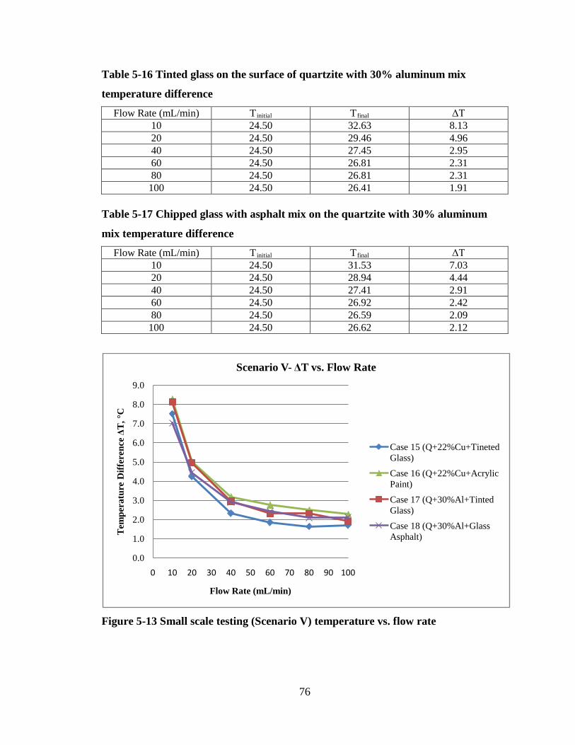
76

Table 5-16 Tinted glass on the surface of quartzite with 30% aluminum mix



Table 5-17 Chipped glass with asphalt mix on the quartzite with 30% aluminum

mix temperature difference


Figure 5-13 Small scale testing (Scenario V) temperature vs. flow rate

0.0

1.0

2.0

3.0

4.0

5.0

6.0

7.0

8.0

9.0

0 10 20 30 40 50 60 70 80 90 100

Tem

pera

ture

Diff

eren

ce Δ

T, °

C

Flow Rate (mL/min)

Scenario V- ΔT vs. Flow Rate

Case 15 (Q+22%Cu+Tineted Glass)

Case 16 (Q+22%Cu+Acrylic Paint)

Case 17 (Q+30%Al+Tinted Glass)

Case 18 (Q+30%Al+Glass Asphalt)

77

Figure 5-14 Small scale testing (Scenario V) temperature difference ΔT

Figure 5-15 Small scale testing (Scenario V) power generated

0.0

1.0

2.0

3.0

4.0

5.0

6.0

7.0

8.0

9.0

10.0

Asphalt Mix

Tem

pera

ture

Diff

eren

ce Δ

T °C

Small Scale Lab Sample Testing

Scenerio V- ΔT at 10mL/min

Case 15 (Q+22%Cu+Tinted Glass)



Case 18 (Q+30%Al+Glass Asphlat)

0.0

1.0

2.0

3.0

4.0

5.0

6.0

Asphalt Mix

Pow

er (W

)

Small Scale Lab Sample s

Scenerio V- Power Generated at 10mL/min


Case16 (Q+22%Cu+Acrylic Paint)



78

Figure 5-16 Effective of Acrylic Paint

The Figure 5-17 showed that the temperature difference (delta T) at 10mL/min for

scenario II, III, IV, and V. The 100% quartzite sample yielded the highest temperature

difference, and 100% RAP was the lowest compared to other samples. Therefore, the

results could be concluded as that the introduced of the quartzite aggregates improved the

overall heat transfer rate for the asphalt pavement.

0.0

1.0

2.0

3.0

4.0

5.0

6.0

7.0

8.0

9.0

0 10 20 30 40 50 60 70 80 90 100

Tem

pera

ture

Diff

eren

ce Δ

T, °

C

Flow Rate (mL/min)

Scenario V- Effective of Acrylic Paint

Case 10 (Q+22%Cu)


79

Figure 5-17 Small scale testing temperature difference ΔT

0.0

1.0

2.0

3.0

4.0

5.0

6.0

7.0

8.0

9.0

10.0

Asphalt Mix

Tem

pera

ture

Diff

eren

ce Δ

T °C

17 Small Scale Lab Sample Testing

Small Scale Testing-ΔT at 10mL/min



Case 9 (100% RAP)

Case 10 (Q+22%Cu)

Case 11 (Q+30%Al)

Case 12 (50%Q+50%RAP)

Case 13 (25%Q+75%RAP)






80

5.5 Robustness Test

The 67% quartzite with 33% limestone mix was selected to be tested it‘s

robustness on randomly testing time. The Figure 5-18 showed that the variability in delta

T from a repeated set of experiments was found to be very low in -0.055 and 0.0916m

location, and sightly higher variation close to the surface. The resutls indicated that the

temperature distribution of asphalt mix was consistily over randomly heating period.

Table 5-18 Repetitive test of 67% quartzite and 33% limestone mix

Apr. 3 Apr. 7 Apr. 9 Apr. 25 Apr. 28 Depth (m) T (°C) T (°C) T (°C) T (°C) T (°C) Avg. STDEV

0 76.54 82.52 81.67 78.49 78.66 79.58 2.46 -0.0254 69.33 73.48 72.08 68.95 68.55 70.48 2.18 -0.055 60.81 61.18 60.51 60.79 60.26 60.71 0.35

-0.0916 55.91 55.61 55.12 56.10 55.34 55.61 0.40

Figure 5-18 5-days repetitive test of 67% quartzite and 33% limestone mix

0

10

20

30

40

50

60

70

80

90

0 60 120 180 240 300 360

Tem

pera

ture

°C

Time (mins)

Quartzite and 33% Limestone Mix Repetition Test (5 Day Average Temperatrue)

0m

-0.0254m

-0.055m

-0.0916m

81


The first set of finite element simulations was carried out to evaluate the effect of

thermal conductivity of the aggregates on the heating process without water flow.

Assuming that the thermal conductivities (k) of the mixtures are primarily influenced by

the conductivity of the aggregates, k values of 5.38 and 2.15 W/m·K (28) were used to

represent quartzite (consisting of mainly quartz) and limestone aggregates (representing

approximately two extremes of thermal conductivity for aggregates) mixes, respectively.

The trial thermal conductivity and heat capacity values were used as seed values

in finite element analysis and compared them with temperature distribution profile from

laboratory data (Appendix D).

The finite element analysis results showed that the quartzite mix had higher

thermal conductivity (Table 5-19) compared to limestone mix and confirmed the

significant effect of thermal conductivity of the HMA on the change in temperature of the

water bath (Figure 5-19) – a delta T of 10.13 and 5.02°C were noted for the quartzite and

the limestone samples, respectively. The model was assumed to be thermally insulated at

every boundary condition excepted for surface of sample. The boundary condition was

assumed to have a heat flux of 1,000W/m2

and convective heat transfer condition. The

mesh size consisted of 32,838 elements and was solved for a time period of 360 minutes.

Table 5-19 Thermal properties of quartzite and limestone sample mix (Appendix D)

Quartzite Limestone Thermal Conductivity (k) 1.8 1.4 Heat Capacity (C) 1050 950 Thermal Diffusivity (α) 7.29e-7 7.61e-7 Lab ΔT 10.13 5.02 FE ΔT 22.77 18.55

The second set of finite element simulations (Figure 5-20) was to evaluate the

effect of thermal conductivity of quartzite and metagranodiorite mixes with various water

flow rates. The model was assumed to be thermally insulated at every boundary

condition excepted for surface of sample, water inlet and water outlet. The boundary

condition was assumed to have a heat flux of 1,000W/m2 and convective heat transfer

condition. The mesh size consisted of 19,165 and was solved for time equaled 60

minutes.

82

Figure 5-19 Steady-state finite element model

Figure 5-20 Transient finite element model

83

The value of the convection heat transfer coefficient for internal flow is dependent

on the geometrical cross section of the pipe, the thermal boundary condition at the pipe

wall, and the distance from pipe entrance.

The Nusselt number is defined as


Where h is the heat transfer coefficient, dh

The Reynolds number, the fluid flow can be characterized into two types of flow

and the velocity profile of the fluid U, can be identified and calculated based on the

Reynolds’s number and Power Law of Velocity (22).

𝑅𝑅𝑒𝑒 =𝜌𝜌𝜌𝜌𝑑𝑑𝜐𝜐

is the hydraulic diameter of the section and k

is the thermal conductivity of the fluid.

Where ρ is the density of the fluid, v is the velocity of fluid, d is the diameter of pipe, and

υ is dynamic viscosity of the fluid.

Laminar flow Re

Turbulent flow R

≤2300


2)

e

Where V

≥2300


7)

max

The fully developed laminar flow was assumed since water flow rate from 10 to

100 ml/min in 0.00675m (1/4”) duct were all laminar flow (Re≤ 2300). The Figure 5-21

and 5-22 showed the temperature distribution along the pipe length from entrance to exit

(y-direction) of both samples, and quartzite mix had lower temperature variation at top

and bottom boundary compared to Wrentham mix. The temperature profile from top to

bottom boundary of pipe (z-direction) (Figure 5-23 and 5-24) indicated that the quartzite

mix had higher heat transfer rate from asphalt to the water, resulting in higher

temperature increased on the center line of the water profile.

is maximum velocity, r is any point at the diameter of pipe, and R is the

radius of the pipe.

84

Figure 5-21 Water temperature distribution along the length of copper pipe

(Quartzite)


(Metagranodiorite)

202224262830323436384042444648505254

-0.075 -0.055 -0.035 -0.015 0.005 0.025 0.045 0.065

Tem

pera

ture

°C

Distance (m)

Quartzite Small Scale Water Temperature 10mL/mim (y-direction) (FE)

Top

Center

Bottom

20222426283032343638404244464850

-0.075 -0.055 -0.035 -0.015 0.005 0.025 0.045 0.065

Tem

pera

ture

°C

Distance (m)

Metagranodiorite Small Scale Water Temperature 10mL/mim (y-direction) (FE)

Top

Center

Bottom

85

Figure 5-23 Water temperature distribution along the depth of copper pipe

(Quartzite)


(Metagranodiorite)

-0.041275-0.040775-0.040275-0.039775-0.039275-0.038775-0.038275-0.037775-0.037275-0.036775-0.036275-0.035775-0.035275

20 22 24 26 28 30 32 34 36 38 40 42 44 46 48 50

Cop

per

Pipe

Dia

met

er (m

)

Temperature °C

Quartzite Small Scale Water Temperature Profile 10mL/min (z-direction) (FE)

Entrance

Center

Exit

-0.041275-0.040775-0.040275-0.039775-0.039275-0.038775-0.038275-0.037775-0.037275-0.036775-0.036275-0.035775-0.035275

20 22 24 26 28 30 32 34 36 38 40 42 44 46 48 50

Cop

per

Pipe

Dia

met

er (m

)

Temperature °C

Metagranodiorite Samll Scale Water Temperature Profile 10mL/min (z-direction) (FE)

Entrance

Center

Exit

86

The finite element analysis results (Table 5-20) showed that the quartzite mix had

higher thermal conductivity compared to metagranodiorite mix and also confirmed the

significant effect of thermal conductivity of the HMA on the change in temperature of the

water outlet.

Table 5-20 Thermal properties of quartzite and metagranodiorite mix (Appendix D)

Quartzite Metagranodiorite Thermal Conductivity (k) 1.8 1.2 Heat Capacity (C) 1050 800 Thermal Diffisivity (α) 7.29e-7 6.38e-7 Lab ΔT (10mL) 8.64 7.52 FE ΔT (10mL) 15.20 13.63

The Figure 5-25 showed that there were 6°C temperature difference between

laboratory and finite element simulations at depth of 0.0381m (1.5”) where was the

location of copper pipe. The both laboratory data did not show the significant effect of

water presented in this location, this can be the indication of that the contact between

asphalt mix and copper pipe were compromised by the drilled hole where allowed copper

pipe to be inserted.

Figure 5-25 Quartzite mix temperature profile

-0.1

-0.09

-0.08

-0.07

-0.06

-0.05

-0.04

-0.03

-0.02

-0.01

0

45 47 49 51 53 55 57 59 61 63 65 67 69

Dep

th (m

)

Temperature °C

Quarzite Small Scale Temperature Profile (Experiment vs FE)

60 mins (LAB)

60 mins (FE)

87

5.7 Discussion

The experiment resuls showed the feasibilties of improving the overall thermal

conducitivty of asphalt pavement by

1. Replacing the conventional aggregate (metagranodiorite) by quartzite

aggregate, which increased the overall thermal conductivity by nearly 50%.

2. Modifying the surface condition of asphalt pavement, such as using acrylic

paint to increased the abosoptivity of pavement.

The asphalt mixes created by using different precentage of materials such as

limestone and copper poweder did not show the increased of water temperature in term of

overall thermal conducitivity. The higher conductive materals could be coated by the

asphalt binder and resulted in lower thermal conductivity.

The water temperature profile in the copper pipe showed that the centerline of

water temperature did not reach steady-state and not reach boundary layer temperature,

which meant that the copper pipe length and surface area were needed to be increased in

order to generate higher water outlet temperature.

The temperature distribution in the asphalt samples did not show the presence of

water at the 1.5 inch location. The air gap could increase the thermal resistance between

the asphalt mix and copper pipe and reduced the heat transfer efficiency.

88

CHAPTER 6

HAND-COMPACTED ASPHALT PAVEMENT TESTING

6.1 Introduction

The results from chapter 5 showed that the major factors that would affect the

heat transfer efficient in the asphalt pavement were surface area of copper pipe, thermal

conductivity of aggregates, percentage of aggregates used in the mix, and contact

between asphalt mix and copper pipe. It was hypothesized that air gap occurred between

asphalt mix and copper pipes because the pipes were installed in the sample after drilling

holes inside the sample which resulting in 6°C difference in sample temperature for

experimental and finite element analysis results. Therefore, in this chapter, the seven

hand-compacted samples were proposed to investigate the effectiveness of increasing

surface area of copper pipe, using different thermal conductivity mix in layers, and

improving contact between asphalt mix and copper pipe.

6.2 Objective


1. Contact between the asphalt mix and the pipe.

2. Different asphalt mix in layers.

3. Pipe layout configurations.

6.3 Methodology

The set of samples (Table 6-1) were compacted and the pipe was placed at the

depth of 0.0381m (Figure 6-1 and 6-2), the compaction procedures are:

1. Prepared one PVC molding (0.1016m (4”) height and 0.1524 (6”) in diameter)

with one base plate.

2. Placed the first layer of asphalt mix, approximately 0.0127m (0.5”) in depth, and

compacted.

3. Positioned one thermocouple on the top center of the first layer.

4. Placed and compacted the second layer of asphalt mix, approximately 0.0381m

(1.5”) in depth.

5. Positioned one thermocouple on the top center of the second layer.

6. Place and compacted the third layer of asphalt mix, approximately 0.0127m (0.5”)

in depth.

89

7. Removed top half of PVC molding and placed 0.00635m (¼”) diameter cooper

pipe on top of third layer. Placed back top half of molding in order to secure the

copper pipe.

8. Placed and compacted the forth layer of asphalt mix, approximately 0.0127m

(0.5”) in depth.

9. Positioned three thermocouples on the top center of forth layer with even spacing

of 0.0381m (1.5”) from the edge.

10. Placed and compacted the fifth layer of asphalt mix, approximately 0.0254m (1”)

in depth.

Table 6-1 Description of compacted samples (Appendix E)

Compacted Sample Description

100% M* 100% Metagranodiorite mix

100% Q* 100% Quartzite mix

50% Q*+50% M* 50% Quartzite on the top and 50% Metagranodiorite on the bottom

35%W*+30%Q*+ 35%M* 35% Metagranodiorite on the top, 30% quartzite in the center layer, and 35% o Metagranodiorite on the bottom

100% M*+ Portland cement 100% Metagranodiorite mix with Portland cement placed around copper pipe

100% Q*+6 rings pipe 100% Quartzite mix with a copper pipe consists six rings

100% Q*+rough surface pipe 100% Quartzite mix with a rough surface copper pipe

M*= Metagranodiorite mix, Q*= Quartzite mix

Each sample was heated up for 6 hours before pumping water; the water flow rate

was set to 10mL/min which showed highest temperature variation (the assumption was

based on previous experiment). The water temperature was collected by thermocouple at

the center of the water collector. The copper pipe with 6 rings was expected to created

larger surface area to increase the heat transfer coefficient, and copper pipe with rough

surface was intended to create a better contact with asphalt mix.

90

Figure 6-1 Copper pipe with 6 rings

Figure 6-2 Placement of thermocouples on top layer

91


The temperature distribution of metagranodiorite sample (Figure 6-3) showed

lower temperature difference (approximately 4°C) at the pipe location (-0.0381m)

compared to earlier dilled samples (approximately 6°C), In addition, the outlet water

temperature was higher; this indicated an importance of the compaction process and the

necessity to ensure maximum contact between the sample and the pipe.

Figure 6-3 Drilled vs. compacted sample temperature distribution

The Table 6-2, 6-3, and Figure 6-4, 6-5 showed the water temperature after 60

minute and 180 minutes of heating, and results showed that the 100% quartzite mix had

better ability to increased water temperature compared to metagranodiorite mix due to its

higher thermal conductivity. In addition, the quartzite mix had higher thermal

conductivity and heat capacity and improved the heat transfer when it was placed

between metagranodiorite mixes.

The Portland cement that was placed surrounding the copper pipe and resulted in

lowest water temperature generated; this was due to its low thermal conductivity and

reduced heat transfer ability from asphalt mix to water.

-0.1

-0.09

-0.08

-0.07

-0.06

-0.05

-0.04

-0.03

-0.02

-0.01

0

40 45 50 55 60 65 70 75

Dep

th (m

)

Temperatrue °C

Metagranodiorite Mix Temperature Distribution (Drilled vs. Compacted)

Drilled

Compacted

92

The quartzite mix with 6 rings of copper pipe generated highest water temperature

compared to other samples, this was due to its large surface area and the position of the

rings were closer to the surface where experienced higher temperature. The quartzite mix

with rough copper surface did not generated higher temperature as expected, which was

due to the rough surface would be resulting in air trapped between uneven surface.

Table 6-2 Temperature difference at time= 60 minutes (Lab Data); water flowing at

10 ml/minute

Case 1st ∆T 2nd ∆T 3rd ∆T Average STDEV 100% M* 9.44 10.05 10.12 9.87 0.37 100% Q* 10.73 12.79 10.12 11.21 1.40 50% Q*+50% M* 8.93 10.74 8.33 9.33 1.26 35%M*+30%Q*+ 35%M* 9.53 11.33 11.91 10.93 1.24 100% W*+ Portland cement 8.33 11.42 10.13 9.96 1.55 100% Q*+6 rings pipe 17.30 15.49 16.10 16.30 0.92 100% Q*+rough surface pipe 9.54 10.74 8.95 9.74 0.91


Figure 6-4 Average water temperature difference at time = 60 minutes

0

2

4

6

8

10

12

14

16

18

Cases

Tem

pera

ture

Diff

eren

ce Δ

T °

C

Hand-Compaction Samples

Average Water Temperature Difference at Time= 60 mins

100% Metagranodiorite Mix

100% Quartzite Mix

50% M and 50% Q

2/3 M and 1/3 Q (center layer)

Quartzite with Portland cement surrounding copper pipe

Quartzite and copper pipe with 6 rings (fins)

Quartzite and copper pipe with rough surface

93

Table 6-3 Temperature difference at time= 180 minutes (Lab Data)

Case 1st ∆T 2nd ∆T 3rd ∆T Average STDEV 100% M* 8.93 9.03 7.72 8.56 0.73 100% Q* 9.54 10.41 9.02 9.65 0.70 50% Q*+50% M* 8.33 9.54 8.24 8.70 0.73 35%M*+30%Q*+ 35%M* 8.33 10.13 9.52 9.33 0.92 100% W*+ Portland cement 7.13 9.53 8.93 8.53 1.25 100% Q*+6 rings pipe 13.72 13.70 12.52 13.32 0.69 100% Q*+rough surface pipe 8.34 8.34 7.75 8.14 0.34



The water temperature at 60 and 180 minutes showed that the asphalt samples

reached steady-state condition (equilibrium), the water temperature was stabilized and the

standard deviation was decreased to within 1°C. The significant difference analysis was

performed and found that there was no significant different when the confidence level

was 95%

0

2

4

6

8

10

12

14

Cases

Tem

pera

ture

Diff

eren

ce Δ

T °

C

Hand-Compaction Samples


100% Metagranodiorite Mix

100% Quartzite Mix

50% M and 50% Q

2/3 M and 1/3 Q (center layer)

Quartzite with Portland cement surrounding copper pipe

Quartzite and copper pipe with 6 rings (fins)

Quartzite and copper pipe with rough surface

94


The finite element analysis was used to validate the assumptions and laboratory

data, with the initial temperatures of the three layers as designated by the three

thermocouples after 6 hours as input. The thermal conductivity and heat capacity were

back-calculated based on 6 hours heating period of metagranodiorite and quartzite to

verify if there was difference between gyrator compaction and hand compaction

(Appendix F).

Table 6-4 and 6-5 showed that the thermal properties were not affected

significantly when two different compaction methods were used. The thermal diffusivity

of hand-compacted quartzite mix was increased than gyrator compacted, and was

decreased in metagranodiorite mix.

Table 6-4 Quartzite mix back-calculated thermal properties

Gyrator Compacted Hand-Compacted Thermal Conductivity (k) 1.8 2.0 Heat Capacity (C) 1050 950 Thermal Diffusivity (α) 7.29e-7 8.9e-7

Table 6-5 Metagranodiorite mix back-calculated thermal properties

Gyrator Compacted Hand-Compacted Thermal Conductivity (k) 1.2 1.1 Heat Capacity (C) 800 900 Thermal Diffusivity (α) 6.38e-7 5.2e-7

95

The results of finite element analysis (Table 6-6) showed that the water

temperature of copper pipe with 6 rings generated highest temperature compared to the

others.

Table 6-6 Laboratory and finite element analysis temperature difference at time =

60 minutes comparison

Case Lab ∆T °C FE ∆T °C 100% M* 9.87 13.91 100% Q* 11.21 15.91 50% Q*+50% M* 9.33 18.62 35%M*+30%Q*+ 35%M* 10.93 16.2 100% M*+ Portland cement 9.96 6.87 100% Q*+6 rings pipe 16.30 19.34 100% Q*+rough surface pipe 9.74 17.8


Table 6-7 Laboratory and Finite Element temperature difference at time = 180

minutes comparison

Case Lab ∆T °C FE ∆T °C 100% M* 8.56 12.89 100% Q* 9.65 14.91 50% Q*+50% M* 8.70 15.4 35%M*+30%Q*+ 35%M* 9.33 14.56 100% M*+ Portland cement 8.53 6.9 100% Q*+6 rings pipe 13.32 13.22 100% Q*+rough surface pipe 8.14 15.51


The finite element analysis results (Table 6-7) showed higher temperature

compared to laboratory results because in finite element model, the asphalt sample was

assumed to be homogenous material, and perfect contact with the copper pipe. However,

the asphalt sample was mixed with different size of aggregate and asphalt binder, each of

components has different thermal properties and affect heat transfer rate.

96

6.6 Discussion

Improving the contact between the asphalt mix and copper pipe showed the

evidence of increasing of water temperature (outlet) by 2.57°C for quartzite mix and 2.35

°C for metagranodiorite mix in 60 minute period when compared to small scale testing.

The 35% metagranodiorite on top layer, 30% quartzite in the center layer, and

35% metagranodiorite on the bottom layer showed the higher temperature difference in

Finite Element results, which showed that the lower heat capacity (metagranodiorite) on

the top layer was heated up faster to increase the heat transfer rate for the higher thermal

conductivity (quartzite) in the center layer.

The water temperature never reached the asphalt sample temperature at 1.5 inch

below the surface could be an indication of insufficient surface area of copper pipe. The

experiment results showed that the increased of surface area and the location of pipe

placement could greatly increase the outlet water temperature. Therefore, the analytical

approach for effective pipe length, diameter, and water flow rate must be performed.

97

CHAPTER 7

DETERMINE EFFECTIVE PIPE LENGTH AND SPACING

7.1 Introdution

The experimental results showed that the maximum average temperature below

0.0254m (1”) of the asphalt pavement surface was approximately 50 °C. The value was

then used as uniform wall temperature to determine the effective copper pipe length, pipe

diameter, and water flow rate by using analytical approach. The chart of the effective

copper pipe length, diameter versus water flow rate was developed. The laboratory

experiemnts were perfomed to validated the effect of pipe legth and configuration in term

of difference at water outlet temperature.

7.2 Objective


1. Effect of pipe length

2. Effect of pipe diameter

3. Effect of pipe spacing

4. Effect of water flow rate

5. Effect of pipe layout configuration

7.3 Methodology

The value of the convection heat transfer coefficient for internal flow is dependent

on the geometrical cross section of the duct, the thermal boundary condition at the pipe

wall, and the distance from pipe entrance. The Nusselt number is defined as


Where dh

There are two types of boundary conditions used in convection heat transfer,

uniform wall flux and uniform wall temperature.

is the hydraulic diameter of the section and k is the thermal conductivity of the

fluid, h is the heat transfer coefficient.

Uniform wall flux �̇�𝑞𝑤𝑤" is when the heat flux at the wall of the duct is uniform,

98

𝑇𝑇𝑏𝑏 =�̇�𝑞𝑤𝑤" 𝐴𝐴�̇�𝑚𝐶𝐶𝑝𝑝

+ 𝑇𝑇𝑖𝑖

�̇�𝑞𝑤𝑤" = ℎ𝑥𝑥(𝑇𝑇𝑤𝑤 − 𝑇𝑇𝑏𝑏)

Where Tb is the exit temperature, A is the surface area of the duct, �̇�𝑚 is the mass flow

rare, Cp is heat capacity, Ti is the initial temperature at the entrance, hx is the local heat

transfer coefficient, and Tw

Uniform wall temperature is when the temperature at the wall is uniform; the

local heat flux is replaced by ℎ𝑥𝑥(𝑇𝑇𝑤𝑤 − 𝑇𝑇𝑏𝑏), the equation can be rearranged as (21)

𝑇𝑇𝑤𝑤 − 𝑇𝑇𝑏𝑏𝑇𝑇𝑤𝑤 − 𝑇𝑇𝑖𝑖

= 𝑒𝑒𝑥𝑥𝑝𝑝 �−ℎ�𝐴𝐴�̇�𝑚𝐶𝐶𝑝𝑝

�

is the wall temperature.

Where ℎ� is the average heat transfer coefficient.

Table 7-1 The typical Nusselt number for fully developed flow

Uniform Heat Flux Uniform Wall Temperature Circular Duct 4.36 3.66

Table 7-2 Calculated required pipe length at wall temperature= 50 °C

Water Flow Rate (mL/min)

Pipe Diameter (m) 100 200 400 600 800 1000 2000 4000 6000 8000 10000 0.005 7.5 15 30 45 60 75 150 300 450 600 750 0.01 7.5 15 30 45 60 75 150 300 450 600 750 0.02 7.5 15 30 45 60 75 150 300 450 600 750 0.03 7.5 15 30 45 60 75 150 300 450 600 750 0.04 7.5 15 30 45 60 75 150 300 450 600 750 0.05 7.5 15 30 45 60 75 150 300 450 600 750 0.06 7.5 15 30 45 60 75 150 300 450 600 750 0.07 7.5 15 30 45 60 75 150 300 450 600 750 0.08 7.5 15 30 45 60 75 150 300 450 600 750 0.09 7.5 15 30 45 60 75 150 300 450 600 750 0.1 7.5 15 30 45 60 75 150 300 450 600 750

Pipe length (m)

*highlight is where turbulent flow occurs

99

The heat transfer coefficient was inversed to the hydraulic diameter (wet

perimeter of pipe diameter), therefore, the smaller diameter of pipe resulted in highest

heat transfer coefficient and required shorter length to achieve the 50°C wall temperature.

In contrast, the larger diameter of copper pipe required longer length (Figure 7-1).

Figure 7-1 Effective pipe diameter, length, and flow rate chart

1

10

100

1000

10000

1 10 100 1000

Wat

er F

low

Rat

e (m

L/m

in)

Pipe Length (m)

Effective Pipe Diameter, Pipe Length, and Flow Rate ChartWall Temperature = 50 °C

D=0.005m

D=0.01m

D=0.02m

D=0.03m

D=0.04m

D=0.05m

D=0.06m

D=0.07m

D=0.08m

D=0.09m

D=0.1m

100


Since the actual length of pipe is limited, and it cannot be provided as a straight

section, therefore, 3 different pipe layouts (1) 0.1524m (6”) straight pipe, (2) 0.3556m

(14”) serpentine style pipe, and (3) 0.7112 (28”) serpentine style pipe (Figure 7-2) were

proposed to validate the theoretical approach. The same compaction procedures were

used as Charter 6. Each sample was heated up for 6 hours before pumping water; the

water flow rate was set to 10mL/min which showed highest temperature variation (the

assumption was based on previous experiment). The water temperature was collected by

thermocouple at the center of the water collector.

Figure 7-2 Serpentine pipe being placed and compacted

101

Table 7-3 Average water temperature difference at time= 60 minutes

Case 1st ∆T 2nd ∆T 3rd ∆T Average STDEV 6" Straight Pipe 10.73 12.79 10.12 11.21 1.40 14" Serpentine Pipe 21.75 18.79 19.76 20.10 1.51 28" Serpentine Pipe 25.13 20.85 22.89 22.89 2.15


0

5

10

15

20

25

Cases

Tem

pera

ture

Diff

eren

ce Δ

T °

C

Hand Compaction Samples


6in Straight pipe

14in Serpentine pipe


102

Table 7-4 Average water temperature difference at time= 180 minutes

Case 1st ∆T 2nd ∆T 3rd ∆T Average STDEV 6" Straight Pipe 9.54 10.41 9.02 9.65 0.70 14" Serpentine Pipe 17.49 15.07 16.15 16.24 1.21 28" Serpentine Pipe 21.22 17.81 18.05 19.03 1.90


The experiment results showed that the pipe with larger surface area yielded

higher temperature at the water exit. When the pipe length increased from 0.1524m (6”)

to 0.3556m (14”), the temperature resulted in approximately 8.55°C difference, when the

pipe length increased from 0.3556m (14”) to 0.7112m (28”), the temperature only

increased approximately 7.37°C, which meant that the large surface area of pipe yielded

higher temperature.

0

2

4

6

8

10

12

14

16

18

20

Cases

Tem

pera

ture

Diff

eren

ce Δ

T °

C

Hand Compaction Samples


6in Straignt pipe



103

7.5 Finite Element Analsis/Modeling

Based on the analytical results, the copper length and diameter ratio was very

large (>5000), and finite element analysis approach was unable to model in 3D

simulation, therefore, the finite element was used to determine the effective pipe spacing

and investigated where the lowest temperature zone occurred between different pipe

spacing because finite element analysis simulated the heat transfer interaction between

asphalt pavement and water, and the lowest temperature zone meant that the asphalt

pavement temperature would be very close to water temperature, and the convective heat

transfer of water would not be affected by another water domain. The asphalt pavement

temperature was assumed to be constant temperature 50°C, water temperature was

constant 25°C, and the various pipe diameters were analyzed by using the pipe spacing

from 0.0254m (2”) to 0.6096m (24”).

Figure 7-5 Temperature variation between two pipes

Note that the smaller hydralic diameter resulted in lower termperature variation

between the pipes, when the pipe spacing were equal to 0.3556m (14”) and 0.4064m

(16”), - the temperature variation was minimal because the convective heat transfer

coefficient was greater and the temperature drop between pipes was increased (as asphlat

30

32

34

36

38

40

42

44

46

48

50

0.0 0.2 0.4 0.6 0.8 1.0 1.2 1.4 1.6 1.8 2.0

Tem

pera

ture

°C

Pipe Spacing (m)

Temperature Between Two Pipes (FE) 4000mL/min

D=0.005m

D=0.01m

D=0.02m

D=0.03m

D=0.04m

104

pavement temperature = 50°C). On the other hand, the convective heat transfer

coefficient was decreased when the flow rates increased and this resulted in lower

temeprature drop between two pipes.

Figure 7-6 Finite element model for temeprature variation between various pipe

spacing

Three serpentine pipe layouts were analyzed by assuming the boundary

conditions to a constant temperature (based on lab data) along the interface with asphalt

sample and others are thermally insulated, and 10mL/min water flow rate (fully

developed laminar flow) was used as water velocity; in actual experiment the temperature

of the pipe will not be constant along the diameter of the sample, since because of the

cold water entering, the pipe part near the inlet will be at a lower temperature than the

remaining part; this could at least partially explain the difference between finite element

analysis (higher) and the lab delta Ts.

The results of the finite element analysis (Figure 7-7 to 7-9) clearly showed the

higher temperature of the water for the serpentine pipes as compared to the straight pipe.

105

Figure 7-7 Straight pipe 0.1524m (6”) (temperature distribution)

Figure 7-8 Serpentine pipe 0.3556m (14”) (temperature distribution)

106

Figure 7-9 Serpentine pipe 0.7112m (28”) (temperature distribution)

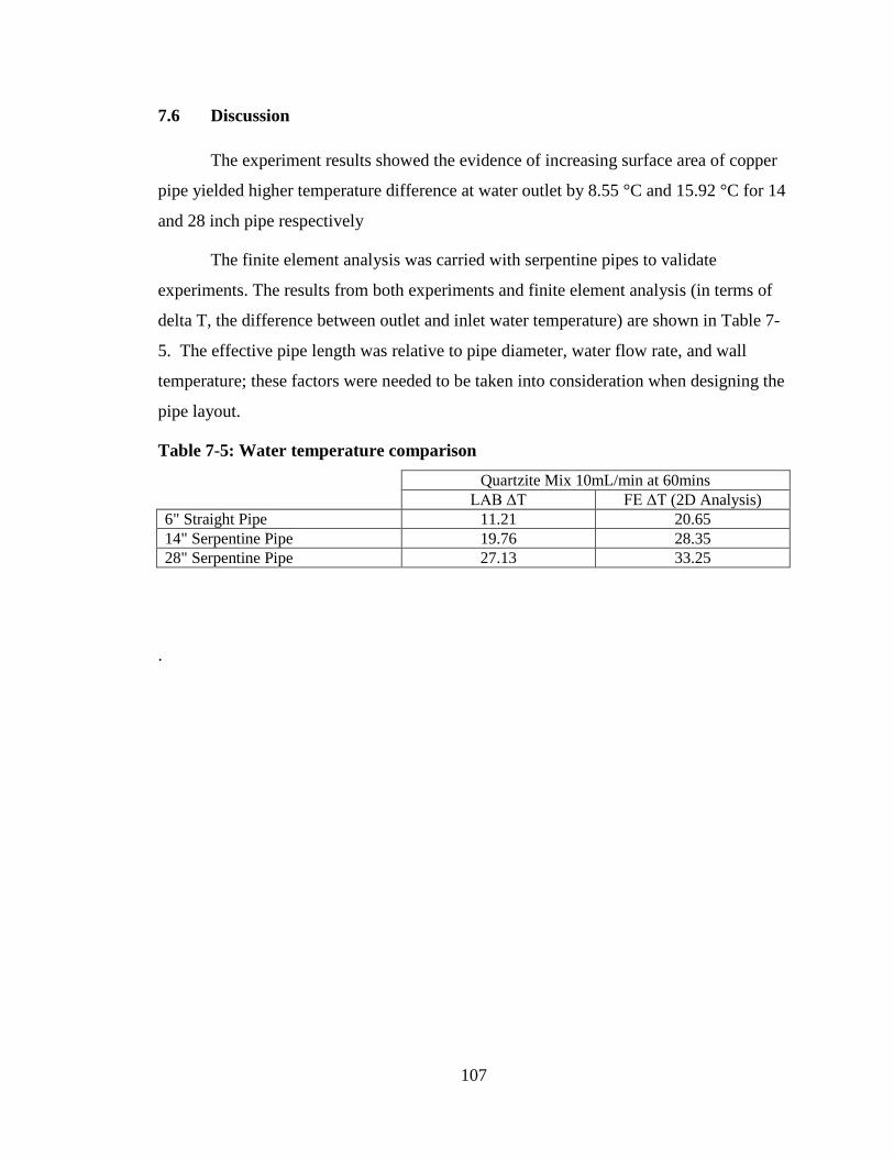
107

7.6 Discussion

The experiment results showed the evidence of increasing surface area of copper

pipe yielded higher temperature difference at water outlet by 8.55 °C and 15.92 °C for 14

and 28 inch pipe respectively

The finite element analysis was carried with serpentine pipes to validate

experiments. The results from both experiments and finite element analysis (in terms of

delta T, the difference between outlet and inlet water temperature) are shown in Table 7-

5. The effective pipe length was relative to pipe diameter, water flow rate, and wall

temperature; these factors were needed to be taken into consideration when designing the

pipe layout.

Table 7-5: Water temperature comparison

Quartzite Mix 10mL/min at 60mins

LAB ΔT FE ΔT (2D Analysis) 6" Straight Pipe 11.21 20.65 14" Serpentine Pipe 19.76 28.35 28" Serpentine Pipe 27.13 33.25

.

108

CHAPTER 8

REDUCE URBAN HEAT-ISLAND EFFECT

8.1 Introduction

Asphalt pavements get heated up by solar radiation, and numerous studies have

been conducted on evaluation of temperature profiles inside asphalt pavements, and the

effect of different parameters on such temperature. Because surface radiation follows the

Stefan-Boltzmann equation, which involves the fourth power of temperature, a slight

increase in the surface temperature results in a significant increase in the emitted heat.

This leads to significant increase in energy consumption in order to maintain comfort

level. Additionally, studies have shown that air quality also deteriorates under increased

temperature due to the Urban Heat-Island Effect.

The hypothesis of this chapter is that the surface temperature of the asphalt

pavement will be reduced due to the convective heat transfer of water flowing underneath

it, which will decrease the back radiated energy emitted from asphalt pavement to the air.

8.2 Objective

The objectives of this chapter were to evaluate

1. The effect of the surface temperature of asphalt pavement based on different

thermal conductivity of mix.

2. The effect of the surface temperature of asphalt pavement based on different

surface area of copper pipe.

8.3 Methodology

The transfer of energy by electromagnetic waves is called radiation heat transfer.

All matter at temperature greater than absolute zero will radiate energy. Energy can be

transferred by thermal radiation between a gas and solid surface or between two or more

surface. The rate of energy emitted by an ideal surface (black body) with emissivity

equal to 1 is given by the Stefan-Boltzmann law (20):

109

4sb TE εσ=

Where Eb is the rate of black body radiation energy, ε is the emissivity of the material,

and σ = Stefan-Boltzmann constant = 5.68x10-8 W/(m2K4), and Ts

The emitted radiation intensity from the pavement surface to its surroundings is

calculated as:

is surface temperature,

K.

)( 44airsr TTq −= εσ

Where qr = emitted radiation, h is heat transfer coefficient, ε is the emissivity of the

material, σ = Stefan-Boltzmann constant = 5.68x10-8 W/(m2∙K4), Ts is surface

temperature in Kelvin, Tair

The emissivity of a material ε is the ratio of energy radiated by the material to

energy radiated by a black body at the same temperature. It is a measure of a material's

ability to absorb and radiate energy. A true black body would have the value of ε = 1

while any real object would have ε < 1. Emissivity depends on factors such as

temperature, emission angle, and wavelength. Based on Stefan- Boltzmann law, the

variable that would reduce the back-radiated energy is the temperature difference

between the asphalt pavement surface and ambient temperature (air).

is air temperature Kelvin.

110


In the first step, three thermocouples were used for the temperature data collection

from the surface one directly at the center, and other two 0.0254m (1”) from the sample

edge (Figure 8-1). This arrangement was made for four samples – two for quartzite mix

and two for metagranodiorite mix. The samples were compacted in similar manner, using

the same amount of asphalt binder. (Bulk specific gravity for Q mix= 2.208 and M mix=

2.265). Of the two samples made for each mix, one was fitted with a copper pipe

approximately 1.5 inch below the surface to flow water through it.

Figure 8-1 Samples with three thermocouples

150mm Diameter

T1

T3

T2

38.1 mm

38.1 m

m

T1, T2, T3- surface

102

mm

¼”Copper Tube

100% Quartzite

111

For the samples without pipe, the lamp was left on for eight hours, and then

switched off, and data were collected for the next eight hours; this procedure was

repeated three times for each sample with 24 hours interval between two successive

heating cycles.

For the sample with pipe, the lamp was left on for four hours, without flowing

water, and water was flowed for four hours after which the lamp was switched off and the

water was kept flowing for another four hours. This procedure was repeated three times

for each sample with 24 hours interval between two successive heating cycles.

Plots of surface temperature versus time are shown in Figures 8-2 and 8-3. Figure

8-2 showed that the maximum temperature of the metagranodiorite mix is higher than the

maximum temperature of the quartzite mix. This is due to the higher thermal conductivity

of the quartzite mix. Figure 8-3, in comparison to Figure 8-2, showed clearly that the

maximum temperatures reached in the two samples with water flow were significantly

lower compared to those without any water flow.

Figure 8-2 Quartzite and metagranodiorite mixes for 8 hour heating and 8 hour no

heating data for surface temperature (T2 thermocouple)

0

10

20

30

40

50

60

70

80

90

100

0 120 240 360 480 600 720 840 960

Tem

pera

ture

°C

Time (mins)

Quartzite and Metagranodiorite Mix Heating and Cooling(16 hours) T2 Temperature

Quartzite Mix

Metagranodiorite Mix

T2

112

Figure 8-3 Heating with water flow data for surface temperature (T2 thermocouple)

for quartzite and metagranodiorite Mixes.

0

10

20

30

40

50

60

70

80

90

100

0 120 240 360 480 600 720

Tem

pera

ture

°C

Time (mins)

Quartzite and Metagranodiorite Mix Heating and Cooling(12 hours) T2 Temperature

Quartzite Mix


T2

113

In the next step, a detailed investigation of the quartzite samples only was

conducted, using seven thermocouples for each sample, as shown in Figure 7-4 and 7-5.

Figure 8-4 Schematic of thermocouple locations on the surface of asphalt sample

Figure 8-5 Thermocouple locations on the surface of asphalt sample

150 Di

T1

T6

T5

T4

T3

T2

38.1 mm

38.1 m

m

T7

114

The following plots (Figure 8-6 to 8-12) showed the temperature versus time data

for each of the seven thermocouples (T1 through T7) on the surface, for the case where

the sample was heated for 8 hours and then not heated for the next 8 hours (designated as

8/8 hrs), and the case for which the sample was heated for 8 hours, where water was

flowed after the first 4 hours of heating and then not heated for 4 hours (designated as

4/4/4 hrs).

All of the plots, except the one for the T7 thermocouple, showed that there was a

significant reduction in surface temperature of the sample as a result of flowing water.

They also showed that at the end of the heating period, the cooling rate was higher for the

samples that have water flowing through them.

The results were more prominent for the T1, T2 and T3 thermocouples, which

were at the center line of the sample and fell immediately above the copper pipe carrying

water inside the sample.

Figure 8-6 Plots of time versus temperature (T1)

0

10

20

30

40

50

60

70

80

90

100

0 120 240 360 480 600 720 840 960

Tem

pera

ture

°C

Time (mins)

Quartzite Mix Heating and Cooling T1 Temperature

Quartzite Mix (8/8 hrs)

Quartzite Mix (4/4/4 hrs)

T1

115



0

10

20

30

40

50

60

70

80

90

100

0 120 240 360 480 600 720 840 960

Tem

pera

ture

°C

Time (mins)




T2

0

10

20

30

40

50

60

70

80

90

100

0 120 240 360 480 600 720 840 960

Tem

pera

ture

°C

Time (mins)




T3

116



0

10

20

30

40

50

60

70

80

90

100

0 120 240 360 480 600 720 840 960

Tem

pera

ture

°C

Time (mins)




T4

0

10

20

30

40

50

60

70

80

90

100

0 120 240 360 480 600 720 840 960

Tem

pera

ture

°C

Time (mins)




T5

117



0

10

20

30

40

50

60

70

80

90

100

0 120 240 360 480 600 720 840 960

Tem

pera

ture

°C

Time (mins)




T6

0

10

20

30

40

50

60

70

80

90

100

0 120 240 360 480 600 720 840 960

Tem

pera

ture

°C

Time (mins)




T7

118

The filament of the halogen lamp operated at very high temperature and delivers a

“cone” heat flux onto sample surface. The thermocouples on the sample surface were

very sensitive to the position of the halogen lamp; this caused slightly different

temperature measurement (as shown for T7). Table 8-1 showed the average reduction of

temperature for the different locations on the sample.

Table 8-1 Average reduction in surface temperature due to flowing water

Thermocouple T1 T2 T3 T4 T5 T6 T7 Max 70.83 76.77 61.30 66.98 64.31 61.71 57.12 Min 57.40 72.09 56.33 57.32 58.94 55.69 55.10

ΔT (°C) 13.43 4.68 4.96 9.65 5.37 6.02 2.02 Note: The position of T2 is right underneath the halogen filament and the measured temperature is always slightly higher From the various plots in Figure 8-14 to 8-20, it can be seen that for the first 4

hours all thermocouples showed similar rise in temperature; however when water was

turned on thermocouples T1-T6 show lower temperature over the next four hours. The

mean drop on temperature (ΔT) was 13.43°C for T1 because its location is near the pipe

(water) entrance region which had the coldest water (25.5°C) that led to the largest drop

in temp. The effect seems to taper off in the midsection by T2 and also in the tail-end

section (T3).

The other prominent effect was the significant lowering of temperature at T4

which is placed 38.1mm from the centerline of the pipe. The temperature at this location

fell by almost 10°C. The numbers steadied to between 5 and 6°C in the midsection at

these far locations (38.1mm). Results indicate that the cooling potential of water flowing

through a pipe can radially extend for almost 40mm.

To evaluate the effect of increased surface area of pipe on the drop in

temperature, experiments were conducted with pipes of serpentine (S) shape (Figure 8-

13), so as to cover more area of the HMA sample. The plots for the experimentally

obtained data for the 28 inch serpentine pipe for T1-T7 are shown in Figure 8-14 to 8-20.

The results clearly show the higher reduction of surface temperature for the

serpentine pipes compared to the straight pipe.

119

Figure 8-13 Serpentine pipe in a sample (during compaction)


0

10

20

30

40

50

60

70

80

90

100

0 120 240 360 480 600 720

Tem

pera

ture

°C

Time (mins)


Straight (4/4/4 hrs)

Serpentine (4/4/4 hrs)

T1

120



0

10

20

30

40

50

60

70

80

90

100

0 120 240 360 480 600 720

Tem

pera

ture

°C

Time (mins)




0

10

20

30

40

50

60

70

80

90

100

0 120 240 360 480 600 720

Tem

pera

ture

°C

Time (mins)




T2

T3

121



0

10

20

30

40

50

60

70

80

90

100

0 120 240 360 480 600 720

Tem

pera

ture

°C

Time (mins)




0

10

20

30

40

50

60

70

80

90

100

0 120 240 360 480 600 720

Tem

pera

ture

°C

Time (mins)




T4

T5

122



0

10

20

30

40

50

60

70

80

90

100

0 120 240 360 480 600 720

Tem

pera

ture

°C

Time (mins)




0

10

20

30

40

50

60

70

80

90

100

0 120 240 360 480 600 720

Tem

pera

ture

°C

Time (mins)




T6

T7

123

7.5 Discussion

The experiment results of 8 hours heating and 8 hours cooling of quartzite and

metagranodiorite mixes showed that the surface temperature of higher thermal

conductivity of quartzite mix was lower than the metagranodiorite by approximately 4°C.

The experiment results of heating and cooling with water flowing showed that the

surface temperature of quartzite mix was not heated up rapidly and was 7°C lower than

metagranodiorite mix.

The results of seven thermocouples on quartzite mix measurement showed that

the T1 (water inlet) yielded highest surface temperature difference, approximately

13.5°C, which was due to the greater heat transfer coefficient of water flow at water inlet.

Quartzite mix (higher thermal conductivity) with greater surface area of copper

pipe showed the evidence of reducing Heat Island Effect by decreasing the surface

temperature and reduced back-radiated energy emitted to air.

124

CHAPTER 9

LARGE SCALE ASPHALT PAVEMENT TESTING

9.1 Introduction

In this chapter, tests were carried out with large scale slabs. Two slabs were

prepared – each with approximately 125 mm thick HMA layer, with a frame of copper

pipes (Appendix E) embedded inside. The copper pipes were provided for pumping water

(heat exchanger) through the slab. Thermocouples were inserted along the depth and at

various points in the slabs, including points in line with the copper pipe locations, and

inlet and outlet points of the water flowing through the copper pipes.

Two types of materials were used for preparing mixes for the two slabs. The

entire 125mm thickness of the first slab was prepared with a metagranodiorite mix

obtained from a local HMA plant (using aggregates identified as greywacke, with quartz

and feldspar), whereas the second slab was prepared with the local mix for the bottom

64mm, and quartzite aggregate mix (prepared in the laboratory) in the middle and the top

layers. Mixes with both aggregates were made with the same gradation and asphalt

content. Copper pipe frames with multiple pipes along the width and one pipe along the

length were placed approximately 38mm below the surface in both slabs, during

placement and compaction inside wood carts.

The schematics of the two slabs, with copper pipe frame as well as thermocouple

locations are shown in Figure 9-1 to 9-4.

9.2 Objective


1. Temperature distribution of asphalt pavement based on partial replacement of

granite aggregate with quartzite, and performing different water flow rate and

pipe opening combinations.

2. The effect of heat exchanger system to pavement temperature and validate the

previous laboratory experiments.

125

Figure 9-1 Schematics of slab with thermocouple, copper pipes, and water flow

direction

Figure 9-2 Dimension of slab and copper frame

Copper pipes

1.5’

1.5’

6’

1.5’ 1.5’ 1.5’ 1.5’

Slab Plan View

3’

Wood cart with thermocouples at the inside bottom

125 mm thick slab with thermocouples at five points along depth – surface, 22 mm, 35 mm, 86 mm, 119

Orange lines indicate copper tubes and red lines indicate thermocouples

Blue arrows indicate flow of water

126

Figure 9-3 Metagranodiorite mix slab thermocouple location

Figure 9-4 Quartzite mix slab thermocouple location

0.9”

0.5”

1.5”

0.5”

1.3”

4.7”

1

2

3

4

5

6

7

8

9

10

11

12 13

14 15 16

Quartzite Mix

6‘

0.5”

0.5”

1.5”

0.5”

2.31”

5.31”

MetagranodioriteMix

1

2

3

4

5

6

7

8

9

10

11

12 13

14 15 16

6‘

127

9.2 Objective


1. Effect of temperature distribution of asphalt pavement based on partial

replacement of metagranodiorite aggregate with quartzite.

2. Effect of temperature distribution of asphalt pavement by performing different

water flow rate and pipe opening combinations.

3. Effect of convective heat transfer at surface of asphalt pavement.

4. Feasibility of reduce Urban Heat-Island Effect by inserting heat exchanger system

underneath of asphalt pavement.

9.3 Methodology

Temperature data was first collected for both slabs without flow any water. The

data received from the thermocouples (Figure 9-3 and 9-4) inserted at various points were

used to determine the temperature profile within the slabs.

Next, a hose was connected from the same water supply to pump water through

the copper tubes in both slabs at the same rate. First, before flowing any water, the slabs

were kept under the sun for approximately two hours, and temperatures at the various

depths at the center of the slabs were recorded. Next, water was pumped at 1, 2, 3 and

4L/min through both slabs with different pipe opening combinations, and temperature of

the slab at the middle copper pipe location as well as incoming and outgoing water were

measured (Figure 9-5).

128

Figure 9-5 Two slabs tests under the field conditions

129


Figure 9-6 and 9-7 illustrated both slabs temperature profiles over time at

different depths over a period of 5 hours and under an average of 716W/m2

solar

radiation. As clearly indicated by the temperature profiles of thermocouples placed with

increasing depth, temperature was a function of depth, with thermocouples placed closer

to the surface recording higher temperature at any instant of time. This process was

consistent through all the reading and progressive depths. However, an important

observation from these sets of graphs was that the time at which steady state was reached

at different depths vary.

Figure 9-6 Metagranodiorite mix slab temperature profile

0

10

20

30

40

50

60

0 60 120 180 240 300 360

Tem

pera

ture

°C

Time (min)

Metagranodiorite Slab Temperature Profile

T15

T8

T7

T6

T5

130

Figure 9-7 Quartzite mix slab temperature profile

At 0.0127m (T8) depth of metagranodiorite slab, steady state was reached quickly

(the scatter in the data induced by solar radiation fluctuation and wind velocities made the

exact prediction impossible). At 0.0254m of metagranodiorite slab, the steady state was

reached in 300 minutes, and quartzite slab showed much faster heating rate when it

reached steady state at 60 to 120 minutes. The lowest 2 thermocouples (T5 and T6) of

metagranodiorite slab reached steady state at the end of the 360 hours period, and

quartzite slab reached at 300 minutes. The temperature profile of two slab showed that

the quartzite slab had higher heating rate compared to metagranodiorite, this was also the

indication of the higher thermal conductivity of quartzite slab opposed to

metagranodiorite slab.

The results indicated that the depth (0.0381m) at which the pipes were placed was

clearly important for a temperature profile like this as seen from the graphs. At a

hypothetical depth of 0.0254m, the steady state temperature of approximately 50°C can

be obtained for heating pipes whereas at 0.0254m the temperature was 50°C and transient

for a longer period.

0

10

20

30

40

50

60

0 60 120 180 240 300 360

Tem

pera

ture

°C

Time (min)

Quartzite Slab Temperature Profile

T15

T8

T7

T6

T5

131

The both slabs were tested with 4 difference flow rates (1, 2, 3, 4L/min) and all

copper pipes running water. The water temperature was taken at 3 and 6ft of copper pipe.

The Figure 8-8 showed the typical thermocouple locations for collecting temperature

data.

Figure 9-8 Metagranodiorite slab thermocouple locations

Table 9-1 and Figure 9-9 showed that, with increasing flow rate the temperature

raised of water flowing through a pipe are reduced. The temperature rise was generally

more for the longer tube because of the higher area of heat transfer available due to the

longer length. This translated into more power being extracted by flowing the water

through a longer pipe. The results also showed that the quartzite slab which had higher

thermal conductivity can yield higher temperature at the water outlet.

5

4

3

6

7

2

1

8

0.5”

0.5”

1.5”

0.5”

2.31”

5.31”


6’

132

Table 9-1 Metagranodiorite slab water temperature (all pipe open)

Tinitial T (°C) final ΔT (°C) (°C)

1L/min (3') 22.98 24.52 1.54 2L/min (3') 22.72 23.71 0.99 3L/min (3') 22.73 23.22 0.49 4L/min (3') 22.74 23.59 0.85 1L/min (6') 22.98 24.61 1.63 2L/min (6') 22.72 24.56 1.84 3L/min (6') 22.73 24.03 1.30 4L/min (6') 22.74 23.87 1.13

Figure 9-9 Water temperature measured at 3ft pipe outlet for both slabs

0.0

0.5

1.0

1.5

2.0

2.5

0 1 2 3 4 5

Tem

pera

ture

Diff

eren

ce Δ

T,

°C

Flow Rate (L/min)

Slab Test Water Temperature at 3ft Pipe with All Pipes Open

Metagranodiorite

Quartzite

133

Table 9-2 Quartzite slab water temperature (all pipe open)

Tinitial T (°C) final ΔT (°C) (°C)

1L/min (3') 22.98 25.20 2.22 2L/min (3') 22.72 23.25 0.53 3L/min (3') 22.73 24.00 1.27 4L/min (3') 22.74 23.59 0.85 1L/min (6') 22.98 25.47 2.49 2L/min (6') 22.72 23.37 0.65 3L/min (6') 22.73 24.16 1.43 4L/min (6') 22.74 23.62 0.88

Figure 9-10 Water temperature measured at 6ft pipe outlet for both slabs

The results (Table 9-2 and Figure 9-10) indicated the beneficial effect of having

heat exchangers with a large surface area exposed to the pavement for extraction of heat.

A comparison between quartzite and metagranodiorite mix slabs showed that the

temperature difference from the quartzite pavement was higher for flow rate of 1 and

3L/min, whereas the metagranodiorite slab showed higher temperature for the long pipe

at 4 L/min.

The quartzite slab was then tested with four water flow rates with only one 3ft

long copper pipe, and 1L/min for two 3ft long copper pipes to obtain the temperature

0.0

0.5

1.0

1.5

2.0

2.5

3.0

0 1 2 3 4 5

Tem

pera

ture

Diff

eren

ce Δ

T, °

C

Flow Rate (L/min)

Slab Test Water Temperature at 6ft Pipe with All Pipes Open

Metagranodiorite

Quartzite

134

profile as well as effect of flow rate and copper pipe spacing (Table 9-3 to 9- 6, and

Figure 9-11 to 9- 14).

Table 9-3 Quartzite slab temperature profile with 1L/min (1 pipe)

Time (min) -0.11938m -0.08636m -0.03556m -0.02286m 0m 0 37.23 40.38 50.15 50.95 50.64

10 37.46 37.11 46.85 49.47 49.69 20 36.76 36.88 48.56 49.24 48.27 30 36.30 36.06 47.64 47.87 48.52 35 37.50 37.48 48.68 48.79 47.73

Figure 8-11 Quartzite mix slab temperature profile (1L/min)

-0.12

-0.1

-0.08

-0.06

-0.04

-0.02

0

30 35 40 45 50 55

Dep

th (m

)

Temperature °C

Quartzite Slab Temperature Profile 1L/min

0 min

10mins

20 mins

30 mins

35 mins

135


Time (min) -0.11938m -0.08636m -0.03556m -0.02286m 0m 0 37.50 37.48 48.68 48.79 47.73

10 36.22 35.86 46.41 47.20 47.39 20 36.31 35.25 46.39 46.50 47.25 30 35.86 34.91 45.94 46.17 47.39 35 36.36 35.05 46.19 46.30 46.46


-0.12

-0.1

-0.08

-0.06

-0.04

-0.02

0

30 35 40 45 50 55

Dep

th (m

)

Temperature °C


0 min

10mins

20 mins

30 mins

35 mins

136


Time (min) -0.11938m -0.08636m -0.03556m -0.02286m 0m 0 36.36 35.05 46.19 46.30 46.46

10 36.17 34.85 45.53 45.64 45.09 20 35.95 34.41 44.41 45.20 45.36 30 35.84 33.71 44.30 43.94 44.06 36 35.99 33.97 43.98 44.09 44.82


-0.12

-0.1

-0.08

-0.06

-0.04

-0.02

0

30 35 40 45 50

Dep

th (m

)

Temperature °C


0 min

10mins

20 mins

30 mins

36 mins

137


Time (min) -0.11938m -0.08636m -0.03556m -0.02286m 0m 0 35.30 33.86 43.87 43.98 44.82 5 35.46 33.54 42.98 43.77 44.49

10 35.24 33.21 42.76 42.867 43.08 15 34.93 32.99 42.44 42.66 42.17


The results showed that the temperature at each thermocouple location was not

noticeably reduced when the water flow rate increased. However, the higher temperature

variation occurred when the water flow rate decreased. This indicated that the overall

heat transfer coefficient of the water was increased when the flow rate decreased, and

heat transfer coefficient was decreased when the flow rate increased.

-0.14

-0.12

-0.1

-0.08

-0.06

-0.04

-0.02

030 32 34 36 38 40 42 44 46

Dep

th (i

n)

Temperature °C


0 min

5 mins

10 mins

15 mins

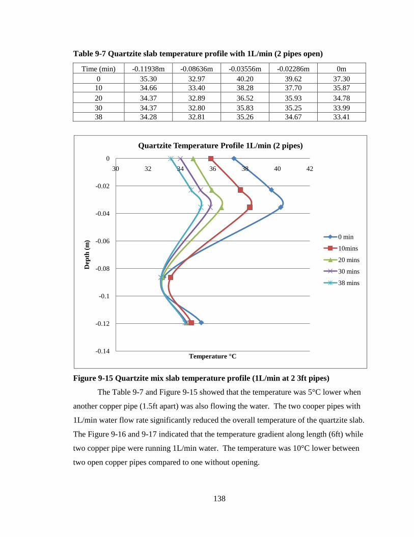
138

Table 9-7 Quartzite slab temperature profile with 1L/min (2 pipes open)

Time (min) -0.11938m -0.08636m -0.03556m -0.02286m 0m 0 35.30 32.97 40.20 39.62 37.30

10 34.66 33.40 38.28 37.70 35.87 20 34.37 32.89 36.52 35.93 34.78 30 34.37 32.80 35.83 35.25 33.99 38 34.28 32.81 35.26 34.67 33.41

Figure 9-15 Quartzite mix slab temperature profile (1L/min at 2 3ft pipes)

The Table 9-7 and Figure 9-15 showed that the temperature was 5°C lower when

another copper pipe (1.5ft apart) was also flowing the water. The two cooper pipes with

1L/min water flow rate significantly reduced the overall temperature of the quartzite slab.

The Figure 9-16 and 9-17 indicated that the temperature gradient along length (6ft) while

two copper pipe were running 1L/min water. The temperature was 10°C lower between

two open copper pipes compared to one without opening.

-0.14

-0.12

-0.1

-0.08

-0.06

-0.04

-0.02

030 32 34 36 38 40 42

Dep

th (m

)

Temperature °C

Quartzite Temperature Profile 1L/min (2 pipes)

0 min

10mins

20 mins

30 mins

38 mins

139

Figure 9-16 Quartzite slab temperature profile (1 pipe with 1L/min)

Figure 9-17 Quartzite slab temperature profile (2 pipe s with 1L/min)

30

35

40

45

50

55

0 0.5 1 1.5 2

Tem

pera

ture

°C

Distance (m)

Quartzite Slab Temperature Profile (One Pipe with 1L/min)

0m

-0.02286m

-0.03556m

-0.08636m

-0.11938m

30

32

34

36

38

40

42

44

46

0 0.5 1 1.5 2

Tem

pera

ture

°C

Distance (m)

Quartzite Slab Temperature Profile (Two Pipes with 1L/min)

0m

-0.02286m

-0.03556m

-0.08636m

-0.11938m

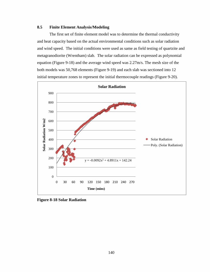
140


The first set of finite element model was to determine the thermal conductivity

and heat capacity based on the actual environmental conditions such as solar radiation

and wind speed. The initial conditions were used as same as field testing of quartzite and

metagranodiorite (Wrentham) slab. The solar radiation can be expressed as polynomial

equation (Figure 9-18) and the average wind speed was 2.27m/s. The mesh size of the

both models was 50,768 elements (Figure 9-19) and each slab was sectioned into 12

initial temperature zones to represent the initial thermocouple readings (Figure 9-20).

Figure 8-18 Solar Radiation

y = -0.0092x2 + 4.8911x + 142.24

0

100

200

300

400

500

600

700

800

900

0 30 60 90 120 150 180 210 240 270

Sola

r R

adia

tion

W/m

2

Time (mins)

Solar Radiation

Solar Radiation

Poly. (Solar Radiation)

141

Figure 9-19 Finite element mesh model

Figure 9-20 Finite element model of heating period

142

Table 9-8 Thermal conductivity and heat capacity of two slab mixes

Metagranodiorite Quartzite Thermal Conductivity (k) 1.2 1.8 Heat Capacity (Q) 800 1050

The Figure 9-21 showed the experiment data and finite element model final

temperature at one section of the quartzite slab. The thermal properties of

metagranodiorite (Wrentham) and quartzite mix were back-calculated as shown in Table

9-8.

Figure 9-21 Quartzite slab temperature profile of heat-up period

The second set of finite element model was to determine the temperature

distribution of quartzite slab and water inside the copper pipe. The temperature of

experiment data at 283 minutes was used as initial temperature for simulating water flow

conduction (Figure 9-22) and the mesh size consisted of 58,937 elements (Figure 9-23).

The Figure 9-24 and 9-25 showed temperature distribution of 1L/min water flow

-0.12

-0.1

-0.08

-0.06

-0.04

-0.02

0

30 35 40 45 50 55

Dep

th (m

)

Temperature °C

Quartzite Slab Temperature Profile Heat Up (Experiment vs FE)

283 mins

283 mins (FE)

143

rate and also showed that the temperature was fluctuated due to the uniform wall

temperature and heat flux.

Figure 9-22 Finite element model with various water flow rates

Figure 9-23 Finite element mesh model

144



22

22.5

23

23.5

24

24.5

25

25.5

26

26.5

27

0 0.2 0.4 0.6 0.8

Tem

pera

ture

°C

Distance (m)

Quartzite Slab Water Temperature 1L/mim (y-direction) (FE)

Top

Center

Bottom

-0.073025

-0.071025

-0.069025

-0.067025

-0.065025

-0.063025

-0.061025

-0.059025

-0.057025

-0.055025

22 23 24 25 26 27

Cop

per

Pipe

Dia

met

er (m

)

Temperature °C

Quartzite Slab Water Temperature Profile 1L/min (z-direction) (FE)

Entrance

Center

Exit

145

The thermal conductivity and heat capacity of quartzite slab were used for

modeling water flowing through one copper pipe at rate of 1, 2, 3, and 4L/min, and to

determine the water outlet temperature and temperature profile. The Table 9-9 to 9-13,

and, Figure 9-26 to 29 showed the temperature profile at the mid-section of the slab.

Table 9-9 Quartzite slab 1L/min (35mins)

Quartzite Slab 1L/min (35mins)

Tinitial T (°C) final ΔT (°C) (°C) LAB 23.2 30.17 6.97 FE 23.2 25.29 2.09

Figure 9-26 Quartzite slab temperature profile 1L/min (laboratory vs. finite element

analysis)

-0.12

-0.1

-0.08

-0.06

-0.04

-0.02

0

0 5 10 15 20 25 30 35 40 45 50 55

Dep

th (m

)

Temperature °C

Quartzite Slab Temperature Profile 1L/min (Experiment vs FE)

35 mins (LAB)

35 mins (FE)

146



Tinitial T (°C) final ΔT (°C) (°C) LAB 24.2 28.54 4.34 FE 24.2 26 1.80


analysis)

-0.12

-0.1

-0.08

-0.06

-0.04

-0.02

0

0 10 20 30 40 50 60

Dep

th (m

)

Temperature °C


35 mins (LAB)

35 mins (FE)

147




Figure 99-28 Quartzite slab temperature profile 3 L/min (laboratory vs. finite

element analysis)

-0.12

-0.1

-0.08

-0.06

-0.04

-0.02

0

0 10 20 30 40 50

Dep

th (m

)

Temperature °C


36 mins (LAB)

36 mins (FE)

148





analysis)

-0.14

-0.12

-0.1

-0.08

-0.06

-0.04

-0.02

0

0 10 20 30 40 50

Dep

th (m

)

Temperature C


15 mins (LAB)

15 mins (FE)

149

The temperature profile was not varied significantly at copper pipe location

(0.0381m) when the water flow rate increased for both field experiment and finite

element analysis. The water temperature of field experiment at 1 and 2L/min flow rates

were much higher than finite element analysis (Figure 9-30). This were due to different

location of water temperature measurement, for example, the field experiment measured

water temperature at one location (outlet) inside of copper pipe, and finite element

analysis integrated temperature at water outlet (exit boundary).

In addition, the quartzite slab was assumed as homogenous material to have same

thermal conductivity and heat capacity in finite element analysis. However, the quartzite

slab was consisted of aggregate and asphalt binder, which had different thermal

properties, would affect the overall heat transfer rate between the asphalt mix and water.

Figure 9-30 Quartzite slab water temperature at various water flow rate (labortory vs. finite element analysis)

0

1

2

3

4

5

6

7

8

0 0.5 1 1.5 2 2.5 3 3.5 4 4.5

Tem

pera

ture

Diff

eren

ce Δ

T, °

C

Flow Rate (L/min)

Quartzite Slab Water Temperature

LAB

FE

150

9.6 Discussion

The experiment results of all pipes open for 3ft and 6ft directions showed that the

quartzite slab yielded higher water temperauture at lower water flow rate. However,

metagranodiorite was higher at higher flow rate, this could be due to the sensitivity of

thermocouple measurement.

The experiemnt results showed that the surface temperature of quartzite slabs

could be reduced as much as 5°C for one pipe flowing water, and 10°C for two pipes

flowing water. This was the evidence that showed the effect of flowing water underneath

of higher conducitve asphalt pavement to decrease pavement temperature and reduce

Heat-Island Effect.

The water outlet temperaure of quartzite slab with one pipe open was greater than

metagranodiotite at flow rate 1L/min. The temperature differences for two slabs were

not stable for the flow rate 2L, 3L, and 4L/min. This could be due to insufficient thermal

islolation around the copper pipes and resulting in external heating during the

experiemnt.

Another reason could be the inaccurately measuring the water flow rates because

the measurement were taken by using measuing cup at the water outlet, which could be

resulting in inconsistent water flow rates.

The water temperautre distribution from finite element analysis showed that the

water temperature at the centerline was not reasch to the bounday (wall) temperature, this

was the indication of insufficient pipe length.

151

CHAPTER 10

CONCLUSION

Based on the results of this study, the following conclusions and recommendations can be

made:

1. Temperature profiles along the depth of pavements with different

structures/subsurface layers are different.

2. Predictive equations for both maximum subsurface and base temperature for

pavements with different base layers have significantly different coefficients.

3. Back-calculated thermal conductivity and heat capacity values for similar

materials but placed with different densities and gradations and with different

base layers are different.

4. Thermal conductivity values of surface+binder HMA range from 1.0 to 1.8

W/m∙K, whereas the heat capacity range from 1,100 to 1,800 J/kg∙K. For the base

materials, for the HMA materials, thermal conductivity ranges from 1.1 to 1.8

W/m∙K, whereas those for the other materials range from 1.3 to 1.5 W/m∙K. For

heat capacity, the values range from 1,200 to 1,400 J/kg∙K for the HMA materials,

and from 1,200 to 1,800 J/kg∙K for the other materials.

5. As needed one can either use ASTM E1952 or determine thermal properties of

different layers from in-place data. An alternative option is to test full depth

pavement samples under controlled conditions in the laboratory and use finite

flement analysis to back-calculate the thermal properties of the different layer.

6. Validation of temperature predicted through the use of laboratory obtained

thermal properties should be made with the help of in-place data.

7. The use of a higher conductivity aggregate, such as quartzite (1.8W/m·K), can

enhance the heat transfer efficiency to a significantly higher degree.

8. To increase heat transfer, the use of a higher conductive aggregate is most likely a

much better alternative to using commercial high conductivity additives (e.g.

copper powder) because of practical concerns.

9. The use of a reflectivity decreasing/absorptivity increasing paint on the surface of

the pavement can enhance the heat transfer efficiency.

152

10. The depth of heat exchanger is critical and an effective heat exchanger design

will be the key in extracting maximum heat from the pavement. Better contact

between the pipe and the pavement mix would lead to improved efficiency of heat

transfer.

11. The amount of heat that can be extracted depends on the surface area of the pipes

carrying the fluid.

12. Serpentine pipes can be used to improve the efficiency of heat transfer by

providing larger surface area.

13. It is possible to lower the maximum of 13.5° C of the asphalt pavements surface

temperature by flowing water underneath the pavement.

14. The reduction in temperature is affected by the type of conductivity of the mix –

higher the conductivity, higher is the reduction temperature.

15. The process of reduction in temperature can be optimized by the maximum

extraction of heat from the pavement through a fluid.

153

CHAPTER 11

FUTURE STUDY RECOMMENDATION

In the future, the study of this research should carry out both analytical and

experimental investigate on: 1.What is the effect of the outlet water temperature by using

different piping materials and working fluids? 2. How to increase the water temperature

to meet the minimum efficient requirement of turbine for it to generate electricity? 3.

How much pavement life can be extended by using asphalt pavement as solar collector?

11.1 What is the effect of the outlet water temperature by using different piping

materials and working fluids?

The material of the heat exchanger system (which consists of pipes) should have a

high conductivity and the layout should be such as to allow the exposure of the pipes to

the pavement for sufficient length to allow the fluid to reach the maximum temperature

achievable in the system. Copper material has higher thermal conductivity but it ususally

more costly, therefore, the study should selecte other alternative piping materials, for

example, graphite, iron, and PVC pipe to see the effect of replacing copper materials.

The working fluid inside the pipe should be such that it can be pumped easily and

can absorb the energy quickly (low heat capacity) such as Butane (gaseous fluid). In

applications where vaporization of the fluid is required, the fluid should ideally have a

low boiling point.

11.2 How to increase the water temperature to meet the minimum temperature

requirement of turbine to generate electricity?

The pavement temperature depends on the location of the pavement, the pavement

temperature in Worcester MA area normally is 50°C during the summer time and it will

be approximately 70°C in Houston area. The Rankin-Cycle turbine engine, for example,

requires the minimum of 70°C water temperature in order to operate at minimum

efficiency. Therefore, it is always possible to use a secondary non-energy consuming

technology, such as a solar concentrator or a water heating reservoir to increase the

temperature from the maximum temperature in the pavement to the minimum

temperature required for the end use.

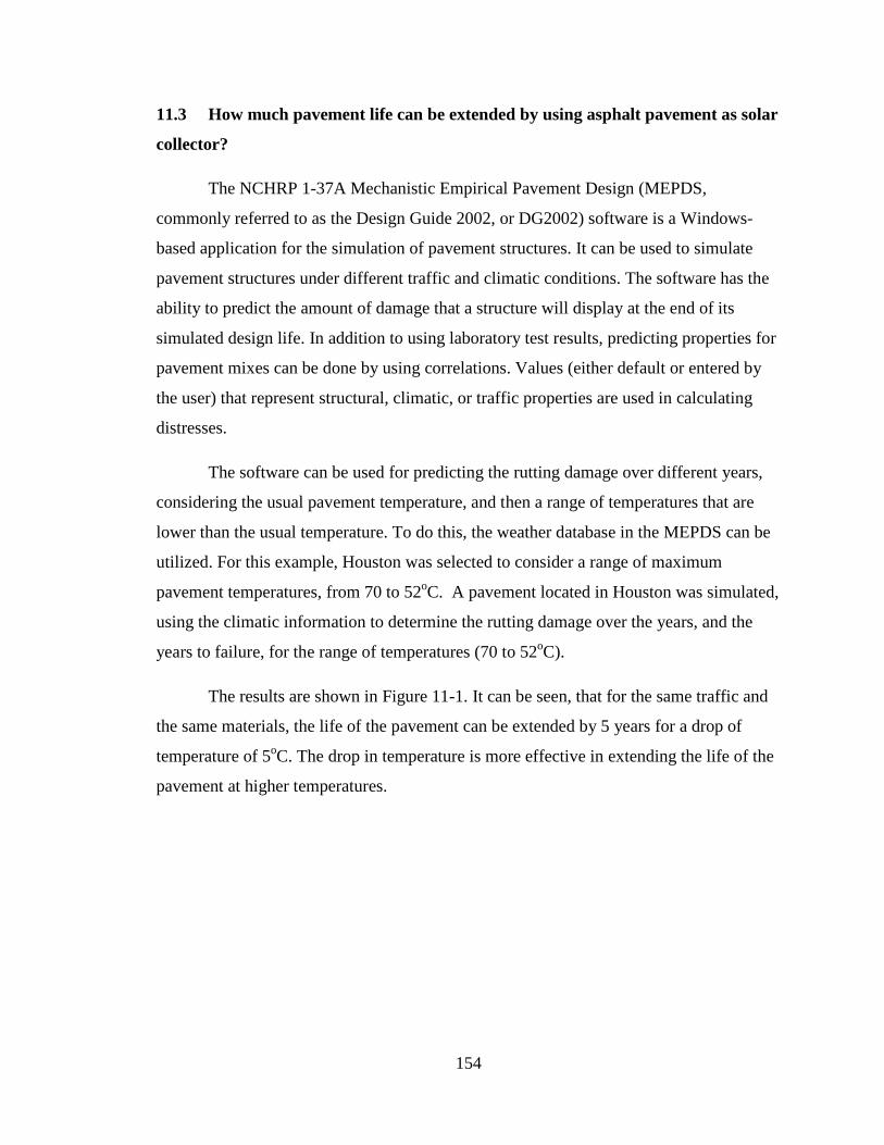
154

11.3 How much pavement life can be extended by using asphalt pavement as solar

collector?

The NCHRP 1-37A Mechanistic Empirical Pavement Design (MEPDS,

commonly referred to as the Design Guide 2002, or DG2002) software is a Windows-

based application for the simulation of pavement structures. It can be used to simulate

pavement structures under different traffic and climatic conditions. The software has the

ability to predict the amount of damage that a structure will display at the end of its

simulated design life. In addition to using laboratory test results, predicting properties for

pavement mixes can be done by using correlations. Values (either default or entered by

the user) that represent structural, climatic, or traffic properties are used in calculating

distresses.

The software can be used for predicting the rutting damage over different years,

considering the usual pavement temperature, and then a range of temperatures that are

lower than the usual temperature. To do this, the weather database in the MEPDS can be

utilized. For this example, Houston was selected to consider a range of maximum

pavement temperatures, from 70 to 52oC. A pavement located in Houston was simulated,

using the climatic information to determine the rutting damage over the years, and the

years to failure, for the range of temperatures (70 to 52o

The results are shown in Figure 11-1. It can be seen, that for the same traffic and

the same materials, the life of the pavement can be extended by 5 years for a drop of

temperature of 5

C).

oC. The drop in temperature is more effective in extending the life of the

pavement at higher temperatures.

155

Figure 11-1 Extended service life of pavement by reducing pavement temperature

0

5

10

15

20

25

50 55 60 65 70 75

Serv

ice

Life

, yea

rs

Maximum Pavement Temperature, oC

156

CHAPTER 12

REFERENCES

1. Southgate, H.F. and Deen, R.C. “Temperature Distribution within Asphalt

Pavements and its Relationship to Pavement Deflection.” Transportation Research

Record 291, Transportation Research Board, National Research Council,

Washington, DC, 1969.

2. Hermansson, Ake. “Simulation Model for Calculating Pavement Temperatures

Including Maximum Temperature.” Transportation Research Record, No. 1699,

Transportation Research Board, National Research Council, Washington, DC,

2000.

3. Park, Donh-Yeob, Buch,Neeraj, Chatti Karim. “Effective Layer Temperature

Prediction Model and Temperature Correction via Falling Weight Deflectometer

Deflections.” Transportation Research Record, No. 1764, Transportation

Research Board, National Research Council, Washington, DC, 2001.

4. Yavuzturk, C. K., Ksaibati, Chiasson, A.D., “Assessment of Temperature

Fluctuations in Asphalt Pavements Due to thermal Environment Conditions Using

a Two Dimensional, Transient Finite-Difference Approach.” Journal of Materials

in Civil Engineering, ASCE Volume 17, Issue 4, July/August 2005.

5. Solaimanian, M. and Kennedy, T.W. “Predicting Maximum Pavement Surface

Temperature Using Maximum Air Temperature and Hourly Solar Radiation.”

Transportation Research Record, No. 1417, Transportation Research Board,

National Research Council, Washington, DC, 1993.

6. Huber, G. A “Strategic Highway Research Program Report SHRP 648A: Weather

Database for the Superpave Mix Design System.” Transportation Research Board,

National Research Council, Washington, DC, 1994.

7. Solaimanian, M. and Bolzan, P. “Strategic Highway Research Program Report

SHRP –A-637: Analysis of the Integrated Model of Climate Effects on

Pavements.” Transportation Research Board, National Research Council,


157

8. Donald E. Watson, Jingna Zhang, and Powell Buzz, “Analysis of Temperature

Data for the NCAT Test Track.” Transportation Research Record, No. 1891,

Transportation Research Board, National Research Council, Washington, DC,

2004.

9. Diefenderfer, K. Brian, Al-Qadi, Imad L. and Stacey, D. “Model to Predict

Pavement Temperature Profile.” The Journal of Transportation Engineering,

ASCE, Vol. 132, No. 2, February 1, 2006.

10. Mrawira, Donath and Luca, Joseph, “Thermal Properties and Transient

Temperature Response of Full-Depth Asphalt Pavements.” Transportation

Research Record, No. 1809, Transportation Research Board, National Research

Council, Washington, DC, 2002.

11. Luca, Joseph and Mrawira, Donath “Solar-Convection Simulator for Laboratory

Investigation of Transient Temperature Fluctuations in HMAC Pavements.” 83rd

12. Luca, Joseph and Mrawira, Donath “New Measurement of thermal Properties of

Superpave Asphalt Concrete.” Journal of Materials in Civil Engineering ASCE

Volume 17, Issue 1, (January/February 2005).

Annual Meeting of the Transportation Research Board, Washington, DC, 2004.

13. Bijsterveld, W. T. van, Houben, Scarpas, A. and Molenaar, A. A. A. „Effect of

Using Pavement as Solar Collector on Pavement Temperature and Structural

Response." Journal of The Transportation Research Record, No No. 1778,

Transportation Research Board, National Research Council, Washington, DC

2001

14. Hasebel M., Kamikawa Y. and Meiarashi S. “Thermoelectric Generators using

Solar Thermal Energy in Heated Road Pavement.” 2006 International Conference

on Thermoelectrics, IEEE.

15. The United States Environmental Protection Agency, “Heat Island Effect”,

http://www.epa.gov/hiri/

16. Martina Soderlund, Stephen T. Muench, Kim A. Willoughby, Jeffrey S.

Uhlmeyer, Jim Weston, “Green Roads: A Sustainability Rating System for

Roadways” Transportation Research Board 87th Annual Meeting, 2008

http://trb.metapress.com/content/?Author=A.+Scarpas�

http://trb.metapress.com/content/?Author=A.+A.+A.+Molenaar�

158

17. Mark Belshe, Kamil E. Kaloush, Jay S. Golden, Michael S. Mamlouk, Patrick

Phelan, “Asphalt-Rubber Asphalt Concrete Friction Course Overlays as Pavement

Preservation Strategy for Portland Cement Concrete Pavement” Transportation

Research Board 86th Annual Meeting, 2007

18. Gui, Jooseng Gavin, Phelan, Patrick E., Kaloush, Kamil E. and Golden, Jay S.

“Impact of Pavement Thermophysical Properties on Surface Temperatures.”

Journal of Materials in Civil Engineering, Vol. 19, No. 8, August 1, 2007

19. Kanok Boriboonsomsin, Farhad Reza, “Mix Design and Benefit Evaluation of

High Solar Reflectance Concrete for Pavements” Transportation Research

Record: Journal of the Transportation Research Board No. 2011. 2007.

20. Frank W. Schmidt, Robert E. Henderson, Carl H. Wolgemuth “Introduction to

Thermal Sciences: Thermodynamics, Fluid Dynamics, Heat Transfer.” John

Wiley & Sons, 1993.

21. J. E. Vehrencamp, “Experimental Investigation of Heat Transfer at an Air-Earth

Interface.” Transportation, American Geophysical Union, Vol. 34, No. 1, 1953.

22. Bruce R.Munson, Donald F.Young, and Theodore H.Okishi, “Foundamentals of

Fluid Mechanics.” 5th edition, John Wiley & Sons (Asia) Pte Ltd. 2005.

23. Daryl L. Logan, „A First Course in the Finite Element Method“, 2nd Edition,

PWS Publish Company, 1993

24. Nazarian,Soheil and Alvarado Gisel, “Impact of Temperature Gradient on

Modulus of Asphaltic Concrete Layers, Journal of Materials in Civil

Engineering.” Vol. 18, No. 4, July/August 2006.

25. National Cooperative Highway Research Program (NCHRP). “Guide for

Mechanistic-Empirical Design.” Transportation Research Board, Washington,

DC, Design Inputs, March 2004.

26. COMSOL. “Heat Transfer Module User’s Guide.” COMSOL Multiphysics 3.2,

2005

27. Côté Jean and Konrad Jean-Marie, “Estimating Thermal Conductivity of

Pavement Granular Materials and Subgrade Soils.” Transportation Research

159

Record, 1967, Transportation Research Board, National Research Council,


28. Christoph Clauser, Ernst Huenges, “Thermal Conductivity of Rocks and

Minerals.” American Geophysical Union, 1995.

160

APPENDIX A

SIX EXISTING PAVEMENT THERMOCOUPLE LOCATIONS

Figure A-1 G Sample - Highway-HMA layers over HMA base with different NMAS

Figure A-2 S Sample -HMA layers over PMRAP base

T1- 1” above surface (air)

T2- Surface

T3- 1” (25.4mm) below surface

T4- 1 5/8” (41.275mm)

T5-3 1/8” (79.375mm)

T6- 4 1/4” (107.95mm)

ρ=2377kg/m3

ρ=2377kg/m3

ρ=2084kg/m3

145m

m

150mm

S-sample


T2- Surface


T4- 2 1/4” (57.15mm)

T5- 4” (101.6mm)

T6- 6” (152.4mm)

ρ=2377kg/m3

ρ=2377kg/m3

ρ=2084kg/m3

200m

m

150mm

G-Sample

161

Figure A-3 M Sample- HMA layers over Foamed Asphalt base

Figure A-4 R Sample- HMA layers over cement treated base


T2- Surface


T4- 2” (50.8mm)

T5-4 1/4” (107.955mm)

T6- 6 3/4” (171.45mm)

ρ=2386kg/m3

ρ=2209kg/m3

ρ=2033kg/m3

277m

m

150mm

R-sample


T2- Surface


T4- 1 3/4” (44.45mm)

T5-3 3/4” (95.25mm)

T6- 5 1/2” (139.7mm)

ρ=2284kg/m3

ρ=2284kg/m3

ρ=2021kg/m3

210m

m

150mm

M-sample

162

Figure A-5 P401 Sample- HMA layers of same NMAS

Figure A-6 FR Sample- HMA layers of different types two lifts


T2- Surface


T4- 2” (50.8mm)

T5- 2 3/4” (69.85mm)

T6- 4 1/2” (107.95mm)

ρ=2549kg/m3

ρ=2557kg/m3

ρ=2467.73kg/m3

152m

m

150mm

FR over PM


T2- Surface


T4- 3.75” (95.25mm)

T5- 6.5” (165.1mm)

T6- 9” (228.6mm)

ρ=2472.7kg/m3

ρ=2517.9kg/m3

ρ=2467.73kg/m3

298m

m

150mm

P401

163

APPENDIX B

DETERMINE THERMAL PROPERTIES OF R, P401, M, AND FR SAMPLES

Figure B-1 R sample temperature at T2 (finite element predicted vs. laboratory results)


0

10

20

30

40

50

60

0 60 120 180 240 300 360 420 480 540 600 660 720

Tem

pera

true

°C

Time (mins)

R Sample T2 (k=1.8W/m·K, C=1800J/kg)

LAB

FE

0

10

20

30

40

50

60

0 60 120 180 240 300 360 420 480 540 600 660 720

Tem

pera

true

°C

Time (mins)


LAB

FE

164



0

10

20

30

40

50

60

0 60 120 180 240 300 360 420 480 540 600 660 720

Tem

pera

true

°C

Time (mins)


LAB

FE

0

10

20

30

40

50

0 60 120 180 240 300 360 420 480 540 600 660 720

Tem

pera

true

°C

Time (misn)


LAB

FE

165


Figure B-6 P401 sample temperature at T2 (finite element predicted vs. laboratory results)

0

10

20

30

40

50

0 60 120 180 240 300 360 420 480 540 600 660 720

Tem

pera

true

°C

Time (mins)


LAB

FE

0

10

20

30

40

50

60

70

0 60 120 180 240 300 360 420 480 540 600 660 720

Tem

epra

ture

°C

Time (mins)

P401 T2 (k=1.6W/m·K, C=1200J/kg)

LAB

FE

166



0

10

20

30

40

50

60

0 60 120 180 240 300 360 420 480 540 600 660 720

Tem

epra

ture

°C

Time (mins)

P401 T3 (k=1.6W/m·K, C=1200J/kg)

LAB

FE

0

10

20

30

40

50

0 60 120 180 240 300 360 420 480 540 600 660 720

Tem

epra

ture

°C

Time (mins)

P401 T4 (k=1.6W/m·K, C=1200J/kg)

LAB

FE

167


Figure B-10 P401 sample temperature at T6 (finite element predicted vs. laboratory

results)

0

10

20

30

40

50

0 60 120 180 240 300 360 420 480 540 600 660 720

Tem

epra

ture

°C

Time (mins)

P401 T5 (k=1.6W/m·K, C=1200J/kg)

LAB

FE

0

10

20

30

40

0 60 120 180 240 300 360 420 480 540 600 660 720

Tem

epra

ture

°C

Time (mins)

P401 T6 (k=1.6W/m·K, C=1200J/kg)

LAB

FE

168

Figure B-11 M sample temperature at T2 (finite element predicted vs. laboratory results)


0

10

20

30

40

50

60

0 60 120 180 240 300 360

Tem

pera

ture

°C

Time (mins)

M Sample T2 (k=1.5W/m·K, C=1800J/kg)

LAB

FE

0

10

20

30

40

50

0 60 120 180 240 300 360

Tem

pera

ture

°C

Time (mins)


LAB

FE

169



0

10

20

30

40

50

0 60 120 180 240 300 360

Tem

pera

ture

°C

Time (mins)


LAB

FE

0

10

20

30

40

0 60 120 180 240 300 360

Tem

pera

ture

°C

Time (mins)


LAB

FE

170


Figure B-16 FR sample temperature at T2 (finite element predicted vs. laboratory results)

0

10

20

30

40

0 60 120 180 240 300 360

Tem

pera

ture

°C

Time (mins)


LAB

FE

0

10

20

30

40

50

60

0 60 120 180 240 300 360

Tem

pera

ture

°C

Time (mins)

FR Sample T2 (k=1.5W/m·K, C=1200J/kg)

LAB

FE

171



0

10

20

30

40

50

60

0 60 120 180 240 300 360

Tem

pera

ture

°C

Time (mins)


LAB

FE

0

10

20

30

40

50

0 60 120 180 240 300 360

Tem

pera

ture

°C

Time (mins)


LAB

FE

172



0

10

20

30

40

50

0 60 120 180 240 300 360

Tem

pera

ture

°C

Time (mins)


LAB

FE

0

10

20

30

40

50

0 60 120 180 240 300 360

Tem

pera

ture

°C

Time (mins)


LAB

FE

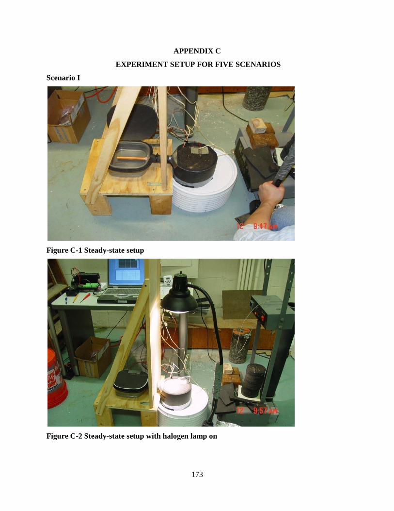
173

APPENDIX C

EXPERIMENT SETUP FOR FIVE SCENARIOS

Scenario I

Figure C-1 Steady-state setup

Figure C-2 Steady-state setup with halogen lamp on

174

Scenario II

Figure C-3 Complied 5 asphalt pavement testing

Figure C-4 Complied 5 asphalt pavements testing without halogenn lamp on

175

Scenario III and VI

Figure C-5 Transient testing setup

Scenario V

Figure C-6 Glass chips-Apshalt mix placed on top of asphalt sample

176

Figure C-7 Tinted glass placed on top of asphalt sample

177

APPENDIX D

DETERMINE THERMAL PROPERTIES OF QUARTZITE, LIMESTONE, AND

METAGRANODIORITE (SMALL SCALE)

Figure D-1 Quartzite sample temperature at T2 (finite element predicted vs. laboratory

results)


results)

0102030405060708090

0 60 120 180 240 300 360

Tem

pera

ture

°C

Time (mins)

Quartzite Mix Temperauture at T2 (k=1.8W/m·K, C=1050J/kg)

LABFE

0102030405060708090

0 60 120 180 240 300 360

Tem

pera

ture

°C

Time (second)

Quartzite Mix Temperature at T3 (k=1.8W/m·K, C=1050J/kg)

LABFE

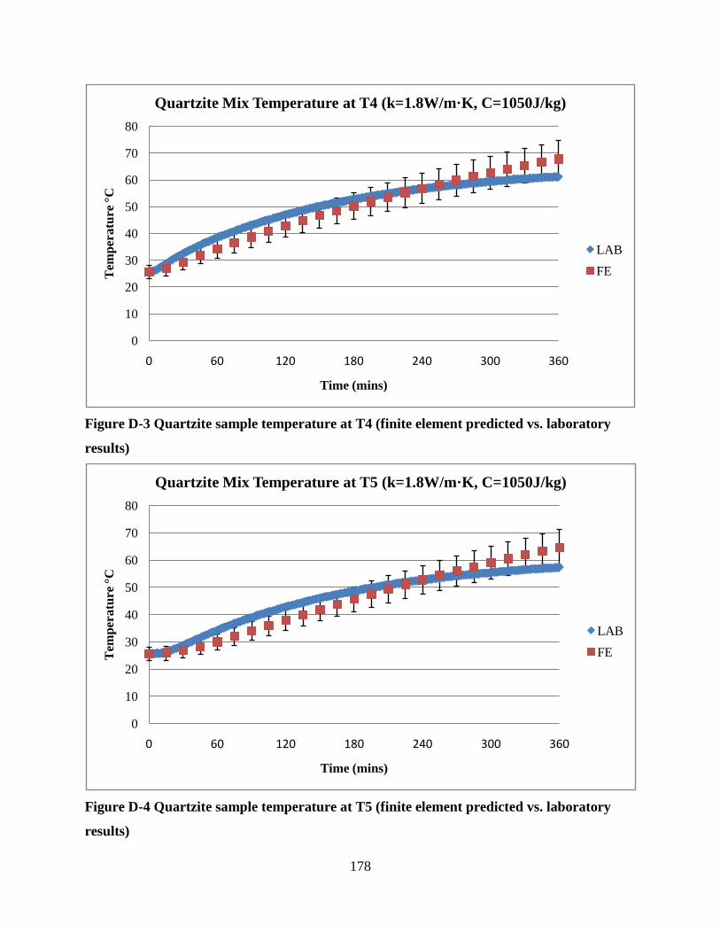
178


results)


results)

0

10

20

30

40

50

60

70

80

0 60 120 180 240 300 360

Tem

pera

ture

°C

Time (mins)


LABFE

0

10

20

30

40

50

60

70

80

0 60 120 180 240 300 360

Tem

pera

ture

°C

Time (mins)


LABFE

179

Figure D-5 Limestone sample temperature at T3 (finite element predicted vs. laboratory

results)


results)

0

10

20

30

40

50

60

70

0 30 60 90 120 150 180

Tem

pera

ture

°C

Time (mins)

Limestone Mix Temperature at T3 (k=1.4W/m·K, Q=950 J/kg)

LAB

FE

0

10

20

30

40

50

60

0 30 60 90 120 150 180

Tem

pera

ture

°C

Time (mins)


LAB

FE

180


results)

Figure D-8 Metagranodiorite sample temperature at T2 (finite element predicted vs.

laboratory results)

0

10

20

30

40

50

60

0 30 60 90 120 150 180

Tem

pera

ture

°C

Time (mins)


LAB

FE

0

10

20

30

40

50

60

70

80

90

100

0 60 120 180 240 300 360

Tem

pera

ture

°C

Time (second)

Metagranodiorite Mix Temperature at T2 (k=1.2W/m·K, C=800J/kg)

LAB

FE

181


laboratory results)


laboratory results)

0

10

20

30

40

50

60

70

80

90

0 60 120 180 240 300 360

Tem

pera

ture

°C

Time (second)

Metagranodiorite Mix Temperature at T3 (k=1.2W/m·K, C=800J/kg)

LAB

FE

0

10

20

30

40

50

60

70

80

90

0 60 120 180 240 300 360

Tem

pera

ture

°C

Time (second)

Metagranodiorite Temperature at T4 (k=1.2W/m·K, C=800J/Kg)

LAB

FE

182


laboratory results)

0

10

20

30

40

50

60

70

80

0 60 120 180 240 300 360

Tem

pera

ture

°C

Time (second)

Metagranodiorite Mix Temperature at T5 (k=1.2W/m·K, C=800J/Kg)

LAB

FE

183

APPENDIX E

SKETCH AND DIMENSION OF HAND-COMPACTED SAMPELS

Figure F-1 100% Metagranodiorite mix

Figure F-2 100% Quartzite mix

100% Quartzite

T7- 89.3mm

T10- Water outflow

T1-25.4mm above

surface

T2- surface

T3, T4, T5- 25.4 mm below

surface

150mm

102

mm

¼”Copper Tube

T9- Inflow

T6- 50.8mm

T8- Air Temp

100% Metagranodiorite

T7- 89.3mm

T10- Water outflow


T2- surface


surface

150mm

102

mm

¼”Copper Tube

T9- Inflow

T6- 50.8mm

T8- Air Temp

184

Figure F-3 50% Quartzite on the top and 50% Metagranodiorite on the bottom

Figure F-4 35% Metagranodiorite on the top, 30% quartzite in the center layer, and 35%

Metagranodiorite on the bottom

30% Quartzite

T7- 89.3mm

T10- Water outflow


T2- surface


surface

150mm

102

mm

¼”Copper Tube

T9- Inflow

T6- 50.8mm

T8- Air Temp

Metagranodiorite

50% Quartzite

T7- 89.3mm

T10- Water outflow


T2- surface

T3, T4, T5- 25.4 mm

below surface

150mm

102

mm

¼”Copper Tube

T9- Inflow

T6- 50.8mm

T8- Air Temp


185

Figure F-5 100% Metagranodiorite mix with Portland cement placed around copper pipe

Figure F-6 100% Quartzite mix with a copper pipe consists 6 rings

Pipe with rings

T7- 89.3mm

T10- Water outflow


T2- surface


surface

150mm

102

mm

¼”Copper Tube

T9- Inflow

T6- 50.8mm

T8- Air Temp

100% Quartzite

0.5” thick Copper rings

Space with 0.8”

Portland cement

T7- 89.3mm

T10- Water outflow


T2- surface


surface

150mm

102

mm

¼”Copper Tube

T9- Inflow

T6- 50.8mm

T8- Air Temp


186

Figure F-7 100% Quartzite mix with a rough surface copper pipe


Rough Pipe

T7- 89.3mm

T10- Water outflow

T2- surface


surface

150mm

102

mm

¼”Copper Tube

T9- Inflow

T6- 50.8mm

T8- Air Temp

100% Quartzite

187

APPENDIX F

DETERMINE THERMAL PORPERTIES OF METAGRANODIORITE AND

QUARTZITE (HAND-COMPACTED SAMPLES)

Figure E-1 Metagranodiorite sample temperature at T2 (finite element predicted vs.

laboratory results)


laboratory results)

0

10

20

30

40

50

60

70

80

0 60 120 180 240 300 360

Tem

pera

ture

°C

Time (mins)

100% Metagranodiorite Mix Temperature at T4 (k= 1.1W/m·K, C= 900 J/kg)

LABFE

01020304050607080

0 60 120 180 240 300 360

Tem

pera

ture

°C

Time (mins)

100% Metagranodiorite Mix Temperature at T6 (k= 1.1 W/m·K, C= 900 J/kg)

LABFE

188


laboratory results)

Figure E-4 Quartzite sample temperature at T4 (finite element predicted vs. laboratory

results)

0

10

20

30

40

50

60

70

80

0 60 120 180 240 300 360

Tem

pera

ture

°C

Time (mins)

100% Metagrandiorite Mix Temperature at T7 (k=1.1W/m·K, C= 900 J/kg)

LABFE

0

10

20

30

40

50

60

70

80

0 60 120 180 240 300 360

tem

pera

ture

°C

Time (mins)

100% Quartzite Mix Temperature at T4 (k=2.0 W/m ·K, C=950 J/kg)

LAB

FE

189


results)


results)

0

10

20

30

40

50

60

70

80

0 60 120 180 240 300 360

tem

pera

ture

°C

Time (mins)

100% Quartzite Mix Temperature at T6 (k=2.0 W/m·K, C=950 J/kg)

LAB

FE

0

10

20

30

40

50

60

70

80

0 60 120 180 240 300 360

Tem

pera

ture

°C

Time (mins)

100% Quartzite Mix Temperature at T7 (k=2.0 W/m·K, C=950 J/kg)

LAB

FE

190

APPENDIX G

LARGE SCALE PAVEMENT (SLAB) PERPARATION

Figure G-1 Cart with thermocouple at the bottom

Figure G-2 Lay down of mix

191

Figure G-3 Compaction

Figure G-4 Fixing thermocouples

192

Figure G-5 Copper pipe frame

Figure G-6 Close-up of slab showing copper tube and thermocouples at different depths

193

Figure G-7 Completed slab ready for testing

capture solar energy and reduce heat-island effect from

Documents