Capturing Label Distribution: A Case Study in NLI

Shujian Zhang Chengyue Gong Eunsol ChoiDepartment of Computer Science, The University of Texas at Austin

AbstractWe study estimating inherent human disagree-ment (annotation label distribution) in naturallanguage inference task. Post-hoc smoothingof the predicted label distribution to matchthe expected label entropy is very effective.Such simple manipulation can reduce KL di-vergence by almost half, yet will not improvemajority label prediction accuracy or learn la-bel distributions. To this end, we introduce asmall amount of examples with multiple refer-ences into training. We depart from the stan-dard practice of collecting a single referenceper each training example, and find that col-lecting multiple references can achieve betteraccuracy under the fixed annotation budget.Lastly, we provide rich analyses comparingthese two methods for improving label distri-bution estimation.

1 Introduction

Recent papers (Pavlick and Kwiatkowski, 2019;Nie et al., 2020) have shown that human annota-tors disagree on solving natural language inference(NLI) tasks (Dagan et al., 2005; Bowman et al.,2015), which decides whether hypothesis h is truegiven premise p. Such disagreement is not an an-notation artifact but rather exhibits the judgementof annotators with differing interpretations of en-tailment (Reidsma and op den Akker, 2008). Westudy how to estimate such distribution of labelsfor NLI task, as introduced in newly proposed eval-uation dataset (Nie et al., 2020) which contains 100human labels per example.

Without changing model architectures (Devlinet al., 2019), we focus on improving predicted labeldistribution. We introduce two simple ideas: cali-bration and training with examples with multiplereferences (multi-annotated). Estimating label dis-tribution is closely related to calibration (Rafteryet al., 2005), which studies how aligned is the pre-dicted probability distribution with empirical likeli-hood, in this case, human label distribution. When

trained naively with cross entropy loss on unam-biguously annotated data (examples with a singlelabel), models generate a over-confident distribu-tion (Thulasidasan et al., 2019) putting a strongweight on a single label. Observing that the entropyof predicted distribution is substantially lower thanthat of human label distribution, we calibrate thisdistribution such that two distributions have com-parable entropy via temperature scaling (Guo et al.,2018) and label smoothing (Szegedy et al., 2016).

While such calibration shows strong gains, re-ducing the KL divergence (Kullback and Leibler,1951) between predicted and human distribution byroughly half, it does not improve accuracy. Priorworks introduce inherent human disagreement intoevaluation, and we further embrace such ambigu-ity into training. Almost all nlp datasets (Wanget al., 2019; Rajpurkar et al., 2016) present singlereference for training examples while collectingmultiple references for examples in the evaluationdataset. We show that, under the same annotationbudget, adding a small amount of multi-annotatedtraining, at the cost of decreasing total examplesannotated, improves label distribution estimationas well as prediction accuracy. Lastly, we providerich analyses on differences between calibrationapproach and multi-annotation training approach.To summarize, our contributions are the following:

• Introduce calibration techniques to improvelabel distribution estimation in natural lan-guage inference task.

• Present an empirical study showing collect-ing multiple references for a small numberof training examples is more effective thanlabeling as many examples as possible, underthe same annotation budget.

• Study the pitfalls of using distributional met-rics to evaluate human label distribution.

arX

iv:2

102.

0685

9v1

[cs

.CL

] 1

3 Fe

b 20

21

ChaosSNLI (H = 0.563) ChaosMNLI (H = 0.732)JSD↓ KL ↓ acc (old/new)↑ H JSD ↓ KL ↓ acc (old/new) ↑ H

Best reported (all)) 0.220 0.468 0.749 / 0.787 0.305 0.665 0.674 / 0.635Est. human 0.061 0.041 0.775 / 0.940 0.069 0.038 0.660 / 0.860RoBERTa (all) 0.229 0.505 0.727 / 0.754 0.307 0.781 0.639 / 0.592

RoBERTa (our reimpl.,all) 0.230 0.502 0.723 / 0.754 0.310 0.790 0.642 / 0.594RoBERTa (our reimpl.,subset) 0.242 0.548 0.684 / 0.710 0.345 0.308 0.799 0.670 / 0.604 0.414+ calib (temp. scaling) 0.202 0.281 0.684 / 0.710 0.569 0.233 0.324 0.670 / 0.604 0.720+ calib (pred smoothing) 0.222 0.326 0.684 / 0.710 0.566 0.245 0.347 0.670 / 0.604 0.722+ calib (train smoothing) 0.221 0.338 0.688 / 0.710 0.537 0.252 0.372 0.680 / 0.602 0.701+ multi-annot 0.183 0.203 0.690 / 0.740 0.649 0.190 0.179 0.646 / 0.690 0.889+ pred smoothing & multi-annot 0.202 0.196 0.690 / 0.740 0.773 0.209 0.189 0.646 / 0.690 0.977

Table 1: Main results: H next to the dataset name on the top row refers to the entropy value of human label dis-tribution. All calibration methods show significant gains on distribution metrics, but introducing multi-annotatedexamples into training shows the strongest results. The top block results are from Nie et al. (2020), and rows ingrey color are not strictly comparable (evaluated on the different set).

2 Evaluation

2.1 Data

We use the training data from the origi-nal SNLI (Bowman et al., 2015) and MNLIdataset (Williams et al., 2018), each contain-ing 592K and 392K instances. We evaluate onChaosNLI dataset (Nie et al., 2020), which iscollected the same way as original SNLI dataset,but contains 100 labels per example instead offive.1 We repartition this data to simulate a multi-annotation setting, whether having more than onelabel per training example can be helpful. Wereserve 500 randomly sampled examples for evalu-ation and use the rest for training.2

2.2 Metrics

Following Nie et al. (2020), we report classifi-cation accuracy, Jensen-Shannon Divergence (En-dres and Schindelin, 2003), Kullback-Leibler Di-vergence (Kullback and Leibler, 1951), comparinghuman label distributions with the softmax out-puts of models. The accuracy is computed twice,once against aggregated gold labels in the origi-nal dataset (old), and against the aggregated labelfrom 100-way annotated dataset (new). In addition,we report the model prediction label distributionentropy H .

1It covers SNLI, MNLI, and αNLI (Bhagavatula et al.,2020), and we focus our study on the first two datasets as theyshow more disagreement among the annotators.

2The original datasets split data such that premise does notoccur in both train and evaluation set. This random repartitionbreaks that assumption, now a premise can occur in both train-ing and evaluation with different hypotheses. However, wefind that the performance on examples with/without overlap-ping premise in the training set does not vary significantly.

2.3 Comparison Systems

We use RoBERTa (Liu et al., 2019) based classifica-tion model, i.e., encoding concatenated hypothesisand premise and pass the resulting [CLS] represen-tation through a fully connected layer to predict thelabel distribution, trained with cross entropy loss.

Calibration Methods We experiment with threecalibration methods (Guo et al., 2018; Miller et al.,1996). The first two methods are post-hoc and donot require re-training of the model. For all meth-ods, we tuned a single scalar hyperparameter perdataset such that prediction label distribution en-tropy that matches that of human label distribution.

• temp. scaling: scaling by multiplying non-normalized logits by a scalar hyperparameter

• pred smoothing: process softmaxed label dis-tribution by moving α probability mass fromthe label with the highest mass to the all labelsequally

• train smoothing: process training label dis-tribution by shifting α probability mass fromthe gold label to the all labels equally

Multi-Annotated Data Training We comparethe results under the fixed annotation budget, i.e.,the number of annotations collected. We vary num-ber of examples annotated and the number of anno-tations per example. We remove 10k randomly-sampled single annotated examples from train-ing portion, and add 1k 10-way annotated exam-ples from the re-partitioned training portion of theChaosNLI dataset. For each example, we sample10 out of 100 annotations. We first train model withsingle-annotated examples and further finetune it

#annot ChaosSNLI (H = 0.563) ChaosMNLI (H = 0.732)JSD↓ KL↓ acc (old/new)↑ H JSD↓ KL↓ acc (old/new) ↑ H

RoBERTa 0.250 0.547 0.676 / 0.688 0.363 0.312 0.753 0.628 / 0.578 0.444+ pred smoothing 150K 0.231 0.342 0.676 / 0.688 0.573 0.253 0.363 0.628 / 0.578 0.737+ multi-annot 0.186 0.219 0.684 / 0.732 0.643 0.195 0.183 0.616 / 0.684 0.910

RoBERTa 0.264 0.534 0.668 / 0.656 0.445 0.319 0.686 0.552 / 0.496 0.518+ pred smoothing 15K 0.256 0.412 0.668 / 0.656 0.594 0.276 0.424 0.552 / 0.496 0.752+ multi-annot 0.293 0.336 0.624 / 0.674 0.985 0.252 0.269 0.546 / 0.554 1.026

Table 2: Performances with smaller annotation budget. With smaller annotation budget, using multi-annotationcan hurt accuracy on noisier evaluation setting (old), but still shows improvements on less noisy setting (new) andon most distribution metrics.

with multi-annotated examples.3

2.4 Results

Table 1 compares the published results from Nieet al. (2020) to our reimplementation and proposedapproaches. As we set aside some 100-way anno-tated examples for training, our results are on therandomly selected subset of evaluation dataset, forsanity check, we report our re-implemented resultson the full set, which matches the reported results.

The initial model was over confident, withsmaller predicted label entropy (0.345/0.414) com-pared to the annotated label distribution entropy(0.563/0.732). We find all calibration methodsimprove performance on both distribution metrics(JSD and KL). Temperature scaling yields slightlybetter results than label smoothing, consistent withthe findings from Desai and Durrett (2020) whichshows temperature scaling is better for in-domaincalibration compared to label smoothing.

Finetuning on multi-annotated data improves dis-tribution metrics and the accuracy, yet the perfor-mance is below the estimated human performance.This approach seems to be effective at capturingthe inherent ambiguity, and to learn label noisefrom the crowdsourced dataset. Our method showsmore gains in accuracy on newly 100-way anno-tated dataset, with less noisy majority label, thanthe majority label from the original 5-way devel-opment set. We rerun the baseline and this modelthree times with different random seeds to deter-mine the variance, which is small.4 Using bothmulti-annotated data and calibration show mixedresults, suggesting that calibration is not neededwhen you have multi-annotated examples.

Table 2 studies scenarios with smaller annotation3We find merging multi-annotation data with single-

annotation data does not show improvements.4The standard deviation value of KL on all method / dataset

pairs is lower than 0.01.

budgets. Similar trend holds, yet in the smallestannotation budget setting, the gains in distributionmetrics from fine-tuning approach comes at thecost of accuracy drop, potentially as the model isnot exposed to diverse examples.

(a) Human label entropy (b) RoBERTa prediction entropy

0.0 0.5 1.0

45

90

0.0 0.5 1.0

45

90

(c) Calibrated RoBERTa (d) Multi-annot RoBERTa

0.0 0.5 1.0

45

90

0.0 0.5 1.0

45

90

Figure 1: The empirical distribution of label/predictionentropy on ChaosSNLI dataset, where x-axis denotesthe entropy value and y-axis denotes the example counton the entropy bin. Initial model prediction showslow entropy values for many examples, being over-confident. Post-hoc calibration successfully shifts thedistribution to be less confident, but with artifacts ofnot being confident on any examples. Finetuning onthe small amount of multi-annotated data (d) success-fully simulate the entropy distribution of human labels.

3 Analysis

Can we estimate the distribution of ambiguousand less ambiguous examples? Figure 1 showsthe empirical example distribution over the entropybins: The leftmost plot shows the annotated humanlabel entropy over our evaluation set, and the plotnext to it shows the prediction entropy of the base-line RoBERTa model predictions. Trained only onsingle label training examples, the model is over-confident about its prediction. With label smooth-ing, the over-confidence problem is relieved, but

0.2

0.4

0.2

0.4

0.2

0.40.00 - 0.460.46 - 0.640.64 - 0.720.72 - 0.820.82 - 1.09

α=0 α=0.3 α=0.6

Figure 2: Jensen-Shannon Divergence (JSD) on dif-ferent label distribution entropy bins on ChaoSNLIdataset. Before label smoothing, the scores are lowerfor ambiguous examples, but the results swap after fur-ther smoothing.

still does not match the distribution of ground truth(see plot (c)). Training with multi-annotated data(plot (d)) makes the prediction distribution similarto the ground truth.

Are label distribution metrics reliable? Nieet al. (2020) suggests that ambiguous examples forhumans are also more challenging for models inthis dataset. We aware that this observation holdsfor accuracy measure but not for distribution met-rics. Figure 2 demonstrates that when we furthersmooth the label distribution, JSD is better on sup-posedly more challenging examples where humansdisagree. We find smoothing, which improves dis-tribution metrics but not accuracy, can generateunlikely label distributions, e.g. assigning high val-ues to both entailment and contradiction label. Wehypothesize that humans often confuse betweenneutral and one of the two labels, not betweenthese two labels. To quantify this intuition, wecompute the average minimal probability assignedto either contradiction or entailment label: minvalue for human annotation is only 0.03, and 0.02for the baseline model. We notice label smoothingincreases min value to 0.06 and finetuning withmulti-annotated increases the min value to 0.04.

We summarize studies not covered in our eval-uation section (details in the appendix). Do theresults hold for other model architecture or big-ger model? Yes. Our results show the same pat-tern with ALBERT model (Lan et al., 2020) and thelarger variant of RoBERTa model. Is the methodsensitive to the number of labels per trainingexample? No. We try different label strategies(5-way, 10-way, or 20-way), while keeping the to-tal number of annotation fixed, and observe nochanges. What happens if you keep smooth-ing the distribution? We choose label smoothinghyper-parameter such that the predicted label distri-bution entropy matches that of human annotation

distribution. However, we notice keep smoothingmodel prediction further (α = 0.125 → 0.4 forSNLI) brings further gains. Should we carefullyselect which examples to have multiple annota-tions? Maybe. We experiment on how to selectexamples to have multiple annotations, using theideas from Swayamdipta et al. (2020). We finetunewith 100 most hard-to-learn, most easy-to-learn,most ambiguous, and randomly sample examplesfrom 1K examples. Easy-to-learn examples, withlowest label distribution entropy, are the least effec-tive, but the difference is small in our settings.

4 Related Work

Human Disagreement in NLP Prior workshave covered inherent ambiguity in different lan-guage interpretation tasks. Aroyo and Welty (2015)demonstrates that it is improper to believe that thereis a single truth for crowdsourcing. Question an-swering, summarization and translation literatureshave been collecting multiple references per ex-ample for evaluation. Most related to our work,Pavlick and Kwiatkowski (2019) carefully exam-ines the distribution behind human references andNie et al. (2020) has conducted a larger-scale datacollection. To capture the subtleties of NLI task,Glickman et al. (2005); Zhang et al. (2017); Chenet al. (2020) introduce graded human responseson the subjective likelihood of an inference. Inthis work, we explicitly focus on improving labeldistribution estimation on the existing benchmarks.

Efficient Labeling Previous works have ex-plored different data labeling strategies for NLPtasks, from active learning (Fang et al., 2017), pro-viding fine-grained rationales (Dua et al., 2020) tomodel prediction validation approaches (Kratzwaldet al., 2020). Recent work (Mishra and Sachdeva,2020) studies how much annotation is necessaryto solve NLI task. In this work, we study collect-ing multiple references per each training example,which has not been explored to our understanding.

Calibration in NLP (Nguyen and O’Connor,2015; Ott et al., 2018) could make predictionsmore useful and interpretable. Large-scale pre-trained models are not well calibrated (Jianget al., 2018), and its predictions tend to be over-confident (Malkin and Bilmes, 2009; Thulasidasanet al., 2019). Calibration has been studied for pre-trained language models for classification (Desaiand Durrett, 2020), reading comprehension (Ka-

math et al., 2020) and in general machine learningtopics (e.g. Guo et al., 2018; Pleiss et al., 2017).While these works focus on improving robustnessto out-of-domain distribution, we study predictinglabel distributions.

5 Conclusion

We study capturing inherent human disagreementin the NLI task through calibration and using asmall amount of multi-annotated training examples.Annotating fewer examples many times as apposedto annotating as many examples as possible canbe useful for other language understanding taskswith ambiguity and generation tasks where multiplereferences are valid and desirable (Hashimoto et al.,2019).

Acknowledgements

The authors thank Greg Durrett, Raymond Mooney,and Michael Zhang for helpful comments on thepaper draft.

ReferencesLora Aroyo and Chris Welty. 2015. Truth is a lie:

Crowd truth and the seven myths of human annota-tion. AI Mag., 36:15–24.

Chandra Bhagavatula, Ronan Le Bras, ChaitanyaMalaviya, Keisuke Sakaguchi, Ari Holtzman, Han-nah Rashkin, Doug Downey, Wen-tau Yih, and YejinChoi. 2020. Abductive commonsense reasoning. InICLR.

Samuel R. Bowman, Gabor Angeli, Christopher Potts,and Christopher D. Manning. 2015. A large anno-tated corpus for learning natural language inference.emnlp, abs/1508.05326.

Tongfei Chen, Zhengping Jiang, Keisuke Sakaguchi,and Benjamin Van Durme. 2020. Uncertain naturallanguage inference. In ACL.

I. Dagan, Oren Glickman, and B. Magnini. 2005. Thepascal recognising textual entailment challenge. InMLCW.

Shrey Desai and Greg Durrett. 2020. Calibration ofpre-trained transformers. emnlp, abs/2003.07892.

Jacob Devlin, Ming-Wei Chang, Kenton Lee, andKristina Toutanova. 2019. BERT: Pre-training ofdeep bidirectional transformers for language under-standing. In NAACL-HLT.

Jesse Dodge, Suchin Gururangan, Dallas Card, RoySchwartz, and Noah A Smith. 2019. Show yourwork: Improved reporting of experimental results.In Proceedings of the 2019 Conference on Empirical

Methods in Natural Language Processing and the9th International Joint Conference on Natural Lan-guage Processing (EMNLP-IJCNLP), pages 2185–2194.

Dheeru Dua, Sameer Singh, and Matt Gardner. 2020.Benefits of intermediate annotations in reading com-prehension. In ACL.

Dominik Maria Endres and Johannes E Schindelin.2003. A new metric for probability distribu-tions. IEEE Transactions on Information theory,49(7):1858–1860.

Meng Fang, Y. Li, and Trevor Cohn. 2017. Learninghow to active learn: A deep reinforcement learningapproach. ArXiv, abs/1708.02383.

Oren Glickman, I. Dagan, and Moshe Koppel. 2005. Aprobabilistic classification approach for lexical tex-tual entailment. In AAAI.

Chuan Guo, Geoff Pleiss, Yu Sun, and Kilian Q. Wein-berger. 2018. On calibration of modern neural net-works. ICML.

T. Hashimoto, Hugh Zhang, and Percy Liang. 2019.Unifying human and statistical evaluation for natu-ral language generation. ArXiv, abs/1904.02792.

Heinrich Jiang, Been Kim, and M. Gupta. 2018. Totrust or not to trust a classifier. In NeurIPS.

Amita Kamath, Robin Jia, and Percy Liang. 2020. Se-lective question answering under domain shift. InProceedings of the 58th Annual Meeting of the Asso-ciation for Computational Linguistics, pages 5684–5696.

Diederik P Kingma and Jimmy Ba. 2014. Adam: Amethod for stochastic optimization. arXiv preprintarXiv:1412.6980.

Bernhard Kratzwald, Stefan Feuerriegel, and Huan Sun.2020. Learning a cost-effective annotation policyfor question answering. In Proceedings of the 2020Conference on Empirical Methods in Natural Lan-guage Processing (EMNLP), pages 3051–3062.

Solomon Kullback and Richard A Leibler. 1951. Oninformation and sufficiency. The annals of mathe-matical statistics, 22(1):79–86.

Zhenzhong Lan, Mingda Chen, Sebastian Goodman,Kevin Gimpel, Piyush Sharma, and Radu Sori-cut. 2020. Albert: A lite bert for self-supervisedlearning of language representations. ArXiv,abs/1909.11942.

Y. Liu, Myle Ott, Naman Goyal, Jingfei Du, MandarJoshi, Danqi Chen, Omer Levy, M. Lewis, LukeZettlemoyer, and Veselin Stoyanov. 2019. Roberta:A robustly optimized bert pretraining approach.ArXiv, abs/1907.11692.

J. Malkin and J. Bilmes. 2009. Multi-layer ratio semi-definite classifiers. 2009 IEEE International Con-ference on Acoustics, Speech and Signal Processing,pages 4465–4468.

David J. Miller, A. Rao, K. Rose, and A. Gersho. 1996.A global optimization technique for statistical classi-fier design. IEEE Trans. Signal Process., 44:3108–3122.

Swaroop Mishra and Bhavdeep Singh Sachdeva. 2020.Do we need to create big datasets to learn a task?In Proceedings of SustaiNLP: Workshop on Simpleand Efficient Natural Language Processing, pages169–173.

Khanh Nguyen and Brendan T. O’Connor. 2015. Poste-rior calibration and exploratory analysis for naturallanguage processing models. In EMNLP.

Yixin Nie, Xiang Zhou, and Mohit Bansal. 2020.What can we learn from collective human opin-ions on natural language inference data? emnlp,abs/2010.03532.

Myle Ott, M. Auli, David Grangier, and Marc’AurelioRanzato. 2018. Analyzing uncertainty in neural ma-chine translation. In ICML.

Ellie Pavlick and Tom Kwiatkowski. 2019. Inherentdisagreements in human textual inferences. Transac-tions of the Association for Computational Linguis-tics, 7:677–694.

Geoff Pleiss, Manish Raghavan, Felix Wu, Jon Klein-berg, and Kilian Q Weinberger. 2017. On fairnessand calibration. In Advances in Neural InformationProcessing Systems, pages 5680–5689.

A. Raftery, T. Gneiting, F. Balabdaoui, and M. Po-lakowski. 2005. Using bayesian model averaging tocalibrate forecast ensembles. Monthly Weather Re-view, 133:1155–1174.

Pranav Rajpurkar, Jian Zhang, Konstantin Lopyrev, andPercy Liang. 2016. Squad: 100, 000+ questions formachine comprehension of text. In EMNLP.

D. Reidsma and Rieks op den Akker. 2008. Exploiting‘subjective’ annotations. In COLING 2008.

Swabha Swayamdipta, Roy Schwartz, Nicholas Lourie,Yizhong Wang, Hannaneh Hajishirzi, Noah A.Smith, and Yejin Choi. 2020. Dataset cartography:Mapping and diagnosing datasets with training dy-namics. In EMNLP.

C Szegedy, V Vanhoucke, S Ioffe, J Shlens, and Z Wo-jna. 2016. Rethinking the inception architecture forcomputer vision. In 2016 IEEE Conference on Com-puter Vision and Pattern Recognition (CVPR), pages2818–2826.

S. Thulasidasan, Gopinath Chennupati, J. Bilmes, Tan-moy Bhattacharya, and S. Michalak. 2019. Onmixup training: Improved calibration and predictiveuncertainty for deep neural networks. In NeurIPS.

Alex Wang, Yada Pruksachatkun, Nikita Nangia,Amanpreet Singh, Julian Michael, Felix Hill, OmerLevy, and Samuel R. Bowman. 2019. Superglue: Astickier benchmark for general-purpose language un-derstanding systems. In NeurIPS.

Adina Williams, Nikita Nangia, and Samuel R. Bow-man. 2018. A broad-coverage challenge corpus forsentence understanding through inference. naacl,abs/1704.05426.

Thomas Wolf, Julien Chaumond, Lysandre Debut, Vic-tor Sanh, Clement Delangue, Anthony Moi, Pier-ric Cistac, Morgan Funtowicz, Joe Davison, SamShleifer, et al. 2020. Transformers: State-of-the-art natural language processing. In Proceedings ofthe 2020 Conference on Empirical Methods in Nat-ural Language Processing: System Demonstrations,pages 38–45.

Sheng Zhang, Rachel Rudinger, Kevin Duh, and Ben-jamin Van Durme. 2017. Ordinal common-sense in-ference. Transactions of the Association for Compu-tational Linguistics, 5:379–395.

Appendix

Hyperparameters And Experimental SettingsOur implementation is based on the HuggingFace Transformers (Wolf et al., 2020). We optimize the KLdivergence as objective with the Adam optimizer (Kingma and Ba, 2014) and batch size is set to 128for all experiments. The Roberta-base and Albert are trained for 3 epochs on single-annotated data. Forthe finetuning phase, the model is trained for another 9 epochs. The learning rate, 10−5, is chosen fromAllenTune (Dodge et al., 2019). For post-hoc label smoothing, we try α ∈ {0.1, 0.125, 0.15 , ..., 0.6}and choose α∗ such that predicted label entropy matches the human label distribution entropy. ForSNLI, the value is 0.125, and 0.225 for MNLI. For post-hoc temperature scaling, we try temperaturein {1.5, 1.75, 2, ..., 5} and choose the temperature such that predicted label entropy matches the humanlabel distribution entropy (1.75 for SNLI and 2 for MNLI). For training label smoothing, we follow thepost-hoc label smoothing value.

Additional ExperimentsTable 3 shows ablations on different label collection strategies. While keeping the total number ofannotations, we change the number of multi-annotated data and the number of annotation per multi-annotated example. We find that performance improvement do not vary significantly across the varyingsettings.

# multi # single JSD KL acc (old/new) H

0 150K 0.25 0.55 0.676 / 0.688 0.3630.5K (20-way) 130K 0.20 0.22 0.676 / 0.726 0.6951K (10-way) 140K 0.19 0.22 0.684 / 0.732 0.6435K (5-way) 145K 0.19 0.22 0.676 / 0.732 0.701

Table 3: Label count comparison on SNLI dataset. The total number of annotation is consistent among differentrows.

Figure 3 shows how the label smoothing hyperparameter α impacts the KL divergence score. Whenincreasing α, the KL divergence first decreases and then increases.

(a) SNLI (b) MNLI

KL

dive

rgen

ce

0.0 0.4 0.8

0.28

0.42

0.56

0.0 0.4 0.80.24

0.52

0.80

Label Smoothing α

Figure 3: The KL divergence with different value of label smoothing α. The red star refers to the case when theprediction entropy is the same as the label entropy, and blue stars denote the data points.

Table 4 shows that, with a different model (ALBERT), we can still have consistent result and conclusion.

#annot ChaosSNLI (H = 0.563) ChaosMNLI (H = 0.732)JSD KL acc (old/new) H JSD KL acc (old/new) H

ALBERT 0.243 0.474 0.668 / 0.684 0.422 0.314 0.735 0.596 / 0.544 0.496+ post-hoc smoothing 150K 0.231 0.344 0.668 / 0.684 0.581 0.268 0.410 0.596 / 0.544 0.742+ multi-annot 0.201 0.225 0.676 / 0.720 0.709 0.217 0.218 0.584 / 0.634 0.948

Table 4: Ablation studies: performance with a different model (ALBERT).

Premise Hypothesis Human Label Dist Baseline Finetuned[Entailment, Neutral, Contradiction]

Six men, all wearing identifying numberplaques, are participating in an outdoorrace.

A group of marathoners run. [0.31, 0.68, 0.01] [0.01, 0.97, 0.02] [0.27, 0.65, 0.08]

A small dog wearing a denim miniskirt. A dog is having all its hair shaved off. [0.00, 0.40, 0.60] [0.00, 0.03, 0.97] [0.03, 0.29, 0.68]

A goalie is watching the action during asoccer game.

The goalie is sitting in the highest benchof the stadium.

[0.01, 0.84, 0.15] [0.00, 0.39, 0.61] [0.02, 0.81, 0.17]

Two male police officers on patrol, wear-ing the normal gear and bright green re-flective shirts.

The officers have shot an unarmed blackman and will not go to prison for it.

[0.00, 0.66, 0.34] [0.00, 0.15, 0.85] [0.01, 0.59, 0.40]

An african american runs with a basket-ball as a caucasion tries to take the ballfrom him.

The white basketball player tries to getthe ball from the black player, but hecannot get it.

[0.37, 0.61, 0.02] [0.04, 0.92, 0.04] [0.23, 0.70, 0.07]

A group of people standing in front of aclub.

There are seven people leaving the club. [0.02, 0.78, 0.20] [0.02, 0.34, 0.64] [0.02, 0.66, 0.32]

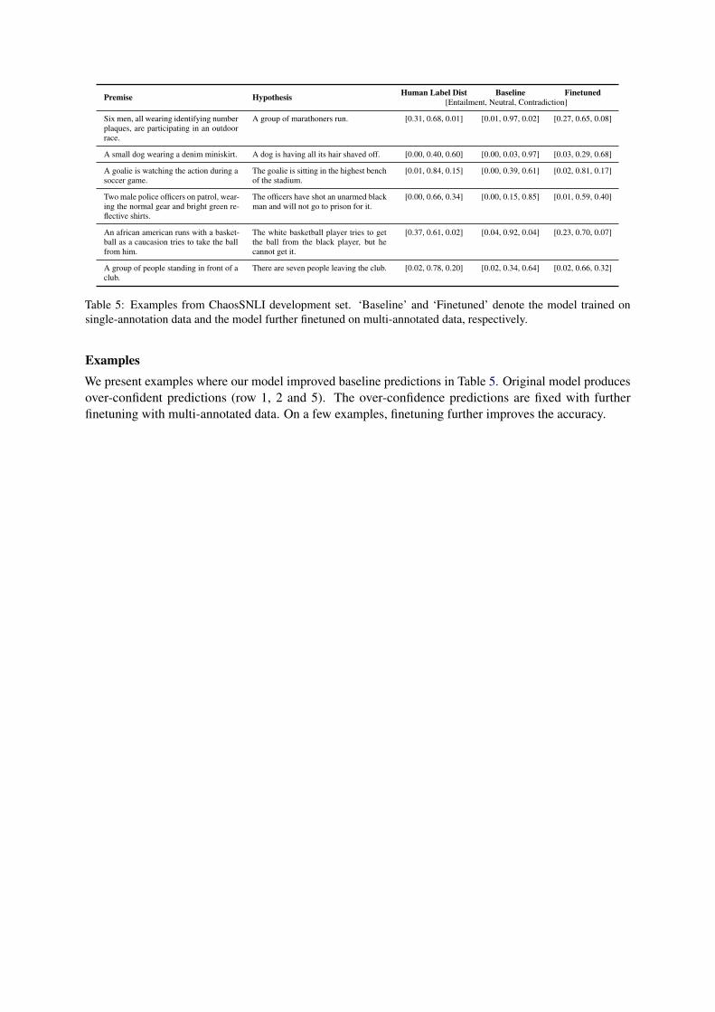
Table 5: Examples from ChaosSNLI development set. ‘Baseline’ and ‘Finetuned’ denote the model trained onsingle-annotation data and the model further finetuned on multi-annotated data, respectively.

ExamplesWe present examples where our model improved baseline predictions in Table 5. Original model producesover-confident predictions (row 1, 2 and 5). The over-confidence predictions are fixed with furtherfinetuning with multi-annotated data. On a few examples, finetuning further improves the accuracy.