capturing risk-premiums in major league baseball...
TRANSCRIPT

Abstract
Capturing Risk-Premiums in Major League Baseball
Contracts An analysis of player variance in performance
and the subsequent effect on player compensation
Joshua Jackson
3/8/2011
Risk premiums are witnessed in many aspects of economics. A risk premium is generally
thought of as the minimum amount of expected return on a risky asset above a risk free asset in
order to justify holding the risky asset. Major League Baseball is a unique setting in which to
study risk premiums. Individual output is well documented and therefore variance in production
for an individual employee is easy to capture. This paper attempts to examine the effect that a
player’s variance in performance has on the compensation he receives. Empirical results from
Major League Baseball using simple OLS Regressions illustrate that only good teams take into
account variance in performance when offering player compensation. Not only do good teams
consider variance in performance when offering compensation, but they actually value risk as a
means to slide up the convex portion of the Major League payoff structure where risk-loving
behavior is promoted.
Jackson 1
Introduction………………………………………………………………………………………………………………………………………………….…………1
Equation 1 ....................................................................................................................................................... 2
Introduction to OPS .................................................................................................................................................. 3
Equation 2 ....................................................................................................................................................... 3
Equation 3 ....................................................................................................................................................... 3
Equation 4 ....................................................................................................................................................... 3
Data…………………………………………………………………………………………………………………………………………………………………………4
Data Collection ........................................................................................................................................................ 4
Data Description ...................................................................................................................................................... 5
Equation 5 ....................................................................................................................................................... 5
Table 1: Summary of Statistics by Contract Length ......................................................................................... 6
Data Breakdown for Analysis .................................................................................................................................. 6
Table 2: Good Teams vs. Bad Teams ............................................................................................................... 9
Table 3: Starters vs. Nonstarters ................................................................................................................... 10
Bias in the Data ...................................................................................................................................................... 10
The Model Specification……………………………………………………………………………………………………………………………….……….13
Equation 6: OLS Regression .......................................................................................................................... 15
Table 4: Variable Definitions ........................................................................................................................ 15
Results…………………………………………………………………………………………………………………………………………………………………..16
Entire Dataset Results.......................................................................................................................................... 16
Regression Results 1: Entire Dataset ........................................................................................................... 18
Good Team Results ............................................................................................................................................. 19
Graph 1: MLB Payoff Table ......................................................................................................................... 20
Regression Results 2: Good Teams…………………………………………………………………………………………………………23
Bad Team Results ................................................................................................................................................ 23
Equations: 7-10 .......................................................................................................................................... 24
Regression Results 3: Bad Teams……………………………………………………………………………………………………………28
Starter Results ..................................................................................................................................................... 28
Regression Results 4: Starters…………………………………………………………………………………………………………..……30
Non-Starters Results ........................................................................................................................................... 30
Regression Results 5: Non-Starters............................................................................................................. 31
Summary……………………………………………………………………………………………………………………………………………………………….33

Jackson 2
Introduction
Major League Baseball (MLB) has always been a valuable setting in which to observe
labor economics. Lawrence Kahn eloquently stated that “there is no research setting other than
sports where we know the name, face, and life history of every production worker and supervisor
in the industry1.” Baseball is a game which is forever intertwined with its almost neurotic
obsession with statistics. These statistics were created as a means to capture an individual’s
contribution to the overall team success. Because of the abundance of relevant statistics and
information on player (employee) performance, it can be expected that owners (employers) will
offer contracts which take into account these performance statistics when compensating players.
Numerous studies have been conducted to identify which offensive statistics most
significantly capture a player’s contribution to a team’s success. David Berri and John Bradbury
constructed an equation aimed at objectively quantifying the amount of runs that a player helps
his team score; the ultimate objective of an offensive player. They used the following equation to
illustrate this idea2:
Equation 1: Runs scored per game =
Berri and Bradbury continued to use performance measures to see which best explained
the variation of runs scored per game. They used batting average, slugging percentage, and on-
base plus slugging percentage (OPS) and found that they explained 65%, 78%, and 89% of the
variation of runs scored per game respectively3. The powerful explanatory value of OPS is the
Jackson 3
reason why I have chosen OPS as my relevant performance statistic when evaluating variation in
player performance and its subsequent effect on player compensation.
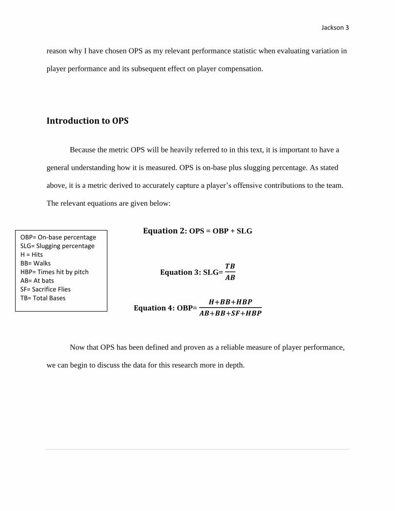
Introduction to OPS
Because the metric OPS will be heavily referred to in this text, it is important to have a
general understanding how it is measured. OPS is on-base plus slugging percentage. As stated
above, it is a metric derived to accurately capture a player’s offensive contributions to the team.
The relevant equations are given below:
Equation 2: OPS = OBP + SLG
Equation 3: SLG=
Equation 4: OBP=
Now that OPS has been defined and proven as a reliable measure of player performance,
we can begin to discuss the data for this research more in depth.
OBP= On-base percentage SLG= Slugging percentage H = Hits BB= Walks HBP= Times hit by pitch AB= At bats SF= Sacrifice Flies TB= Total Bases

Jackson 4
Data
Data Collection
I compiled a dataset taking the skeletal framework of a previous study performed by
Professor Joel Maxcy on the determination of long term labor contracts in Major League
Baseball. I elected to add on to this particular dataset because it had contract information that I
was having trouble locating for more recent years. The dataset included all players’ contract
information who signed a contract between the years 1986 and 1993.
I then added my performance statistics of interest to his dataset. I collected month to
month statistics on all sixteen hundred plus players by hand. I used baseball-reference.com as my
main source for collecting data. The process, while tedious, was not very difficult. The following
steps were used repeatedly throughout the data collection process.
1. Input the players name into baseball-reference.com
2. Open that players monthly splits for the year prior to that player signing a contract (if the
player signed a contract in 1992, the relevant statistical period would be 1991)
3. Input the players monthly performance in OPS, GS, and ABs
4. Repeat this process 1728 times
While I collected a large majority of the data, I did have some degree of help. The UCSD
soccer team (all 25 of them) collected data for about two hours one day. This could lead to
problems with the accuracy and integrity of part of the dataset. To control for this problem, I
personally went back and checked every piece of data that they collected. While this by no
stretch of the imagination insinuates that this is a perfect dataset ‒ with such a tedious process

Jackson 5
there are bound to be mistakes ‒ it does limit the amount of mistakes and thus increases the
accuracy of the dataset and my subsequent findings.
Data Description
The data utilized for this analysis is primarily longitudinal panel data recording contract
information and performance statistics on 1626 Major League Baseball players from 1986-1993.
Each observation contains the players’ statistics from the year prior to signing a contract as well
as other information that was necessary to conducting this research.
The data for each observation can be broken into three specific categories. The first
category is information that can affect the player’s compensation on an individual level outside
of his performance such as arbitration eligibility, free agent eligibility, age, experience, defensive
position, and year signed.
The second category is the player’s performance statistics which were gathered to
calculate offensive contributions to the team. These statistics include OPS, OPS by month, at
bats, games started by month, games started for the season, and our “risk” measurement of OPS
variance. OPS variance is calculated in the traditional manner of variance by simply taking
deviations from the mean squared and dividing by the number of observations as shown by
Equation 5.
Equation 5: ∑
Jackson 6
The third and final category of data that was collected was team level data. This included
the team that signed the player, the opening day payroll of that team, that teams previous year
win total, and the amount of wins that team was away from 95 wins.
Of these 1626 observations, there were 1341 one year contracts and 285 long term
contracts. A more detailed account of the contract type with relevant information is shown in
table 1 below.
Table 1: Summary of Statistics by Contract Length
1 Year Contract
2 Year Contract
3 Year Contract
4 Year Contract
5 Year Contract
6 Year Contract
Total
Number of Observations
103 1 1626
Mean OPS .770 1.08 .706
St. Dev. OPS .098 Na .1136
Mean OPSVAR
.0165 .0282 .0291
St. Dev. OPSVAR
.0141 Na .0502
Mean EXP 7.27 7 5.43
Mean Age 29.7 28 28.58
Mean GS 131.33 138 90.52
Data Breakdown for Analysis
Along with simply running a regression over the entire dataset, I have also decided to
decompose the data and run similar regressions over these sub-datasets. The first way in which
the data was broken down was by the amount of wins the team recorded during the previous
Jackson 7
year. I decided to do this because it is entirely possible that good teams view variance in a
significantly different manner than bad teams. It is my hypothesis that “good teams” are likely to
value low variance type players while “bad teams” are more likely to value high variance type
players.
I believe that good teams will value low variance type players because they already have
a high previous year win total. If a team is already successful, it is unlikely that they would value
a player that will provide uneven contribution to the club. They would prefer to sign a player
who has a low variance in performance and can help the good team continue their winning ways.
Risk is not something that a good team needs to add because they have proven that they can win
as the team is currently built. Adding unnecessary risk is not a proposition that a good team
should favor.
Bad teams might take a different approach to evaluating variance in performance. In
baseball, there is little difference between losing 100 games and 110 games. Either way, your
team is probably in last place in your division. This general rule is why I hypothesize that bad
teams will greatly value variance in performance when signing players.
Bad teams employ a strategy which I will call the “Hail Mary” approach (different sport
same idea). Bad teams will want to sign as many high variance players as they can. They should
do this for two reasons. First, high variance players should be cheaper if my initial hypothesis for
how good teams should act in player bargaining holds. Because good teams do not target these
kinds of players, their market value should be lowered. Bad teams could sign these players at a
discount because there is less competition in the market for high variance type players.
Second, if a few of these high variance type players happen to perform at their highest
percentile for an extended period of time, the bad team might have a chance of winning their
Jackson 8
division, making the playoffs, and even winning the world series. Using this logic, bad teams
look to sign as many high variance type contracts as possible because they know that is their
only way of competing. And what if these players all perform at their lowest percentile and end
up making the team worse? Well, the bad team loses a few more games than they did before and
miss the playoffs by 25 games instead of 20. With these high variance type players, bad teams at
least have a shot at winning. This low-risk medium-reward strategy is what I believe will
incentivize bad teams to value high variance type players.
One interesting case might be if a good team loses many of its good players from the
previous year. A good team that has multiple star players eligible for arbitration or free agency
might not be able to retain them given certain payroll constraints. If a good club loses many of its
key impact players, they might act as a bad team in their valuation of variance even if they had a
high win total from the previous year. A good team, as defined from previous year wins,
valuating risk as a bad team might be occasionally observed for this reason. However, I believe
that my original hypothesis, that good teams will dislike variation in performance while bad
teams will prefer it, can be proven correct despite admitted exceptions.
Good teams and bad teams were separated by how many wins away they were from the
average amount of wins needed to make the playoffs during this time period. The average
number of wins needed to make the playoffs was calculated to be right around 95 games. Thus, if
a team was within 15 games of making the playoffs the previous season, they were considered a
good team. If they were not within 15 games of making the playoffs, they were classified as a
bad team.
This classification of good and bad teams is problematic in that you lose explanatory
value when binary classifications are made. There are obvious differences between the 1988
Jackson 9
Braves who won 54 games and were -41 games away from 95 wins and the 1986 Cardinals who
won 79 games and were -16 games away from 95 wins. However, this way is sufficient in
differentiating good and bad teams so that their differing views on variance in performance can
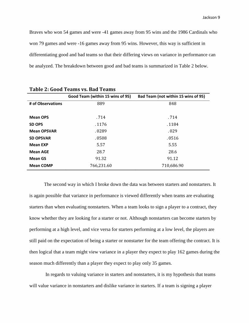
be analyzed. The breakdown between good and bad teams is summarized in Table 2 below.
Table 2: Good Teams vs. Bad Teams
Good Team (within 15 wins of 95) Bad Team (not within 15 wins of 95)
# of Observations
Mean OPS
SD OPS
Mean OPSVAR
SD OPSVAR
Mean EXP
Mean AGE
Mean GS
Mean COMP
The second way in which I broke down the data was between starters and nonstarters. It
is again possible that variance in performance is viewed differently when teams are evaluating
starters than when evaluating nonstarters. When a team looks to sign a player to a contract, they
know whether they are looking for a starter or not. Although nonstarters can become starters by
performing at a high level, and vice versa for starters performing at a low level, the players are
still paid on the expectation of being a starter or nonstarter for the team offering the contract. It is
then logical that a team might view variance in a player they expect to play 162 games during the
season much differently than a player they expect to play only 35 games.
In regards to valuing variance in starters and nonstarters, it is my hypothesis that teams
will value variance in nonstarters and dislike variance in starters. If a team is signing a player

Jackson 10
they expect to be a substantial contributor on an every game basis, they might pay for a little
more certainty about their offensive output. For nonstarters, a team might prefer a player with
high variance because they are not expected to be everyday contributors. The coach can put in
these types of players when they need an extraordinary performance that he believes a high
variance type player might be able to deliver.
Table 3: Starters vs. Nonstarters
Starters (started at least 130 games) Nonstarters (started fewer than 130 games)
# of Observations
Mean OPS
SD OPS
Mean OPSVAR
SD OPSVAR
Mean EXP
Mean AGE
Mean COMP
Bias in the Data
For the subsequent discussion of bias captured by the dataset, it is important to
understand that much of the analysis will be taken from Joel Maxcy’s original research. Because
the contract data which I am utilizing is the same data collected by Maxcy years before, the same
bias which his collection introduced into the system will still exist. A brief summary of his
analysis of these biases is the basis of the following two paragraphs.
The amount of times that a player is represented in this dataset varies based on the
number of contracts a player signed during this particular time period. Many players signed
multiple contracts of varying lengths during our years of interest while some only signed one
Jackson 11
contract. This can be because of many reasons, but for our purposes, understanding that some
players are represented in this dataset more than once is sufficient4.
The contract data also contains some selection bias because it is possible that some
contract terms went unreported. Thus, those that were not reported would not be included in the
dataset. This problem obviously makes the dataset neither comprehensive nor random. Most
common in these omissions are players which did not hold a major league contract but played
with the club for all or part of the season. Also missing from the data might be veteran players
who elected to sign unreported extensions rather than new contracts. Signing an unreported
multi-year extension, akin to signing a multi-year contract, could lead to observations being
omitted5.
Other biases pertaining to my added performance statistics outside of the contract data
collected by Maxcy also exist. It is outside of the realm of this dataset to account for a player
whose statistics were hampered due to an injury. Teams at the time of signing would have a
better understanding of whether or not a player’s injuries were the cause of his low output. If
teams believe that a player’s low output could have been caused by a minor injury that should
heal, the team might sign the player to a larger contract than his injury impaired statistics justify.
Another situation which cannot be accounted for within my dataset is minor league
players who are mid-season call ups. This would result in fewer observations of monthly splits
for younger players and thus increase their variance in OPS simply by decreasing the number of
monthly observations.
Also relevant to this study is the convicted collusion of the MLB owners from 1986-
1988. Owners colluded against free agents during this time period to keep the price of star
players down6. This resulted in a negative shock on compensation that was unrelated to a decline
Jackson 12
in performance. To control for this, a dummy variable YR1989 was created for all contracts that
were signed between 1986 and 1989.
Some players were dropped from the study for a variety of reasons. The main reasons for
dropping players were the absence of performance statistics for the relevant time period and if
the player was a pitcher.
This dataset contains only offensive players. Pitchers were not included in this study
because their contribution to the team is measured much differently than position players.
Pitchers are not compensated based on their offensive production but rather their ability to get
opposing players out.
The final bias that exists in the data is probably the most important as it relates to this
study specifically. I evaluate variance in performance over a six month sample with one
observation each month. However, to obtain a high variance in performance, a player must be
capable of performing extremely well for some period of time. For example, a player that has a
low variance in performance might have monthly splits in OPS of .500, .550, .525, .530, .550,
and .525 over the six month season. This is a below average player. He is very consistent, but he
is consistently below average.
Contrast this with a player who might have high variance in performance. This player
might have monthly splits in OPS that are .900, 1.240, .560, .675, .800, and .950. He has a higher
OPS in every month than our theoretically consistent player. Thus, he should be expected to be
paid substantially more despite his perceived inconsistency. Because I am unable to distinguish
between these two situations, it could cause the regressions to overvalue variance in performance
in player compensation because it is capturing the player’s ability to obtain a high OPS rather
than how teams view his variance in performance.

Jackson 13
I believe that the above scenario should not arise very often and should be mitigated by
another scenario that will lead to an undervaluation of OPS variance. A player could have the
same OPS statistics as our second hypothetical high variance type player but with a very low
number of at-bats. The low number of at-bats might be the reason for a poor player posting a
very high OPS during a certain month. The poor player might only get 4 at-bats one month, hit a
home run and post an OPS of 1.250. This is obviously different from a very good player
attaining such an OPS over 120 at-bats during a given month. Because a team can observe that
the player getting fewer at-bats could have been lucky, he would not be compensated as a player
capable of posting such a high OPS. This scenario, which could cause OPS variance to be
undervalued, should work to offset the original circumstance which overvalued variance in OPS.
Finally, the inclusion of OPS in the regression itself should help control for these types of
situations.
The Model Specification
The model used to test the significance of the data will be a simple Ordinary Least
Squares regression (OLS). One of the major biases I expect within the framework of an OLS
regression for this study is the fact that not all teams have perfect information about a player
outside of his statistics. For example, a player might have subpar performance statistics but be
paid a higher compensation by his current team because of his intangible value to the club. These
types of positive externalities that a single player might have on his team are something which is
unobservable in the data and to other clubs who are bidding on that player.

Jackson 14
While it might be fair to assume that during the time of bidding, other clubs had a general
understanding of what “intangibles” a player might bring to their team, it is obvious that this is a
market in which perfect information is not available to all parties. In hopes of partially correcting
for this problem, I will use a variable found in Maxcy’s original dataset known as SWITCH. This
is a dummy variable coded 1 if the player switched teams when he signed his contract and 0
otherwise. This should control for some of the compensation given to a player because of
information that is unavailable to all bidders.
The opposite case can also be true. A team might have information about a player on
their current roster that is a negative externality to the team for a variety of reasons. The
SWITCH dummy is used to control for this problem as well. The regression utilized during this
study is given in Equation 6 on the next page.

Jackson 15
Equation 6: OLS Regression
Table 4: Variable Definitions
Variable Definition
OPS_VAR Variance in monthly OPS over the season prior to signing the new contract
VARGS Interaction term between OPS_VAR and GS_SEASON
VARWIN95 Interaction term between OPS_VAR and Wins_From_95
WINS_FROM_95 Amount of wins the team was from 95 the year prior to signing the player
EXP Years of experience the player has in the league when contract was signed
AGE Players age as of June 1st of the year he signed his contract
SWITCH Dummy variable if the player switched teams is 1, 0 if otherwise
OPEN_PYRL Opening day payroll of the team for the year that they signed the player
OPS Season on-base plus slugging percentage
GS_SEASON Games started for the season the year prior to signing the contract
AE1 Dummy variable coded 1 for the 1st year of arbitration eligibility, 0 otherwise
AE2 Dummy variable coded 1 for 2nd
year of arbitration eligibility, 0 otherwise
AE3 Dummy variable coded 1 for 3rd
year of arbitration eligibility, 0 otherwise
FA Dummy variable coded 1 if free agent eligible, 0 otherwise
YR1989 Dummy variable coded 1 if the contract signed between 1986-1989, 0 otherwise
C Dummy variable coded 1 if the players primary position is catcher, 0 otherwise
SS Dummy variable coded 1 if the players primary position is shortstop, 0 otherwise
COMP Compensation in terms of dollars per year as stated in his contract
Jackson 16
Results
Entire Dataset
The initial regression involving the entire dataset shows that variance in performance is
not significant in determining compensation if the data for the league is taken as a whole. The
results table of Regression 1 can be found at the end of this section.
Owner collusion, represented by the variable YR1989, showed that players who signed
contracts between the years 1986 and 1989 could expect to earn substantially less than if they
had not signed during this time period. Switching teams also had a negative relationship towards
player compensation. This is probably because of the incomplete information that the bidding
teams have about a player not currently on their roster. Teams do not want to offer as much
money for a player who they have questions or concerns about.
Age is also negative which speaks to the expected career arc of a Major League player.
Players are expected to hit their primes somewhere between the ages of 26 and 32. A players
performance plotted against age would look like an inverse parabola. A player’s peak earning
years should be during his prime and then taper off from there.
Opening day payroll has a positive effect on player compensation. This is to be expected
that higher revenue grossing teams can afford to spend more on targeted players. Our
performance statistic OPS is the most impactful coefficient on player compensation. Players are
paid for their offensive contribution to the team. Because OPS is an accurate measure capturing
this contribution, the coefficient should be significant and positive.

Jackson 17
Games started the previous season have a positive effect and a high level of significance.
Again, this is an expected finding. Players that started games the previous season should
command a higher salary than those who did not.
All three of our arbitration eligibility measures are significant. This is because the player
is gaining more bargaining power and essentially eroding the restrictive monopsony power held
by clubs7. By the time a player hits free agent eligibility, the monopsony power of clubs has been
wiped away completely.
While it might seem shocking that experience is insignificant in this regression, the above
paragraph reveals why. The main reason why experience should be positively correlated with a
higher salary is because of the increased negotiating power that the player obtains by accruing
years of service in the league. Obtaining arbitration eligibility and free agency both increase the
player’s ability to openly negotiate with other teams and increases his market value. The positive
effect that experience would have on compensation is absorbed by the inclusion of the different
arbitration levels and free agency.

Jackson 18
Regression Results 1: Entire Dataset
Variable Name Reg 1.1 Reg 1.2 Reg 1.3 ops_var 168578.92
(342727.91) 145195.76
(562954.13) 583679.74
(628188.98) YR1989 -158245.61***
(44031.801) -158387.48***
(44128.692) -155057.47***
(44159.561) switch -88690.911
(45828.114) -88827.795 (45916.785)
-83988.377 (45999.26)
exp 6107.9036 (10905.213)
6128.4644 (10915.657)
6720.5517 (10917.202)
age -21332.61* (8699.0153)
-21336.774* (8702.0756)
-21905.25* (8705.6459)
open_pyrl 0.0271339*** (0.00198067)
0.0271326*** (0.00198144)
0.02717428*** (0.00198072)
wins_from_95 -2554.7482 (1662.9159)
-2509.7287 (1872.4497)
-2427.0596 (1872.3376)
ops 1695374.3*** (173441.15)
1695545.7*** (173525.82)
1723413.1*** (174352.56)
gs_season 6567.8374*** (462.76903)
6567.1249*** (463.11243)
6810.6177*** (488.18852)
ae1 199025.99*** (54805.423)
199012.36*** (54823.034)
200925.61*** (54811.62)
ae2 585701.43*** (59686.22)
585609.51*** (59730.526)
586819.91*** (59708.308)
ae3 767580.67*** (69380.236)
767438.21*** (69455.038)
769178.65*** (69432.265)
Fa 881971.59*** (83788.287)
881795.21*** (83881.915)
879377.32*** (83857.865)
C 14906.535 (46846.67)
14945.645 (46867.146)
17047.224 (46864.926)
ss -849.85551 (60427.695)
-996.41494 (60511.185)
-3043.4694 (60497.685)
nl 21747.184 (33176.541)
21739.878 (33187.121)
23527.075 (33191.535)
VarWin95 -1565.488 (29894.382)
-7439.8608 (30114.093)
VarGS -16637.466 (10596.441)
_cons -1401875.3*** (253771.22)
-1401075.5*** (254308.91)
-1413666.5*** (254319.59)
*=.05 significance level **=.01 significance level ***=.001 significance level

Jackson 19
Good Team Results
Breaking down the data into two sub-datasets containing good teams and bad teams has
yielded very interesting results that contradict my initial hypotheses. Regression 2.1 (which can
be found at the end of the chapter) shows that when a regression was run on the dataset
containing only good teams, the variance in performance measure (OPS_VAR) was large and
significant at the 5% level. Not only is OPS_VAR large, it is large and positive. This evidence
starkly contradicts my original hypothesis that good teams will devalue a player if they have a
high variance in performance. Because these results were in direct contradiction with my original
hypothesis, I will attempt to offer an explanation as to why we are witnessing good teams paying
for OPS_VAR.
I believe that we are witnessing this risk-loving behavior because the payoff table for a
MLB club is convex. Payoff is generally defined here as an all-encompassing capture of any
benefit to the club (who is offering the contract) for winning. This includes increased attendance
at the ballpark, explicit financial rewards for making the playoffs and winning the World Series,
and job security for the front office that puts together a winning team. When analyzed in this
manner, it is not a significant assumption to view the MLB payoff structure as an exponentially
increasing payoff table that culminates in a World Series victory.
Because of the convex nature of the MLB payoff table, teams should employ a risk-
loving strategy. The return on the investment for a player with a high variance can possibly be
enormous because of the shape of the MLB payoff table.
A graphical representation of this theoretical analysis can be found in Graph 1 below.
Looking at the graph, a 5 win increase for the Yankees or Dodgers will provide a large increase
in their payoffs because of the exponentially increasing nature of the payoff table. Compare the

Jackson 20
potential gains of a 5 win increase with the potential losses of a 5 win decrease (if the high
variance player does not perform). Gains obtained by sliding up the payoff curve will always
outweigh the losses realized from sliding down the payoff curve by the same amount. Because of
the convexity of the payoff table, the rewards outweigh the risk.
This can be mathematically understood using simple derivatives. If you are at a certain
point on an increasing function,
towards the increasing region of the function (to the right in
Graph 1) is always greater than
towards the decreasing region (to the left in Graph 1). This is
why good teams are not only willing to bring on a player who displays a higher variance in
performance, but they actually target these types of players.
Graph 1: MLB Payoff Table
The interaction term VarGS representing the interaction between OPS_VAR and
GS_SEASON represents the idea that good teams view variance in performance differently
Jackson 21
depending on how many games the player started the previous year. The effect is small and
negative implying that the more games a player started the less variance a good team would like
out of that player. Although the effect is rather small, this illustrates that good teams would like
their starters to be more consistent than their bench players.
There were no meaningful changes in the level of significance reached or the coefficient
magnitude for the variables that were also included in Regression 1. I expect many core
variables ‒ YR1989, age, open_pyrl, wins_from_95, ops, gs_season, ae1, ae2, ae3, and fa ‒ to
more or less remain significant throughout all regressions.
In regression 2.2 I decided to add the term wins_from_95. As might be expected, the
introduction of this term did not change the size or significance of any other variables. The
dataset is already broken down into good and bad teams so adding a variable controlling for wins
should have little effect.

Jackson 22
Regression Results 2: Good teams
Variables Reg 2.1 Reg 2.2
ops_var 1143581.4* (575312.4)
1143677.7* (575838.39)
VarGS -37426.287* (15206.633)
-37430.317* (15228.314)
YR1989 -138088.57* (59062.933)
-138032.28* (59744.005)
switch -47157.809 (61134.185)
-47182.246 (61287.658)
exp 5369.096 (14328.341)
5370.6768 (14338.679)
age -30234.144* (12138.271)
-30236.046* (12148.854)
open_pyrl 0.02828477*** (0.00265966)
0.02828838*** (0.0027199)
ops 1446504*** (224368.79)
1446560.2*** (224668.27)
gs_season 7534.9509*** (637.89914)
7534.9128*** (638.29287)
ae1 239170.51*** (71387.433)
239183.04*** (71455.049)
ae2 722092.14*** (78557.329)
722100.41*** (78612.97)
ae3 862932.21*** (91343.428)
862944.68*** (91416.509)
fa 923692.86*** (109739.1)
923722.85*** (109901.49)
c 10763.405 (60526.228)
10762.451 (60561.144)
ss -125905.65 (81457.424)
-125897.24 (81514.691)
nl 74954.686 (43433.842)
74962.404 (43475.4)
Wins_from_95 -24.257964 (3779.6304)
_cons -1096128.4** (349879.75)
-1096377.4** (352223.01)
*=.05 significance level **=.01 significance level ***=.001 significance level

Jackson 23
Bad Team Results
The same regressions that were run utilizing the good team dataset were subsequently run
on the bad team dataset and the results are shown in the Regression 3 results table at the end of
the chapter. Many variables which were significant in the determination of compensation for
good teams are insignificant for bad teams.
Our main variable of interest, OPS_VAR, is now insignificant. The fact that OPS_VAR
is insignificant for bad teams neither rejects nor confirms my initial hypothesis that bad teams
should value risk in some type of “Hail Mary” strategy. However, it is problematic for my above
analysis about the convexity of the MLB payoff table. If the MLB payoff structure is indeed
convex, then all teams, regardless of initial placement, should employ risk-loving behavior.
For example, let us refer back to Graph 1 and see what happens if the Brewers see a 5
win increase (the same size increase as for the Yankees and Dodgers in the good team analysis).
This increase will not realize an impressive increase in pay off because of their position on the
payoff curve. However, a 5 win decrease does not lose the Brewers very much payoff either. The
rewards of taking on a high variance type player seem to outweigh the risk even for teams on the
lower end of the payoff table. So why don’t the regressions show that the bad teams value
variation in performance? If the payoff structure of Major League Baseball is in fact convex,
then shouldn’t all clubs take on a risk-loving strategy?
I believe that the answer to the above question is not necessarily. Decisions between how
good and bad teams value variance are not made in a vacuum. The good teams will target high
variance type players, as shown in regression 2. By targeting these players, good teams drive up
the price of the high variance type player. Not only do they drive up that player’s price, but
because of their current location on the MLB payoff table, their expected reward of signing that

Jackson 24
player is strictly greater than the expected payoff of a bad team signing the same player. Because
their expected reward is greater, good teams should theoretically pay strictly more for a high
variance type player than a bad team. Many of the high variance type players are absorbed by the
good teams for larger contracts. This is illustrated mathematically below.
Equations: 7-10
(7) ;
(8)
(9)
(10)
The above equations are an attempt to explain why a risk-loving strategy might not be
observed by bad teams despite the convex nature of the MLB payoff curve. In order to complete
the analysis, it should be assumed that both the good team and the bad team want player X
equally. Also, they will both offer the max contract which they are capable of offering to player
X.
Equation 7 shows the fair equilibrium of a contract in this case. The compensation
offered to the player by a club should be equal to the expected value that player will bring to the
club. Equation 8 shows that because of the difference in position on the convex MLB payoff
curve, good teams have an expected payoff from signing player X that is greater than or equal to
the bad team’s expected payoff. If this statement is true, then equation 9 is also true. The
𝑬 𝝓 𝑮𝒐𝒐𝒅= Good teams expected payoff of signing player X
𝑬 𝝓 𝑩𝒂𝒅= Bad teams expected payoff of signing player X
𝜸𝑮𝒐𝒐𝒅= Good teams compensation offer to player X
𝜸𝑩𝒂𝒅= Bad teams compensation offer to Player X
Jackson 25
compensation offered by a good team to Player X should be greater than or equal to the
compensation offered by a bad team. Because a good team can justify offering more money to
Player X than a bad team, we can end up at a situation like Equation 10. Equation 10 shows that,
assuming our previous equations and assumptions hold, the highest compensation offered to
Player X by a good team will always be greater than the expected return that a bad team can
expect for signing that player (assuming both teams offer the max amount they are capable of
offering). In this circumstance, a bad team will obviously choose not to pursue the high variance
type player. They have essentially been priced out by the better teams.
Following the same iterative logic as provided above, the opposite case can never be true.
Bad teams highest contract offer can never be higher than a good teams highest contract offer.
This is why we can see risk-loving behavior from the top portion of our convex curve and not
from the bottom portion.
It should be understood that the above analysis offers a general theory as to why we
might witness good teams targeting variance while bad teams do not despite the convexity of the
MLB payoff curve. I am not attempting to prove any type of general equilibrium for contract
negotiations. There are many other factors that go into offering a player a contract as shown by
the multiple regressions I have run. I am offering a theory as to why bad teams might not employ
a high-risk strategy despite the fact that the convexity of the MLB payoff table promotes risk-
loving behavior regardless of current position.
The interaction term between variance and games started (VarGS) has also lost its
significance. If our variance term has lost significance, it makes sense that its interaction terms
involving variance will also lose significance.
Jackson 26
The dummy variable SWITCH has now become significant at the 5% level in a large and
negative way. This large negative effect probably captures efforts by bad teams to build from
within their farm system. Teams that are out of contention often look to rebuild within their
organization by using cheap players that were recently drafted and are still on their rookie
contracts. They purge their current roster in order to make room for these cheaper and usually
younger players. Signing or retaining major league tested players is too expensive for a team that
has little hope of competing. Instead, they usually choose to build for the future through players
who are both cheap and young.
Two of our previously coined “core variables” have lost their significance. Age and AE1
are now insignificant in Regression 3.1. Age and AE1’s decline can possibly be explained by bad
team’s propensity to purge their roster and build from within the organization. They do not want
to retain bad players at a higher cost so they would rather use young talent on minor league
rosters to fill out their team.
Regression 3.2 shows that the introduction of the variable wins_from_95 has no effect on
the original results obtained from Regression 3.1. Only the variable SWITCH, which barely
made the cut off for significance at the 5% level (t-test was -1.96), lost its significance.

Jackson 27
Regression Results 3: Bad Teams
Variable Reg 3.1 Reg 3.2
ops_var 88243.391 (838693.25)
101481.26 (839962.75)
VarGS 2352.846 (15638.434)
2115.9988 (15660.974)
YR1989 -190206.57** (65642.698)
-195610.06** (67293.669)
switch -136898.47* (69746.348)
-135822.31 (69849.095)
exp 13041.358 (16786.834)
12624.493 (16834.836)
age -18953.131 (12598.289)
-18983.821 (12606.127)
open_pyrl 0.02524362*** (0.00289054)
0.02497204*** (0.00298439)
ops 2059911.1*** (276837.58)
2057606.5*** (277074.14)
gs_season 5771.6106*** (758.76227)
5781.9053*** (759.7299)
ae1 149980.12 (85000.456)
150186.26 (85053.321)
ae2 435529.04*** (91681.382)
438794.45*** (92161.991)
ae3 666635.96*** (106402.12)
665130.71*** (106544.07)
Fa 859806.15*** (129363.34)
863598.97*** (129848.21)
C 27649.92 (73486.549)
28736.428 (73589.561)
Ss 100596.01 (90755.388)
101472.62 (90840.924)
Nl -35777.608 (51604.404)
-34807.433 (51702.237)
wins_from_95 1653.5683 (4479.7866)
_cons -1504357.6*** (363363.58)
-1457326.6*** (385261.15)
*=.05 significance level **=.01 significance level ***=.001 significance level

Jackson 28
Starter Results
The results on the sub-dataset containing only starters are provided on the next page. The
results for starters are fairly ambiguous and do little to help confirm or deny my hypothesis that
teams will dislike variance in starters and value variance in non-starters.
One interesting finding with regards to the starters dataset is the wins_from_95 variable.
Wins_from_95 has a significant negative effect on the compensation of a starter. This was a
variable which has been insignificant in all of the previous regressions. The further a team is
away from 95 wins, the further that team is away from the playoffs. Because this type of team
probably expects to be more than a few starters away from making a major jump in win total,
they would rather not pay for a starter to come make their team marginally better. Instead, they
would like to rebuild their team from within their own farm system (as previously discussed) and
sign the final pieces when they have a better team. This process possibly accounts for the
significant negative relationship between wins_from_95 and compensation of starters.

Jackson 29
Regression Results 4: Starters
Variable reg4_1
ops_var -4057245.9 (6059790.6)
VarWin95 139984.56 (382765.86)
YR1989 -297281.83** (108776.13)
switch -25019.992 (132856.52)
exp -4458.8753 (29533.01)
age -38618.393 (26940.397)
open_pyrl 0.0558645*** (0.00485201)
wins_from_95 -15527.552* (6794.4923)
ops 4372161.9*** (501243.96)
gs_season 15690.717** (4801.0644)
ae1 559917.7*** (125789.98)
ae2 1105824.3*** (137047.15)
ae3 1494553.2*** (152971.73)
Fa 1694621.7*** (214390.9)
C -65003.93 (210841.84)
Ss 74907.178 (127036.19)
nl 17243.273 (79784.051)
_cons -5169102.6*** (1035462.5)
*=.05 significance level **=.01 significance level ***=.001 significance level

Jackson 30
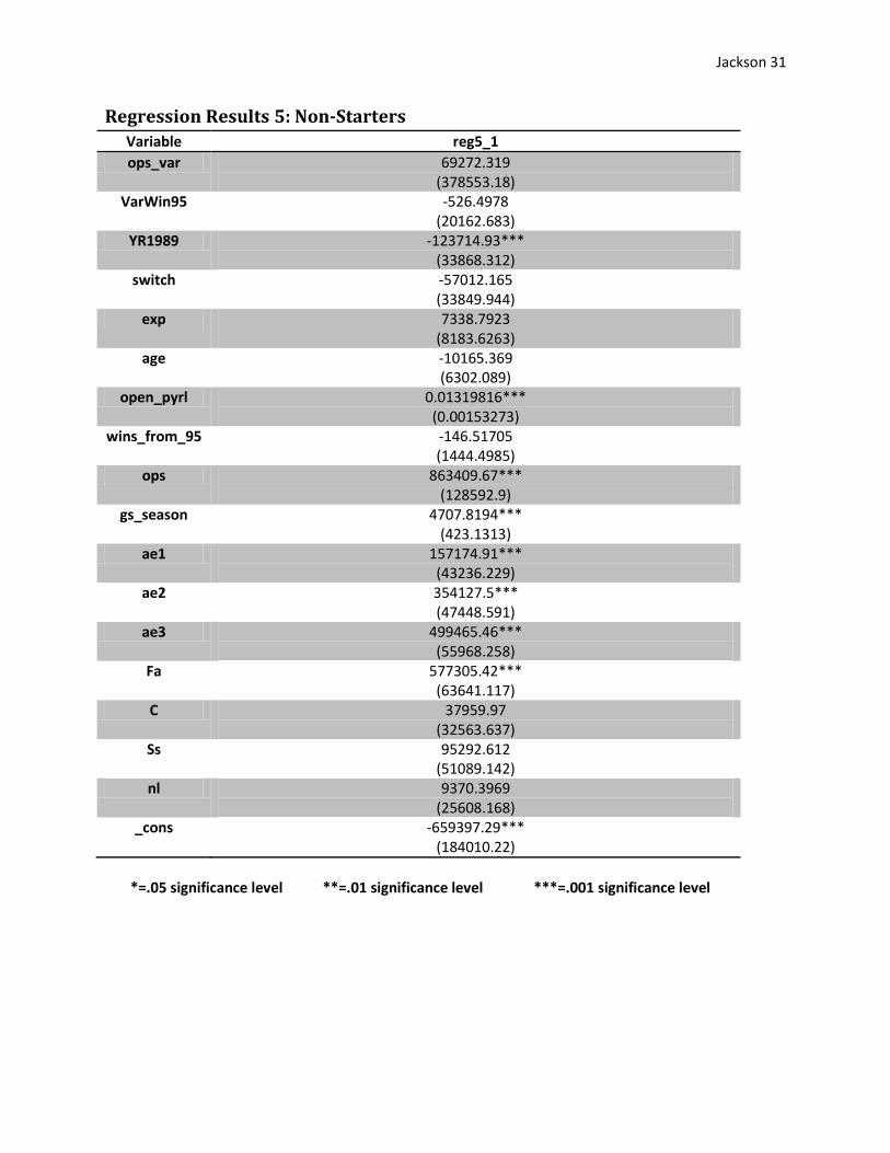
Non-Starters Results
The regression run over the non-starter dataset also neither confirms nor denies my
original hypothesis with regards to starters and non-starters. The variables which held
significance in the starters’ regression also held significance in the non-starters’ regression with
one exception: wins_from_95.
Not only did wins_from_95 become insignificant, the standard error is ten times larger
than the actual coefficient. A team’s win total from the previous year does not seem to influence
the compensation of a non-starter. A possible reason could be because the market for non-starters
is not as competitive. Bad teams are able to sign non-starters at market value even though they
are rebuilding because their market value is relatively cheap.
Jackson 31
Regression Results 5: Non-Starters
Variable reg5_1
ops_var 69272.319 (378553.18)
VarWin95 -526.4978 (20162.683)
YR1989 -123714.93*** (33868.312)
switch -57012.165 (33849.944)
exp 7338.7923 (8183.6263)
age -10165.369 (6302.089)
open_pyrl 0.01319816*** (0.00153273)
wins_from_95 -146.51705 (1444.4985)
ops 863409.67*** (128592.9)
gs_season 4707.8194*** (423.1313)
ae1 157174.91*** (43236.229)
ae2 354127.5*** (47448.591)
ae3 499465.46*** (55968.258)
Fa 577305.42*** (63641.117)
C 37959.97 (32563.637)
Ss 95292.612 (51089.142)
nl 9370.3969 (25608.168)
_cons -659397.29*** (184010.22)
*=.05 significance level **=.01 significance level ***=.001 significance level

Jackson 32
Summary
Although almost all of my original hypotheses were either inconclusive or completely
wrong, this paper still has provided many interesting results. In this paper, I attempted to capture
how variance in performance is evaluated by Major League Baseball teams. Through the
regressions, it can be seen that risk is evaluated differently depending on certain factors such as
team and individual success. Because of the increasing nature of the MLB payoff structure, good
teams take on a risk-loving strategy that essentially prices out the bad teams. However, there is
little evidence to suggest that variance is a significant factor in determining compensation
between starters and non-starters.
Further research would be interesting and necessary to truly capture variance in
performance and its subsequent effect on player compensation. A similar study using more
recent data would be interesting for multiple reasons. First, the payoff structure of Major League
Baseball has undoubtedly changed over the years. Eight teams make the playoffs under the
current format as opposed to four during the time period of this study. Also, baseball has grown
into a multi-billion dollar globalized industry. The expected increase in payoffs from making the
playoffs and winning the World Series are possibly greater in today’s game than they used to be.
Secondly, revenue sharing might have skewed the payoff structure of Major League
Baseball so that it is in a low-revenue team’s best interest to continue with a low payroll even if
signing a high profile player can increase their win total. It is possible that this would create
some type of parabolic payoff structure that causes teams to try to get to either end of the payoff
structure because the value in this type of situation should be at the margins. It would be perverse
if revenue sharing, a policy implemented to subsidize the payroll of small market teams, actually
incentivizes teams to take on even less payroll. A study examining the effect of revenue sharing
Jackson 33
on the MLB payoff structure and its subsequent effect on player compensation would be very
interesting.
The third thing that has changed in baseball today is the typical contract structure. More
and more long-term guaranteed contracts are now being given to players. Players routinely sign
for six years and one hundred million dollars in 2010. These types of numbers were unheard of
between 1986 and 1993.
The fourth thing that has evolved during twenty-first century baseball is the use of
advanced metrics to evaluate player performance. While OPS is still a highly valuable statistic,
new stats such as wins above replacement (wins added by an individual player to a team),
ultimate zone rating (a defensive metric), and batting average on balls in play (a metric used to
assess the luck of a player) might be valuable metrics to consider when conducting a future study
on variance in performance.
A final problem which I believe a future study could improve upon is my inability to
distinguish “good variance” from “bad variance”. As discussed in the bias section, in order to
have a high variance in performance, the player must be good enough to achieve a high OPS
over some period of time. In contrast, some players are lucky to achieve such an OPS over a
small sample. Extracting the difference in these types of variances could be very interesting to
work with in the future. However, I was unable to identify this type of variance and thus
eliminate the bias that coincides with this problem.
I believe that this paper is a first step into capturing how teams evaluate variance in
performance when signing players to Major League contracts. It is hard to believe that few
people have ever tried to capture a risk-premium in this way before. It is a difficult undertaking

Jackson 34
and a flawless method might be years away, but the research must start somewhere and I believe
that this research is a significant step in the right direction.
Appendix
1 Kahn, Lawrence M. "Free Agency, Long-Term Contracts and Compensation in Major League Baseball: Estimates
from Panel Data." Review of Economics and Statistics 75.1 (1993): 157-64. JSTOR. The MIT Press. Web. 2 Berri, David J., and John C. Bradbury. "Working in the Land of Metricians." Journal of Sports Economics 11.1
(2010): 29-47. Print. 3 Berri, David J., and John C. Bradbury. "Working in the Land of Metricians." Journal of Sports Economics 11.1
(2010): 29-47. Print. 4 Maxcy, Joel. "Motivating Long-Term Employment Contract: Risk Management in Major League Baseball."
Managerial and Decision Economics 25.2 (2004): 109-20. Print. 5 Maxcy, Joel. "Motivating Long-Term Employment Contract: Risk Management in Major League Baseball."
Managerial and Decision Economics 25.2 (2004): 109-20. Print. 6 Zimbalist, Andrew S. Baseball and Billions: a Probing Look inside the Big Business of Our National Pastime. New
York, NY: Basic, 1994. Print. 7 Maxcy, Joel. "Motivating Long-Term Employment Contract: Risk Management in Major League Baseball."
Managerial and Decision Economics 25.2 (2004): 109-20. Print.