Capturing the Dynamical Repertoire of Single Neuronswith Generalized Linear ModelsAlison I. Weber1 & Jonathan W. Pillow2,3

1Graduate Program in Neuroscience, University of Washington, Seattle, WA, USA.2Princeton Neuroscience Institute, Princeton University, Princeton, NJ, USA.3Dept. of Psychology, Princeton University, Princeton, NJ, USA.

Keywords: point process; generalized linear model (GLM); Izhikevich model; spike timing;variability

Abstract

A key problem in computational neuroscience is to find simple, tractable models that are never-theless flexible enough to capture the response properties of real neurons. Here we examinethe capabilities of recurrent point process models known as Poisson generalized linear models(GLMs). These models are defined by a set of linear filters, a point nonlinearity, and condi-tionally Poisson spiking. They have desirable statistical properties for fitting and have beenwidely used to analyze spike trains from electrophysiological recordings. However, the dynam-ical repertoire of GLMs has not been systematically compared to that of real neurons. Herewe show that GLMs can reproduce a comprehensive suite of canonical neural response be-haviors, including tonic and phasic spiking, bursting, spike rate adaptation, type I and type IIexcitation, and two forms of bistability. GLMs can also capture stimulus-dependent changes inspike timing precision and reliability that mimic those observed in real neurons, and can exhibitvarying degrees of stochasticity, from virtually deterministic responses to greater-than-Poissonvariability. These results show that Poisson GLMs can exhibit a wide range of dynamic spikingbehaviors found in real neurons, making them well suited for qualitative dynamical as well asquantitative statistical studies of single-neuron and population response properties.

arX

iv:1

602.

0738

9v3

[q-

bio.

NC

] 7

Jul

201

7

1 Introduction

Understanding the dynamical and computational properties of neurons is a fundamental chal-lenge in cellular and systems neuroscience. A wide variety of single-neuron models have beenproposed to account for neural response properties. These models can be arranged along acomplexity axis ranging from detailed, interpretable, biophysically accurate models to simple,tractable, reduced functional models. Detailed Hodgkin-Huxley style models, which sit at oneend of this continuum, provide a biophysically detailed account of the conductances, currents,and channel kinetics governing neural response properties [21]. These models can accountfor the vast dynamical repertoire of real neurons, but they are often unwieldy for theoreticalanalyses of neural coding and computation. This motivates the need for simplified models ofneural spike responses that are tractable enough for mathematical, computational, and statis-tical analyses.

A variety of simplified dynamical models have been proposed to serve the need for math-ematically tractable models, including the integrate-and-fire model, Fitzhugh-Nagumo, Morris-Lecar, and Izhikevich models [9, 33, 32, 22, 4]. Generally, these models aim to reduce thebiophysically detailed descriptions of realistic neurons to systems of differential equations withfewer variables and/or simplified dynamics. The one-dimensional integrate-and-fire model isarguably the simplest of these, and the simplest to analyze mathematically, but it fails to cap-ture many of the response properties of real neurons. The two-dimensional Izhikevich model,by contrast, was specifically formulated to retain the rich dynamical repertoire of more com-plex, biophysically realistic models [23].

An alternative to a mathematical notion of simplicity is the statistical property of beingtractable for fitting from intracellular or extracellular physiological recordings. One well-knownstatistical model that satisfies this desideratum is the recurrent linear-nonlinear Poisson model,commonly referred to in the neuroscience literature as the generalized linear model (GLM)[48, 40]. GLMs are closely related to generalized integrate-and-fire models such as the spike-response model, which has linear dynamics but incorporates spike-dependent feedback tocapture the nonlinear effects of spiking on neural membrane potential and subsequent spikegeneration [13, 26, 24, 39, 16]. In fact, a variant of the spike response model that incorporatesnoise into the spike threshold is mathematically equivalent to the models we study here [15,12, 25, 14]. GLMs are popular for characterizing neural responses in reverse-correlation orwhite-noise experiments, due to the tractability of likelihood-based fitting methods. Recentwork has shown that GLMs can capture the detailed statistics of spiking in single and multi-neuron recordings from a variety of brain areas [40, 2, 5, 50, 31, 41].

While several studies have shown that GLMs can successfully recapitulate various re-sponse properties of biological or simulated neurons, here, we provide a more systematicstudy of the dynamical repertoire of the GLM . We study this issue by fitting GLMs to datafrom simulated neurons exhibiting a number of complex response properties. We show thatGLMs can reproduce a remarkably rich set of dynamical behaviors, including tonic and phasicspiking, bursting, spike rate adaptation, type I and type II excitation, and two different forms ofbistability. Furthermore, GLMs can exhibit stimulus-dependent degrees of spike timing preci-sion and reliability [29], and mimic a recently reported form of greater-than-Poisson variability[17].

2

2 Models of dynamical behaviors

2.1 Izhikevich model

First, we will examine whether generalized linear models can reproduce a suite of canonicalspiking behaviors exhibited by the well-known Izhikevich model [22, 23]. The Izhikevich modelis a biophysically-inspired model of intracellular membrane potential defined by a two-variablesystem of ordinary differential equations governing membrane potential v(t) and a recoveryvariable u(t):

v = 0.04v2 + 5v + 140− u+ I(t) (1)u = a(bv − u) (2)

with spiking and voltage-reset governed by the boundary condition:

if v(t) ≥ 30, “spike” and set{v(t+) = cu(t+) = u(t) + d,

(3)

where I(t) is injected current, t+ denotes the next time step after t, and parameters (a, b, c, d)determine the model’s dynamics. Different settings of these parameters lead to qualitativelydifferent spiking behaviors, as shown in [23]. We focus on this model because of its demon-strated ability to produce a wide range of response properties exhibited by real neurons. (SeeTable 1 for parameter values used in this study and Methods for simulation details.)

2.2 Generalized linear model (GLM)

The GLM is a regression model typically used to characterize the relationship between exter-nal or internal covariates and a set of recorded spike trains. In systems neuroscience, thelabel “GLM” often refers to an autoregressive point process model, a model in which linearfunctions of stimulus and spike history are nonlinearly transformed to produce the spike rateor conditional intensity of a Poisson process [48, 40].

The GLM is parametrized by a stimulus filter ~k, which describes how the neuron integratesan external stimulus, a post-spike filter ~h, which captures the influence of spike history on thecurrent probability of spiking, and a scalar µ that determines the baseline spike rate. (SeeFigure 1.) The outputs of these filters are summed and passed through a nonlinear function fto determine the conditional intensity λ(t):

λ(t) = f(~k · ~x(t) + ~h · ~yhist (t) + µ), (4)

where ~x(t) is the (vectorized) spatio-temporal stimulus, ~yhist(t) is a vector representing spikehistory at time t, and f is a nonlinear function that ensures the spike rate is non-negative.Spikes are generated according to a conditionally Poisson process [37, 6], so spike count y(t)in a time bin of size ∆ is distributed according to a Poisson distribution:

P (y(t)|λ(t)) =1

y(t)!

(∆λ(t)

)y(t)

e−∆λ(t). (5)

3

generalized linear model (GLM) equivalent diagramA B

stimulusspike train

time

stimulus filter nonlinearity

post-spike filter

stochasticspiking

+

Figure 1: Schematic of the generalized linear model. A: The stimulus filter ~k operateslinearly on the stimulus x(t), is combined with input from the post-spike filter ~h and mean inputlevel µ. This combined linear signal passes through a point nonlinearity f(·), whose outputdrives spiking via a conditionally Poisson process. B: An equivalent view of the GLM, whichemphasizes the dependencies between a particular time window of stimulus and spike historyand conditional intensity λ(t), which governs the probability of a spike in the current time bin(dark gray box).

In this study we set f to be exponential, although similar properties can be obtained with othernonlinearities such as the soft-rectification function.

Unlike classical deterministic models like Hodgkin-Huxley and integrate-and-fire, the GLMis fundamentally stochastic due to the assumption of conditionally Poisson spiking. However,this stochasticity is helpful for fitting purposes because it assigns graded probabilities to firingevents and allows for likelihood-based methods for parameter fitting [35, 39]. In fact, thePoisson GLM comes with a well-known guarantee that the log-likelihood function is concave forsuitable choices of nonlinearity f [34]. This means we can be assured of approaching a globaloptimum of the likelihood function via gradient ascent, for any set of stimuli and spike trains(barring any numerical issues that may complicate achieving the actual maximum for certaindatasets, cf. [53]). This guarantee does not hold for stochastic formulations of most nonlinearbiophysical models, including the Izhikevich model. Moreover, despite its stochasticity, theGLM can produce highly precise and repeatable spike trains in certain parameter settings, aswe will demonstrate below.

3 GLMs capture a wide array of complex dynamical behav-iors

We fit GLMs to data simulated from Izhikevich neurons set up to exhibit a range of differentqualitative response behaviors. In the following, we describe these behaviors in detail, be-ginning with simpler behaviors, such as tonic spiking and bursting (which have already beendemonstrated in previous work, e.g., [15, 25]) in order to build intuition for the GLM’s basiccapabilities, and then move on to more complex behaviors (such as bistability) and questionsof spike timing reliability and precision.

4

3.1 Tonic spiking

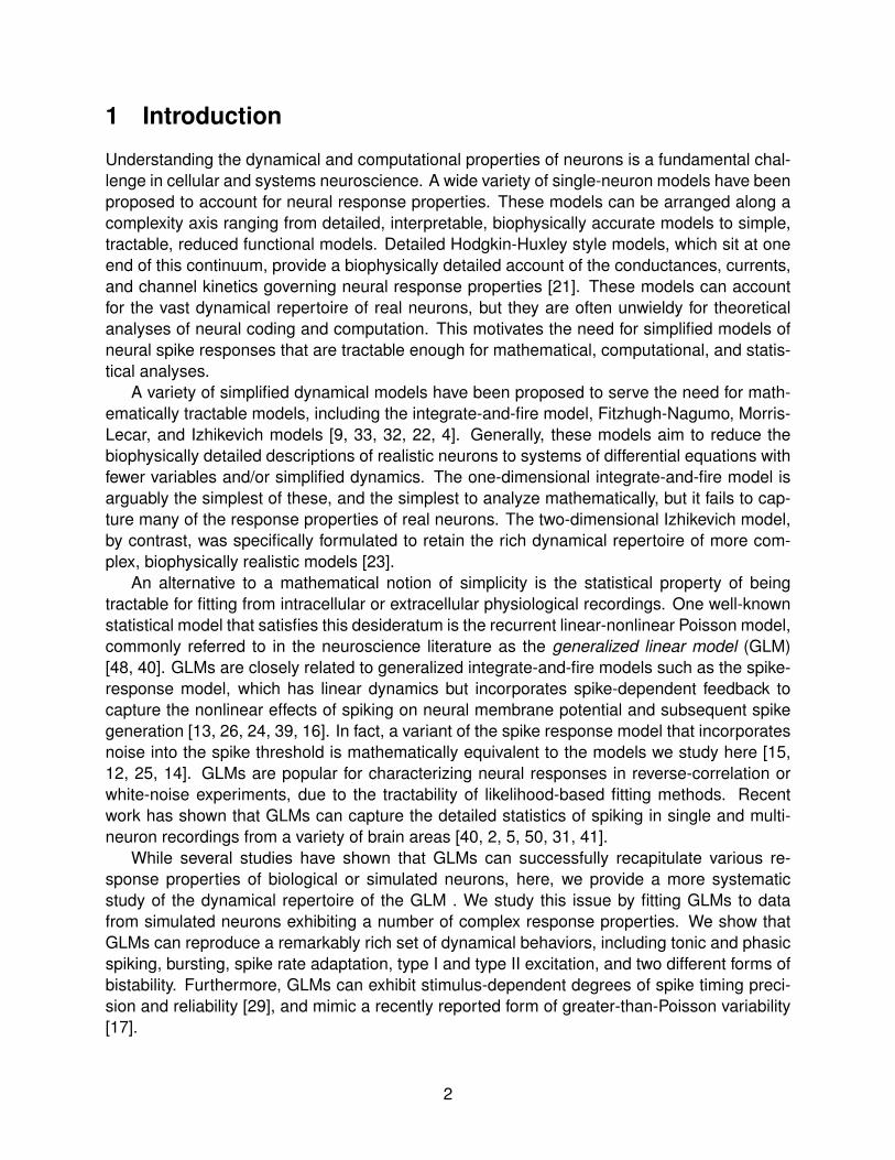
We first examined an Izhikevich neuron tuned to exhibit tonic spiking (Figure 2A-B; see Table1 for parameters). When presented with a step input current, the Izhikevich neuron respondswith a few high-frequency spikes and then settles into a regular firing pattern that persists forthe duration of the step (Figure 2B). This response pattern resembles that of a deterministicHodgkin-Huxley or integrate-and-fire neuron, albeit with an added transient burst of spikes atstimulus onset.

We simulated the Izhikevich neuron’s response to a series of step currents and used theresulting training data to perform maximum-likelihood fitting of the GLM parameters {~k,~h, µ}.The estimated stimulus filter ~k is biphasic (Figure 2C), resulting in a large transient responseto stimulus onset, and has a positive integral, ensuring a sustained positive response to a

Izhikevich neuron response

A!

E

F

G

inpu

tm

Vfil

ter o

utpu

ts

resp

onse

s

GLM repeats

conditional!intensity

time (ms)

stimulusC!

time (ms)

(sp/

s)

Izhikevich

= -35

fitted GLM parameters

B

D

stimulus filter

post-spike filter

output

output

0 200 400 600

12

0

10

10

106

-2000

0

2000

-80-3020

05

10

-100 -50 0

-0.50

0.51

1.5

0 50 100-1000

-750

-500

-250

0

Figure 2: Tonic spiking behavior. A: A step current stimulus. B: Voltage response of thesimulated Izhikevich neuron. C: The fitted GLM stimulus filter ~k has a biphasic shape thatgives the model a vigorous response to stimulus onset and a net positive response to a sus-tained input. D: The fitted GLM post-spike filter ~h has a negative lobe that imposes strongrefractoriness on a timescale of ≈50 ms. E: Stimulus (blue) and post-spike (red) filter outputsduring simulated response of the fitted GLM to the stimulus shown above on a single trial. F:The summed filter outputs are passed through an exponential nonlinearity to determine theconditional intensity λ(t), shown here for a single trial. G: Spike train of the Izhikevich neuron(black) and simulated repeats of the GLM (gray). GLM spike responses are slightly different oneach trial, due to the stochasticity of spike generation, but reproduce Izhikevich model spiketimes with high precision.

5

current step (Figure 2E, blue trace). The estimated post-spike filter ~h (Figure 2D), by contrast,has a large negative lobe that provides recurrent inhibition after every spike, enforcing a strongrelative refractory period. The stimulus filter and post-spike filter output (shown together fora single trial in Figure 2E) are summed together and exponentiated to obtain the conditionalintensity λ(t) (Figure 2F), also known as the instantaneous spike rate.

For this stimulus, the intensity rises very quickly once ~h decays, which occurs approxi-mately 50 ms after the previous spike. Note that the output of the stimulus filter is identicalon each trial, whereas the the output of the post-spike filter varies from trial to trial becauseof variability in the exact timing of spikes. However, because the rising phase of the condi-tional intensity is so rapid, spiking is virtually certain within a small time window sitting at afixed latency after the previous spike time. The combination of strong excitatory drive from thestimulus filter and strong suppressive drive from the post-spike filter produces precisely timedspikes across trials, allowing the GLM to closely match the deterministic firing pattern of theIzhikevich neuron (Figure 2G).

3.2 Bursting

We next examined multi-spike bursting, a more complex temporal response pattern that re-quires dependencies beyond the most recent interspike interval. Once again, we simulatedresponses from an Izhikevich neuron tuned to exhibit tonic bursting (Figure 3A-B) and usedthe resulting data to fit GLM parameters (Figure 3C-D). The estimated stimulus filter ~k is bipha-sic with a larger positive than negative lobe, which drives rapid spiking at stimulus onset andgenerates sustained drive during an elevated stimulus (Figure 3E, blue trace). The post-spikefilter ~h has an immediate negative component that creates a relative refractory period aftereach spike, and an even more negative mode after a latency of ≈40 ms; the accumulationof these negative components over multiple spikes gives rise to a sustained suppression ofactivity between bursts.

The GLM captures the bursting behavior of the Izhikevich neuron with high precision, in-cluding the fact that the first burst after stimulus onset contains a different pattern of spikesthan subsequent bursts. This difference arises from precise interactions between the stimulusand post-spike filter outputs. During the first burst, fast spiking arises from an interplay be-tween monotonically increasing stimulus filter output (Figure 3E, blue) and tonic decrementsinduced by the post-spike filter after each spike (Figure 3E, red). After each spike, the post-spike filter reduces the conditional intensity by a fixed decrement, but this decrement is soonoverwhelmed by the rising wave of input from the stimulus filter, which creates a rapid rise andfall of the conditional intensity time-locked to each Izhikevich neuron spike time. The patterncontinues until accumulated contributions from the delayed negative lobes of post-spike filteroverwhelm those from the stimulus filter and the burst terminates. Subsequent bursts are gov-erned by a somewhat different interplay between stimulus and post-spike filter outputs: burstssit on a rising phase of the conditional intensity due to the removal of suppression from theprevious burst. This rise is more gradual than the drive induced by stimulus onset, and resultsin bursts with longer inter-spike intervals and fewer spikes per burst, but the resulting spikepattern is nonetheless captured with high precision and reliability from trial to trial.

6

3

Izhikevich neuron response

A!

E

F

G

inpu

tm

Vfil

ter o

utpu

ts

resp

onse

s

GLM repeats

conditional!intensity

time (ms)

stimulus

C!

time (ms)

(sp/

s)

Izhikevich

= -121

fitted GLM parameters

B

D

stimulus filter

post-spike filter

output

output

0 50-200

-150

-100

-50

0

-100 -50 0

-0.10

0.10.20.30.4

0

10

-80-3020

-1000-500

0500

106

01010

0 100 200 300 400100

Figure 3: Bursting behavior. A: Step current stimulus. B: Voltage response of Izhikevich neu-ron. C: Fitted GLM stimulus filter. D: Fitted GLM post-spike filter, which creates refractorinesson short timescales (within each burst) due to instantaneous depolarization following a spike.The large negative lobe ≈25-50 ms after a spike terminates bursting and strongly suppressesfiring between bursts. E: Stimulus (blue) and post-spike (red) filter outputs for simulated re-sponse of the GLM to step current shown above on a single trial. F: Output of the nonlinearity(conditional intensity) λ(t) on a single trial. G: Spike train of Izhikevich neuron (black) andsimulated repeats of the fitted GLM (gray).

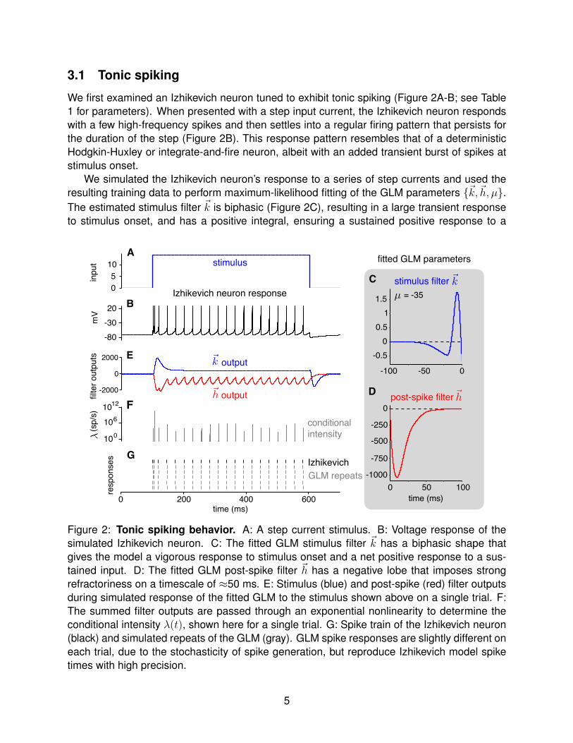
3.3 Bistability

Bistability refers to the phenomenon in which there are multiple stable response modes fora single input condition. A common form of bistability observed in real neurons is the abilityto inhabit either a tonically active state or a silent state for a given level of current injection.The Izhikevich model can exhibit this form of bistability, wherein a brief positive current pulseis sufficient to kick it between states: the neuron can inhabit a silent state in the absenceof stimulation, but a brief positive current pulse kicks it into a tonically active state, and anappropriately-timed positive pulse kicks it back to the silent state (Figure 4A-B).

We fit a GLM to spike trains simulated from such a bistable Izhikevich neuron and foundthat the fitted GLM can capture bistable behavior of the original model with high accuracy(Figure 4C-G). When stimulated during the silent state, the GLM emits a spike due to thepositive output of the stimulus filter (Figure 4E, blue), and tonic firing ensues due to a positivelobe in the post-spike filter that causes self-excitation at a fixed latency of approximately 10 msafter the previous spike (Figure 4E). The GLM returns from the active state to the silent statewhen a positive stimulus pulse synchronizes negative lobes of the stimulus and post-spike

7

filters. Only the combination of these two negative drives is strong enough to shut off spiking;without the negative drive created by previous spikes (appearing in the post-spike filter at alatency of 15 ms after a spike), suppression from the negative lobe of the stimulus filter isnot strong enough to prevent spiking. As with the tonic spiking neuron discussed above, theinteraction between the stimulus and post-spike filters generates rapid rises in the conditionalintensity (Figure 4F), leading to precisely timed spikes that mimic those of the deterministicIzhikevich neuron (Figure 4G).

This Izhikevich neuron (with the same parameters) can also exhibit a second form of bista-bility, in which the return to the silent state from the active state is induced by a negativeinstead of a positive current pulse. We performed a similar fitting exercise and found that theGLM is also able to reproduce this behavior. Firing is initiated and maintained by a similarmechanism as the first form of bistability, but firing offset occurs due to the fact that a negativestimulus pulse creates immediate negative output from the stimulus filter, which suppressesfiring during the time when a spike would have occurred due to spike-history filter input. Tonicfiring is extinguished more rapidly in this second form of bistability than the first (see Figure 6

Izhikevich neuron response

A!

E

F

G

inpu

tm

Vfil

ter o

utpu

ts

resp

onse

s

GLM repeats

conditional!intensity

time (ms)

stimulus

C!

time (ms)

(sp/

s)

Izhikevich

= -204

fitted GLM parameters

B

D

stimulus filter

post-spike filter

output

output

0

6

0

10

10

103

-60-50-40

-80-3020

-400-200

0

50 100

-100 -50 0-0.02

0

0.02

0 10 20

-400

-200

0

Figure 4: Bistable responses. A: Stimulus consisting of two brief positive current pulses.B: Voltage response of Izhikevich neuron, which exhibits bistability. The first pulse initiates atonic spiking mode and the second pulse (precisely timed to the phase of the spike response)terminates it, returning to a quiescent mode. C: Fitted GLM stimulus filter, which provides abiphasic impulse response. D: Fitted post-spike filter, which imposes a refractory period of≈4 ms and gives increased probability of firing ≈5-10 ms after each spike. E: GLM stimulus(blue) and post-spike (red) filter outputs on a single trial. F: Output of the nonlinearity gives theconditional intensity for a single trial. G: Spike train of Izhikevich neuron (black) and simulatedrepeats of the fitted GLM (gray).

8

below).

3.4 Type I and type II firing

Neurons have been classified as exhibiting either type I or type II dynamics based on theshape of their firing rate vs. intensity (F-I) curve. Type I neurons can fire at arbitrarily lowrates for low levels of injected current, whereas type II neurons have discontinuous F-I curvesthat arise from an abrupt transition from silence to a finite non-zero firing rate as the level ofinjected current increases [20]. We simulated Izhikevich neurons that exhibit each of theseresponse types using published parameters. Inputs consisted of 500 ms current steps ofvarying amplitude. The resulting F-I curves for the Izhikevich type I and type II neurons areshown in black in Figure 5A and Figure 5B, respectively. We fit GLMs using data from eachIzhikevich neuron and found that the fitted GLMs capture the two response types with hightemporal precision. The corresponding F-I curves are shown in gray in Figure 5 and accuratelymimic the behaviors of the Izhikevich neuron. Similar F-I curves have been demonstratedpreviously in [15] and [31].

The only discrepancy between the Izhikevich and GLM neurons occurs for the type II cellat input amplitudes near the Izhikevich neuron’s threshold. On some trials when the inputamplitude falls below this threshold, the GLM jumps into a a tonic firing state for the duration

15 20 25 300

10

20

30

40

input amplitude

firin

g ra

te (H

z)

!!

IzhikevichGLM

0.2 0.4 0.60

10

20

30

40

input amplitude

firin

g ra

te (H

z)

A BType I Type II

Figure 5: Type I and type II firing curves. A: Top: Example responses of a GLM exhibitingtype I firing behavior. The spike rate increases continuously from zero in response to currentsteps of increasing amplitude. Bottom: F-I curve for a type I Izhikevich neuron (black) andcorresponding GLM (gray). For the GLM, responses are plotted for five repetitions of eachinput amplitude. B: Similar plots for type II firing behavior, characterized by a discontinuousjump from zero to a finite spike rate in responses to current steps of increasing amplitude.

9

of the stimulus. Similarly, on some trials when the input amplitude falls above this threshold,the GLM fails to initiate firing. This is unsurprising given the stochastic nature of the GLM.Importantly, the GLM never fires at a low rate, but rather abruptly transitions from no firing tofiring at a baseline level of ≈25 Hz, reflecting type II behavior.

3.5 Additional behaviors

We fit GLMs to every dynamical behavior considered in [23] with the exception of purely sub-threshold behaviors, since GLM fitting uses spike trains and does not consider sub-thresholdresponses. The full suite of behaviors is shown in Figure 6, with responses of the Izhikevichneurons in black and spike responses of the GLM in gray. This list includes tonic and phasicspiking, tonic and phasic bursting, mixed mode firing, spike frequency adaptation, type I andtype II excitability, two different forms of bistability, and several others that depend primarilyon the shape of stimulus filter. Several additional behaviors that can be captured by a GLMare not depicted in Figure 6 as they can be achieved by a trivial manipulation of the stimulusfilter; for example, inhibition-induced bursting can be achieved by simply flipping the sign ofthe stimulus filter for the bursting neuron shown in Figure 6C. Previous work has shown theIzhikevich neuron to be capable of producing 18 distinct spiking behaviors [23], and we foundthat all can also be produced by a GLM.

3.6 Systematic variation of filter amplitudes

We next considered what happens to the behaviors produced by a GLM as some aspect of thefilters is systematically varied. To do so, we created stimulus and post-spike filters composedby linear combinations of two basis filters, and then systematically varied the amplitude of onebasis filter while holding the other fixed. (See Methods for details.) Figure 7 shows the phasespace of qualitative spiking behaviors obtained at different points in this 2D filter space.

When the stimulus filter has a strongly negative component (center panel, bottom), a pos-itive stimulus pulse does not produce enough driving force to cause the neuron to spike at all(quiescent). As the amplitude of this component of the stimulus filter is increased, the neuronreceives stronger and stronger input and is driven first to spike once or twice (phasic spiking),and eventually to emit a burst of spikes (phasic bursting). The stimulus filter largely driveschanges between these behaviors, with the additional detail that a strongly negative post-spike filter component is able to inhibit a burst that would otherwise occur (upper left cornerof “phasic spiking" region). As the stimulus filter component becomes still more positive andthe stimulus filter transitions from being biphasic to more monophasic, it produces a positivedriving force for the duration of the stimulus step, rather than just the onset. This causes theneuron to fire for the duration of the step.

Importantly, the post-spike filter here determines the nature of this sustained firing. Apost-spike filter that is purely negative beginning at short timescales (top, left side) mimics arelative refractory period, inhibiting additional spikes for a short window following each elicitedspike and resulting in tonic spiking. If, on the other hand, the post-spike filter is only weaklynegative at short timescales while being more strongly negative at longer timescales, thiscreates multiple timescales in the neuron’s response (top, right side). At short timescales,

10

A B C D

E F G H

I J K L

M N O P

tonic spiking phasic spiking tonic bursting phasic bursting

mixed mode type I type II

spike latency resonator integrator rebound spike

rebound burst variabilitybistability I bistability II

50 ms

spike frequencyadaptation

threshold

Figure 6: Suite of dynamical behaviors of Izhikevich and GLM neurons. Each panel,top to bottom: stimulus (blue), Izhikevich neuron response (black), GLM responses on fivetrials (gray), stimulus filter (left, blue), and post-spike filter (right, red). Black line in each plotindicates a 50 ms scale bar for the stimulus and spike response. (Differing timescales reflecttimescales used for each behavior in original Izhikevich paper [23]). Stimulus filter and post-spike filter plots all have 100 ms duration.

there is little inhibition from each spike (beyond the absolute refractory period), so additionalspikes may occur. Over longer timescales, inhibition is accumulated over multiple spikes,which eventually shuts off spiking. After a brief window of no spikes, the inhibition is relaxedand spiking commences again until enough inhibition is accumulated to shut spiking off. Thiscycle results in tonic bursting for the duration of the step. In the extreme case where thepost-spike filter is actually biphasic (top, far right), each spike promotes additional spikes onshort timescales, leading to highly regular timing of spikes within bursts (Figure 7C). This set

11

com

pone

nt 2

am

plitu

de

component 1 amplitude

A

B

C

D

A

B D

quiescent

phasic spiking

phasic bursting

tonicbursting

tonicspiking

50 m

s

50 ms

200 ms C

-1 -0.5 0 0.5 1

-1.5

-1

-0.5

0

Figure 7: Changes in a single component of each filter can produce a variety of behav-iors. Center: Amplitudes for a single component of the stimulus filter (ordinate) or post-spikefilter (abscissa) were varied. Responses were simulated for 15 trials of a step stimulus, andthe most common behavior produced is indicated by color. Small panels show example filtersat each extreme of the range tested. A-D: Example responses (gray) to step stimulus (blue)for GLMs with filters indicated by corresponding letter in center panel.

of behaviors could be achieved by simply sweeping over the amplitude of a single basis vectorin each filter. Incorporating shifts to the basis vectors or additional basis vectors would likelybe necessary to achieve more complex behaviors, such as bistability.

Although we have drawn clear borders at the transition between behaviors, these transi-tions in fact occur gradually. Near the border between phasic spiking and phasic bursting, forexample, there will be some trials where a single spike is produced and other trials where aburst is elicited. We have indicated the behavior that is produced most frequently here for sim-plicity. The transition from tonic bursting to tonic spiking also occurs gradually, with the nearperfectly regular bursting breaking down into more irregular firing until no apparent bursts areproduced. If the post-spike filter is made even more negative than the range explored in this fig-ure, the timing of tonic spiking becomes near perfectly regular as well. This is easily explainedby the fact that as the post-spike filter becomes more and more negative, it imposes strongerrefractoriness on the cell, which results in more regular spike timing. As the post-spike filtercomponent amplitude is changed, there is therefore a gradual change from precisely timedbursts, to irregular firing, to precisely timed tonic spiking. In the following section, we furtherexplore questions of spike timing precision in the GLM.

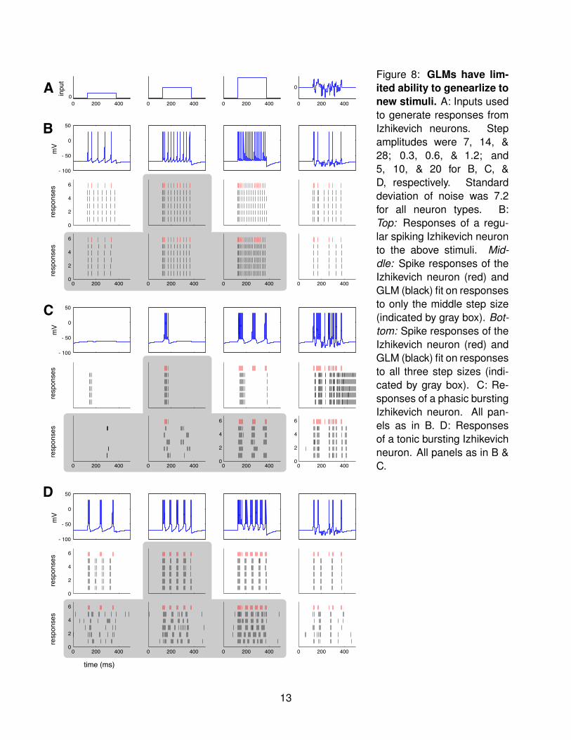
3.7 Generalization to new stimuli

The behaviors shows in Figure 6 were all fit using stimuli that probe only a small range of thepossible behaviors of the neuron. For example, many were probed using only a single stepheight. A natural question that arises is therefore: how well will these fitted GLMs generalize topredict the Izhikevich neuron responses to new stimuli? We examined this question for threecanonical Izhikevich neurons from our study (Figure 8). We first generated responses from a

12

0 200 400 0 200 400 0 200 4000

2

4

6

0 200 4000

2

4

6

- 100

- 50

0

50

A

B

C

D

- 100

- 50

0

50

0

2

4

6

0 200 4000

2

4

6

0 200 400 0 200 400 0 200 400

00

200 400 0 200 400 0 200 400 0

0

200 400

time (ms)

mV

resp

onse

sre

spon

ses

mV

resp

onse

sre

spon

ses

mV

resp

onse

sre

spon

ses

inpu

t

- 100

- 50

0

50

0

2

4

6

0 200 4000

2

4

6

0 200 400 0 200 400 0 200 400

Figure 8: GLMs have lim-ited ability to genearlize tonew stimuli. A: Inputs usedto generate responses fromIzhikevich neurons. Stepamplitudes were 7, 14, &28; 0.3, 0.6, & 1.2; and5, 10, & 20 for B, C, &D, respectively. Standarddeviation of noise was 7.2for all neuron types. B:Top: Responses of a regu-lar spiking Izhikevich neuronto the above stimuli. Mid-dle: Spike responses of theIzhikevich neuron (red) andGLM (black) fit on responsesto only the middle step size(indicated by gray box). Bot-tom: Spike responses of theIzhikevich neuron (red) andGLM (black) fit on responsesto all three step sizes (indi-cated by gray box). C: Re-sponses of a phasic burstingIzhikevich neuron. All pan-els as in B. D: Responsesof a tonic bursting Izhikevichneuron. All panels as in B &C.

13

regular spiking Izhikevich neuron using three step heights and one noise stimulus (Figure 8A;B, top). We then simulated responses to these stimuli using the GLM fit only to the intermediatestep height (Figure 8B, middle). (This is the same fit as Figure 2.) The GLM responses nearlyperfectly capture the Izhikevich responses for the original stimulus, and the GLM maintainsregular firing patterns for the other step heights. However, the GLM’s firing rate is too highfor the small step and too low for the large step. While the GLM accurately captures somefiring events for the noise stimulus, the firing rate is overall too high. We next refit a GLMto responses from all three step heights, using the same set of basis vectors as the originalfit (Figure 8, bottom). The responses to all three step heights are captured nearly perfectly.Additionally, the response to the noise stimulus is much more similar to that of the Izhikevichneuron. Although there is one firing event that occurs at a delay, the regular spiking GLM fit onan enriched stimulus set is better able to generalize to the noise stimulus.

We performed this same test for neurons showing phasic bursting (Figure 8C) and tonicbursting (Figure 8D). (Note that although some responses of the phasic bursting Izhikevichneuron are not actually phasic, we retain the naming convention given to this set of parametersin the original paper.) For phasic bursting, the GLM fit on additional step sizes improves theaccuracy of responses to the smallest and largest steps, while decreasing the accuracy ofresponses for the original step of intermediate size. There is marked improvement in theaccuracy of responses to the noise stimulus, with many firing events being accurately capturedand the GLM no longer exhibiting runaway excitation. For tonic bursting, the refit GLM retainsbursting behavior but fails to even capture responses for the steps on which it was trained.As noted above, when refitting we used the same set of basis vectors as the initial fits for faircomparison. It is possible that by increasing the number of basis vectors used or tuning theirproperties that better fits to all stimuli might be achieved.

Taken together, these results show that while GLMs might retain some characteristic re-sponse features (such as bursting) when probed with new stimuli, they often have limited abilityto generalize beyond stimuli on which they are directly fit.

4 Spiking precision and reliability

A noteworthy feature of the spike trains of the GLM neurons considered above is their highdegree of spike timing precision and reliability across trials. This precision arises from the factthat the conditional intensity (or instantaneous spike rate) rises abruptly at spike times (due tofilter outputs passing through a rapidly accelerating exponential nonlinearity), and decreasesimmediately after each spike due to suppressive effects of the post-spike filter. By contrast, aPoisson GLM without recurrent feedback, more commonly known as a linear-nonlinear Pois-son (LNP) cascade model, cannot produce temporally precise spike responses to a constantstimulus because its output is constrained to be a Poisson process.

Real neurons, however, seem to be capable of both response modes: they emit precisely-timed spikes in some settings and highly variable spike trains in others. A seminal paper byMainen & Sejnowski illustrated this duality by showing that spike responses to a constant DCcurrent exhibit substantial trial-to-trial variability, whereas responses to a rapidly fluctuatinginjected current are precise and repeatable across trials [29]. Deterministic models like theIzhikevich model cannot, of course, mimic this property because their spikes are perfectly

14

0

3

6

9

0 200 400 600 800

5

10

15

time (ms)

constant input fluctuating input

-500

50100

0 200 400 600 800

5

10

15

time (ms)

A B

stim

ulus

am

plitu

detri

al

Figure 9: Stimulus-dependent spike timing reliability. A: Top: Weak step stimulus. Bottom:Spike train responses of tonic-spiking GLM on 15 repeated trials. Although the first spike isprecise and reliable, subsequent spikes have irregular timing from trial to trial. B: Top: Rapidlyfluctuating stimulus. Bottom: Spike response of same GLM neuron on 15 repeated trials,exhibiting a high degree of precision and reliability. (Compare to Figure 1 of [29].)

reproducible for any stimulus. (A stochastic version of the Izhikevich model with an appropriatelevel of injected noise could likely overcome this shortcoming, however. See [44] for a similarcase in a Hodgkin-Huxley neuron.) Here we show that the GLM naturally reproduces thesame form of stimulus-dependent changes in precision and reliability observed in real neurons.Figure 9 shows that a single GLM (with parameters identical to those fit to the tonic-spikingIzhikevich neuron, shown in Figure 2) produces irregular spiking in response to a constantstimulus with low-to-intermediate amplitude, and precisely-timed, reliable spikes in responseto a stimulus with large, rapid fluctuations.

5 GLMs can produce super-Poisson variability

We have shown that GLM neurons can reproduce the high degree of spike timing precisionfound in real neurons stimulated with injected currents. However, a variety of studies havereported that neurons exhibit overdispersed responses, or greater-than-Poisson spike countvariability in response to repeated presentations of a sensory stimulus [47, 46, 45, 17]. Aprominent recent study from Goris, Movshon, & Simoncelli showed that the degree of overdis-persion grows with mean spike count, so that the Fano factor (variance-to-mean ratio) is anincreasing function of spike rate [17]. They proposed a doubly stochastic model to account forthis phenomenon, in which the rate of a Poisson process is modulated by a slowly fluctuatingstochastic gain variable g. For each trial, g is drawn from a gamma distribution with mean 1and variance σ2

g . (See Methods for details.)We sought to determine if a GLM with spike-history dependence can also account for

the mean-dependent overdispersion found in neural responses. To test this possibility, wesimulated spike trains from the doubly stochastic model of Goris et al for three different settings

15

of the over-dispersion factor σ2g with the same mean spike rate (100 spikes/s), and fit a GLM

to the spike trains associated with each value of σ2g . We then simulated responses from each

GLM to 500 ms pulses at a number of different input intensities, with each point in Figure 10corresponding to a different intensity.

We found that the GLM can indeed match the qualitative behavior of the Goris et al model,giving approximately Poisson responses at low spike rates and increasingly overdispersed re-sponses at higher rates (Figure 10C). To match the data from larger values of overdispersionfactor σ2

g (darker curves in Figure 10C), the GLM relies on increasing amounts of self-excitationfrom the post-spike filter, but exhibits no changes in stimulus filter (Figure 10A-B). The filtershere do not include an absolute refractory period, as the original model does not incorporateone. However, similar results can be achieved when a refractory period is enforced in the train-ing data. This will result in post-spike filters with strongly negative lobes on short timescales,which impose refractoriness, but otherwise similar filters to those in Figure 10. Unlike modelswith purely suppressive spike history effects, which capture effects due to refractoriness andreduce variability in firing (e.g., [3, 49]), here we show that allowing spike history effects to beexcitatory can result in increased variability. While the former might be suitable for early sen-sory areas, such as the retina, the latter better captures the super-Poisson variability observedin higher visual areas.

Intuitively, the GLM generates overdispersed spike counts because of dependencies thespike-history filter induces between early and late spikes during a trial: if the GLM neurongenerates a larger-than-average number of spikes early in a trial, the positive post-spike filterproduces a higher conditional intensity (and hence more spiking) later in the trial; conversely, ifa neuron emits fewer-than-average spikes early in a trial, the conditional intensity will be lowerlater in the trial (yielding less spiking). The Goris et al model can be seen to capture similardependencies between early and late spikes via the stochastic gain variable g, which is con-stant during a trial but independent across trials. Thus, it is reasonable to view g in the Goris et

0 20 40 60 80 1000

100

200

300

400

spike count mean

Poisson spikingspik

e co

unt v

aria

nce

-50 -25 0

0

0.1

0.2

0 200 400

0

0.02

time (ms)

= -0.84 = -1.11

= -0.86

time (ms)

Astimulus filters spike-history filters

B C

Figure 10: GLMs can produce super-Poisson variability. A: Stimulus filters for GLMs trainedon three different levels of variability: high (dark blue), medium (medium), and low (light) super-Poisson variability. Spike count mean was identical in the three cases: 100 spikes/s. B: Post-spike filters for high (dark red), medium (medium), and low (light) super-Poisson variability. C:Spike count variance versus mean for three levels of variability. This relationship is strikinglysimilar to that observed in many cortical neurons.

16

al model as a proxy for the accumulated self-excitation from spike-history filter outputs undera GLM. We note, however, that attempts to drive the GLM to higher levels of overdispersion(e.g., Fano factors significantly > 3) often resulted in runaway self-excitation, indicating thatGLMs may require additional mechanisms to maintain stability in order to produce highly over-dispersed responses through recurrent excitation alone [11, 19]. An alternative mechanismfor generating over-dispersed responses with GLMs is through the addition of latent stochasticinputs [42], an avenue we have not explored here.

6 Discussion

We have shown that recurrent Poisson GLMs can capture an extensive set of behaviors exhib-ited by biological neurons, including tonic and phasic spiking, bursting, spike frequency adap-tation, type I and type II behavior, and bistability. GLMs can also reproduce widely varyinglevels of response stochasticity, ranging from precisely timed spikes with negligible trial-to-trialvariability, to substantially super-Poisson spike count variability. We have also shown that, likereal neurons, GLMs can exhibit irregular firing in response to a constant stimulus, but preciseand repeatable firing patterns in response to a temporally varying stimulus. Thus, generalizedlinear models are able to capture a rich array of spiking behaviors like many dynamical models,while remaining tractable to fit to neural data.

6.1 Relationship to previous work

As mentioned above, GLMs have strong connections to a number of other models. It is partic-ularly worth noting the connection between GLMs and generalized integrate-and-fire models,such as the spike response model (SRM) extensively studied by Gerstner and colleagues[15, 13]. These models draw on much earlier work which incorporated a variable thresholdthat depends on spiking history [51, 10]. The SRM includes a membrane filter (analogous tothe stimulus filter here) and both a spike afterpotential and moving threshold (which can becombined and are analogous to the spike history filter here). In its simplest formulation, theSRM is a deterministic model. Although the threshold for spiking can shift as a function ofspike history, a spike will occur precisely at each threshold crossing.

Extensions of the model have incorporated so-called “escape noise," where spiking nolonger occurs deterministically at threshold crossings, but rather the probability of spiking de-pends on the distance of the membrane voltage to threshold [15, 25]. This variant of the SRMis in fact a GLM, and it is therefore worthwhile to consider how previous work investigatingthe SRM with escape noise relates to our results here. Early work demonstrated that such amodel was capable of producing responses with high temporal precision, including both tonicspiking as well as tonic bursting [15], though demonstrating the range of behaviors that couldbe produced by the SRM was not the focus of this study. Additional work demonstrated that themodel could produce highly repeatable spike trains to a noisy stimulus (similar to Figure 9B,though no comparison of irregular firing in response to a constant stimulus was shown) [25].Other studies have shown that the SRM can capture the detailed statistics of neural responses[31, 41]. Further, many of these studies show that the spike responses model can be usedto capture not only the relationship between an external stimulus and a neuron’s response,

17

but also to faithfully capture the relationship between intracellularly recorded neural responsesand injected current [25, 41].

6.2 Limitations

Despite their many advantages, GLMs have several limitations that bear further discussion.First, GLMs often do not generalize well across stimulus distributions; models fit with a partic-ular set of stimuli often do not accurately predict responses to stimuli with markedly differentstatistics (e.g., stimuli with large changes in mean or variance, or white noise vs. naturalisticstimuli) [18].

Secondly, GLMs often lack clear interpretability in terms of underlying mechanisms. Thisstands in contrast to dynamical models designed to capture specific biophysical variables andprocesses. In the two-dimensional Izhikevich model, for example, one variable (v) representsthe neuron’s membrane potential, and the other variable (u) can be understood as a membranerecovery variable, which reflects K+ channel activation and Na+ channel inactivation. Despitethe fact the GLM filters do not represent specific biophysical variables, in some cases they canstill provide insight into underlying biological processes. For example, recent work provides aninterpretation of the GLM as a synaptic conductance based model with linear sub-thresholddynamics [27]. Work on the SRM has shown that by dividing the effects of spike history into adynamic threshold and a spike afterpotential, one can in fact measure their separate contribu-tions with intracellular recordings of a neuron’s subthreshold voltage; the spike afterpotentialcan be observed directly in this voltage trace, while the effects on thereshold can be estimatedindirectly by noting the absence of firing [31, 41, 14].

A third known limitation of GLMs is that they lack the flexibility to capture some nonlinearresponse properties of real spike trains. For example, as point neuron models, GLMs do notreflect the fact that neurons often receive spatially segregated inputs on the dendritic tree, andthese inputs can be processed separately and combined nonlinearly [28]. Some extensions ofthe GLM that incorporate nonlinear inputs and multiple subunits [8, 43, 36, 7, 30, 1, 52] maybegin to address this issue, but certainly fall short of capturing the full complexity of dendriticprocessing. For the range of dynamical behaviors considered here, however, we did not findthese extensions to be necessary.

For all results shown, we used a GLM with an exponential nonlinearity. To test the depen-dence of our results on the form of the nonlinearity, we also fit GLMs to several of the behaviorswith a “soft-rectifying” nonlinearity given by f(x) = log (1 + exp (x)). This function grows onlylinearly for large input values, but still has an exponential decay on its left tail and remainsin the family of nonlinearities (convex and log-concave) for which the GLM log-likelihood isprovably concave [34]. For the behaviors tested (tonic spiking, tonic bursting, phasic spiking,and phasic bursting), our results were similar to those with an exponential nonlinearity, thoughgenerally not as temporally precise. This increased precision is likely due to the fact that anexponential nonlinearity rises more steeply than a linear-rectifying function, causing the condi-tional intensity to accelerate more rapidly from a low-probability to a high-probability of spikingregime. Past studies have found that responses of both retinal ganglion cells and neocorticalpyramidal neurons are well described by a GLM with exponential nonlinearity [40, 25].

It is worth noting that for many of the dynamic behaviors studied here, the GLM parameters

18

were not strongly constrained by the training data. (See "Sensitivity to changes in parametervalues" in Appendix.) Slight changes in the model parameters did not produce noticeablechanges in response, at least for the stereotyped range of input currents and output spikepatterns considered. The filter parameters were therefore only weakly identifiable, which cor-responds to a likelihood function with a very gradual falloff along certain directions in parameterspace. This uncertainty potentially complicates interpretation of the filters in terms of functionsperformed by the underlying biophysical mechanism. Conversely, it reveals that the suite ofbehaviors considered by Izhikevich and others can be achieved by a range of different GLMs,and that a richer set of input-output patterns is needed to identify a unique set of GLM param-eters.

Conclusion

The GLM has the ability to mimic a wide range of biophysically realistic behaviors exhibited byreal neurons. Although it is clear there are some forms of nonlinear behavior it cannot produce,such as frequency-doubled responses of cat Y cells or V1 complex cells to a contrast-reversinggrating, our work provides an existence proof for its ability to exhibit an important range of re-sponse types considered previously only in biophysics and applied math modeling literature.Moreover, by considering response stochasticity as another dimension along which real neu-rons vary, we have shown that that the GLM can generate response characteristics rangingfrom quasi-deterministic to greater-than-Poisson variability. The GLM therefore provides aflexible yet powerful tool for studying the dynamics of real neurons and the computations theycarry out.

Appendix

MATLAB code used to generate example responses from Izhikevich neurons and to fit GLMsto these responses is available in a Github repository (https://github.com/aiweber/GLM_and_Izhikevich).

Izhikevich model simulations

To generate training data for fitting the GLM, we simulated responses from an Izhikevich model[22] with parameters set to published values given for each behavior in [23] (Table 1; parametervalues can be found at http://www.izhikevich.org/publications/izhikevich.m). For each behavior,we generated approximately 20 seconds of training data using the forward Euler method withfixed time step size (dt) given in Table 1. It should be noted that in some cases, published pa-rameter values did not produce the desired qualitative behavior. In these cases, we tuned thesimulation parameters to achieve the desired behavior. Parameters marked with an asterisk inTable 1 indicate those that differ from published values for the corresponding behavior in [23].Additionally, some behaviors of the Izhikevich neuron are not robust to small changes in stim-ulus timing, stimulus amplitude, or time step of integration. In particular, we found bistability to

19

be highly dependent on the precise stimulus timing (onset and duration), stimulus amplitude,and integration window. We tuned these values by hand to produce the desired behavior.

GLM fitting and simulations

A generalized linear model for a single neuron attributes features of a spike train to both stimu-lus dependence and spike history. Stimulus dependence is captured by a stimulus filter k, andspike-history dependence is captured by a post-spike filter h. k and h are represented with araised cosine basis to reduce to the dimensionality necessary to fit and ensure smoothness ofthe filters. Basis vectors are of the form:

bj(t) =1

2cos(a log[t+ c]− φj) +

1

2(6)

for t such that a log(t+ c) ∈ [φj −π, φj +π] and 0 elsewhere. The parameter c determines theextent to which peaks of the basis vectors are linearly spaced, with larger values of c resultingin more linear spacing. We typically used 6 such basis vectors to fit a 100 ms stimulus filterk and 8 basis vectors to fit a 150 ms post-spike filter h, for a total of 15 parameters (including

neuron type a b c d I dt (ms)

tonic spiking 0.02 0.2 -65 6 14 0.1

phasic spiking 0.02 0.25 -65 6 0.5 0.1

tonic bursting 0.02 0.2 -50 2 10* 0.1

phasic bursting 0.02 0.25 -55 0.05 0.6 0.1

mixed mode 0.02 0.2 -55 4 10 0.1

spike frequency adaptation 0.01 0.2 -65 5* 20* 0.1

type I 0.02 -0.1 -55 6 25 1

type II 0.2 0.26 -65 0 0.5 1

spike latency 0.02 0.2 -65 6 3.49* 0.1

resonator 0.1* 0.26 -60 -1 0.3 0.5

integrator 0.02 -0.1 -66* 6 27.4 0.5

rebound spike 0.03 0.25 -60 4 -5 0.1

rebound burst 0.03 0.25 -52 0 -5 0.1

threshold variability 0.03 0.25 -60 4 2.3 1

bistability I 1 1.5 -60 0 30* 0.05

bistability II 1 1.5 -60 0 40 0.05

Table 1: Parameters of the Izhikevich neuron for dynamic behaviors shown in Figures 2-6, 8-9, & 11. Parameters marked with * indicate parameters that differ from those used in [23].Additionally, only a single form of bistability (bistability I) was presented in [23].

20

one for µ that determines baseline firing rate). In some cases, as few as 7 or as many as26 parameters were used to fit an individual Izhikevich neuron’s behavior. In general, thefewest number of basis vectors required to reproduce a given behavior were used, though itis likely that by altering specific features of the basis vectors (e.g., their spacing), even fewerparameters would suffice.

We fit the model parameters (weights on the basis functions for k, weights on the basisfunctions of h, and µ) by maximizing the log-likelihood:

L(θ) =∑

t=spike

log λ(t)−∆∑t

λ(t) (7)

where ∆ is the time resolution of y(t). We used MATLAB’s fminunc function, part of theMATLAB optimization toolbox, to find the global maximum of the likelihood function.

We simulated the GLM response in time bins of the same size as the corresponding Izhike-vich neuron and computed the single-bin probability of a spike as

P (y(t) ≥ 1|λ(t)) = 1− P (y(t) = 0|λ(t)) = 1− exp(∆λ(t)), (8)

where ∆ is the time bin size, so that the probability of 0 or 1 spikes in a bin sums to 1 (resultingin a Bernoulli approximation to the Poisson process), disallowing spike counts greater than 1in a single bin.

Systematic variation of filter amplitudes

In order to more carefully examine the transitions between different behaviors as the stimulusand post-spike filter change, we systematically varied the amplitude of individual filter compo-nents and observed the behavior produced. Each filter was parameterized with 2 components.The amplitude of one was fixed while the amplitude of the other was varied. For the stimulusfilter, the amplitude of the second component was varied (-1.5 to +0.25). This allowed us totransition from monophasic to biphasic filters. The amplitude of the first component was set tobe positive (+1), creating an “ON" filter appropriate for a positive step stimulus. For the post-spike filter, the amplitude of the first component was varied (-1 to +1). The amplitude of thesecond component was set to be negative (-3), ensuring that spiking would be suppressed onlonger timescales. For the post-spike filter we also imposed an absolute refractory period of 5ms. Finally, we included a negative baseline drive (µ = -1) to suppress spontaneous spikingso that the baseline firing rate was zero.

We simulated responses to 25 identical step stimuli for each set of filters and then classi-fied the behaviors as quiescent, phasic spiking, phasic bursting, tonic spiking, or tonic bursting.The most commonly observed behavior over the 25 repetitions is depicted in Figure 7. Re-sponses were classified in the following way. If no spikes were elicited in the first 200 ms ofstimulus presentation and fewer than 5 spikes were elicited during the final 10 seconds of stim-ulus presentation, the behavior was classified as quiescent. If at least one spike was elicitedin the first 200 ms following stimulus onset and fewer than 5 spikes were elicited during thefinal 10 seconds of stimulus presentation, the behavior was classified as phasic. Phasic firingpatterns were further classified into phasic spiking if only 1 or 2 spikes were elicited in thefirst 200 ms, and phasic bursting if 3 or more spikes were elicited in the first 200 ms. The

21

remaining responses were classified as either tonic spiking or tonic bursting in the followingmanner. Inter-spike interval distributions were fit with a Gaussian mixture distribution usingMATLAB’s gmdistribution function. We fit both a single Gaussian distribution as well asa mixture of two Gaussians and then compared the Akaike information criterion (AIC) valuesto determine whether the ISI distribution was better fit as a unimodal distribution or a bimodaldistribution, with a lower AIC indicating better fit. If 0.9 · AICunimodal < AICbimodal, the spiketrain was classified as tonic spiking; otherwise, it was classified as tonic bursting. (We addedthe 0.9 factor to create a more stringent standard for what is classified as bursting activity sothat the responses that fall into this category are strongly bimodal distributions that would bereadily identified as bursting. Slightly altering the value of this factor, or eliminating it entirely,gives the same qualitative results, but merely shifts the boundary in Figure 7 between the tonicspiking and tonic bursting regions.)

D

E F

2 4 6 8 10 12 1410

ï 1

100

101

102

eigenvector

0 25 50 75 100

- 0.2

0

0.2

0.4

0.6

most constrained

0 25 50 75 100- 300

- 200

- 100

0

100

time (ms)

0 25 50 75 100

least constrained

0 25 50 75 100

time (ms)

tonic bursting

z-

sco

red

co

effi

cie

nt

filte

r

am

plit

ude

filte

r

am

plit

ude

A

B

2 4 6 8 10 12 1410

ï 8

10ï 4

100

eigenvector

0 25 50 75 100- 1

0

1

2

most constrained

0 50 100 150

- 1000

- 500

0

time (ms)

0 25 50 75 100

least constrained

0 50 100 150

time (ms)

regular spiking

C

filte

r

am

plit

ude

z-

sco

red

co

effi

cie

nt

filte

r

am

plit

ude

Figure 11: Sensitivity to changes in parameter values for a regular spiking (left) and tonicbursting (right) GLM. A: Fit coefficient of each eigenvector of Hessian matrix of likelihood,normalized by corresponding eigenvalue. Eigenvectors are in order of decreasing eigenvalues(not necessarily decreasing z-scored eigenvalues). B: Stimulus filter (top, blue) and spikehistory filter (bottom, red), along with two most constrained eigenvectors. These correspondto the largest (dark gray) and second largest (light gray) eigenvalues. Eigenvectors are scaledto size comparable with filters. C: Same as B, for least constrained eigenvectors. D-F: Sameas A-D for tonic bursting neuron.

22

Sensitivity to changes in parameter values

We wished to investigate how well constrained different features of our fit GLMs were. Todo so, we calculated the eigendecomposition of the Hessian matrix of the likelihood function:H = QΛQ−1. The Hessian matrix provides a local quadratic approximation to the likelihoodfunction, with eigenvectors qi pointing along the principal axes and length of these axes propor-tional to 1√

λi. Thus, larger magnitude eigenvalues indicate greater curvature (i.e., shorter axes)

and better constrained directions, while smaller magnitude eigenvalues indicate lower curva-ture and more poorly constrained directions. Results of this analysis are shown in Figure 11for both a regular spiking neuron (left) and tonic bursting neuron (right). For both neurons, theleast constrained directions correspond to eigenvectors similar in shape to the best-fit filters orthe absolute refractory period. As such, perturbations in these directions do not result in largechanges in the behavior. Perturbations along eigenvectors corresponding to the most con-strained directions, on the other hand, would result in significant changes to the filter shape.The difference in scale between Panel A and Panel D indicates that overall, parameters for thetonic bursting neuron are more constrained than those for the regular spiking neuron.

Doubly stochastic model with super-Poisson variability

In Figure 10, we used a negative binomial model to generate spike trains with greater-than-Poisson variability [38, 17]. The negative binomial distribution can be conceived as a doubly-stochastic model in which the rate of a Poisson process is modulated by an iid gamma randomvariable on each trial. Following [17], we modeled responses with a stochastic gain variable gwith mean 1 and variance σ2

g that obeys a gamma distribution:

P (g|r, s) =1

srΓ(r)gr−1 exp

(−gs

), (9)

where s = σ2g denotes the scale parameter, r = 1/σ2

g is the shape parameter, and Γ(·)represents the gamma function.

The spike count conditioned on g and a stimulus S for each trial then obeys a Poissondistribution:

P (y|g, S) =(∆gf(S))y

y!exp (−∆gf(S)) , (10)

where ∆ is the time bin size, g is the gain, and f(S) is the tuning curve that specifies themean response to stimulus S. In the limit σ2

g = 0, the gain g is deterministically equal to 1and the spike count is Poisson with mean and variance equal to ∆f(S). For responses withσ2g > 0, however, responses are overdispersed relative to the Poisson distribution and have

mean ∆f(S) and variance ∆f(S)(1 + σ2g∆f(S)).

For the results shown in Figure 10, we simulated data from the negative binomial dis-tribution with a single mean rate f(S) (100 spikes/s) at three different gain variances σ2

g ∈{.0125, 0.02, 0.05}. Spike counts were drawn iid across trials, with spike times distributed uni-formly within each trial to generate spike trains suitable for GLM fitting. We used these spiketrains to fit a GLM to the data associated with each value of σ2

g , with an assumed constantinput current for each trial.

23

Acknowledgments

We would like to thank Adrienne Fairhall, Sara Solla, and James Fitzgerald for helpful com-ments and discussions.

References

[1] Ahrens, M. B., Linden, J. F., and Sahani, M. (2008). Nonlinearities and contextual influ-ences in auditory cortical responses modeled with multilinear spectrotemporal methods. JNeurosci, 28(8):1929–1942.

[2] Babadi, B., Casti, A., Xiao, Y., Kaplan, E., and Paninski, L. (2010). A generalized linearmodel of the impact of direct and indirect inputs to the lateral geniculate nucleus. Journal ofVision, 10(10):22.

[3] Berry, M. and Meister, M. (1998). Refractoriness and neural precision. Journal of Neuro-science, 18:2200–2211.

[4] Brette, R. and Gerstner, W. (2005). Adaptive exponential integrate-and-fire model as aneffective description of neuronal activity. Journal of neurophysiology, 94(5):3637–3642.

[5] Calabrese, A., Schumacher, J. W., Schneider, D. M., Paninski, L., and Woolley, S. M. N.(2011). A generalized linear model for estimating spectrotemporal receptive fields fromresponses to natural sounds. PLoS One, 6(1):e16104.

[6] Cox, D. and Isham, V. (1980). Point Processes. Chapman & Hall/CRC Monographs onStatistics & Applied Probability. Taylor & Francis.

[7] Cui, Y., Liu, L. D., Khawaja, F. A., Pack, C. C., and Butts, D. A. (2013). Diverse sup-pressive influences in area mt and selectivity to complex motion features. The Journal ofNeuroscience, 33(42):16715–16728.

[8] Fitzgerald, J. D., Rowekamp, R. J., Sincich, L. C., and Sharpee, T. O. (2011). Second orderdimensionality reduction using minimum and maximum mutual information models. PLoSComput Biol, 7(10):e1002249.

[9] FitzHugh, R. (1961). Impulses and physiological states in theoretical models of nervemembrane. Biophysical journal, 1(6):445.

[10] Geisler, C. D. and Goldberg, J. M. (1966). A Stochastic Model of the Repetitive Activity ofNeurons. Biophysical Journal, 6(1):53–69.

[11] Gerhard, F., Deger, M., and Truccolo, W. (2017). On the stability and dynamics of stochas-tic spiking neuron models: Nonlinear hawkes process and point process glms. PLoS com-putational biology, 13(2):e1005390.

[12] Gerstner, W. (1995). Time structure of the activity in neural network models. PhysicalReview E, 51(1):738–758.

24

[13] Gerstner, W. (2001). A framework for spiking neuron models: The spike response model.In Moss, F. and Gielen, S., editors, The Handbook of Biological Physics, volume 4, pages469–516.

[14] Gerstner, W., Kistler, W. M., Naud, R., and Paninski, L. (2014). Neuronal Dynamics:From Single Neurons to Networks and Models of Cognition. Cambridge University Press,New York, NY, USA.

[15] Gerstner, W. and van Hemmen, J. (1992). Associative memory in a network of ‘spiking’neurons. Network: Computation in Neural Systems, 3(2):139–164.

[16] Gerstner, W., van Hemmen, J. L., and Cowan, J. D. (1996). What matters in neuronallocking? Neural computation, 8:1653–1676.

[17] Goris, R. L. T., Movshon, J. A., and Simoncelli, E. P. (2014). Partitioning neuronal vari-ability. Nat Neurosci, 17(6):858–865.

[18] Heitman, A., Greschner, M., Field, G., Li, P., Ahn, D., Sher, A., Litke, A., and Chichilnisky,E. (2014). Representation and reconstruction of natural scenes in the primate retina. InComputational and Systems Neuroscience (CoSyNe) Abstracts, pages 134 – 135.

[19] Hocker, D. and Park, I. M. (2017). Multistep inference for generalized linear spiking mod-els curbs runaway excitation. In 8th International IEEE EMBS Conference On Neural Engi-neering.

[20] Hodgkin, A. (1948). The local electric changes associated with repetitive action in a non-medullated axon. The Journal of physiology, 107(2):165–181.

[21] Hodgkin, A. L. and Huxley, A. F. (1952). A quantitative description of membrane currentand its application to conduction and excitation in nerve. J. Physiol., 117(4):500–544.

[22] Izhikevich, E. M. (2003). Simple model of spiking neurons. IEEE Trans Neural Netw,14(6):1569–1572.

[23] Izhikevich, E. M. (2004). Which model to use for cortical spiking neurons? IEEE TransNeural Netw, 15(5):1063–1070.

[24] Jolivet, R., Lewis, T., and Gerstner, W. (2003). The spike response model: a framework topredict neuronal spike trains. Springer Lecture notes in computer science, 2714:846–853.

[25] Jolivet, R., Rauch, A., Lüscher, H. R., and Gerstner, W. (2006). Predicting spike timingof neocortical pyramidal neurons by simple threshold models. Journal of ComputationalNeuroscience, 21(1):35–49.

[26] Keat, J., Reinagel, P., Reid, R., and Meister, M. (2001). Predicting every spike: a modelfor the responses of visual neurons. Neuron, 30:803–817.

25

[27] Latimer, K. W., Chichilnisky, E. J., Rieke, F., and Pillow, J. W. (2014). Inferring synap-tic conductances from spike trains with a biophysically inspired point process model. InGhahramani, Z., Welling, M., Cortes, C., Lawrence, N., and Weinberger, K., editors, Ad-vances in Neural Information Processing Systems 27, pages 954–962. Curran Associates,Inc.

[28] London, M. and Häusser, M. (2005). Dendritic Computation. Annual Review of Neuro-science, 28(1):503–532.

[29] Mainen, Z. and Sejnowski, T. (1995). Reliability of spike timing in neocortical neurons.Science, 268:1503–1506.

[30] McFarland, J. M., Cui, Y., and Butts, D. A. (2013). Inferring nonlinear neuronal computa-tion based on physiologically plausible inputs. PLoS Comput Biol, 9(7):e1003143+.

[31] Mensi, S., Naud, R., Pozzorini, C., Avermann, M., Petersen, C. C. H., and Gerstner, W.(2012). Parameter extraction and classification of three cortical neuron types reveals twodistinct adaptation mechanisms. Journal of Neurophysiology, 107:1756–1775.

[32] Morris, C. and Lecar, H. (1981). Voltage oscillations in the barnacle giant muscle fiber.Biophysical journal, 35(July):193–213.

[33] Nagumo, J., Arimoto, S., and Yoshizawa, S. (1962). An Active Pulse Transmission LineSimulating Nerve Axon. Proceedings of the IRE, 117(m V):2061–2070.

[34] Paninski, L. (2004). Maximum likelihood estimation of cascade point-process neural en-coding models. Network: Computation in Neural Systems, 15:243–262.

[35] Paninski, L., Pillow, J. W., and Simoncelli, E. P. (2004). Maximum likelihood estimation ofa stochastic integrate-and-fire neural model. Neural Computation, 16:2533–2561.

[36] Park, I. M., Archer, E. W., Priebe, N., and Pillow, J. W. (2013). Spectral methods for neuralcharacterization using generalized quadratic models. In Advances in Neural InformationProcessing Systems 26, pages 2454–2462.

[37] Perkel, D. H., Gerstein, G. L., and Moore, G. P. (1967). Neuronal spike trains and stochas-tic point processes i. the single spike train. Biophysical Journal, 7(4):391–418.

[38] Pillow, J. and Scott, J. (2012). Fully bayesian inference for neural models with negative-binomial spiking. In Bartlett, P., Pereira, F., Burges, C., Bottou, L., and Weinberger, K.,editors, Advances in Neural Information Processing Systems 25, pages 1907–1915.

[39] Pillow, J. W., Paninski, L., Uzzell, V. J., Simoncelli, E. P., and Chichilnisky, E. J. (2005).Prediction and decoding of retinal ganglion cell responses with a probabilistic spiking model.The Journal of Neuroscience, 25:11003–11013.

[40] Pillow, J. W., Shlens, J., Paninski, L., Sher, A., Litke, A. M., and Chichilnisky, E. J. Simon-celli, E. P. (2008). Spatio-temporal correlations and visual signaling in a complete neuronalpopulation. Nature, 454:995–999.

26

[41] Pozzorini, C., Naud, R., Mensi, S., and Gerstner, W. (2013). Temporal whitening bypower-law adaptation in neocortical neurons. Nature Neuroscience, 16(7):942–948.

[42] Rabinowitz, N. C., Goris, R. L., Cohen, M., and Simoncelli, E. (2015). Attention stabilizesthe shared gain of v4 populations. eLife.

[43] Rajan, K., Marre, O., and Tkacik, G. (2013). Learning quadratic receptive fields fromneural responses to natural stimuli. Neural Computation, 25(7):1661–1692.

[44] Schneidman, E., Freedman, B., and Segev, I. (1998). Ion channel stochasticity maybe critical in determining the reliability and precision of spike timing. Neural computation,10(7):1679–703.

[45] Shadlen, M. and Newsome, W. (1998). The variable discharge of cortical neurons: im-plications for connectivity, computation, and information coding. Journal of Neuroscience,18:3870–3896.

[46] Tolhurst, D. J., Movshon, J. A., and Dean, A. F. (1983). The statistical reliability of signalsin single neurons in cat and monkey visual cortex. Vision Res, 23(8):775–785.

[47] Tomko, G. J. and Crapper, D. R. (1974). Neuronal variability: non-stationary responsesto identical visual stimuli. Brain research, 79(3):405–418.

[48] Truccolo, W., Eden, U. T., Fellows, M. R., Donoghue, J. P., and Brown, E. N. (2005). Apoint process framework for relating neural spiking activity to spiking history, neural ensem-ble and extrinsic covariate effects. J. Neurophysiol, 93(2):1074–1089.

[49] Uzzell, V. J. (2004). Precision of Spike Trains in Primate Retinal Ganglion Cells. Journalof Neurophysiology, 92(2):780–789.

[50] Weber, F., Machens, C. K., and Borst, A. (2012). Disentangling the functional conse-quences of the connectivity between optic-flow processing neurons. Nature neuroscience,15(3):441–448.

[51] Weiss, T. F. (1966). A model of the peripheral auditory system. Kybernetik, 3(4):153–175.

[52] Williamson, R. S., Sahani, M., and Pillow, J. W. (2015). The equivalence of information-theoretic and likelihood-based methods for neural dimensionality reduction. PLoS ComputBiol, 11(4):e1004141.

[53] Zhao, M. and Iyengar, S. (2010). Nonconvergence in logistic and poisson models forneural spiking. Neural Computation, 22(5):1231–1244. PMID: 20100077.

27