carbon dioxide (co2) and methane (ch4) fluxes from

RURALS: Review of Undergraduate Research in Agriculturaland Life Sciences

Volume 12 | Issue 1 Article 1

2-2-2019

Carbon dioxide (CO2) and methane (CH4) fluxesfrom agricultural drainage canals at the TimberlakeObservatory for Wetland Restoration in NorthCarolina’s coastal plainHannah V. SchleupnerHollins University, [email protected]

Katherine L. JuarezWake Forest University, [email protected]

Mary J. CarmichaelHollins University, [email protected]

Follow this and additional works at: http://digitalcommons.unl.edu/rurals

This Article is brought to you for free and open access by the Agricultural Economics Department at DigitalCommons@University of Nebraska -Lincoln. It has been accepted for inclusion in RURALS: Review of Undergraduate Research in Agricultural and Life Sciences by an authorizedadministrator of DigitalCommons@University of Nebraska - Lincoln.

Recommended CitationSchleupner, Hannah V.; Juarez, Katherine L.; and Carmichael, Mary J. (2019) "Carbon dioxide (CO2) and methane (CH4) fluxesfrom agricultural drainage canals at the Timberlake Observatory for Wetland Restoration in North Carolina’s coastal plain," RURALS:Review of Undergraduate Research in Agricultural and Life Sciences: Vol. 12 : Iss. 1 , Article 1.Available at: http://digitalcommons.unl.edu/rurals/vol12/iss1/1

http://digitalcommons.unl.edu/rurals?utm_source=digitalcommons.unl.edu%2Frurals%2Fvol12%2Fiss1%2F1&utm_medium=PDF&utm_campaign=PDFCoverPages


http://digitalcommons.unl.edu/rurals/vol12?utm_source=digitalcommons.unl.edu%2Frurals%2Fvol12%2Fiss1%2F1&utm_medium=PDF&utm_campaign=PDFCoverPages

http://digitalcommons.unl.edu/rurals/vol12/iss1?utm_source=digitalcommons.unl.edu%2Frurals%2Fvol12%2Fiss1%2F1&utm_medium=PDF&utm_campaign=PDFCoverPages

http://digitalcommons.unl.edu/rurals/vol12/iss1/1?utm_source=digitalcommons.unl.edu%2Frurals%2Fvol12%2Fiss1%2F1&utm_medium=PDF&utm_campaign=PDFCoverPages



Carbon dioxide (CO2) and methane (CH4) fluxes from agriculturaldrainage canals at the Timberlake Observatory for Wetland Restoration inNorth Carolina’s coastal plain

Cover Page FootnoteHannah Schleupner is an undergraduate at Hollins University. Though currently undecided, she will likelypursue a major in biology and a minor in social justice. Katherine Juarez is a fourth-year student at WakeForest University pursuing a degree in computer science with a minor in biology. Mary Jane Carmichael is aVisiting Assistant Professor of Biology and Environmental Studies at Hollins University in Roanoke, Virginia.She is the faculty sponsor of this research and can be reached via email at [email protected]. Theauthors would like to thank Joseph White for field assistance, Scott Cory for assistance with statisticalanalyses, and William K. Smith and members of the Fall 2017 Biogeochemistry course at Hollins Universityfor advice and helpful discussion.

This article is available in RURALS: Review of Undergraduate Research in Agricultural and Life Sciences:http://digitalcommons.unl.edu/rurals/vol12/iss1/1


1. Introduction

Wetlands represent the largest of all natural and anthropogenic methane (CH4)

sources (Myhre et al., 2013; Schlesinger & Bernhardt, 2013). Natural and agricul-

tural wetlands comprise 3.6% of Earth’s surface, yet account for ca. 35-40% of CH4

in the atmosphere (Yavitt, 2010). CH4 has a global warming potential ca. 28-32x

that of CO2 over a 100-year period (Myhre et al., 2013), emphasizing the

importance of understanding the processes and dynamics that control the flux of

this potent greenhouse gas (GHG) to the atmosphere.

The exchange of GHGs in wetlands takes place across three primary interfaces,

the water-atmosphere (Carmichael et al., 2018; Helton et al.2014; Poindexter et al.,

2016), sediment-atmosphere (Chanton et al., 1989; Morse et al., 2012), and plant-

atmosphere interfaces (Carmichael et al., 2018; Rusch & Rennenberg, 1998; Schütz

et al., 1991). Fluxes across any of these interfaces can be influenced by a variety of

factors, including environmental conditions such as atmospheric pressure

(Clements & Wilkening, 1974; Mattson & Likens, 1990), hydrologic controls such

as soil moisture content (Davidson et al., 2004) and the position of the water table

(Strack & Zuback, 2013), and soil nutrient content, particularly carbon quality

(Corteselli et al., 2017; Joabsson et al., 1999) and quantity (Schimel, 1995).

A wetland is defined as a transitional region between terrestrial and aquatic sys-

tems, in which the water table sits near, level to, or slightly above the land surface

(Cowardin et al., 1979). In general, there are three important defining characteris-

tics of a wetland environment: (1) the land periodically supports predominantly hy-

drophytes, (2) the substrate is predominately undrained hydric soil, and/or (3) the

substrate is nonsoil and is saturated with water or covered by shallow water at some

time during the annual growing season (Cowardin et al., 1979). A majority of re-

search regarding GHG fluxes from wetlands is conducted in large-scale, perma-

nently flooded, and/or easily classified wetlands. In contrast, cryptic wetlands –

wetlands that may be small-scale, seasonally inundated, and/or otherwise difficult

to identify or characterize on a landscape– are not studied to the same degree

(Carmichael et al., 2014; Yavitt, 2010). This imbalance is likely the result of the

difficulty inherent in locating and classifying these unique environments in a land-

scape – obstacles that may also explain the inadequate knowledge of the extent of

1

Schleupner et al.: Greenhouse gas fluxes from agricultural drainage canals

Published by DigitalCommons@University of Nebraska - Lincoln, 2019

cryptic wetlands globally (Yavitt, 2010). Therefore, a gap currently exists in liter-

ature regarding the relative importance of cryptic wetlands (Martinson et al., 2010)

in global biogeochemical cycles.

Agricultural drainage canals meet the criteria necessary for classification as a

wetland (Cowardin et al., 1979), and may also be considered as cryptic wetlands

due to the localized small-scale of these ecosystems within a landscape. However,

even though they are individually small, the collective imprint of drainage canals

across a landscape, especially in regions where land use is dominated by agricul-

ture, may be large. Thus, agricultural drainage canals may represent an unrecog-

nized source in the annual flux of GHG gases to the atmosphere from wetland eco-

systems. The present study is a preliminary attempt to quantify the role of agricul-

tural drainage canals in CO2 and CH4 fluxes to the atmosphere from a wetland

ecosystem.

2. Materials and Methods

Site description

Due to the potential for highly productive croplands, large areas of North Caro-

lina’s Albemarle-Pamlico Peninsula (Figure 1) were converted from wetlands to

farmland in the 1970’s (Carter, 1975). However, due to the low-lying elevation of

the region (Titus & Richman, 2001), land in the Albemarle-Pamlico Peninsula

drains poorly and farmland must be intensively managed, often through the instal-

lation of extensive drainage infrastructure (i.e. canals and ditches) and pump station

systems to prevent soil waterlogging and declines in crop productivity. Although

individually small, the collective area of agricultural drainage infrastructure across

the Albemarle-Pamlico Peninsula is extensive.

The Timberlake Observatory for Wetland Restoration (hereafter TOWeR) is a

former tract of farmland located in Tyrrell County, North Carolina (35°54′22″N,

76°09′25″W, Figure 1) that was under active restoration during the early-mid 2000s

(Ardón et al., 2010). This 4,200 acre site consists of ca. 634 acres of former agri-

cultural land that was drained by 24 acres of vee-ditches and a pump station

(Needham, 2006). Although a majority of the former drainage infrastructure at

2

RURALS: Review of Undergraduate Research in Agricultural and Life Sciences, Vol. 12 [2019], Iss. 1, Art. 1

http://digitalcommons.unl.edu/rurals/vol12/iss1/1

TOWeR was reclaimed during the wetland restoration process, agricultural drain-

age canals still connect the restored wetland to the surrounding landscape, and

ultimately the Albemarle Sound.

Figure 1: Location of the Timberlake Observatory for Wetland Restoration in relation to

the state of North Carolina and the Albemarle-Pamlico Peninsula. The white outline in the

map inset denotes the location of the Timberlake Observatory for Wetland Restoration in

Tyrrell County, NC. Image was created using Google Earth (copyright by DigitalGlobe).

3



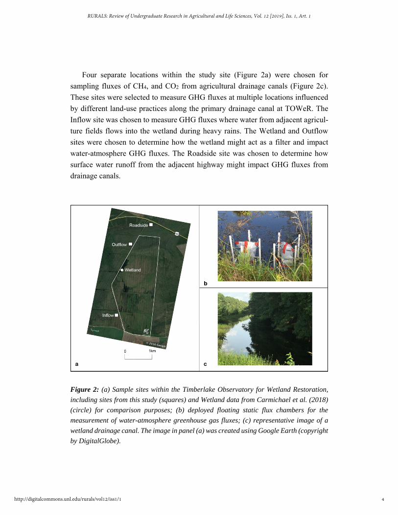
Four separate locations within the study site (Figure 2a) were chosen for

sampling fluxes of CH4, and CO2 from agricultural drainage canals (Figure 2c).

These sites were selected to measure GHG fluxes at multiple locations influenced

by different land-use practices along the primary drainage canal at TOWeR. The

Inflow site was chosen to measure GHG fluxes where water from adjacent agricul-

ture fields flows into the wetland during heavy rains. The Wetland and Outflow

sites were chosen to determine how the wetland might act as a filter and impact

water-atmosphere GHG fluxes. The Roadside site was chosen to determine how

surface water runoff from the adjacent highway might impact GHG fluxes from

drainage canals.

Figure 2: (a) Sample sites within the Timberlake Observatory for Wetland Restoration,

including sites from this study (squares) and Wetland data from Carmichael et al. (2018)

(circle) for comparison purposes; (b) deployed floating static flux chambers for the

measurement of water-atmosphere greenhouse gas fluxes; (c) representative image of a

wetland drainage canal. The image in panel (a) was created using Google Earth (copyright

by DigitalGlobe).

4



Site mesoclimate and environmental measurements

Environmental variables were continuously measured at each sampling location

(Figure 2a) in July 2016 and compared to historical data from the State Climate

Office of North Carolina’s Climate Retrieval and Observations Network of the

Southeast (CRONOS) Database monitoring station #311949 located within 2 km

of TOWeR in the Gum Neck Community of Tyrrell County, North Carolina. Air

temperature and relative humidity were measured continuously at 2m above ground

using a HOBO Pro V2 sensor and data logger (Model U23–001, Onset, Bourne,

MA) shielded from direct sunlight and the nighttime sky.

Daily water quality measurements were taken in the wetland at each site as

described in Carmichael & Smith (2016). Salinity was monitored using a YSI

EcoSense EC300A portable conductivity, salinity, and temperature meter (YSI,

Yellow Springs, OH). Surface water pH was monitored using a YSI EcoSense

pH100A portable pH, mV, and temperature meter. All instruments were calibrated

in the field prior to measurements. In addition to mesoclimate and water quality

measurements, and water depth at each site was measured (Carmichael et al., 2018).

Water-atmosphere greenhouse gas fluxes

Water-atmosphere GHG fluxes were measured using a static chamber

approach, following a protocol previously used at TOWeR (Carmichael et al., 2018;

Helton et al., 2014). Floating static flux chambers (Figure 2b) were constructed

from 10L gas sampling bags as described in detail in Helton et al. (2014). Static

flux chambers were deployed at three sites (Inflow, Outflow, and Roadside) at

TOWeR (Figure 2a) over a 24 h period in July 2016. Data for the Wetland site are

included in this manuscript with permission from Carmichael et al. (2018) for

comparison. At the beginning of each sampling interval, air temperature,

barometric pressure, and wind speed were recorded using a Kestrel 4000 weather

and environmental meter (Kestrel Instruments, Boothwyn, PA). Triplicate 10 mL

gas samples were collected from each chamber as described in Helton et al. (2014)

and Carmichael et al. (2018) at three time points over a 24 h incubation: 0, 8, and

24 hours.

5



Gas analyses

All gas samples were stored at room temperature for less than one week before

analysis via gas chromatography at the Duke River Center. Gas samples were ana-

lyzed for CO2 and CH4 concentrations at the Duke River Center following the

protocol outlined in Carmichael et al. (2018), Carmichael & Smith (2016), Helton

et al. (2014), and Morse et al. (2012). Samples were injected by a Tekmar 7050

Headspace Autosampler into a Shimadzu 17A gas chromatograph with an electron

capture detector and flame ionization detector (Shimadzu Scientific Instruments,

Columbia, MD) retrofitted with six-port valves and a methanizer to allow the

determination of the three gases from the same sample. Ultra-high purity N2 was

used as the carrier gas, and a P5 mixture served as the make-up gas for the electron

capture detector. A Nafion tube (Perma Pure, Toms River, NJ) and counter-current

medical breathing air were used to remove water vapor from the sample stream.

Gas concentrations were determined by comparing the peak areas of samples and

certified primary standards (range of standards 100–10,000 μL L−1 for CO2 and

0.3–5000 μL L−1 for CH4; Airgas, Morrisville, NC) using GCsolution software

(Shimadzu Scientific Instruments).

Water-atmosphere greenhouse gas flux calculations

Under ideal conditions in a static chamber incubation, gases either accumulate

or are consumed linearly over time (Livingston & Hutchinson, 2009); GHG fluxes

are determined by regression analysis of the change in gas concentration over time

in the chamber. Static flux chambers are sensitive to disturbance, so rigorous

quality control measures (see description below) must be applied. Measured gas

concentrations were initially converted from ppmv to μg m−3 using the ideal gas

law and field measurements of air temperature and barometric pressure. Quality

control measures, as described in detail in Carmichael et al. (2018), Helton et al.

(2014), and McInerney & Helton (2016), were then applied to the data set.

For GHG flux calculations, we began by calculating the average of all sample

replicates that were within 10% of one another (McInerney & Helton, 2016). Next,

these values were used to calculate the minimum detectable concentration

difference (MDCD) for each sampling date (Yates et al., 2006). Incubations that

did not exceed the MDCD were excluded from the analysis. Gas fluxes are reported

6



as a flux per unit exchanging surface area. Therefore, some additional transfor-

mations were required before regression analyses could be completed (Carmichael

et al., 2018). In calculating water-atmosphere fluxes, the volume to surface area

ratio of the static flux chambers obtained by Helton et al. (2014) was used for con-

versions. Once these conversions were completed, linear regression was used to

calculate GHG fluxes. An incubation met the assumption of linearity when r2 >

0.85; all incubations below this value were discarded from the analysis (Carmichael

et al., 2018).

Statistical analyses

Data were tested for normality using a Shapiro-Wilk test. A one-way analysis

of variance was then used to compare GHG fluxes among sites (threshold for sig-

nificance, P<0.05). When necessary, multiple comparisons were conducted using

Tukey-Kramer HSD tests. Statistical analyses were completed using Sigma Plot v.

12 (Systat Software, San Jose, CA).

3. Results

Site mesoclimate and environmental measurements

Mesoclimate data indicate that the daily temperature profile in July 2016 was

similar to both the 10-year weather averages (average maximum daily temperature,

30.77±1.99°C; average daily temperature, 25.90±2.08°C; average minimum daily

temperature, 21.02±2.37°C) and the 30-year climate normal (average maximum

daily temperature, 30.67°C; average daily temperature, 25.50°C; average minimum

daily temperature, 20.28°C) for Tyrrell County, North Carolina. Fresh surface

water conditions (salinity = 0.1 ± 0.0 ppt) and relatively constant surface water pH

(pH = 4.69 ± 0.07) were maintained throughout the study period. Mean surface

water depth at the Inflow, Outflow, Roadside, and Wetland were 0.42 ± 0.01 m

(range, 0.39 - 0.44 m), 1.2 ± 0.2 m (range, 0.8 - 1.7 m), 0.37 ± 0.05 m (range, 0.24

- 0.51 m), and 0.31 ± 0.03 m (range, 0.19 - 0.45 m) respectively.

7



Water-Atmosphere greenhouse gas fluxes

The mean water-atmosphere GHG fluxes at the Inflow, Outflow, and Roadside

ranged from 144.1 ± 11.6 - 189.3 ± 33.4 mg CO2 m-2h-1 and 3.1 ± 0.6 - 12.1 ± 6.2

mg CH4 m-2h-1 (Figure 3). For CO2, there was no significant difference in water-

atmosphere fluxes between the Inflow, Outflow, and Roadside; however, all sites

had significantly lower fluxes of CO2 when compared to the Wetland (P<0.001).

For CH4, the only significant difference was between the Roadside and Wetland,

with the Wetland site having a significantly larger flux (ca. 10×, P<0.05). The

Inflow, Outflow, and Roadside were statistically indistinguishable.

Figure 3: Water-atmosphere greenhouse gas fluxes of CO2 (a) and CH4 (b). Asterisks

indicate a significant difference between the mean greenhouse gas flux at a given sample

site compared to the Wetland. Error bars represent standard error.

4. Discussion

GHG fluxes across the water-atmosphere interface have historically been

understudied (Bastviken et al., 2004; Stanley et al., 2016). In this study, GHG emis-

sions were measured across the water-atmosphere interface in agricultural drainage

canals, a form of cryptic wetland that is common in cropland of low-lying coastal

8



regions. Data from this study show that including agricultural drainage canals in

the measured GHG fluxes from TOWeR increases site CO2 and CH4 emissions by

ca. 1% each.

Greenhouse gas fluxes from TOWeR

The present study augments the existing pool of research regarding GHG

fluxes from TOWeR across the three primary pathways of gas exchange in wet-

lands: the water-atmosphere, sediment-atmosphere, and plant-atmosphere inter-

faces. GHG flux via the water-atmosphere interface at TOWeR was previously

studied by Carmichael et al. (2018) and Helton et al. (2014). As stated before, GHG

flux data from Carmichael et al. (2018) was used as a point of comparison for the

drainage canal fluxes reported in the present study. In Helton et al. (2014), a site

located upstream of the Inflow site in this study received a high concentration of

agricultural runoff and was found to have consistent CH4 fluxes of < 8 mg m-2 h-1

between May and October 2012. The Inflow site of the present study had a stronger

CH4 flux of 12.1 ± 6.2 mg m-2 h-1. Helton et al. (2014) did not report values for CO2

fluxes.

GHG flux across the sediment-atmosphere interface at TOWeR was studied by

Morse et al. (2012). Data from sites within the regularly flooded portion of the

restored wetland showed mean GHG fluxes of 150 mg CO2 m-2 h-1 and 1.2 mg CH4

m-2 h-1 (Morse et al., 2012). While the present study reports similar CO2 fluxes to

Morse et al. (2012), CH4 exchanges in this study appear to be stronger than those

across the sediment-atmosphere interface.

GHG exchanges via standing dead trees, a pathway of gas flux across the plant-

atmosphere interface, were studied by Carmichael et al. (2018), with results show-

ing a mean CH4 flux of 0.4 ± 0.1 mg m-2 h-1 and a mean CO2 flux of 114.6 ± 23.8

mg m-2 h-1. A comparison of data from Carmichael et al. (2018) to data from the

present study indicates that CH4 and CO2 fluxes across the water-atmosphere inter-

face at TOWeR represent the larger source of these GHGs to the atmosphere.

Results indicate that taking CO2 and CH4 fluxes from agricultural drainage

canals into account during the calculation of total GHG flux from TOWeR

increases site CO2 and CH4 emissions by ca. 1% each. Thus, including GHG fluxes

9



from these cryptic wetlands is an important consideration in calculating total GHG

emissions from the site.

Patterns in water-atmosphere greenhouse gas fluxes at TOWeR

In this study, CH4 and CO2 fluxes from the drainage canal sites were lower than

those from the Wetland. This disparity most likely stems from differences in vege-

tation, C quality, and sediment decomposition rates between these sites. The drain-

age canals at TOWeR lack abundant aquatic vegetation, which has been shown to

increase the availability of high-quality carbon substrates in wetland sediments

(Fonesca et al., 2017). This high-quality C can be classified as labile organic matter,

which is more readily decomposed by sediment microbial communities (Barré et

al., 2016), thus stimulating decomposition pathways and the evolution of CO2 and

CH4 (Corteselli et al., 2017). In fact, higher CH4 fluxes have been observed in veg-

etated drainage ditches compared to those that lack vegetation (Schrier-Uijl et al.,

2010; Schrier-Uijl et al., 2011). Thus, the presence of vegetation in the wetland

proper likely increased C-gas emissions, as compared to the sparsely-vegetated

agricultural drainage canals.

Among the three drainage canal sites, the Inflow showed the greatest CO2 and

CH4 emissions. Although we did not measure porewater concentrations of nitrogen

(N) and phosphorous (P) in this study, the observed trend might be explained by

the proximity of the Inflow site to agricultural runoff containing nutrients. Studies

have shown that additions of specific amounts of N and P to water can lead to

increased CH4 emissions, especially in the presence of carbon (Kim et al., 2015).

Juutinen et al. (2018) found that CH4 flux in peatlands increased with the addition

of an N/P/K fertilizer. However, N and P additions to soil have also shown widely

varying effects on CH4 evolution, including stimulation of CH4 oxidation, a process

which may result in decreased CH4 fluxes to the atmosphere (Veraart et al., 2015).

Similarly, the response of soil respiration (i.e. CO2 flux) to nutrient addition is

highly variable and inconsistent both spatially and temporally (Cleveland & Town-

send, 2006; and as reviewed in Schlesinger & Andrews, 2000 and Raich &

Schlesinger, 1992).

10



Conclusions

Cryptic wetlands have traditionally been understudied (Yavitt, 2010), though

recent experimental evidence indicates the importance of including these wetlands

in predictive models of ecosystem carbon-dynamics (Ullah & Moore, 2011;

Martinson et al., 2010; Creed et al., 2003). In this study, including GHG fluxes

from one type of cryptic wetland (i.e. previously-omitted agricultural drainage

infrastructure) in the calculation of total GHG fluxes from TOWeR increased site-

based CO2 and CH4 fluxes. Although the localized spatial footprint of agricultural

drainage infrastructure may be individually small, the collective impact of these

human-engineered systems has the potential to be large, particularly in low-lying

regions (i.e. < 2 m elevation) where land use is dominated by agriculture. As such,

there is a need to further elucidate the processes and dynamics that influence GHG

emissions from these cryptic wetland environments.

5. References

Ardón, M., Morse, J. L., Doyle, M. W., & Bernhardt, E. S. (2010). The water quality

consequences of restoring wetland hydrology to a large agricultural watershed in the

southeastern coastal plain. Ecosystems, 13, 1060-1078.

Barré, P., Plante, A. F., Cécillon, L., Lutfalla, S., Baudin, F., Bernard, S., . . . Chenu, C.

(2016). The energetic and chemical signatures of persistent soil organic matter.

Biogeochemistry, 130, 1-12.

Bastviken, D., Cole, J., Pace, M., & Tranvik, L. (2004). Methane emissions from lakes:

dependence of lake characteristics, two regional assessments, and a global estimate.

Global Biogeochemical Cycles, 18, GB4009.

Carmichael, M. J., Bernhardt, E. S., Bräuer, S. L., & Smith, W. K. (2014). The role of

vegetation in the annual flux of methane to the atmosphere: should vegetation be

included as a distinct category in the global methane budget? Biogeochemistry, 119, 1-

24.

Carmichael, M. J., Helton, A. M., White, J. C., & Smith, W. K. (2018). Standing dead trees

are a conduit for the atmospheric flux of CH4 and CO2 from wetlands. Wetlands, 38,

133-143.

Carmichael, M. J., & Smith, W. K. (2016). Standing dead trees: a conduit for the

amospheric flux of greenhouse gases from wetlands? Wetlands, 36, 1183-1188.

11



Carter, L. J. (1975). Agriculture: a new frontier in coastal North Carolina. Science, 189,

271-275.

Chanton, J. P., Martens, C. S., & Kelley, C. A. (1989). Gas transport from methane-

saturated, tidal freshwater and wetland sediments. Limnology and Oceanography, 34,

807-819.

Clements, W. E., & Wilkening, M. H. (1974). Atmospheric pressure effects on 222Rn

transport across the Earth-air interface. Journal of Geophysical Research, 79, 5025-

5029.

Cleveland, C. C., & Townsend, A. R. (2006). Nutrient additions to a tropical rain forest

drive substantial soil carbon dioxide losses to the atmosphere. Proceedings of the

National Academy of Science, 103, 10316-10321.

Corteselli, E. M., Burtis, J. C., Heinz, A. K., & Yavitt, J. B. (2017). Leaf litter fuels

methanogenesis throughout decomposition in a forested peatland. Ecosystems, 20,

1217-1232.

Cowardin, L. M., Carter, V., Golet, F. C., & LaRoe, E. T. (1979). Classification of wetlands

and deepwater habitats of the United States. United States Fish and Wildlife Service,

FWS/OBS-79/31, 47.

Creed, I.F., Sanford, S.E., Beall, F.D., Molot, L.A., & Dillon, P.J. (2003) Cryptic wetlands:

integrating hidden wetlands in regression models of the export of dissolved organic

carbon from forested landscapes. Hydrological Processes, 17, 3629-3648.

Davidson, E. A., Ishida, F. Y., & Nepstad, D. C. (2004). Effects of an experimental drought

on soil emissions of carbon dioxide, methane, nitrous oxide, and nitric oxide in a moist

tropical forest. Global Change Biology, 10, 718-730.

FAO. FAOSTAT. Agri-Environmental Indicators (Land Use). (Latest Update: December

13, 2017). Accessed July 26, 2018. URI: http://faostat3.fao.org/

Fonesca, A. L. d. S., Marinho, C. C., & Esteves, F. d. A. (2017). Potential methane

production associated with aquatic macrophytes detritus in a tropical coastal lagoon.

Wetlands, 37, 763-771.

Helton, A. M., Bernhardt, E. S., & Fedders, A. (2014). Biogeochemical regime shifts in

coastal landscapes: the contrasting effects of saltwater incursion and agricultural

pollution on greenhouse gas emissions from a freshwater wetland. Biogeochemistry,

120, 133-147.

Joabsson, A., Christensen, T. R., & Wallén, B. (1999). Vascular plant controls on methane

emissions from northern peatforming wetlands. TRENDS in Ecology and Evolution,

14, 385-388.

12



Juutinen, S., Moore, T. R., Bubier, J. L., Arnkil, S., Humphreys, E. R., Marincak, B., . . .

Larmola, T. (2018). Long-term nutrient addition increased CH4 emission from a bog

through direct and indirect effects. Scientific Reports, 8, Article number 3838.

Kim, S. Y., Veraart, A. J., Meima-Franke, M., & Bodelier, P. L. E. (2015). Combined

effects of carbon, nitrogen and phosphorus on CH4 production and denitrification in

wetland sediments. Geoderma, 259-260, 354-361.

Livingston, G. P., & Hutchinson, G. L. (2009). Enclosure-based measurement of trace gas

exchange: applications and sources of error. In P. A. Matson & R. C. Harriss (Eds.),

Biogenic trace gases: measuring emissions from soil and water (pp. 14-51).

Cambridge, Massachusetts: Wiley-Blackwell.

Martinson, G. O., Werner, F. A., Scherber, C., Conrad, R., Corre, M. D., Flessa, H., . . .

Veldkamp, E. (2010). Methane emissions from tank bromeliads in neotropical forests.

Nature Geoscience, 3, 766-769.

Mattson, M. D., & Likens, G. E. (1990). Air pressure and methane fluxes. Nautre, 347,

718-719.

McInerney, E., & Helton, A. M. (2016). The effects of soil moisture and emergent

herbaceous vegetation on carbon emissions from constructed wetlands. Wetlands, 36,

275-284.

Morse, J. L., Ardón, M., & Bernhardt, E. S. (2012). Greenhouse gas fluxes in southeastern

U.S. coastal plain wetlands under contrasting land uses. Ecological Applications, 22,

264-280.

Myhre, G., Shindell, D. T., Breon, F.-M., Collins, W., Fuglestvedt, J., Huang, J., . . . Zhang,

H. (2013). Anthropogenic and Natural Radiative Forcing. In T. F. Stocker, D. Qin, G.-

K. Plattner, M. Tignor, S. K. Allen, J. Boschung, A. Nauels, Y. Xia, V. Bex, & P. M.

Midgley (Eds.), Climate Change 2013: The Physical Science Basis. Contribution of

Working Group I to the Fifth Assessment Report of the Intergovernmental Panel on

Climate Change. Cambridge, UK New York, NY: Cambridge University Press.

Needham, R. (2006). Implementation plan for agricultural restoration at Timberlake

Farms. Needham Environmental incorporated, Wilmington, North Carolina.

Poindexter, C. M., Baldocchi, D. D., Matthes, J. H., Knox, S. H., & Variano, E. A. (2016).

The contribution of an overlooked transport process to a wetland's methane emissions.

Geophysical Research Letters, 43, 6276-6284.

Raich, J.W., & Schlesinger, W.H. (1992) The global carbon dioxide flux in soil respiration

and its relationship to vegetation and climate. Tellus, 44B, 81-99.

13



Rusch, H., & Rennenberg, H. (1998). Black alder (Alnus glutinosa (L.) Gaertn.) trees

mediate methane and nitrous oxide emission from the soil to the atmosphere. Plant and

Soil, 201, 1-7.

Schimel, J. P. (1995). Plant transport and methane production as controls on methane flux

from arctic wet meadow tundra. Biogeochemistry, 28, 183-200.

Schlesinger, W.H., & Andrews, J.A. (2000) Soil respiration and the global carbon cycle.

Biogeochemistry, 48, 7-20.

Schlesinger, W. H., & Bernhardt, E. S. (2013). Biogoechemistry: An Analysis of Global

Change (3 ed.). Waltham, MA: Elsevier.

Schütz, H., Schröder, P., & Rennenberg, H. (1991). Role of plants in regulating the

methane flux to the atmosphere. In T. D. Sharkey, E. A. Holland, & H. A. Mooney

(Eds.), Trace Gas Emissions by plants (pp. 29-63). New York: Academic Press, Inc.

Stanley, E. H., Casson, N. J., Christel, S. T., Crawford, J. T., Loken, L. C., & Oliver, S. K.

(2016). The ecology of methane in streams and rivers: patterns, controls, and global

significance. Ecological Monographs, 86, 146-171.

Strack, M., & Zuback, Y. C. A. (2013). Annual carbon balance of a peatland 10 yr

following restoration. Biogeosciences, 10, 2885-2896.

Titus, J. G., & Richman, C. (2001). Maps of lands vulnerable to sea level rise: modeled

elevations along the US Atlantic and Gulf coasts. Climate Research, 18, 205-228.

Ullah, S., & Moore, T.R. (2011) Biogeochemical controls on methane, nitrous oxide, and

carbon dioxide fluxes from deciduous forest soils in eastern Canada. Journal of

Geophysical Research, 116, G03010.

Veraart, A. J., Steenbergh, A. K., Ho, A., Kim, S. Y., & Bodelier, P. L. E. (2015). Beyond

nitrogen: the importance of phosphorus for CH4 oxidation in soils and sediments.

Geoderma, 259-260, 337-346.

Yates, T. T., Si, B. C., Farrell, R. E., & Pennock, D. J. (2006). Probability distribution and

spatial dependence of nitrous oxide emission: temporal change in hummocky terrain.

Soil Science Society of America Journal, 70, 753-762.

Yavitt, J. B. (2010). Cryptic wetlands. Nature Geoscience, 3, 749-750.

14



carbon dioxide (co2) and methane (ch4) fluxes from

Documents