NBER WORKING PAPER SERIES

CAREER PROGRESSION, ECONOMIC DOWNTURNS, AND SKILLS

Jerome AddaChristian Dustmann

Costas MeghirJean-Marc Robin

Working Paper 18832http://www.nber.org/papers/w18832

NATIONAL BUREAU OF ECONOMIC RESEARCH1050 Massachusetts Avenue

Cambridge, MA 02138February 2013

We are grateful for funding from the DfES through the Centre for Economics of Education and tothe ESRC through CEMMAP and the Centre for Fiscal Policy at the IFS. Costas Meghir thanks theESRC for funding through a Professorial Fellowship (RES-051-27-0204) as well as the Cowles foundationat Yale. JM Robin gratefully acknowledges financial support from the Economic and Social ResearchCouncil through the ESRC Centre for Microdata Methods and Practice grant RES-589-28-0001, andfrom the European Research Council (ERC) grant ERC-2010-AdG-269693-WASP. The views expressedherein are those of the authors and do not necessarily reflect the views of the National Bureau of EconomicResearch.

NBER working papers are circulated for discussion and comment purposes. They have not been peer-reviewed or been subject to the review by the NBER Board of Directors that accompanies officialNBER publications.

© 2013 by Jerome Adda, Christian Dustmann, Costas Meghir, and Jean-Marc Robin. All rights reserved.Short sections of text, not to exceed two paragraphs, may be quoted without explicit permission providedthat full credit, including © notice, is given to the source.

Career Progression, Economic Downturns, and SkillsJerome Adda, Christian Dustmann, Costas Meghir, and Jean-Marc RobinNBER Working Paper No. 18832February 2013JEL No. C15,C23,C33,I24,J01,J08,J22,J24,J3,J31,J6,J62

ABSTRACT

This paper analyzes the career progression of skilled and unskilled workers, with a focus on how careersare affected by economic downturns and whether formal skills, acquired early on, can shield workersfrom the effect of recessions. Using detailed administrative data for Germany for numerous birth cohortsacross different regions, we follow workers from labor market entry onwards and estimate a dynamiclife-cycle model of vocational training choice, labor supply, and wage progression. Most particularly,our model allows for labor market frictions that vary by skill group and over the business cycle. Wefind that sources of wage growth differ: learning-by-doing is an important component for unskilledworkers early on in their careers, while job mobility is important for workers who acquire skills inan apprenticeship scheme before labor market entry. Likewise, economic downturns affect skill groupsthrough very different channels: unskilled workers lose out from a decline in productivity and humancapital, whereas skilled individuals suffer mainly from a lack of mobility.

Jerome AddaDepartment of EconomicsEuropean University InstituteVilla San PaoloVia della Piazzuola 4350133 Firenze j.adda@ucl.ac.uk

Christian DustmannDepartment of EconomicsUniversity College LondonGower Street, London WC1E 6BT, UKc.dustmann@ucl.ac.uk

Costas MeghirDepartment of EconomicsYale University37 Hillhouse AvenueNew Haven, CT 06511and IZAand also NBERc.meghir@yale.edu

Jean-Marc RobinSciences PoDepartment of Economics(Office room, J402)28 rue des Saints Pères75007 Paris Francejeanmarc.robin@sciences-po.fr

1 Introduction

The early years in a worker’s career are essential, not only because wages rise most

rapidly, but also because workers may be most vulnerable to economic shocks and make

important choices about training and investment into human capital. Since these early

choices and events may have significant long-term career consequences, it is important

to understand their dynamics and effects, as well as the way they interact with shocks

to the overall economy.

One essential part of this early career progression is wage growth, which has been

seen as a consequence of investment in learning and human capital (see, e.g., Ben-Porath

(1967), Becker (1964), Rosen (1972), Rosen (1976))1, mobility and job shopping (see,

e.g, Mincer and Jovanovic (1981), Topel and Ward (1992)), or both (see, e.g., Gladden

and Taber (2000), Altonji, Smith, and Vidangos (2009), or Gladden and Taber (2009b)).

Although this literature provides important insights into worker’s wage progressions,

however, it offers little information about how early career progression is affected by

economic shocks, and how wage growth, transitions between jobs and into and out of

non-employment, and the economic cycle interact.2 Such a knowledge gap is surprising,

not only because youth unemployment is a major concern, but because recent research

highlights the potentially harmful effects that economic shocks at early ages may have

on workers’ careers (see, e.g., Oreopoulos, Von Wachter, and Heisz (2012)).

A related question is how the harmful effects of economic shocks on young workers’

careers can be minimized. It is possible, for instance, that skills acquired not on the

job but in specifically designed training schemes can help shield young workers from

adverse labor market shocks. The possibility that this type of training provision may

help lessen the impact of economic shocks on young workers is suggested by the milder

impact that the recent global recession has had on youth unemployment in countries with

well-developed firm-based vocational training schemes.3 To test this conjecture, however,

1See Lemieux (2006) for an assessment of estimating wage determination equations based on learningmodels.

2See also French, Mazumder, and Taber (2006) who emphasize this point and address it in a reducedform context.

3For instance, while the youth unemployment rate between 2007 and 2011 has increased in mostOECD countries, it has remained stable in Austria and Switzerland and has even decreased in Germany- all countries with a large structured apprenticeship system that trains young workers for particular

2

it is important to better understand the factors that determine wage growth, mobility,

and non-employment, as well as their relation to economic shocks, in a context that

allows young individuals the opportunity to obtain vocational training in a structured

apprenticeship program.

In this paper, we address this issue by asking two important questions: First, how

do workers’ careers progress after secondary school in a world where wages grow through

job shopping and on-the-job learning and workers have the initial choice to acquire

occupation-specific skills in a 2-3 year structured vocational training scheme. Second,

how do the career profiles of workers who have chosen to enroll in a vocational train-

ing scheme compare with the profiles of those who have not, and how are these profiles

affected by economic shocks that hit individuals at different career stages. Addressing

these questions will not only throw light on how early career apprenticeship programs

affect career progression - an issue under renewed scrutiny in the policy debates of many

countries - but also how early career vocational training may help alleviate the effects of

economic downturns on employment and the career progression of young workers.

To answer these questions, we develop a life cycle model of career choice and career

progression in which workers decide whether to acquire occupation-specific training after

secondary school and before entering the labor market or to join the labor market as

unskilled workers. We model this choice in accordance with the institutional features

in Germany, where almost four in five workers enter the labor market after secondary

school either directly as unskilled workers or indirectly as apprentices, who enroll in a

2 to 3-year structured, firm-based training scheme before entering the labor market as

skilled workers.4 The German system is unique in that it allows a precise distinction

between skilled (i.e., those who choose apprenticeship) and unskilled workers (i.e., those

who decide to join the labor market directly) in a homogeneous work environment in

which training decisions are made at the start of the career and skilled and unskilled

occupations after secondary school (OECD Labor Market Statistics 2012)4Apprenticeship training combines formal classroom teaching with on-the-job training by qualified

supervisors who implement a structured curriculum that leads to skill certification within a narrowlydefined occupation, such as bank clerk or plumber. Firm-based apprenticeship training schemes have anumber of advantages over vocational schools: craft techniques and customer interaction may be taughtmore effectively in a work environment than in the classroom, and firms may know better than schoolswhich skills are needed in the workplace. Firm-based training may also allow for smoother transitionsof firm-trained apprentices into employment (see Ryan, 2001 and Parey, 2009 for evidence).

3

workers do similar jobs.5

Our model allows for direct job-to-job mobility, as well as transitions into and out

of non-employment. We allow the key parameters that characterize search frictions to

differ across skill groups, over the experience profile, and, importantly, over the busi-

ness cycle. We model workers’ career progressions in a framework in which wages grow

because workers learn on the job and through job shopping. Our model thus draws on

models of education choice6 and wage determination.7 It also builds on the empirical

labor literature, endowing the wage equation with a rich stochastic structure in which

wages grow with experience and job-(firm-)specific tenure and depend on a match-specific

component as in Wolpin (1992).8 The wage equations are specific to the two alterna-

tive careers (skilled or unskilled) as in a Roy type model. In the presence of search

frictions, these careers could differ in rates of job arrival, job destruction, and mobility.

For example, if occupation-specific apprenticeship training reduces flexibility because of

training specificity, the job arrival rates should be lower for apprentices and lead to longer

unemployment spells.9 Our framework also draws on the macro labor literature by allow-

ing both aggregate shocks and labor market transitions to affect relative wages between

the two groups (see Barlevy (2002), Nagypal (2005), Petrongolo and Pissarides (2008)

or Shimer (2012)). Our model thus enables assessment of the business cycles effect on

labor market attachment, experience, and job mobility, with a particular emphasis on

heterogeneous effects across skill groups and at various stages of a career.

Our analysis is based on unique administrative data drawn from social security

records, which allows us to track the careers and wages of individuals from their en-

try to the labor market onwards. These data also provide precise records of the training

choices individuals make after labor market entry. The high quality of these data is an

5There is a large overlap in occupations for workers who enter the labor market directly after secondaryschool and those who train in an apprenticeship scheme.

6See, e.g., Card (1999), Taber (2001), Card (2001), Cameron and Heckman (1998).7See, e.g., papers by Willis and Rosen (1979), Heckman and Sedlacec (1985), Altonji and Shakotko

(1987), Topel (1991), Altonji and Williams (1998), Altonji and Williams (2005), Parent (1999), Dust-mann and Meghir (2005).

8For recent contributions on wage dynamics, see, for example, Meghir and Pistaferri (2004), Low,Meghir, and Pistaferri (2010) and Altonji, Smith, and Vidangos (2009). Sullivan (2010) and Pavan(2011) study wages in a structural context that allows agents to choose between occupations.

9See, e.g., Heckman (1993). See also Fitzenberger and Kunze (2005), who investigate whether thislock-in effect explains part of the gender wage gap in Germany.

4

important strength of our approach: they accurately record all wages, shifts between dif-

ferent jobs, and transitions between non-employment and work, enabling us to precisely

assign wages to firms. Our sample covers men from what used to be West Germany, born

between 1960 and 1972 and observed from 1975 until 2004, a period that encompasses

three decades and many entry cohorts. Our data therefore allow us to compare the ca-

reers of individuals who enter the labor market faced with effectively different economic

conditions and training costs because of the varying availability of skilled training and

different opportunity costs of training. They thus provide exogenous variation that al-

lows us to identify initial choices of whether to enroll in apprenticeship training or enter

the labor market directly, which we combine with a dynamic model that characterizes

apprenticeship and non-apprenticeship careers. The data also reflect variations in the

economic cycle that expose workers to recessions at various stages of their careers.

We find that, at an early career stage, the careers of individuals who choose to acquire

apprenticeship training at labor market entry (hereafter, skilled workers) differ markedly

from those who do not (”unskilled” workers). Those who undergo training enter the labor

market with far higher wages, while those who enter as unskilled workers undergo a period

of rapid wage growth during the first 5 years in the labor market. Remarkably, this wage

growth during the early career phase is due primarily to on-the-job learning and to a far

lesser extent, to job shopping. Also interesting are the differences in the fundamental

parameters that drive wage progressions for these two groups: whereas unskilled workers

have higher job destruction rates than skilled workers, they also have higher job arrival

rates, both on and off the job. Although these differences narrow over the career, they

never converge, a surprising observation given that individuals are fairly homogeneous

before making their training choice and compete for similar jobs.

These differences in the underlying parameters, which are greater in the early career

stages, lead to surprising differences in the way skilled and unskilled workers respond to

economic shocks. Evaluating the long-run effect of a recession, we find that economic

shocks have permanent effects on human capital for both unskilled and skilled workers.

Nonetheless, the career stage at which a recession hits is important: economic shocks at

an early stage in a career have larger consequences on accumulated work experience than

5

at a later stage. We then investigate whether these shocks to employment translate into

wages. We find that exposure to an economic shock early in a worker’s career leads to

wage reductions that persist for 5 to 10 years. However, the wage differential between

skilled and unskilled workers is smaller than human capital would suggest, a result of the

dramatic differences in recession-induced job mobility. Whereas skilled workers tend to

remain with the same firm, unskilled workers are more mobile and compensate for the

loss in human capital through the accumulation of search capital.

By identifying precise channels through which workers’ careers are affected by eco-

nomic shocks, our model contributes to an important and growing recent literature on

the effect of economic shocks on workers (see, e.g., Ruhm (1991), Jacobson, LaLonde,

and Sullivan (1993), Oddbjorn and Roed (2006), Davis and von Wachter (2011), or Ore-

opoulos, Von Wachter, and Heisz (2012)). These earlier studies, however, although they

provide interesting insights into the possibly devastating effects of economic shocks on

workers’ careers, do not distinguish between job destruction caused by economic reces-

sion and job destruction that would have happened anyway. Moreover, in any analysis

based on DiD type identification strategies, longer term projections may be confounded

by other economic shocks. Our analysis, in contrast, while supporting the key findings

of these papers, extends the literature by distinguishing recession effects from job sep-

arations that would have occurred anyway, by isolating the impact of a past shock on

future careers from other possible determinants, and by comparing the career impacts of

shocks that hit workers at different career stages.

Our paper also contributes to a better understanding of training schemes that develop

workplace-related vocational skills, schemes that are (once again being) recognized as a

key factor in strengthening competitiveness and growth.10 A crucial question for assessing

such schemes, however, is how they affect workers’ productivity and employment patterns.

Yet although the literature estimates the effects of apprenticeship training on wages11 and

10See, e.g., President Obama’s ”manufacturing skill speech” (http://www.whitehouse.gov/the-press-office/2011/06/08/president-obama-and-skills-americas-future-partners-announce-initiatives ) orthe British Governments renewed emphasis on firm-based apprenticeship programs (see the UK 2011budget (http://cdn.hm-treasury.gov.uk/2011budget complete.pdf ) and its allotment of an additional£180 million for up to 50,000 additional apprenticeship places.

11See, e.g., Winkelmann (1996) and Fersterer and Winter-Ebmer (2003), who report OLS estimatesfor the wage returns to apprenticeship training in Germany and Austria of around 15-20 percent, andFersterer, Pischke, and Winter-Ebmer (2008), who report IV estimates of 2.5 and 4 percent per year of

6

provides important insights into the returns to enrollment in vocational training schemes,

its focus on the wage component ignores the role of endogenous experience profiles and

the effects of selection into work (e.g., on life cycle earnings through employment). Not

only are these factors likely to be very important in any career comparison of skilled

and unskilled workers, they may interact differently with aggregate shocks for skilled

versus unskilled workers. Our contribution, therefore, is to provide a more detailed

understanding of the various channels that lead to higher returns for workers who undergo

apprenticeship training, a key factor in assessing whether such training schemes should

be encouraged in other countries.

The remainder of the discussion is structured as follows. Section 2 describes the

data set, outlines the institutional features, and provides descriptive statistics. Section 3

defines the model, section 4 explains our estimation method, and section 5 reports our

results. Section 6 concludes the paper.

2 Background and Data

In this section, we give some brief description about training choices and the firm based

apprenticeship system we are analyzing in this paper. We then describe our data and

sample, and provide some descriptive statistics.

2.1 The Apprenticeship System

The German Apprenticeship System is a vocational training programme which combines

on-the-job training, provided by the firm, with school education, provided and funded by

the state. Similar systems operate in Austria and Switzerland. The system offers training

in more than 500 white- and blue collar occupations 12. In practise, individuals choose

from a fairly small number of training professions. For instance, in our data, 70 percent

of all male apprentices are concentrated in 20 three digit occupations, with slightly more

than two-third of those being blue collar ones.

Apprenticeship training typically starts after secondary school, at around the age of

16, and lasts for 2 to 3 years. Germany tracks children after the age of 10 in lower,

training .12See http://berufenet.arbeitsagentur.de/berufe/index.jsp. for details.

7

intermediate and upper secondary schools. Pupils who attend lower and intermediate

secondary schools typically enroll in blue or white collar apprenticeship schemes. Pupils

who attend upper secondary schools are entitled to enroll directly into university.13

Apprenticeship training is highly structured, with a well-defined curriculum. It takes

place at the workplace for 3-4 days a week, under the supervision of qualified instructors,

where practical and workplace related knowledge is acquired, and at vocational state

schools for 1-2 days a week, where more general and academic knowledge, as well as the-

oretical knowledge specific to the chosen occupation is obtained. Both the practical and

the academic components are examined at the end of the training period, and successful

candidates obtain a professional qualification. We refer the reader to Steedman, Gospel,

and Ryan (1998) for more details.

2.2 Data and Sample

Our main data is a 2 percent sample of administrative social security records, covering

the years between 1975 and 2004, and made available by the German Institute for Em-

ployment Research. It records all spells of employed work of workers in the private and

public sectors, with exact dates when each job started and ended. The data does not

cover civil servants and the self employed. The data set reports the average daily pre-tax

wage at the end of each calendar year for ongoing employment spells. For individuals

who change firms within a calendar year, we observe the average wage from the begin-

ning of the calendar year or the employment spell (if it started after the beginning of the

calendar year) until the end of that spell. Thus wages are not averaged across different

firms. The wage data is top coded at the earnings limit for social security contributions.

For the sample we consider, this concerns only about 2.2 percent of all wage spells. We

take top coding into account in our estimation procedure, and we describe details below.

The data contains also information on the apprenticeship training period, and whether

a worker holds an apprenticeship qualification or not, as well as their overall educational

qualifications.

In our analysis, we focus on West-German men born in the period between 1960-1972,

who enter the labor market with a lower or intermediate secondary degree, which is not

13See Dustmann (2004) for a detailed description of the German school system.

8

sufficient for attending university directly, and which is typically obtained by the age

of 16. We select these cohorts to ensure that we only include individuals whom we can

observe at the start of their labor market career so that we avoid any initial conditions

problem.

We then define two groups: individuals who enroll in apprenticeship schemes for at

least 2 years and successfully complete their training (in what follows we refer to these

individuals as ”skilled”), and individuals who enroll for a shorter period, but do not

graduate, or do not enroll and enter the labor market directly (we refer to these as

”unskilled”).14

From this data, we construct a data set of quarterly spells, thus assuming that all

decisions are made on a quarterly basis. Whenever during a quarter multiple spells are

present (e.g. an employment and an unemployment spell), we assign to that quarter the

spell that covers the largest proportion of that quarter. When the individual does not

move firms and thus the wage we observe is an average over more than one quarter, we

treat this as a time aggregated wage where we do not observe the individual constituents

of this average. This time aggregation problem is fully accounted for during estimation,

as we explain later.

The data contains 38,018 individuals who enroll in an apprenticeship training scheme

after secondary school, and 4,392 individuals who join the labor market directly and

without further training. These are followed through time, quarter after quarter up until

2004; we have thus a total of 3,667,223 quarterly observations. Finally, to identify the

determinants of choices of school tracks at age 10, we use 69,084 individuals who follow

the vocational track and 10,608 who follow the academic track. We provide more detail

on the sample selection in Appendix A.

As mentioned above, there is a large overlap in terms of occupations for skilled and

unskilled workers. In our sample individuals are employed in 292 3-digit occupations

after labor market entry. Out of those, 19 occupations employ only unskilled workers

14As an alternative to firm-based apprenticeship training, some youth attend vocational schools, whichoffer classroom training for two to three years, with unpaid work experience, and lead to a certificateequivalent to a firm-based apprenticeship (see Parey (2009) for details). About 6 percent of our sampleundertakes qualifying training in these vocational schools. Wage profiles of those who went through firmbased training and vocational schools are almost identical. We add these to the group of skilled workers.

9

(and these employ just about 1 percent of all unskilled workers), and 53 occupations

employ only skilled workers (and these employ just 1.4 percent of all skilled workers).

2.3 Descriptive Analysis of the Data

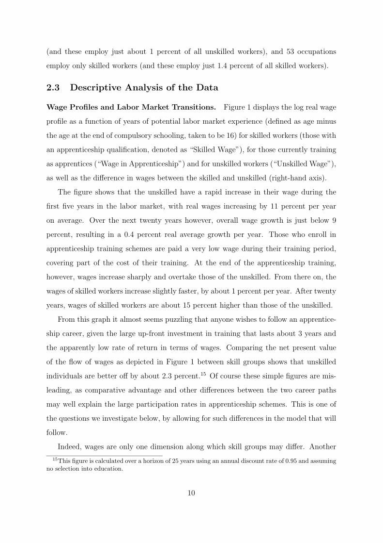
Wage Profiles and Labor Market Transitions. Figure 1 displays the log real wage

profile as a function of years of potential labor market experience (defined as age minus

the age at the end of compulsory schooling, taken to be 16) for skilled workers (those with

an apprenticeship qualification, denoted as “Skilled Wage”), for those currently training

as apprentices (“Wage in Apprenticeship”) and for unskilled workers (“Unskilled Wage”),

as well as the difference in wages between the skilled and unskilled (right-hand axis).

The figure shows that the unskilled have a rapid increase in their wage during the

first five years in the labor market, with real wages increasing by 11 percent per year

on average. Over the next twenty years however, overall wage growth is just below 9

percent, resulting in a 0.4 percent real average growth per year. Those who enroll in

apprenticeship training schemes are paid a very low wage during their training period,

covering part of the cost of their training. At the end of the apprenticeship training,

however, wages increase sharply and overtake those of the unskilled. From there on, the

wages of skilled workers increase slightly faster, by about 1 percent per year. After twenty

years, wages of skilled workers are about 15 percent higher than those of the unskilled.

From this graph it almost seems puzzling that anyone wishes to follow an apprentice-

ship career, given the large up-front investment in training that lasts about 3 years and

the apparently low rate of return in terms of wages. Comparing the net present value

of the flow of wages as depicted in Figure 1 between skill groups shows that unskilled

individuals are better off by about 2.3 percent.15 Of course these simple figures are mis-

leading, as comparative advantage and other differences between the two career paths

may well explain the large participation rates in apprenticeship schemes. This is one of

the questions we investigate below, by allowing for such differences in the model that will

follow.

Indeed, wages are only one dimension along which skill groups may differ. Another

15This figure is calculated over a horizon of 25 years using an annual discount rate of 0.95 and assumingno selection into education.

10

important dimension is labor market attachment. Figure 2 shows the proportion of

individuals who are in work as a function of age.16 It is apparent from the figure that

labor market attachment of skilled workers is stronger than that of the unskilled, with

a higher fraction of the skilled working at any age. The difference in the proportion of

individuals working narrows from about 10 percent at age 25 to 5 percent around age 40.

In Table 1 we report in more detail the transitions of the two skill groups between

the different states. The table displays the quarterly transition probabilities by skill

status and time in the labor market, which starts when the individual has found a first

job or an apprenticeship training scheme. The figures show that unskilled workers have

a higher probability of dropping out of work. During the first five years in the labor

market, each quarter, about 3 percent of employed skilled workers exit, while this figure

is about 9 percent for the unskilled. This proportion decreases when we focus on more

senior workers, and the difference between the two groups narrows. The figures in Table 1

also reveal that skilled individuals have a higher probability to return to work from non-

employment. For instance, for workers with 5 to 10 years of potential experience, 19

percent of skilled unemployed individuals find a job from one quarter to the next. For

the unskilled this figure is only 7 percent. Further, the probability of job to job transitions

is higher at the beginning for the unskilled, but declines after five years for both groups

and becomes marginally higher for the skilled.

To summarize, these figures indicate that - overall - the unskilled spend less time

working. Over a 25 years period, they work a total of 21.9 years, compared with a total

of 22.5 years for skilled workers. If we combine labor market participation and wages,

using a replacement rate of 40 percent when unemployed, we find that skilled individuals

are two percent better off in terms of net present value when they first enter the labor

market; this number increases to 5 percent if we assign zero earnings to unemployed

workers. Hence, the decision to obtain apprenticeship training cannot be assessed solely

on the basis of the implied earnings advantage as depicted in Figure 1. Another important

dimension of this choice is the employment prospect.

Figure 3 plots the number of firms in which an individual have been employed, where

16Germany has a compulsory military draft system during the period we consider, and we have elim-inated interruptions that are due to military service while constructing the figure.

11

the horizontal axis carries potential experience. It is evident from this figure that the

unskilled are more mobile during the first few years in the labor market. Thus, job

shopping can be an important source of the large initial wage growth for unskilled workers,

as we illustrate in Figure 1. To investigate this further, we decompose wage growth

into within and between firm wage growth and plot it against potential experience (see

Figure 4), distinguishing between the two skill groups. Between job wage growth is indeed

substantial, between 20 and 40 percent for the unskilled during the first 2-3 years in the

labor market, when skilled workers are still in the training phase. The gain in wages falls

over time, but is still large for both groups until about 5-7 years in the labor market,

with returns being close to zero after about 15 years. Within firm wage growth for the

the unskilled is likewise very high early on in the career reflecting the rapid learning that

takes place on the job. The equivalent training for the skilled takes place during the

training period (which we have not shown in the figure).

Figure 5 shows the path of residual wages for both skill groups over time, together

with the deviation of GDP from a trend. The residual wage is obtained by projecting

wages on age and regional dummies, so as to make individuals comparable across years.

We have also shaded the periods when GDP is below its trend, which we define as an

economic downturn. Our data encompasses three downturns, one in the mid-seventies, a

large one in the early eighties and one at the end of our sample, which starts in 2004. The

figure shows that wages are procyclical, with a correlation with GDP of 0.4 for unskilled,

and 0.57 for skilled workers. The precise mechanism that leads to such a correlation

is difficult to assess in a reduced form context. We return to this issue in detail in

Section 5.4.

3 The Model

We now turn to the description of the key features of our model, which is set in discrete

time, and where one period lasts one quarter. It focuses on individuals who leave sec-

ondary education at age 16 (and who chose the low or intermediate school track at age

10, see Section 2.1). At that point individuals have the choice either to enroll in an ap-

prenticeship scheme, or to enter the labor market as unskilled workers. Once this choice

12

has been made, individuals start their career. Throughout their work career, individuals

receive job offers with some probability, which may differ depending on whether they

are employed or not. Jobs can end either because of a quit or because of exogenous job

destruction. Wage growth occurs through several channels. It first depends on whether

individuals decide to train in a structured apprenticeship scheme, where wages are low

during the training period, but increase substantially after training is completed. Second,

we incorporate learning-by-doing, and we distinguish between general human capital and

firm-specific human capital. Finally, wages may grow through job mobility as we allow

for heterogenous worker-firm productivity matches. Individual choices include moving

between jobs when the opportunity arises and between work and unemployment as well

as the initial choice to undergo an apprenticeship. All these choices are made in order

to maximize the present value of future payoffs. Individuals derive utility from wages,

from benefits when out of work and from leisure. Those benefits are a function of the

wage earned in the last job in accordance with the benefit system in Germany. The

information set of agents consists of their skill status, their work experience, their tenure

on the job in the firm, their time invariant unobserved characteristics, the current value

of the productivity match with the firm, and the aggregate state of the economy. We

now describe relevant features of our model in more detail.

Aggregate shocks: We characterize the macroeconomic fluctuations of the economy

around the steady-state growth trend by de-trended GDP. The macro shock is relevant

because it potentially affects the relative price of the two skill groups as well as the

relative attractiveness of being out of work. It also affects the probability of finding a job

as well as the job destruction rate, in a way specific to both skill groups. This allows the

model to capture the different effect business cycles have on skilled and unskilled workers

along several dimensions, such as unemployment duration or job tenure, and which we

will explore later on. The macro state variable Gt is modeled as a discrete two-state

Markov process of order one. The transition probabilities are presented in Appendix C

in Table A1.

13

Wages and Matches: If a worker and a firm form a match at time t, the output is

split according to a rule that yields an annual wage wit to the worker. The way the split

is determined is not modeled here. Wage contracts are continuously updated following

shocks to match productivity, and, as in a standard Mortensen and Pissarides (1994)

model, really bad productivity shocks may result in unemployment.

Wages are modeled as follows. Let Si ∈ 0, 1 denote the worker’s apprenticeship

qualification status (1 for skilled and 0 for unskilled). Let Xit be the number of quarters

spent in work (including the apprenticeship period) since age 16.17 Let Tit denote the

number of quarters spent in the current job (Tit = 0 if the worker starts working in the

firm in period t). Let εi be a permanent individual characteristic that is unobserved by

the econometrician but is known by the worker and observed by the employer. Quar-

terly earnings wit are functions of the macroeconomic shock, Gt, skilled training, Si ,

experience, Xit, tenure, Tit, the unobserved permanent heterogeneity variable, εi, and a

match-specific component, κit:

lnwit = α0(εi) + αSSi + αX(Xit, Si) + αT (Tit, Si) + αG(Si)Gt + κit, (1)

where αX and αT are two skill-specific functions of experience and tenure. We use a

piecewise linear function, with nodes at 0, 2, 4, 6, 10 and 30 years of experience and

tenure. The specification is motivated by the fact that most of the non linearity in wage

profiles is early on, so we have a denser grid between 0 and 10 years of actual experience.

Unobserved heterogeneity affects the overall level of log wages and is discrete. This

specification is in line with the empirical evidence found in French, Mazumder, and

Taber (2006). They show that the return to experience appears to be unrelated to the

business cycle. The specification with an additive and separate unobserved productivity

term is consistent with findings in Gladden and Taber (2009a).

When the worker and the firm first meet (Tit = 0) they draw a match specific effect κi0

such that

κi0 ∼ N (0, σ20 (Si)) , (2)

which captures the heterogeneity in wages when individuals start a new job. We in-

17Xi,t+1 = Xit + 1 if the worker is working in period t; otherwise, Xi,t+1 = Xit. We do not allow fordepreciation of skills while unemployed.

14

terpret this as match specific heterogeneity and we allow it to differ by apprenticeship

status allowing us to estimate the extent to which job opportunities vary for skilled and

unskilled workers. In the empirical application we also distinguish between skilled work-

ers and those still in training to allow the innovation of the match component to be

different.18 Flinn (1986) shows the importance of worker-firm productivity matches to

explain the wage path of young workers. For subsequent periods within the firm, the

match component evolves as

κit = κit−1 + uit, (3)

uit ∼ iid N (0, σ2u(Si)). (4)

This allows for the possibility that the value of a match and the contracted wage can

change, while permitting persistence over time. Indeed, Topel and Ward (1992) show

that the match is close to a random walk. Contrary to the US and the UK, in Germany,

the cross sectional variance of wages does not increase over the lifecycle, which means

that a random walk of wages that continued across jobs would lead to counterfactual

implications and would be inappropriate. This led us to the above specification, where

the random walk component is reinitialized when changing jobs.

The utility of working and being out of work: Utility is assumed to take a log

form. In addition, we allow for a mobility cost or benefit µi when a worker moves between

jobs. This allows for the possibility that workers may move to a job that pays lower wages,

as is observed in the data. The one-off benefit/cost of moving is an iid random variable

µi such that

µi ∼ N (mµ(Si), σ2µ(Si)).

The instantaneous utility of work is therefore:

RWit ≡ RW (Si, Gt, Xit, Tit, κit, εi) = ln(wit) + µi ITit=0 (5)

where ITit=0 is an indicator variable equal to one for the first period of employment.

18Note that we are able to identify firm-worker productivity matches for those in training as we observewages during that period as well.

15

While unemployed, the individual derives a utility from unemployment benefits; these

are calculated as a fraction of the last wage when employed (denoted as wi(−1)), as in

the German unemployment insurance (UI) system that was in place over the period we

consider here. 19 In addition, there is a utility of leisure which varies across individuals

on the basis of their skills, experience, unobserved heterogeneity εi and a Gaussian white

noise ηit with variance σ2η. Thus, the instantaneous utility of unemployment is:

RUit ≡ RU(Si, Xit, wi(−1), ηit) = ln(γUwi(−1)) + γ(Xit, Si, εi) + ηit,

ηit ∼ iid N (0, σ2η(Si)),

(6)

with γU = 0.4 and where γ(Xit, Si, εi) is the utility of leisure, which is skill-specific, and

varies with unobserved heterogeneity (in a multiplicative way) and experience. The effect

of experience is modeled as a piecewise constant function (with nodes at 0, 2, 4, 6 and

30 years of experience).

Finally, we assume that all shocks κi0, uit, µi, ηit are jointly as well as serially

independent, and independent of the unobserved heterogeneity vector εi (see below for a

complete description of unobserved heterogeneity).

Transitions: Individual decisions to work, to move to a new job or to quit working are

carried out by comparing the lifetime values of each of these states.20 More specifically,

employed individuals may be laid off with probability δit ≡ δ(Gt, Si, Xit), which depends

on the state of the business cycle as well as experience and skill status. Exogenously

displaced individuals suffer a loss of their match specific effect which will lead on average

to lower wages upon re-entry, followed by a catch-up as the worker shop for better

matches. These facts are consistent with findings in Bender, Dustmann, Margolis, and

Meghir (2002) and von Wachter and Bender (2006). Conditional on not being laid off,

they draw an alternative job offer with probability πWit ≡ πW (Gt, Si, Xit). Unemployed

individuals draw a job offer with probability πUit ≡ πU(Gt, Si, Xit), which is a function

of the aggregate shock, skills and experience. They decide whether to take this job,

19When UI is exhausted (after about 18 months), an unemployed worker moves on to the means-testedunemployment assistance. Given the length of time for eligibility and the generosity of social assistancefor lower wage individuals, we have made the simplifying assumption that the replacement rate is always40 percent, which is on average correct for our population. Modeling the entire system would imply anincreased state space.

20The structure of the value functions is presented in appendix B.

16

depending on how the value of working compares to the value of unemployment. As

the business cycle affects both job arrival rates and layoffs, our model has some of the

features that are discussed in the macro labor literature (see for instance Davis and

Haltiwanger (1992), Barlevy (2002), Nagypal (2005), Petrongolo and Pissarides (2008)

or Shimer (2012)).

Training decision: The choice to enroll in apprenticeship training is assumed to be

a one-off decision made at age 16, and based on the comparison of the value of a career

under the two training alternatives, allowing for both the direct cost of training and

foregone earnings. We assume that both an unskilled job and an apprenticeship position

are available immediately. For simplicity, we refer to that decision as ”decision at age 16”,

although there is some heterogeneity in our sample, and in practise, we start modeling

from the point we see individuals joining the first job or an apprenticeship scheme.

The choice to become an apprentice is based on comparing the value of this decision

with the value of joining the labor market directly, minus the cost of the training decision,

which can be expressed as

V (Ωit|Si = 1)− costit > V (Ωit|Si = 0), (7)

where V (Ωit|S = j), j ∈ 0, 1 is the present value of payoffs, conditional on the state

variables at age 16 and the career chosen. At the start of the career, experience and

tenure are set to zero. The state vector Ωit contains also the business cycle state Gt

at that date, the match effect κi0 and mobility cost µi. The value of unskilled work

is conditioned on Ωit, which is also evaluated at zero experience and tenure, the same

business cycle shock, but with an offer from a different firm for an unskilled position.

This offer consists of a match effect κi0 and mobility cost µi.

The cost of training is modeled as:

costit = λR(Ri, Gt) + λ0(εi) + ωit, (8)

where λR(Ri, Gt), represents the (deterministic) direct costs of apprenticeship training,

which we allow to depend on the relative scarcity of apprenticeship training schemes

across time and regions (see e.g. Parey (2009) who illustrates the strong variation in

17

training schemes across regions in Germany). We proxy these by including interactions

between region of residence, Ri, and the state of the business cycle, Gt, both measured

when the choice is made at age 16. These interactions reflect how aggregate shocks affect

each of the eleven regions of (West) Germany. Such differential effects of GDP shocks

across regions will occur because industrial composition differs across regions or because

employment in some industries is more procyclical than in others. The availability of

data for thirteen birth cohorts observed in eleven states provides exogenous variation

that helps for estimation.

We allow for unobserved heterogeneity in the costs of training, λ0(εi), so as to capture

the possibility that individuals may differ in their ability to learn in an academic environ-

ment. Finally, we denote by ωit a normally distributed iid shock to the cost of training

(capturing for instance travel costs as well as family background) that is revealed to the

individual before the training choice is made. It induces a probability for this choice,

conditional on all the other shocks, from which it is independent. The shocks ωit and

λ0(εi), together with the match specific effects in both alternatives and the non-pecuniary

benefits, need to be integrated out because they are not observed.21

Unobserved heterogeneity: As detailed above, wages and apprenticeship costs de-

pend on unobserved heterogeneity. As argued by Taber (2001), who also analyzes a model

of schooling choice and careers, it may be far too restrictive to allow for just one factor

of heterogeneity. We thus assume that the vector εi consists of two random variables

which follow a bivariate discrete distribution, each with two points of support. The two

elements capture the ability to learn (which thus correspond to the individual specific

costs of training), and productivity in the labor market; they may be positively or nega-

tively correlated or possibly not be correlated at all. Hence this specification allows both

for selection on unobserved returns to skilled training and for ability bias as expressed in

21In principle one could estimate a richer model allowing for regional shocks and mobility but thiswould greatly increase the state space and the choices to be made (see Kennan and Walker (2011) orDahl (2002)).

18

the labor literature.22 23 The choice to acquire skills through the apprenticeship system

depends on the costs of training (observed or not) and on the expected wage gains.

4 Estimation

4.1 The Selection of our Population and Initial Conditions

As we explain above, the population whose labor market behavior we model consists of

individuals who at 10 years of age have enrolled in the lower or intermediate secondary

school track (a decision that is made by parents, based on primary school teacher’s

recommendations), but not in the high school track, who complete secondary schooling

by the age of 16, and who either enroll into an apprenticeship training scheme afterwards,

or enter the labor market without further formal training. 24

Thus, the population we consider does not cover those who - at the age of 10 - enroll

into higher track schools, allowing them to ultimately enter university. This is about 20

percent of each cohort. To address this initial conditions problem we specify a reduced

form probability of choosing the academic path, as a function of the region and year of

birth of the individual (reflecting the economic conditions at the time) as well as of the

two factors of unobserved heterogeneity in the vector εi. The key assumption in this

approach is that the distribution of unobserved heterogeneity is independent of region

and cohort. We estimate the parameters describing the probability of choosing the lower

tracks together with the parameters of the model.

4.2 Method of Simulated Moments

The model is estimated using simulated method of moments, by minimizing the distance

between a set of chosen moments from the data and the moments implied by the simulated

22See for example Griliches (1971), Card (2001), Heckman and Vytlacil (2005) and Carneiro, Heckman,and Vytlacil (2006) among many others.

23In practice we normalize one point of support to be zero and include a constant in the wage of eachsector and in the cost of apprenticeship.

24Table 2 shows that for the cohorts 1960, 1965, and 1970, around two in three individuals chooseapprenticeship training; the fraction of each cohort entering the labor market without further educationdecreases slightly, from 16 percent for the 1960 cohort, to 11 percent for the 1970 cohort. The fractionof those who choose an academic career (which typically follows graduation from a high track secondaryschool) increases slightly, from 20 percent to 24 percent.

19

careers from the model (McFadden (1989)). The criterion we minimize takes the following

form:

M(θ) = (m− gS(θ))′Σ−1(m− gS(θ))

where m represents a vector of data moments, gS(θ) represents the moments implied by

the model, based on S simulated careers, and Σ is a weighting matrix. Here we chose

Σ to be a diagonal matrix which contains the variances of the observed moments. The

standard errors are estimated as in Gourieroux, Monfort, and Renault (1993).

Estimation is based on the simulation of 12,000 individual careers, starting from the

point when - at 10 years of age - individuals are allocated to the lower, intermediate, or

higher (and more academic) track. Using the simulated data we then construct moments

that correspond to those we obtain from the observed data. We deal with time aggre-

gation in wages by generating simulated data at the quarterly frequency, imposing the

same time aggregation as on the real data, and constructing the moments in the same

way. For instance, for workers employed a full calendar year within the same firm, the

administrative data we use reports an average of the wage over the year, even if there

were wage changes. In the simulations, we also average wages for workers who stay with

the firm.

We deal with top coding of wages in a similar way. We impose the same rules for

top coding in the simulated data as in the observed ones. This procedure is essentially

similar to a Tobit model, given the normality assumptions we have made for the shocks.

We use a total of 414 moments to estimate a total of 116 parameters. The career

paths of skilled and unskilled workers are characterized by 169 moments which we use

to estimate 70 parameters; the training choice is characterized by 13 parameters, and

we use 124 moments to estimate these; the choice of the academic track is described by

33 parameters, where estimation is based on 121 data moments. A full list of moments

can be found in the tables of Appendix D, and we will describe here only the estimation

of some of the key parameters of the model. When constructing moments, we always

control both for region and aggregate time trends so that identification does not rely on

pure cross-sectional or temporal variation.

20

The career path of individuals is characterized by a number of conditional moments,

obtained from linear regressions, for instance, by regressing the (log) wage level on a

function of experience, tenure and the business cycle for skilled and unskilled individu-

als. This set of moments helps identifying the return to experience and tenure by skill

groups. To identify the variance of wages over the life-cycle, which depends on the dis-

tribution of initial matches and unobserved ability, we regress the squared residual of the

wage equation on a constant and a function of potential labor market experience, by skill

groups. Moments obtained from a regression of changes in log wages on a function of

experience, tenure, business cycle and skill group help to identify match specific hetero-

geneity, as well as the return to tenure and experience. To identify the innovation to the

match specific effect, we use as moments the coefficients from a regression of the squared

residual of the wage change equation on skill groups dummies.

We further estimate linear probability models to characterize the proportion of indi-

viduals in work and linear regressions to describe the number of jobs held as a function

of potential experience and business cycle. When considering business cycle effects, we

always allow for separate effects between skill groups and interact it with potential ex-

perience. This interaction captures how business cycles affect young and older workers

differently.

For the choice of apprenticeship at age 16, we use as moments the proportion of

apprentices by region and year. We proceed in a similar way for the choice of the

academic track, by matching the proportion of individuals who chose the lower track by

region and year in the observed data and in the simulated data. Finally, in constructing

the moments we account for heterogeneity due to the initial region of residence at age 16,

as well as aggregate time trends by including regional dummies and a quadratic trend.

5 Career Paths across Skill Groups and Economic

Shocks

5.1 The Fit of the Model

We start by summarizing how well our model fits the data, by comparing some of its

key predictions to those we obtain from the raw data. One important set of moments

21

are the evolution of employment and log wages over the life cycle, for the two groups

of workers. These are summarized in Figure 6, comparing the profiles we obtain from

the data with those generated by our model. As is apparent from the figures, not only

does the model capture the wage profile over the life cycle very well, but it also matches

quite precisely the slightly U-shaped profiles of the proportion of individuals in work. An

important moment is the fraction of individuals who do not acquire skills by enrolling

in apprenticeship training. Here the overall proportion of unskilled is 10.5 percent in

the raw data, while the model’s prediction is about 9.4 percent. We provide additional

assessment of the fit of the model along various dimensions in much detail in Appendix D.

Overall, the results show that the model fits the data moments remarkably well.25

5.2 The Parameter Estimates

We now turn to the estimated parameters. Table 3 presents a subset of parameters

that are fundamental for understanding differences in the early and later career paths

between skilled and unskilled workers. These include parameters that characterize the

distribution of innovations to match specific effects, and the distribution of match specific

effects (first panel), as well as the job destruction rate and the job arrival rates (second

panel).

The first panel reports the standard deviations of the initial match specific effects and

the innovations to match specific effects, σ0 and σu, the dynamics of which we describe in

equations (2) and (3). The estimates show that the skilled and the unskilled face different

match specific distributions. Whereas initial matches are similar across skill groups, the

variance of innovations to match specific effects for the unskilled is larger than for the

skilled, although the difference is not significant. Differences in these parameters, paired

with a higher job-to-job mobility due to differences in job destruction and offer rates (to

which we turn next), may partly explain the high wage growth for the unskilled, which

is shown in Figure 1. We present below in Section 5.3 a decomposition of wage growth

to better understand its determinants.

25We do not assess the fit of the model using chi-square tests. Given the large number of observa-tions we use for the estimation of the moments, and given the degree of over-identification, even smalldeviations from the data moments will be statistically significant.

22

In the second panel of Table 3 we report the job destruction rates (δ), and the job ar-

rival rates when employed (πW ) and when unemployed (πU), again separately for skilled

and unskilled workers. We do not report estimates for individuals who are in appren-

ticeship training, as - in accordance with regulations in Germany - individuals cannot

be fired during the training period, once enrolled. As we explain in section 3, we allow

the job arrival and destruction rates to vary with skill level, time in the labor market,

and the business cycle. Inspection of the Table shows that the job destruction rates are

markedly higher for unskilled than for skilled workers, particularly in the first four years

in the labor market. The difference persists beyond that period, but becomes smaller.

Thus, exogenous separations seem to play a far more important role for the mobility of

unskilled workers during the first years in the labor market. Unskilled individuals have

- on the other hand - higher job arrival rates while on the job, as well as when in unem-

ployment, in booms as well as in recessions. These differences between the two groups

explain the differences in transitions in Table 1 which we discussed above. They will

also be important for our analysis of the way skilled and unskilled workers enter and exit

non-employment during recessionary periods. Our estimates indicate, as emphasized by

Petrongolo and Pissarides (2008) or Shimer (2012), that variations across the business

cycle in separation rates are smaller than the variation in the probability of obtaining

job offers.

We now turn to the returns to experience and tenure. Our parameter estimates in

Table 4 correspond to the wage equation (1). As we explain in Section 3, we allow for

non-linear returns to tenure and work experience, and we allow the tenure and experience

profiles to vary by skill group. Notice that we start the experience and tenure clock at

the beginning of the first job for unskilled workers and at the beginning of apprenticeship

training for skilled workers. The wage profiles based on the raw data, and displayed in

Figure 1, suggest that the returns to work experience are non linear, steepest during the

first 6 years, and basically flat beyond that period. This is reflected by the estimated

parameters in the table: during the first six years in the labor market, wages grow faster

for unskilled workers. Over a period of 30 years of experience, the average wage gain from

experience is 1.5 percent per year for unskilled workers and 1 percent for skilled workers.

23

The lower returns to experience for the skilled is partly due to the return to experience

being captured in the apprenticeship effect, which is substantial (0.98 log points). The

estimated returns to tenure, on the other hand, are very low for both skill groups, varying

between 0.1 to 0.2 percent per year.26 These estimates represent the causal effect of an

additional year on the job. However, they do not explain entirely the differential wage

growth across skill groups, as skilled and unskilled workers accumulate different levels

of work experience and job seniority over the years. We address this issue directly in

section 5.3 below, using simulations to construct the appropriate counterfactuals.

How are wage profiles of skilled and unskilled workers affected by the business cycle?

We address that question by allowing the effect of the business cycle on log wages to

differ between skill groups (see equation (1) for details). The estimates in the table show

that, during upturns, wages increase by about 2 percent for skilled individuals, and by

about 5 percent for unskilled workers. These results are in line with the findings of Bils

(1985) or Basu (1996). Our findings provide evidence of pro-cyclical productivity, net

of composition effects (induced by both observed or unobserved characteristics) due to

differential participation in the labor market. We return to the effect of business cycles

in more detail below.

As we point out above, we allow for two dimensions of unobserved heterogeneity: first,

individuals may differ in their ability to learn, which is important for the decision whether

or not to enroll in apprenticeship training. Secondly, individuals may be differently

productive at any level of skills accumulated. This formulation recognizes that abilities

to perform in the labor market may differ from those required to acquire further training

- which we believe is an important distinction in particular when modeling jobs with a

high craft and manual component. We find that high ability individuals and those with

lower cost of training are more likely to enroll in apprenticeship training schemes. This

is because the returns to choosing a skilled career is higher for high ability workers. We

also find evidence that the two unobserved ability characteristics are correlated (although

not strongly), where high ability individuals are also more likely to have higher training

costs. Hence, the selection of individuals into apprenticeship training is complex, as it

26See Altonji and Shakotko (1987), Neal (1995) and Gathmann and Schoenberg (2010) who also findlow returns to firm tenure respectively on US and German data.

24

draws both high productivity individuals for whom the return to a skilled job is higher

and low productivity individuals who, on the other hand, have a lower cost of training.

We refer the reader to the appendix Table A2 for a detailed presentation of the results.

5.3 Returns to Training and Wage Growth by Skill Group

While in the previous section we discussed the parameters of the wage equation, we now

turn to the wage returns of the two career choices, by decomposing it into its various

determinants, like human capital accumulation or job shopping.

Wage Returns What are the wage returns to choosing an apprenticeship training

scheme as opposed to entering the labor market directly? To address this question, we

compute the returns to training over a 40 year horizon, by simulating wage profiles for

workers and by computing the net present value of earnings. We report here average

treatment effects, i.e. the returns to training for the average worker. To compute these

we allocate workers to both skill groups and compare their net present values under both

scenarios.

The figures we present in Table 5 are the ratios of the net present values of earnings

for skilled and unskilled workers. We compute these for two scenarios: evaluated before

(column Age 16 ), and after (column Age 19 ) the training period. The former will include

the apprenticeship period, and thus the foregone wages while in training. Notice that

the figures we present in the table are not simply the returns to training while in work,

but incorporate all differences in career paths, including non-employment spells and

differences in job destruction rates. These numbers are not directly comparable to the

parameters estimated in earnings functions, which are, under fairly strong assumptions,

interpretable as the internal rates of return to training (see e.g. Willis 1986, Card (1999),

Card (2001) and Heckman, Lochner, and Todd (2006)).27

The first row reports the “OLS” returns, which are simply calculated by comparing

wage (and unemployment benefit) flows, and therefore ignores sorting. The return to

apprenticeship is close to 16 percent, or just above 5 percent per year. Evaluated before

27Among these assumptions are that education and experience profiles are log-additive, and that work-ers are continuously employed after labor market entry. Further, as these are marginal rates of returns,costs of education incurred through reducing the lifespan available for working are not considered.

25

the training period, this figure is lower, about 7.2 percent. In the next row we display the

average treatment effect. We now find lower returns, close to 11 percent (or 4 percent

if the training period is included). This lower return is the consequence of the sorting

based on unobserved characteristics which we described at the end of section 5.2.

As the returns we compute include non-employment spells, the question arises how

these should be evaluated. In the figures in row 2, we assign to those spells imputed

unemployment benefits, which are rather generous in Germany. An alternative is to

allocate zero wages to those spells.28 As skilled individuals have a higher labor market

attachment (see e.g. Figure 2), the returns now increase slightly, from 10.9 percent

to 11.6 percent. Although not directly comparable, our estimates are thus of a similar

magnitude than the 2.5 - 4 percent returns per year of apprenticeship training obtained by

Fersterer, Pischke, and Winter-Ebmer (2008), who, in a reduced form setting, instrument

the length of apprenticeship training by the time to failure of firms that close down during

the training period.

Decomposing Wage Growth We now turn to the components of wage growth over

the life cycle. This is similar to French, Mazumder, and Taber (2006) who study wage

growth for a population of young and low skilled individuals in the US in a reduced form

framework. However, while with reduced form techniques, it is difficult to assess the

relative magnitude of these alternative sources of wage growth, due to the endogeneity

of labor supply and job to job mobility, one strength of our model is that it allows us

to construct counterfactual life-cycle profiles, by comparing profiles with and without

returns to experience, tenure, or job mobility.

We simulate life-cycle profiles of wages and labor supply for both skilled and unskilled

workers over their life cycle and report annual wage growth - conditional on working - over

many periods. For skilled workers, we compute the annual wage growth 5 years after

enrollment in apprenticeship training, to avoid capturing the graduation effect (three

years after enrollment), which is substantial (see Figure 1). For unskilled workers, we

decompose wage growth for the first 5 years, and for all the subsequent years. We then

28This would be more standard, and, for instance, in line with the literature that evaluates the effectof firm closure on wages (see e.g. Jacobson, LaLonde, and Sullivan (1993)).

26

assess the contribution of experience and tenure to wage growth, by simulating wages

and labor market transitions when one of these components of wage growth is set to

zero. A third channel of wage growth in our model is the evolution of the firm-worker

match. This process follows a random walk, and conditional on staying in the same

firm, the match quality is likely to rise, as negative shocks would lead to quits. To

understand how important this is for wage growth, we simulate wage profiles, setting the

variance of these innovations to zero. A final channel of wage growth comes from job

shopping. To assess its contribution, we simulate an economy where individuals never

receive alternative offers while on the job. We assume that individuals do not anticipate

any of these departure from the baseline, which means that we solve the model and the

optimal decisions for the baseline parameter values. This implies that we keep individual

behavior constant between scenarios, and we can therefore abstract from changes in wages

because of composition effects.

We present the results of these simulations in Table 6. The baseline results in the first

row of the Table show that workers who enter the labor market without further training

experience strong wage growth over the first years of their careers, with wages growing

at a rate of 11 percent per year. Wage growth slows down considerably after this initial

period, to about 0.7 percent. For skilled workers, wage growth after the first five years

in the labor market is slightly higher at 1.4 percent.

In line with findings by Altonji and Shakotko (1987) and Altonji and Williams (2005),

firm tenure plays a minor role for wage growth, as suggested by the estimates in the

second row. Likewise, the evolution of the worker-firm match plays a negligible role,

except for unskilled workers in the later part of their career. On the other hand, the

effect of experience is very important, in particular for workers who enter the labor

market without training. Over the first 5 years in the labor market, the annual wage

growth decreases from 11 percent to only 0.8 percent if we exclude experience effects.

After five years, the returns to experience are far lower for both groups of workers. It

is perhaps unsurprising that human capital accumulation through work experience is

an important driver for unskilled workers, as they are more likely to learn on-the-job

what skilled workers learn in a more formal training environment. However, the relative

27

magnitude of the contribution of experience to wage growth, in particular during the first

half decade in the labor market, is remarkable. This is particularly so as the contribution

of job shopping is far lower: job-to-job mobility increases average annual wage growth

from 2.9 percent to 3.8 percent - which is substantial, but far less than the contribution

of experience.

At first sight, these relatively low returns to job shopping in the early career phase

seems at odds with Figure 4, where workers who move to a new firm have on average

large increases in their wages. However, for these increases to contribute to wage growth

over several years, workers need to have fairly stable careers, which is not the case for

young unskilled workers during their early career stages, as shown in Figure 2. Thus,

transitions into non-employment may eliminate workers’ search capital, and decrease

the overall contribution of job shopping to wage growth in the early career stages. An

important advantage of our approach is that we can account for this, while a reduced

form analysis which decomposes wage growth into between- and within firm wage growth

as in Topel and Ward (1992) may overstate job shopping.

For skilled workers, work experience plays a smaller role due to their concentrated

human capital accumulation during their training period, and subsequent higher entry

wages after training. However, the contribution of general work experience to wage

growth is notably higher for skilled than for unskilled workers after the first five years

in the labor market. Job mobility plays likewise an important role in explaining wage

growth, with a change in wage growth from 0.5 percent per year to 1.4 percent (which is

in absolute terms higher than for unskilled workers over the same period).

Therefore, the perhaps most interesting result from these decompositions is that -

while job shopping contributes to wage growth of young workers who enter the labor

market without further training - learning through work experience is by far the most

important component of their wage growth in the early career stages. This finding is

interesting also in the light of a debate in the literature that considers on-the-job training

and learning by doing as two alternative ways to accumulate skills. As pointed out by

Heckman, Lochner, and Cossa (2003), whether skills are acquired in a learning-by-doing

way, or whether learning is rivalrous with working, as in Becker (1964) and Ben-Porath

28

(1967), has important and different implications for transfer policies.

5.4 Career Effects of Recessions

Young people have most likely been the main victims of the last economic crisis, and

have been most severely affected by unemployment in almost all OECD countries. One

exception is Germany, where youth unemployment was only 3 percentage points above

the overall unemployment rate in 2007, and where this difference has decreased to 2.5

percentage points by 2011. Moreover, Germany’s youth unemployment rate has been

persistently lower than that in many OECD countries over the last few decades. Some

authors suspect this to be a consequence of the apprenticeship training scheme that

facilitates entry into the labor market for young workers (see e.g. Ryan (2001)). But

how exactly this should work, and whether these transitions may also help young workers

to remain in work during a recession is altogether unclear.

Our analysis allows us to shed light on this question, and to study the effect of business

cycles on the careers of young workers who did, and who did not acquire apprenticeship

training, thus addressing the question of whether apprenticeship type education schemes

help to shield young workers from the consequences of an economic downturn on un-

employment. Moreover, our analysis improves on the reduced-form literature29, in three

important ways. First, we are able to isolate the longer-run effects of an economic cri-

sis on both future wages and employment prospects, whereas results from reduced form

methods may be contaminated by subsequent economic shocks. Second, it is difficult to

find a meaningful control group to evaluate for instance the effect of losing a job during a

recession. As we show below, recessions affect workers in many dimensions, and changes

in job-to-unemployment transitions are only one aspect. Workers who keep their job may

nonetheless be affected by the recession in other dimensions - which is difficult to measure

in a reduced form analysis. In contrast, the ability to simulate career paths for a given

individual with and without a recession allows us to build the relevant counterfactual.

Finally, the previous literature has focussed on the effect of losing a job, rather than the

effect of a recession per se. Answering the latter question is challenging, as even those

29See for instance Ruhm (1991), Jacobson, LaLonde, and Sullivan (1993) or Davis and von Wachter(2011).

29

who do not lose their job may be negatively affected by an economic downturn, which

needs to be evaluated to assess the overall cost of a recession. Another related difficulty

stems from the fact that not all workers who lose their job during a recession, lose it

because of it. To distinguish between the two groups is very difficult with reduced form

econometric techniques. Again, the ability to simulate counterfactuals with and without

a recession, allows us to single out those who lose their job because of the recession, all

else being held the same.

To explore the effect of a recession, we compare the careers of workers who face two

situations. First, a baseline scenario, where no recession occurs. Second, a scenario

where a recession takes place either early, or later in a worker’s career (we set these at

3 and 15 years of potential experience). While workers do not know ex ante when the

recession occurs and for how long it will last, they have expectations that are consistent

with the history of booms and recessions in Germany over the period we consider. In

our simulations, a recession lasts for 3 years, which is consistent with the stochastic

process described in Table A1. We then compute the differences in labor market status,

work experience, firm tenure and in log wages (assuming zero wages for the unemployed)

between each of these two scenarios. The results are displayed in Figures 7 to 11. In

each figure, the period of the recession is indicated by the shaded area.

Employment, Experience and Mobility In Figure 7 we display the change in

employment for the two skill groups. A recession early on in a cohort’s career (left panel

of Figure 7) decreases the proportion of individuals working by about 2 percent.30 The

effect is similar for the two skill groups. It takes both groups about 5 years after the end

of the recession to return to their baseline employment. When the recession hits workers

at a later career stage (after 15 years in the labor market, right panel), the effects are

smaller and more short-lived for both groups. Further, they are now larger for skilled

workers.

One channel through which these employment effects lead to lasting career effects is

by reducing the accumulation of human capital. We explore that in Figure 8 where we

30This figure is consistent with the numbers reported by Burda and Hunt (2011), for the recessionsthat occurred during that period.

30

show the effects these shocks have on labor market experience. Experiencing a recession

at an early stage of the career leads to a permanent decrease in human capital of about

0.07 to 0.09 years of experience. The effect is larger for unskilled individuals than for

skilled ones. For the older cohort, the effect is smaller, and - as implied by the previous

figure - the reduction in experience is more pronounced for unskilled individuals.

Besides affecting labor market experience, economic shocks may also have an effect

on job mobility. On the one hand, a recession may reduce mobility, by reducing job

offer arrivals while on the job; on the other hand, it may increase job mobility, by

increasing job destruction rates. Both effects may differ by skill groups. Our model allows

for the underlying fundamental parameters to change through a recessionary period, as

illustrated by the estimates in Table 3. One way to illustrate how exposure to a recession

affects job mobility is to consider its effect on firm seniority, which is what we do in

Figure 9. These figures show a distinctively different mobility response for the two

skill groups. While unskilled workers experience a decrease in their firm tenure during

the recession, skilled workers face an increase. There are two counteracting processes at

work: during recessions there are more transitions from work to non-employment, forcing

workers to look for new jobs; on the other hand, those who are in work choose more often

to remain with the same firm, which increases firm tenure. While for skilled workers,

the latter effect dominates, the opposite is the case for unskilled workers. After the

recession, firm tenure decreases, as skilled workers start moving between firms again. It

is noticeable that the effect on mobility is quite persistent, especially for skilled workers.

When the recession hits older cohorts, the overall response pattern are similar. Thus, it

seems that recessions decrease mobility for skilled workers, which may have consequences

for their earnings - something we investigate next.

Wages and Workforce Composition Figure 10 shows the effect on earnings, which

we set to zero for the unemployed. For a recession striking after 2 years of potential

experience, both skilled and unskilled workers suffer a loss in earnings of comparable

magnitude. However, as implied by the graphs above, the reason of this drop differs

across skill groups. While it is mostly the loss in human capital accumulation through a

decrease in experience for the unskilled, it is the lack of accumulating search capital for

31

the skilled. A recession leads to a prolonged decrease in earnings, especially for skilled

individuals, which can last for up to 10 years. When the recession hits an older cohort

(right panel), the effects are more moderate for skilled workers’ earnings, but larger for

unskilled workers’ earnings. Again, this is a consequence of the effect on job mobility, as

the loss of search capital is smaller for older skilled workers. We have also evaluated the

total effect of a recession, calculated as the change in the net present value of earnings

over a period of 15 years, and starting from the beginning of the recession. For workers

hit by a recession early on in their career, the net present value of earnings drops by about

2.3 percent for both skill groups. For a recession that hits workers at a later stage, the

effect is 3 percent for unskilled and 2 percent for skilled workers. Hence, training leads

not only to higher wages in general, but offers some element of insurance in downturns

as well.

A recession changes also the composition of the workforce - something that we have

so far ignored, as we compared similar individuals in the analysis above, focussing on

average treatment effects. In Figure 11, we illustrate composition effects, by plotting

the ratio of high to low productivity individuals who are in work. These figures show

that the composition of the workforce in terms of workers’ unobserved abilities changes

indeed, with low productivity individuals being more likely to exit to non-employment.

This is similar to the findings of Solon, Barsky, and Parker (1994) and Lemieux (2006),

although these authors emphasize the composition bias in aggregate statistics due to the

underweighting of (observed) low skilled individuals. Our focus here is different, as we

condition on a population of similar skills, and uncover the change in unobserved ability.

The composition effect is stronger early on in the career, with a change in the ratio of

high to low productivity workers of about 2 percent. The effects are also long-lived:

it takes about 6 years after the recession has ended to bring the ratio of high to low

productivity workers to the pre-recessionary level. This suggests that low productivity

workers in both skill groups are harder hit by a recession, and find it more difficult to get

back to work, even years after the recession has ended. The magnitude of this selection

decreases with the age of the cohort exposed to the recession. This change in composition

of the workforce tends to moderate the pro-cyclicality of wages, a phenomenon that has

32

been described in aggregate data (see for instance Stock and Watson (1999)).

Who is affected in a Recession? As we argued above, recessions affect workers in

many ways. A salient effect is the increase in unemployment, and many papers have

evaluated the effect of losing a job on earnings and other outcomes. However, recessions

also affect the mobility, and hence the earnings of continuously employed individuals.

We now analyze separately the effect of an economic downturn, on those who lost their

job because of the recession, and those who did not. To implement this, we identify those

individuals who lose their job during the recession, but would not have lost their job in

the non-recessionary baseline scenario. We also identify those who have not lost their job

because of the recession. We calculate for these two groups of workers the net present

value of their earnings for the baseline scenario, and the recession scenario, and compare

the effects. As before, we consider the period from the start of the recession until 15

years after the recession.

When the recession hits workers at an early career stage, those who lose their job

because of the recession suffer a loss of 23 percent in discounted life-time earnings, where

the loss is similar across skill groups. Most interestingly, workers who do not lose their

job because of the recession, forego about 1 to 2 percent in net present value. The reason

is that these workers lose also search capital because of reduced job to job mobility.

The latter is especially important for skilled workers who are employed throughout the

recession. Our results therefore illustrate the difficulty of estimating the effect of job loss

on workers’ wage careers, especially during a recession, as a result of the difficulty in

defining an appropriate control group. As we demonstrate here, also those workers who

do not lose their job in a recession are affected. A further difficulty, which we highlight

above, is the change in the selection of workers into work over the business cycle, based

on their unobserved productivity. Our analysis is able to overcome both issues by using

simulations to construct a proper counterfactual.

33

6 Conclusion

Since the recent global recession, the issue of how individuals’ careers interact with eco-

nomic shocks has drawn renewed interest. However, because recessions impact various

parameters that govern workers career paths simultaneously, any analysis of this subject

is inherently complex. Any thorough assessment of the issue, therefore, first requires

appropriate modeling and estimation of the fundamental mechanisms that drive work-

ers career paths. We attempt this task through an empirical analysis of administrative

data for Germany, a country that has attracted attention for its performance throughout

the last recession. A distinctive feature of Germany’s labor market is the structured

vocational training scheme that trains about 65 percent of each cohort and is sometimes

credited for the performance of the German labor market. Hence, besides modeling work-

ers career paths and their interactions with economic shocks, we also model individuals

initial choices of whether or not to enroll in an apprenticeship training scheme at labor

market entry, allowing for differences between skilled and unskilled workers.

Several aspects of our findings are interesting. First, we show not only that skilled

and unskilled workers have different career paths, but that they respond to economic

shocks in very different ways. These differences are related to intergroup differences in

the parameters underlying the process of human capital accumulation and job mobility

and how these are affected by economic shocks. After conditioning on unobserved het-

erogeneity (whereby we allow individuals to differ in terms of productivity and ability to

learn), we find that although vocational training within an apprenticeship scheme offers

a higher return, this additional return is quite modest and corresponds to less than 4

percent per year of training. One reason is that workers who do not enroll in appren-

ticeship training experience rapid on-the-job learning during the first years in the labor

market. In fact, one of our most interesting findings is that although job shopping is

important for the early wage growth of unskilled workers, on-the-job learning is far more

important.

Another intergroup distinction is the response to economic downturns, particularly

when recession hits workers at an early stage in their careers. Whereas unskilled workers

are more likely to transit to non-employment and suffer larger losses to human capital

34

than skilled workers, they do not experience larger wage losses because they gain search

capital through mobility while skilled workers lose it by remaining with the same em-

ployer. This observation clearly illustrates that economic shocks have different effects on

the two drivers of wage growth - learning-by-doing and job mobility - for skilled versus

unskilled workers.

Another important aspect of our analysis is that it is carried out for a country in

which the vast majority of young people enroll in apprenticeship training. Thus, young

workers who enter the labor market directly are exposed to a work environment in which a

large fraction of co-workers have been well trained (in a structured 3-year apprenticeship

scheme), which creates a fertile learning environment. This fact may explain not only

why on-the-job learning, as opposed to job shopping, plays such an important role for

these young workers during their first years in the labor force, but also why the returns

to apprenticeship training are relatively low. It also implies that as the average skill level

of peers - and thus the learning environment - in the workplace changes, so may the

returns to experience. Hence, although the returns to enrolment in a 3-year structured

apprenticeship training scheme may seem relatively modest in Germany, they may be far

larger in countries (e.g., the UK) where only a small fraction of workers receives structured

job training. Nonetheless, we believe that the fundamental differences uncovered by our

analysis in the way young skilled and unskilled workers respond to economic shocks are

likely to generalize to other economic environments.

One important insight from our analysis is the difficulty of precisely assessing the

effect of recessions on workers careers, a problem intrinsically related to the complexity

of recessionary effects on individual career paths. Not only does an economic shock lead

to responses through a variety of different channels (e.g., job experience and learning, job

shopping, or innovations at work), it also changes the composition in the workforce with

respect to unobservable characteristics. It affects all workers, including those individuals

who do not lose their jobs as a direct result of the recession. As challenging as it is

to address these first two issues in a reduced form context, however, it is even more

difficult to identify appropriate counterfactual scenarios. Our work thus also highlights

the importance of precisely defining which effects are identified in any analysis of the

35

consequences of a recession. At the same time, our findings demonstrate the strength

of our structural approach not only in isolating the direct long-term consequences of

an economic shock on individuals’ careers but also in estimating different parameters of

interest and thereby facilitating creation of different counterfactual situations.

36

References

Altonji, J., and R. Shakotko (1987): “Do Wages Rise with Job Seniority?,” in Unemploy-ment, trade unions, and dispute resolution, ed. by O. Ashenfelter, and K. Hallock, vol. 47,pp. 219–241. International Library of Critical Writings in Economics.

Altonji, J., and N. Williams (1998): “The Effects of Labor Market Experience, Job Se-niority and Mobility on Wage Growth,” Research in Labor Economics, 17, 233–276.

(2005): “Do Wages Rise with Job Seniority? A Reassessment,” Industrial and LaborRelations Review, pp. 370–397.

Altonji, J. G., A. Smith, and I. Vidangos (2009): “Modeling Earnings Dynamics,” NBERWorking Papers 14743.

Barlevy, G. (2002): “The sullying effect of recessions,” Review of Economic Studies, 69(1),65–96.

Basu, S. (1996): “Cyclical productivity: Increasing returns or cyclical utilization?,” QuarterlyJournal of Economics, 111, 719–751.

Becker, G. (1964): Human Capital. Columbia University Press, New York, 3rd edn.

Ben-Porath, Y. (1967): “The Production of Human Capital and the Life Cycle of Earnings,”Journal of Political Economy, 75(4), 352–365.

Bender, S., C. Dustmann, D. Margolis, and C. Meghir (2002): “Worker Displacementin France and Germany,” in Losing Work, Moving on: International Perspectives on WorkerDisplacement. Peter J. Kuhn,, Michigan, Upjohn Institute for Employment Research, Kala-mazoo.

Bils, M. J. (1985): “Real Wages over the Business Cycle: Evidence from Panel Data,” Journalof Political Economy, 93(4), 666–689.

Burda, M. C., and J. Hunt (2011): “What Explains the German Labor Market Miracle inthe Great Recession?,” Brookings Papers on Economic Activity, pp. 273–335.

Cameron, S. V., and J. J. Heckman (1998): “Life Cycle Schooling and Dynamic Selec-tion Bias: Models and Evidence for Five Cohorts of American Males,” Journal of PoliticalEconomy, 106(2), 262–333.

Card, D. (1999): “The causal effect of education on earnings,” in Handbook of Labor Eco-nomics, ed. by O. C. Ashenfelter, and D. Card, vol. 3, pp. 1801–1863. Elsevier.

(2001): “Estimating the Returns to Schooling: Progress on some Persistent Econo-metric Problems,” Econometrica, 69, 1127–1160.

Carneiro, P., J. Heckman, and E. Vytlacil (2006): “Estimating Marginal and AverageReturns to Education,” mimeo UCL.

Dahl, G. B. (2002): “Mobility and the Return to Education: Testing a Roy Model withMultiple Markets,” Econometrica, 70(6), 2367–2420.

Davis, S. J., and J. Haltiwanger (1992): “Gross Job Creation, Gross Job Destruction, andEmployment Reallocation,” Quarterly Journal of Economics, 107(3), 819–863.

37

Davis, S. J., and T. von Wachter (2011): “Recessions and the Costs of Job Loss,” BrookingsPapers on Economic Activity.

Dustmann, C. (2004): “Parental background, secondary school track choice, and wages,”Oxford Economic Papers, pp. 209–230.

Dustmann, C., and C. Meghir (2005): “Wages, experience and seniority,” Review of Eco-nomic Studies, 72(1).

Fersterer, J., J.-S. Pischke, and R. Winter-Ebmer (2008): “Returns to ApprenticeshipTraining in Austria: Evidence from Failed Firms,” Scandinavian Journal of Economics,110(4), 733–753.

Fersterer, J., and R. Winter-Ebmer (2003): “Are Austrian returns to education fallingover time?,” Labour Economics, 10(1), 73–89.

Fitzenberger, B., and A. Kunze (2005): “Vocational Training and Gender: Wages andOccupational Mobility among young Workers,” Oxford Review of Economic Policy, 21(3),392–415.

Flinn, C. (1986): “Wages and Job Mobility of Young Workers,” Journal of Political Economy,94, S88–S110.

French, E., B. Mazumder, and C. Taber (2006): “The Changing Pattern of Wage Growthfor Low Skilled Workers,” in Working and Poor: How Economic and Policy Changes AreAffecting Low-Wage Workers, ed. by Blank, Danziger, and Shoeni.

Gathmann, C., and U. Schoenberg (2010): “How General is Human Capital? A Task-Based Approach,” Journal of Labor Economics, 28, 1–49.

Gladden, T., and C. Taber (2000): “Wage Progression Among Low Skilled Workers,” inFinding Jobs: Work and Welfare Reform, ed. by Card, and Blank.

(2009a): “The relationship between wage growth and wage levels,” Journal of AppliedEconometrics, 24(6), 914–932.

(2009b): “Turnover and Wage Growth for Low Skilled Young Men,” .

Gourieroux, C., A. Monfort, and E. Renault (1993): “Indirect Inference,” Journal ofApplied Econometrics, 8, S85–S118.

Griliches, Z. (1971): “Estimating the Returns to Schooling: Some Econometric Problems,”45(1), 1–22.

Heckman, J. (1993): “Assessing Clinton’s program on job training, workfare, and educationin the workplace,” Discussion paper, NBER Working Paper 4428.

Heckman, J., and G. Sedlacec (1985): “Heterogeneity, Aggregation, and Market WageFunctions: An Empirical Model of Self-Selection in the Labor Market,” Journal of PoliticalEconomy, 93(6), 1077–1125.

Heckman, J., and E. Vytlacil (2005): “’Structural equations, treatment effects and econo-metric policy evaluation’, Fisher-Schultz Lecture,” 73(3), 669–738.

38

Heckman, J. J., L. Lochner, and R. Cossa (2003): “Learning-By-Doing Vs. On-the-Job Training: Using Variation Induced by the EITC to Distinguish Between Models of SkillFormation,” in Designing Inclusion: Tools to Raise Low-end Pay and Employment in PrivateEnterprise, ed. by E. Phelps, pp. 74–130. Cambridge University Press, Cambridge.

Heckman, J. J., L. J. Lochner, and P. E. Todd (2006): “Earnings Functions, Rates OfReturn And Treatment Effects: The Mincer Equation And Beyond,” in Handbook of theEconomics of Education, ed. by E. A. Hanushek, and F. Welch, vol. 1, chap. 7, pp. 309–453.Elsevier.

Jacobson, L. S., R. J. LaLonde, and D. G. Sullivan (1993): “Earnings Losses of Dis-placed Workers,” The American Economic Review, 83(4), 685–709.

Kennan, J., and J. R. Walker (2011): “The Effect of Expected Income on IndividualMigration Decisions,” Econometrica, 79(1), 211–251.

Lemieux, T. (2006): “Increasing Residual Wage Inequality: Composition Effects, Noisy Data,or Rising Demand for Skill?,” The American Economic Review, 96(3), 461–498.

Low, H., C. Meghir, and L. Pistaferri (2010): “Wage Risk and Employment Risk overthe Life Cycle,” American Economic Review, 100(4), 1432–1467.

McFadden, D. (1989): “A Method of Simulated Moments for Estimation of Discrete ResponseModels Without Numerical Integration,” Econometrica, 57(5), 995–1026.

Meghir, C., and L. Pistaferri (2004): “Income Variance Dynamics and Heterogeneity,”Econometrica, 72, 1–32.

Mincer, J., and B. Jovanovic (1981): “Labor Mobility and Wages,” in Studies in LaborMarkets, ed. by S. Rosen. University of Chicago Press.

Mortensen, D., and C. Pissarides (1994): “Job Creation and Job Destruction in theTheory of Unemployment,” Review of Economic Studies, 61(3), 397–415.

Nagypal, E. (2005): “Worker Reallocation over the Business Cycle: The Importance of Job-to-Job Transitions,” mimeo, Northwestern University.

Neal, D. (1995): “Industry-Specific Human Capital: Evidence from Displaced Workers,”Journal of Labor Economics, 13(4), 653–677.

Oddbjorn, R., and K. Roed (2006): “Do Business Cycle Conditions at the Time of LabourMarket Entry Affect Future Employment Prospects?,” The Review of Economics and Statis-tics, 88(2), 193–210.

Oreopoulos, P., T. Von Wachter, and A. Heisz (2012): “The Short- and Long-Term Ca-reer Effects of Graduating in a Recession,” American Economic Journal: Applied Economics,4(1), 1–29.

Parent, D. (1999): “Wages and Mobility: The Impact of EmployerProvided Training,” Jour-nal of Labor Economics, 17(2), 298–317.

Parey, M. (2009): “Vocational Schooling versus Apprenticeship Training. Evidence from Va-cancy Data,” mimeo, University of Essex.

39

Pavan, R. (2011): “Career Choice and Wage Growth,” Journal of Labor Economics, 29(3),549–587.

Petrongolo, B., and C. Pissarides (2008): “The ins and outs of European unemployment,”American Economic Review, 98, 256–262.

Rosen, S. (1972): “Learning and Experience in the Labor Market,” Journal of Human Re-sources, 7, 326–342.

Rosen, S. (1976): “A Theory of Life Earnin,” Journal of Political Economy, 84, S45–.

Ruhm, C. J. (1991): “Are Workers Permanently Scarred by Job Displacements?,” The Amer-ican Economic Review, 81(1), 319–324.

Ryan, P. (2001): “The School-to-Work Transition: A Cross-National Perspective,” Journal ofEconomic Literature, 39, 34–92.

Shimer, R. (2012): “Reassessing the ins and outs of unemployment,” Review of EconomicDynamics, 15(2), 127–148.

Solon, G., R. Barsky, and J. A. Parker (1994): “Measuring the Cyclicality of RealWages: How Important is Composition Bias,” The Quarterly Journal of Economics, 109(1),1–25.

Steedman, H., H. Gospel, and P. Ryan (1998): “Apprenticeship: A Strategy For Growth,”CEP discussion paper No.CEPSP11.

Stock, J., and M. Watson (1999): “Business cycle fluctuations in US macroeconomic timeseries,” in Handbook of macroeconomics, ed. by J. B. Taylor, and M. Woodford, vol. 1, pp.3–64. Elsevier.

Sullivan, P. (2010): “A Dynamic Analysis of Educational Attainment, Occupational Choices,and Job Search,” International Economic Review, 51(1), 289–317.

Taber, C. (2001): “The Rising College Premium in the Eighties: Return to College or Returnto Unobserved Ability?,” Review of Economic Studies, 68(3), 665–691.

Tauchen, G., and R. Hussey (1991): “Quadrature-Based Methods for Obtaining Approxi-mate Solutions to Nonlinear Asset Pricing Models,” Econometrica, 59, 371–396.

Topel, R. (1991): “Specific Capital, Mobility, and Wages: Wages Rise with Job Seniority,”Journal of Political Economy, 99(1), 145–176.

Topel, R., and M. Ward (1992): “Job Mobility and the Careers of Young Men,” QuarterlyJournal of Economics, 107(2), 439–479.

von Wachter, T., and S. Bender (2006): “In the Right Place at the Wrong Time: The Roleof Firms and Luck in Young Workers’ Careers,” American Economic Review, 96, 1679–1705.

Willis, R., and S. Rosen (1979): “Education and Self-Selection,” Journal of Political Econ-omy, 87(5), S7–S36.

Winkelmann, R. (1996): “Training, Earnings and Mobility in Germany,” Konjunkturpolitik,42, 275–298.

40

Wolpin, K. I. (1992): “The Determinants of Black-White Differences in Early EmploymentCareers: Search, Layoffs,Quits, and Endogenous Wage Growth,” Journal of Political Econ-omy, 100(3), 835–560.

41

Table 1: Observed Quarterly Labor Market Transitions

Potential Experience (Years)Labor Market Transitions Unskilled Skilled

0-5 5-10 10-20 0-5 5-10 10-20Out of work to Out of work .88 .92 .95 .73 .81 .92Out of Work to Work .12 .07 .05 .27 .19 .08Work to out of Work .09 .05 .03 .03 .04 .02Work to new Work .04 .03 .02 .02 .04 .03Work to same Work .87 .92 .94 .95 .92 .95Notes: results derived from IAB data, 1975-2004, aggregated at a

quarterly frequency.

Table 2: Proportion in different education tracks after secondary Education, by Year ofbirth

Birth Cohorts1960 1965 1970

Academic Track 20% 21% 24%Apprenticeship Training 64% 67% 65%No Post-Secondary Education 16% 12% 11%

Notes: results derived from IAB data, 1975-2004.

42

Table 3: Estimated parameters: variance of shocks, job destruction and job arrival ratesand mobility costs

Parameter In Appren- Skilled Unskilledticeship Workers Workers

Std dev initial match specific effect (σ0) 0.264 0.249 0.228(0.013) (0.0066) (0.052)

Std dev innovation to match specific effect (σu) 0.023 0.0131 0.0251(0.041) (0.00662) (0.019)

Job offers and job destruction ratesQuarterly job destruction rate (δ)if experience ≤ 4 years - 0.0252 0.0792

(8.4e-06) (0.00073)if experience ∈ [4,6] years - 0.04 0.053

(1.2e-05) (0.033)if experience > 6 years - 0.019 0.03

(1.1e-06) (6.4e-06)additional effect if business cycle high - -0.00249 -0.00353

(0.00065) (3.6e-05)Quarterly offer arrival rate when employed (πW )if business cycle low, experience <6 0.0448 0.485 0.738

(0.0014) (0.0021) (8.3e-07)if business cycle high, experience<6 0.471 0.912 1

(0.28) (0.28) -if business cycle low, experience ≥6 - 0.498 0.324

- (0.023) (0.055)if business cycle high, experience≥6 - 0.924 0.636

- (0.28) (0.055)Quarterly offer arrival rate when unemployed (πU )if business cycle low, experience=0 - 0.137 0.182

(5.2e-05) (0.00025)if business cycle high, experience=0 - 0.16 0.192

(7.8e-05) (0.00073)if business cycle low, experience=10 - 0.208 0.5

(5.8e-05) (0.0016)if business cycle high, experience=10 - 0.231 0.51

(6.4e-05) (0.0016)Note: Column ”In-Apprenticeship” refers to the period of training. a: as a percentage of lifetimevalue at age 16. Asymptotic standard errors in parenthesis. Utility of leisure and the standarddeviation of mobility costs have been restricted to be common across all skill groups.

43

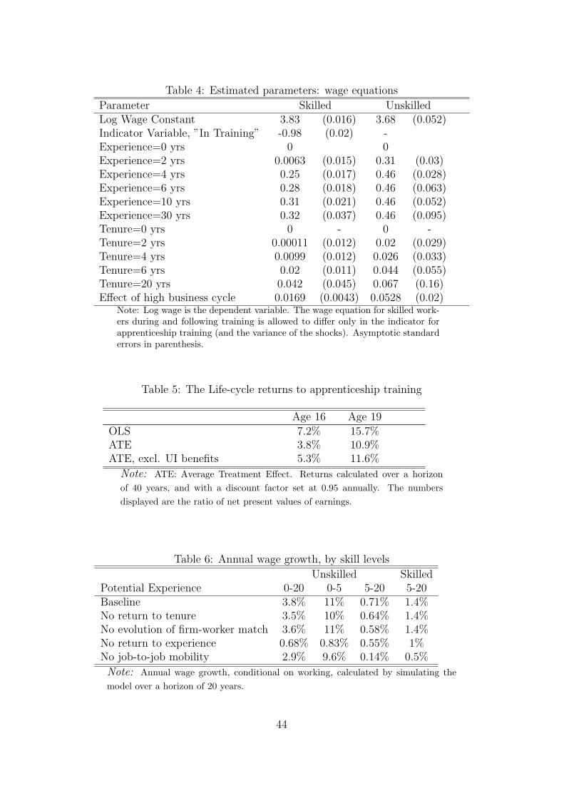
Table 4: Estimated parameters: wage equations

Parameter Skilled UnskilledLog Wage Constant 3.83 (0.016) 3.68 (0.052)Indicator Variable, ”In Training” -0.98 (0.02) -Experience=0 yrs 0 0Experience=2 yrs 0.0063 (0.015) 0.31 (0.03)Experience=4 yrs 0.25 (0.017) 0.46 (0.028)Experience=6 yrs 0.28 (0.018) 0.46 (0.063)Experience=10 yrs 0.31 (0.021) 0.46 (0.052)Experience=30 yrs 0.32 (0.037) 0.46 (0.095)Tenure=0 yrs 0 - 0 -Tenure=2 yrs 0.00011 (0.012) 0.02 (0.029)Tenure=4 yrs 0.0099 (0.012) 0.026 (0.033)Tenure=6 yrs 0.02 (0.011) 0.044 (0.055)Tenure=20 yrs 0.042 (0.045) 0.067 (0.16)Effect of high business cycle 0.0169 (0.0043) 0.0528 (0.02)

Note: Log wage is the dependent variable. The wage equation for skilled work-ers during and following training is allowed to differ only in the indicator forapprenticeship training (and the variance of the shocks). Asymptotic standarderrors in parenthesis.

Table 5: The Life-cycle returns to apprenticeship training

Age 16 Age 19

OLS 7.2% 15.7%ATE 3.8% 10.9%ATE, excl. UI benefits 5.3% 11.6%

Note: ATE: Average Treatment Effect. Returns calculated over a horizonof 40 years, and with a discount factor set at 0.95 annually. The numbersdisplayed are the ratio of net present values of earnings.

Table 6: Annual wage growth, by skill levels

Unskilled SkilledPotential Experience 0-20 0-5 5-20 5-20Baseline 3.8% 11% 0.71% 1.4%No return to tenure 3.5% 10% 0.64% 1.4%No evolution of firm-worker match 3.6% 11% 0.58% 1.4%No return to experience 0.68% 0.83% 0.55% 1%No job-to-job mobility 2.9% 9.6% 0.14% 0.5%

Note: Annual wage growth, conditional on working, calculated by simulating themodel over a horizon of 20 years.

44

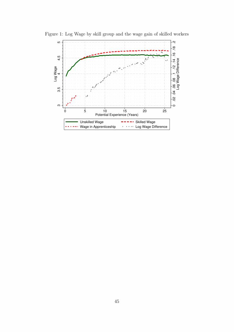
Figure 1: Log Wage by skill group and the wage gain of skilled workers

0.0

2.0

4.0

6.0

8.1

.12

.14

.16

.18

.2Log W

age D

iffe

rence

33.5

44.5

5Log W

age

0 5 10 15 20 25Potential Experience (Years)

Unskilled Wage Skilled Wage

Wage in Apprenticeship Log Wage Difference

45

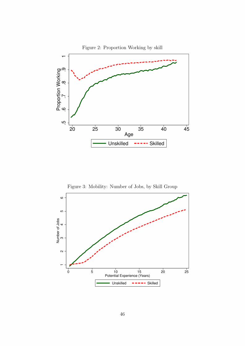
Figure 2: Proportion Working by skill

.5.6

.7.8

.91

Pro

port

ion W

ork

ing

20 25 30 35 40 45Age

Unskilled Skilled

Figure 3: Mobility: Number of Jobs, by Skill Group

12

34

56

Num

ber

of Jobs

0 5 10 15 20 25Potential Experience (Years)

Unskilled Skilled

46

Figure 4: Annual Change in Log Wage

−.0

50

.05

.1A

vera

ge C

hange in L

og W

age

0 5 10 15 20 25Potential Experience (Years)

Unskilled Skilled

Within Firms

0.1

.2.3

.4A

vera

ge C

hange in L

og W

age

0 5 10 15 20 25Potential Experience (Years)

Unskilled Skilled

Between Firms

Figure 5: Wages and Business Cycles

−500

0500

1000

1500

GD

P d

evia

tion fro

m tre

nd

−.3

−.2

−.1

0.1

Log W

age R

esid

ual

1970 1980 1990 2000 2010Year

Unskilled wage Skilled wage

GDP deviation from trend Recession

Note: GDP per capita US $, constant prices obtained from OECD. Wage dataderived from IAB sample. Residual log wages are obtained by projecting logwages on potential experience and time trend.

47

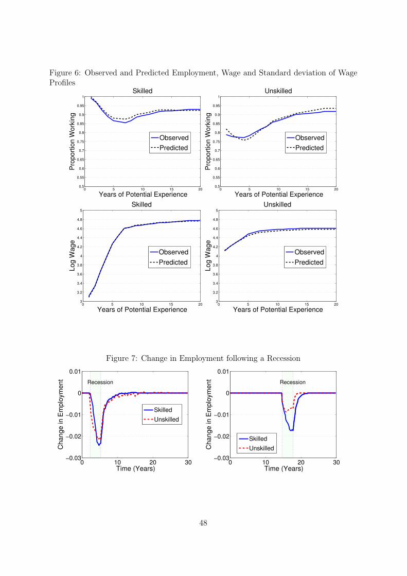
Figure 6: Observed and Predicted Employment, Wage and Standard deviation of WageProfiles

0 5 10 15 200.5

0.55

0.6

0.65

0.7

0.75

0.8

0.85

0.9

0.95

1

Skilled

Years of Potential Experience

Pro

port

ion W

ork

ing

Observed

Predicted

0 5 10 15 200.5

0.55

0.6

0.65

0.7

0.75

0.8

0.85

0.9

0.95

1

Unskilled

Years of Potential Experience

Pro

port

ion W

ork

ing

Observed

Predicted

0 5 10 15 203

3.2

3.4

3.6

3.8

4

4.2

4.4

4.6

4.8

5

Skilled

Years of Potential Experience

Lo

g W

ag

e

Observed

Predicted

0 5 10 15 203

3.2

3.4

3.6

3.8

4

4.2

4.4

4.6

4.8

5

Unskilled

Years of Potential Experience

Lo

g W

ag

e

Observed

Predicted

Figure 7: Change in Employment following a Recession

Time (Years)

Ch

an

ge

in

Em

plo

ym

en

t

Recession

0 10 20 30−0.03

−0.02

−0.01

0

0.01

Skilled

Unskilled

Time (Years)

Ch

an

ge

in

Em

plo

ym

en

t

Recession

0 10 20 30−0.03

−0.02

−0.01

0

0.01

Skilled

Unskilled

48

Figure 8: Change in Experience following a Recession

Time (Years)

Ch

an

ge

in

Wo

rk E

xp

erie

nce

Recession

0 10 20 30−0.1

−0.08

−0.06

−0.04

−0.02

0

0.02

Skilled

Unskilled

Time (Years)

Ch

an

ge

in

Wo

rk E

xp

erie

nce

Recession

0 10 20 30−0.1

−0.08

−0.06

−0.04

−0.02

0

0.02

Skilled

Unskilled

Figure 9: Change in Firm Tenure following a Recession

Time (Years)

Ch

an

ge

in

Firm

Te

nu

re

Recession

0 10 20 30

−0.2

−0.1

0

0.1

0.2 Skilled

Unskilled

Time (Years)

Change in F

irm

Tenure

Recession

0 10 20 30

−0.2

−0.1

0

0.1

0.2 Skilled

Unskilled

Figure 10: Change in Earnings following a Recessiona

Time (Years)

Ch

an

ge

in

Lo

g E

arn

ing

s Recession

0 10 20 30

−0.1

−0.05

0

Skilled

Unskilled

Time (Years)

Ch

an

ge

in

Lo

g E

arn

ing

s Recession

0 10 20 30

−0.1

−0.05

0

Skilled

Unskilled

a Note: The figures display earnings, including zero income when not working.

49

Figure 11: Change in Composition of Workers, along Unobserved Productivity Followinga Recessiona

Time (Years)

Ch

an

ge

in

ra

tio

of

Hig

h/L

ow

Pro

du

ctivity I

nd

ivid

ua

ls W

ork

ing

Recession

0 10 20 30

1

1.02

1.04

1.06

Skilled

Unskilled

Time (Years)

Ch

an

ge

in

ra

tio

of

Hig

h/L

ow

Pro

du

ctivity I

nd

ivid

ua

ls W

ork

ing

Recession

0 10 20 30

1

1.02

1.04

1.06

Skilled

Unskilled

a Note: The figures display the difference in the ratio of high versus low productivityindividuals who are working. The comparison is between two paths, without and with arecession.

50

Appendix

A Data: Sample Used for Estimation

We select all male individuals who are born between 1960 and 1972. Thus, we make sure

that no individual is older than 15 in 1975 (the minimum age at which post-secondary

labor market entry is possible), which is the first year of our data. We consider all

years between 1975 and 2004. We exclude all individuals who live in East-Germany.

We drop individuals who work in the agricultural industry, and individuals who work

in the family businesses. We restrict our sample to those who are not older than 23

when they enter the labor market the first time, and who enter the labor market with

only a lower secondary school education, who either enroll into apprenticeship training

directly, or who enter the labor market without further training.31 32 We further exclude

individuals with multiple apprenticeships (which is about 6% of the sample), and workers

who are still in training at the end of the observation window, or who have no valid wage

spells after apprenticeship training. We also exclude individuals who had a work spell

before starting apprenticeship training, and we drop individuals with unreasonably long

apprenticeship training periods (which we set to 1600 days). We restrict our analysis to

individuals with German citizenship, as individuals with non-German citizenship may

have acquired (part of) their education abroad.

The wage information in the data is the average daily wage for the length of the

working spell. A spell is at most 365 days long if the individual does not change firm,

as firms have to report yearly on their employees. If individuals change firm during the

calendar year, or exit into unemployment, we observe the average daily wage for the

period for which the individual has been in employment. Thus, every wage we observe

belongs to one particular worker-firm spell. We compute real wages in 1995 prices.

The precise distinction between individuals who enroll in a traditional apprenticeship

31In Germany, children enter primary school at the age of about 6. Primary school takes 4 years. Afterprimary school, and at the age of 10, individuals decide whether to enter one of three secondary schoolbranches: lower secondary school (which takes another 5-6 years), intermediate secondary school (whichtakes another 6 years), and higher secondary school (which takes another 9 years). For our analysis, weconcentrate on individuals who choose lower or intermediate secondary school. These two options donot allow for direct access to university, and individuals typically enroll into apprenticeship training, orenter the labor market directly.

32As the comparison group of individuals who choose upper track secondary school, which we use toimplement our selection correction, we define all those individuals who enter the labor market eitherwith an upper secondary degree (with or without further training), and before the age of 23, or withcollege- or university education, and before the age of 32.

51

scheme (”skilled workers”), and individuals who enter the labor market without further

training (”unskilled workers”), is as follows. We define as “skilled workers” all those

individuals who entered the labor market with a lower or intermediate secondary school

degree, who can be observed after entry on an apprenticeship training scheme for at least

24 months, and who transit to a “skilled” status afterwards.33 We define as “unskilled

workers” all those individuals who enter the labor market without further training, or

who have been on an apprenticeship training schemes for less than 7 months, without

obtaining a degree (i.e. dropouts). This group may include individuals who enrolled in

one-year vocational courses before entering the labor market – preparatory courses that

do not lead to vocational degrees. Thus, among our unskilled workers may be individuals

who did receive some preparatory training.

Another mode of entry, as discussed in Parey (2009), is attendance of 2-3 year vo-

cational schools, which provide vocational training with unpaid work experience in spe-

cialized schools for a limited number of occupations. 34 These occupations are mainly

in female-dominated occupation groups, like caring and health-related occupations. In

our sample, these individuals constitute about 6% of individuals.35 In line with Parey

(2009), we find that the wage paths of this group are very similar to those of individuals

undergoing firm-based training. We thus include them in the group of skilled workers, as-

suming that the choice to undergo training at a full time school is equivalent to choosing

apprenticeship training in a firm.

B Model and Numerical Solution

B.1 The value of unemployment.

The value of unemployment consists of a predetermined part and a stochastic shock ηit

reflecting changes in the utility of being out of work. Denoting the predetermined part

by Ua(Si, Gt, Xit, wi(−1), εi

), where the subscript a denotes the age of the individual, we

33For apprentices who finish their training within a calendar without changing firms, we do not observethe date of graduation, neither can we distinguish the apprenticeship wage during that year from theskilled worker wage. To compute the number of apprenticeship training months, we assign to theseindividual 6 months of training. Further, when we compute wages after the apprenticeship period, wediscard these observations.

34According to the Central Labor Office (Bundesagentur fuer Arbeit), firm based apprenticeshipschemes train for 541 occupations, while full-time colleges train for only 133 occupations.

35The size of this group is smaller than in Parey (2009). One reason for this is that we consider onlythe years up to 1996, where these school based vocational schemes were less frequent than in later years.

52

can write

Ua(Si, Gt, Xit, wi(−1), εi

)= log(γUwi(−1)) + γ(Xit, Si, εi) A

+βπUit E max

µi +Wa+1

(Si, Gt+1, Xit, Tit+1 = 0, κi0, εi

)Ua+1

(Si, Gt+1, Xit, wi(−1), εi

)+ ηit+1

B

+β(1− πUit ) EUa+1

(Si, Gt+1, Xit, wi(−1), εi

)C

(B1)

where we underline the variables over which we are taking expectations (because they

are unknown to the individual in period t) and where β is the discount factor.

In (B1) the first line of the right hand side (A) represents the within period value of

being out of work (up to the stochastic shock ηit). This consists of the unemployment

insurance income plus a value for leisure. The lines denoted by (B) represent the expected

future value for the case where the worker gets a job offer, which happens with probability

πUit . In that case the worker will choose the best of taking the job offer or continuing

as an unemployed worker. The value of taking the job offer is equal to the sum of the

present value of the future flow of earnings defined below, Wa+1(·), plus a (stochastic)

amenity µi. The final line (C) represents the case where the individual obtains no offer

and thus just has to continue out of work.

B.2 The value of employment.

Their value of employment is then given by:

Wa (Si, Gt, Xit, Tit, κit, εi) = log(wit) A

+βδit E[Ua+1

(Si, Gt+1, Xit + 1, wit

)+ ηit+1

]B

+β (1− δit) πWit E max

Ua+1

(Si, Gt+1, Xit + 1, wit, εi

)+ ηit+1

Wa+1

(Si, Gt+1, Xit + 1, Tit + 1, κit + uit+1, εi

)µi +Wa+1

(Si, Gt+1, Xit + 1, Tit+1 = 0, κi0, εi

) C

+β(1− δit)(1− πWit ) E max

Ua+1

(Si, Gt+1, Xit + 1, wit, εi

)+ ηit+1

Wa+1

(Si, Gt+1, Xit + 1, Tit + 1, κit + uit+1, εi

) D

(B2)

The current value of work is just the wages wit. Following job destruction, which occurs

with probability δit the individual will receive the value of unemployment as shown in line

53

B. The group of lines marked C represent the events when the job is not destroyed and

the individual obtains an alternative job offer. In this case they have to choose between

becoming unemployed; remaining with the firm; or taking the alternative offer, which is

associated with the one off random switching cost µi of joining a new firm. The following

group of lines marked by D represent the expected value of a worker not being laid off

and not having access to an alternative offer. Given that a shock can occur to the match

specific effect, the worker may decide it is best to quit, in which case they receive the

value of unemployment. Otherwise they receive the value of working with the same firm,

at the updated wage.

B.3 The value of employment while in training.

Going back, earlier into the individual’s history, we consider choices available when

training. During apprenticeship (which lasts τA periods36) we assume that the train-

ing firm pays the worker only a fraction λA of his productivity as an unskilled worker

(w (Si = 0, Gt, Xit, Tit, κit, εi)), the reminder serving as payment for the general training

received. Reflecting the facts in the data, we do not allow the individual to experience

unemployment during apprenticeship, although they can decide to change firm if the

opportunity arises. Thus, during the apprenticeship training period (Xit < τA) the value

of work is:

WAa (Gt, Xit, Tit, κit, εi) = log(λA · w (Si = 0, Gt, Xit, Tit, κit, εi)) A

+βπA(Gt) E max

(WAa+1

(Gt+1, Xit + 1, Tit + 1, κit + uit+1, εi

)µi +WA

a+1

(Gt+1, Xit+1, Tit+1 = 0, κi0, εi

) )B

+β[1− πA(Gt)] EWAa+1

(Gt+1, Xit + 1, Tit+1, κit + uit+1, εi

)C

(B3)

where as before, the expectation operator E relates to the underlined variables, which

are unknown to the individual in period t.

Similarly to the value of working described above, the first line (A) is earnings while

training, (B) represents the part of the value due to the possibility of changing training

firms if an offer arrives (with probability πA). As before there is a mobility cost associated

with the decision to join the alternative firm. Finally, line (C) represents the continuation

value for the case where no alternative training firm is available. While in the last

36Apprenticeship courses last between two and three years. We equate τA to whatever is the actualduration in the data.

54

period of apprenticeship the value function becomes as in equation (B2) with all options

available.

B.4 The time horizon and the terminal condition

We solve for the value functions at each age by backwards induction from retirement,

which occurs at 65 years of age, to the start of the labor market career when the ap-

prenticeship choice is made at 16. At retirement the value is assigned to zero: in a

linear utility framework, such as ours, this is equivalent to assuming that individuals

finance retirement through their own savings out of their wages.37 Having a terminal

point beyond our observation window requires assumptions on the returns to experience

and tenure. Noting from the data that there is almost no wage growth beyond 11 years of

potential experience we imposed that the returns to experience and tenure are constant

between 10 and 30 years of actual experience.38 We then assume that there is no wage

growth beyond 30 years of experience and tenure respectively. The gain from this tight

specification is that we avoid having to use a separately parameterized terminal value

function. Further computational details can be found in Appendix C.

C Computational Details

C.1 GDP growth and Markov transition matrix

To compute business cycles, we use the per capita West-German GDP expressed in

constant prices, obtained from the OECD for the period 1975-2009. We linearly detrend

the series and use transitions between above trend (good times) and below trend (bad

times). Table A1 presents the transition matrix for this first order Markov process,

estimated over our sample period.

C.2 Computing the Value Functions

The model is solved recursively backward, starting at age 65 and until age 16. We allow

the value function to depend on age as well as the other state variables.

We integrated out analytically as many state variables as possible (shocks to the value

of leisure (η), shocks to the cost of training ω, and shocks to cost of moving µ ). We

approximate the value functions by evaluating them at a number of discrete points in the

37Note that the model uses gross wages, before any pension contributions.38Thus, extrapolating from our data which stops at 30 years of experience

55

state space and interpolating linearly in between. For experience and tenure the points

where we evaluate are 0, 2, 4, 6, 10 and 30 years of experience and 0, 2, 4, 6 and 30

years of tenure; this level of detail turned out to be sufficient. The other state variable

is the firm-worker match specific effect which evolves as a random walk while the worker

remains in the same job. We use 10 points on a grid which depends on skills and on

tenure to take into account the non-stationary nature of the process. More specifically,

given the assumptions made, the match effect is a normal variable with mean zero and

variance TσU(Skill)2 + σ0(Skill)2 for an individual with T years of tenure. We use a

quadrature-based method as in the Tauchen and Hussey (1991) procedure to generate a

grid and transition matrices. We interpolate between the points.

The code was solved using parallel processing to increase speed.

D The Fit of the Model

In this section, we present the fit of the model in detail in Tables A3 to A12. The tables

list all the moments used in the estimation, apart from the ones used to identify the

educational choices at age 10 and 16, as they involve more than 100 entries each and are

too long to display.

E Additional Parameters

In Table A2 we display the parameters of the model which are associated with unobserved

heterogeneity. We model these two types of ability as a bivariate mass-point distribution

with two points of support, and allow for the possibility that the two dimensions of

unobserved heterogeneity are correlated. This results in four groups: individuals with

high ability (which we denote ”Type 3” and ”Type 4”) and individuals with high costs

of training (”Type 2” and ”Type 4”). As shown in Table A2, high ability individuals

and those with lower cost of education are more likely to become skilled workers. This

is because the returns to choosing a skilled career is higher.

56

Table A1: Quarterly transition matrix for below and above trend GDP

Below Trend in t+1 Above Trend in t+1Below Trend in t 0.9302 (0.039) 0.069 (0.039)Above Trend in t 0.075 (0.042) 0.925 (0.042)Note: Note: Data source: OECD, GDP per capita, constant prices,constant PPP, period 1975-2009. Asymptotic standard errors in paren-thesis.

Table A2: Estimated parameters: unobserved heterogeneity

Parameter Type 1 Type 2 Type 3 Type 4Proportion in sample (πj) 0.21 0.2 0.21 0.38Proportion skilled 0.98 0.83 0.99 0.87Log wage constant, skilled worker(α0(ε)) 0 0 0.35 0.35

(0.023) (0.023)Log wage constant, unskilled worker (α0(ε)) 0 0 0.55 0.55

(0.33) (0.33)Utility gain of training (−λ0(ε)) 483 0 483 0

(0.0228) (0.0228)Correlation between types -0.15

Note: a: as a percentage of the value of leisure for skilled workers. b: as apercentage of lifetime value. Asymptotic standard errors in parenthesis.

Table A3: Goodness of Fit: Wage Level and Potential Experience

Apprentices Non ApprenticesObserved Std Error Simulated Observed Std Error Simulated

Potential Exp ∈ [0,2] 3.09 (0.002) 3.07 4.09 ( 0.01) 4.12Potential Exp ∈ ]2,4] 3.78 (0.003) 3.78 4.37 (0.009) 4.37Potential Exp ∈ ]4,6] 4.52 (0.002) 4.52 4.5 (0.007) 4.5Potential Exp ∈ ]6,8] 4.62 (0.002) 4.64 4.55 (0.008) 4.54Potential Exp ∈ ]8,10] 4.71 (0.003) 4.71 4.58 ( 0.01) 4.59Potential Exp ∈ ]10,15] 4.75 (0.004) 4.74 4.59 ( 0.01) 4.61Potential Exp ∈ ]15,30] 4.78 (0.005) 4.75 4.58 ( 0.02) 4.61Business Cycle Good 0.0336 (0.002) 0.0315 0.046 (0.009) 0.0459Business Cycle Good, Pot. Exp>4 0.00819 (0.002) 0.0112 -0.0106 (0.009) 0.0148

57

Table A4: Goodness of Fit: Proportion Working and Potential Experience

Apprentices Non ApprenticesObserved Std Error Simulated Observed Std Error Simulated

Potential Exp ∈ [0,2] 0.984 (0.001) 0.995 0.76 (0.007) 0.792Potential Exp ∈ ]2,4] 0.907 (0.001) 0.903 0.751 (0.008) 0.719Potential Exp ∈ ]4,6] 0.815 (0.002) 0.842 0.786 (0.008) 0.761Potential Exp ∈ ]6,10] 0.876 (0.002) 0.889 0.847 (0.008) 0.85Potential Exp ∈ ]10,15] 0.915 (0.002) 0.923 0.901 ( 0.01) 0.9Potential Exp ∈ ]15,20] 0.926 (0.003) 0.92 0.918 ( 0.01) 0.934Potential Exp ∈ ]20,40] 0.935 (0.003) 0.921 0.952 ( 0.01) 0.941Business Cycle Good 0.0188 (0.001) 0.011 0.061 (0.007) 0.0545Business Cycle Good, Pot. Exp>4 -0.014 (0.001) -0.00349 -0.0633 (0.007) -0.0489

Table A5: Goodness of Fit: Experience Levels and Potential Experience

Apprentices Non ApprenticesObserved Std Error Simulated Observed Std Error Simulated

Potential Exp ∈ [0,2] 0.942 (0.01) 0.875 0.765 (0.05) 0.779Potential Exp ∈ ]2,4] 2.68 (0.01) 2.82 2.19 (0.05) 2.31Potential Exp ∈ ]4,6] 3.98 (0.01) 4.56 3.6 (0.06) 3.85Potential Exp ∈ ]6,10] 6.07 (0.01) 7.15 5.88 (0.07) 6.31Potential Exp ∈ ]10,15] 9.73 (0.02) 11.3 9.63 (0.09) 10.2Potential Exp ∈ ]15,20] 14 (0.03) 15.9 14 ( 0.1) 14.9Potential Exp ∈ ]20,40] 18.8 (0.04) 21.2 19.1 ( 0.2) 20.3

Table A6: Goodness of Fit: Firm Seniority and Potential Experience

Apprentices Non ApprenticesObserved Std Error Simulated Observed Std Error Simulated

Potential Exp ∈ [0,2] 0.845 ( 0.03) 0.872 0.866 (0.08) 0.832Potential Exp ∈ ]2,4] 2.27 ( 0.03) 2.35 2 (0.09) 1.97Potential Exp ∈ ]4,6] 2.67 ( 0.03) 2.6 2.8 (0.09) 2.6Potential Exp ∈ ]6,10] 3.48 ( 0.03) 3.18 4.03 ( 0.1) 3.44Potential Exp ∈ ]10,15] 5.09 ( 0.05) 4.77 5.84 ( 0.1) 4.77Potential Exp ∈ ]15,20] 7 ( 0.06) 6.22 7.85 ( 0.2) 5.37Potential Exp ∈ ]20,40] 8.92 ( 0.09) 7.4 9.74 ( 0.3) 5.74Business Cycle Good -0.0111 (0.006) -0.0518 -0.0813 (0.03) -0.135Business Cycle Good, Pot. Exp>4 0.0814 ( 0.02) 0.0833 0.0905 (0.06) 0.17

58

Table A7: Goodness of Fit: Number of Firms and Potential Experience

Apprentices Non ApprenticesObserved Std Error Simulated Observed Std Error Simulated

Potential Exp ∈ [0,2] 1 ( 0.01) 1.04 0.91 (0.06) 1.13Potential Exp ∈ ]2,4] 1.13 ( 0.01) 1.27 1.56 (0.06) 1.46Potential Exp ∈ ]4,6] 1.56 ( 0.01) 1.74 2.14 (0.06) 1.83Potential Exp ∈ ]6,10] 2.32 ( 0.02) 2.41 2.89 (0.08) 2.38Potential Exp ∈ ]10,15] 3.2 ( 0.02) 3.15 3.86 ( 0.1) 3.02Potential Exp ∈ ]15,20] 3.91 ( 0.03) 3.84 4.67 ( 0.1) 3.74Potential Exp ∈ ]20,40] 4.62 ( 0.05) 4.62 5.5 ( 0.2) 4.55Business Cycle Good 0.00241 (0.004) -0.00789 0.101 (0.02) -0.0573Business Cycle Good, Pot. Exp>4 0.0362 (0.007) 0.0387 -0.0296 (0.03) 0.0472

Table A8: Goodness of Fit: Standard Deviations of Wages and Potential Experience

Apprentices Non ApprenticesObserved Std Error Simulated Observed Std Error Simulated

Potential Exp ∈ [0,2] 0.337 (0.004) 0.339 0.489 ( 0.01) 0.381Potential Exp ∈ ]2,4] 0.485 ( 0.03) 0.501 0.4 (0.009) 0.395Potential Exp ∈ ]4,6] 0.312 (0.007) 0.332 0.353 (0.004) 0.402Potential Exp ∈ ]6,10] 0.301 (0.002) 0.288 0.35 (0.002) 0.399Potential Exp ∈ ]10,15] 0.334 (0.002) 0.272 0.377 (0.001) 0.383Potential Exp ∈ ]15,40] 0.31 (0.002) 0.276 0.323 (0.005) 0.387

59

Table A9: Goodness of Fit: Wages, Experience and Tenure

Apprentices Non ApprenticesObserved Std Error Simulated Observed Std Error Simulated

Exp ∈ ]2,4] 0.221 ( 0.002) 0.163 0.256 (0.006) 0.25Exp ∈ ]4,6] 0.437 ( 0.003) 0.434 0.339 (0.009) 0.346Exp ∈ ]6,8] 0.509 ( 0.003) 0.504 0.365 ( 0.01) 0.359Exp ∈ ]8,10] 0.552 ( 0.004) 0.542 0.384 ( 0.01) 0.375Exp ∈ ]10,15] 0.594 ( 0.004) 0.56 0.397 ( 0.01) 0.407Exp ∈ ]15,40] 0.647 ( 0.005) 0.573 0.414 ( 0.02) 0.405Tenure ∈ ]2,4] 0.00417 (0.0009) 0.043 0.0418 (0.004) 0.0369Tenure ∈ ]4,6] 0.0326 ( 0.001) 0.0855 0.0704 (0.005) 0.047Tenure ∈ ]6,8] 0.039 ( 0.002) 0.118 0.0778 (0.007) 0.057Tenure ∈ ]8,10] 0.0473 ( 0.002) 0.137 0.0841 (0.008) 0.0802Tenure ∈ ]10,40] 0.065 ( 0.003) 0.171 0.0817 ( 0.01) 0.0752Business Cycle Good 0.0293 ( 0.002) 0.0355 0.0432 (0.009) 0.0343Business Cycle Good, Pot. Exp>4 0.0129 ( 0.002) 0.00668 -0.0053 (0.009) 0.0264In Apprenticeship Training -1.01 (0.003) -0.994 - - -Constant 4.12 (0.003) -0.994 4.15 (0.009) 0.0264

Table A10: Goodness of Fit: Standard Deviation of Wages, Experience and Tenure

Apprentices Non ApprenticesObserved Std Error Simulated Observed Std Error Simulated

Exp -0.0024 (0.0003) -0.00404 -0.02 (0.001) -0.000495Exp squared 0.000123 ( 1e-05) 0.000116 0.000689 (5e-05) 4.27e-05Tenure -0.00332 (0.0002) -0.00495 -0.00683 (0.001) -0.00257Tenure squared 9.49e-05 ( 1e-05) 0.00016 0.000278 (5e-05) 6.61e-05Business Cycle Good 0.0156 ( 0.001) 0.0211 0.0184 (0.007) 0.00732Business Cycle Good, Pot. Exp>4 -0.0306 ( 0.001) -0.0298 -0.0144 (0.007) -0.00574In Apprenticeship Training 0.00503 (0.001) 0.0214 - - -Constant 0.0963 (0.001) 0.126 0.215 (0.006) 0.154

60

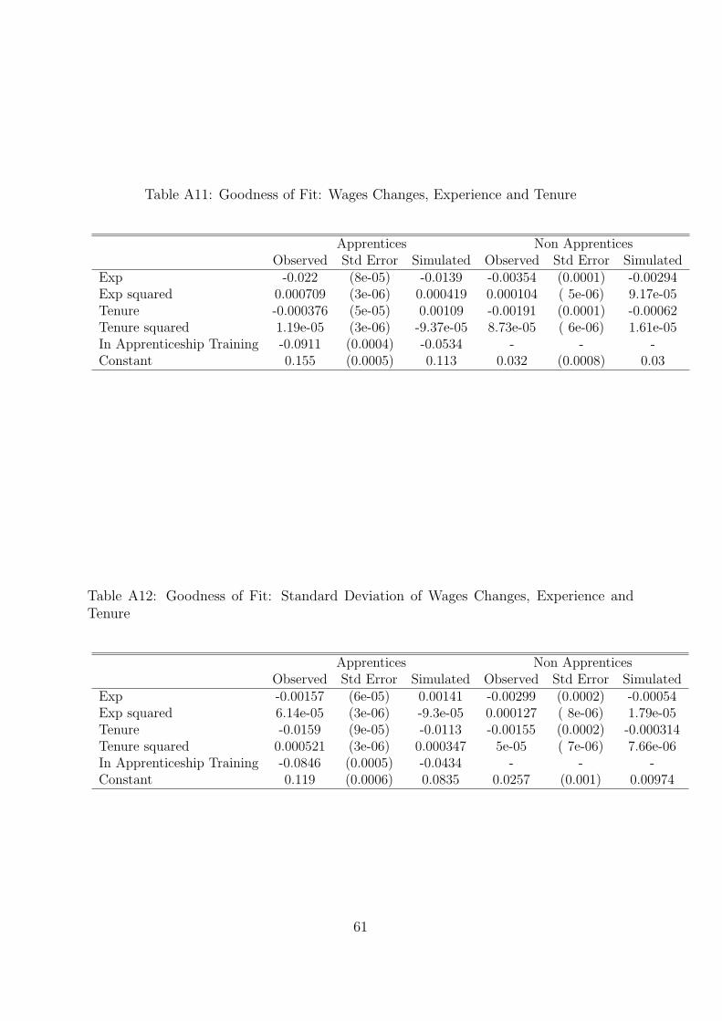
Table A11: Goodness of Fit: Wages Changes, Experience and Tenure

Apprentices Non ApprenticesObserved Std Error Simulated Observed Std Error Simulated

Exp -0.022 (8e-05) -0.0139 -0.00354 (0.0001) -0.00294Exp squared 0.000709 (3e-06) 0.000419 0.000104 ( 5e-06) 9.17e-05Tenure -0.000376 (5e-05) 0.00109 -0.00191 (0.0001) -0.00062Tenure squared 1.19e-05 (3e-06) -9.37e-05 8.73e-05 ( 6e-06) 1.61e-05In Apprenticeship Training -0.0911 (0.0004) -0.0534 - - -Constant 0.155 (0.0005) 0.113 0.032 (0.0008) 0.03

Table A12: Goodness of Fit: Standard Deviation of Wages Changes, Experience andTenure

Apprentices Non ApprenticesObserved Std Error Simulated Observed Std Error Simulated

Exp -0.00157 (6e-05) 0.00141 -0.00299 (0.0002) -0.00054Exp squared 6.14e-05 (3e-06) -9.3e-05 0.000127 ( 8e-06) 1.79e-05Tenure -0.0159 (9e-05) -0.0113 -0.00155 (0.0002) -0.000314Tenure squared 0.000521 (3e-06) 0.000347 5e-05 ( 7e-06) 7.66e-06In Apprenticeship Training -0.0846 (0.0005) -0.0434 - - -Constant 0.119 (0.0006) 0.0835 0.0257 (0.001) 0.00974

61