-------------------------------------------

----------------------------

------------------------

Working Paper 98-21 Departamento de Estadística y Econometría

Statistics and Econometrics Series 14 Universidad Carlos III de Madrid

February 1998 Calle Madrid, 126

28903 Getafe (Spain)

Fax (341) 624-9849

LOCAL CROSS VALlDATION FOR SPECTRUM BANDWIDTH CHOICE.

Carlos Velasco*

Abstract

We investigate an automatic method of determining a local bandwidth for nonparametric

kernel spectral density estimates at a single frequency. This procedure is a modification of

a cross-validation tecnique for global bandwidth choices, avoiding the computation of any

pilot estimate based on initial bandwidths or on approximate parametric models. Only

local conditions on the spectral density around the frequency of interest are assumed. We

illustrate with a Monte CarIo study the performance in finite samples of the bandwidth

estimates proposed.

Keywords:

Bandwidth selection, nonparametric spectral estimation, cross-validation, time series,

periodogram.

*Departamento de Estadística y Econometría, Universidad Carlos nI de Madrid. CI

Madrid, 126 28903 Madrid. Spain. Ph: 34-1-624.98.87, Fax: 34-1-624.98.49, e­

mail: cavelas@est-econ.uc3m.es.This paper is a revised version of the Chapter 4 of

the author's University of London Ph.D. Thesis. I am grateful to Professor P.M.

Robinson for his guidance and advice. Research funded by the Spanish Dirección

General de Enseñanza Superior, Ref. n. PB95-0292.

Local Cross Validation for Spectrum Bandwidth Choice

Carlos Velasco

Departamento de Estadística y Econometría

Universidad Carlos Ilr de Madrid

Calle Madrid 126

28903 Getafe (Madrid)

Spain

1

1

Local Cross Validation for 8pectrum Bandwidth Choice

Carlos Velasco*�

Departamento de Estadística y Econometría�

Universidad Carlos IU de Madrid�

Calle Madrid 126�

28903 Getafe (NIadrid)�

Spain�

February 2, 1998

Abstract

\rc investigate an automatic rnethod of determining a local bandwidth fOl' nonpararnetric

kcmd spectral clensity estimates at a single frequency. Tltis procecdure is a 1l10dification of

a ('J'oss-validation technique for global banclwiclth choices, avoiding the computation of any

pilot estimate based on initial bandwidths 01' on approximate parametric models. Only local

cOllditions on the spectral clensity around the frequency of interest are assumecl. \Ve illus­

1rate' with a Monte Cario study the performance in finite samples of the bandwiclth cstimates

proposed.

I\:eywords. Dancl\viclth sclection; 1l0l1paramctric slwct.rill l'stimation; c:ross-validation;

1ittt<, series; perioc1ogram.

Introduction

Smootlwd estimation of the spectral density of stationary time series, like many nonparametric

methods uf infel'ence, relies on the choice of a bandwidth 01' lag numbel' depending on the sample

size. Thc properties of the estimates depend cl'ucial1y on the value of this number. Asymptotic

theory l)l'(~scl'ibes arate fol' the lag numbel' M with l'espect to the sample size N as this tends to

infinity, but gives no pl'actical guidance fol' the choice of M in finite samples. Different techniques

have hocn proposed in the litel'atUl'e to that end. The usual cl'itel'ion is the minimization of sorne

'This p¡\per is a revised version of the Chapter 4 of the author's University of London PhD Thesis. 1 am

grateful to Professor P.M. Robinson for his guidance and advice.

2

estimate of the asymptotic mean square error of the estimator. This can be illlplemented by

plug-in or cross-validation methods. Also, global and local choices are possible, depending on

whether we are interested in the behaviour of the spectral density for all range of frequencies or

in a specific point or small interval.

Tbe plug-in method consists in substituting the unknowns of tbe leading term in tbe asymp­

totic expression for the mean square error by consistent estimates, generally nonparametric, but

also parametric ones based on approximate models can be used. Cross validation procedures

avoid the use of those initial estimates and approximate the mean square error illdirectly. They

are based on estimates which do not use the information contained in the sample about the

function of interest at each point (at each Fourier frequency in the case of spectral estimation).

Wahba (Hl8ü) considered automatic smoothing methods fOl' tbe log periodogram, but in many

cases w(~ are interested in obtaining optimal bandwidths for the original scale.

Bcltrao and Bloomfield (1987) (BB hereafter) considered bandwidth choice for discrete pe­

riodogram average type spectral estimates. Thcy justificd a lllethod based on (1 cross-validated

form of vVhittle's frequency domain approximation to the likelihood function of a stationary

GauSSi(111 process (see also Hurviclr (1985)). Robinson (1991) extended their results under more

generaJ conditions for a wider class of models, including spectral estimation for the construction

of efficient regression estimates, and proved the consistency of the estimate of A1. This cross­

validatcd lllethod selects a global bandwidth for a11 the range of frcquencies [-7f, 7f] 01' for a fixee!

subset of it. Here we propose a modified version of crOS8 validation to jU8tify a local bandwie!tb

cllOic(~ fOl' a single frequency, following sorne ideas suggestcd in Robinson (1991, p. 1346), relatee!

with the work of Hurvicb and Beltrao (1994) in a different contexto For tbis single frequency

choic(~. W(' only use local smootlmess properties of the spectral density of the time series aroune!

this frequency, allowing for a broader range of dependence models. This local ae!aptation could

leae! al80 to efficiency gains when estimation of the spectnllll for aH range of frequencies [-7f, 7f]

is in lllind.

The lllethod we analyze here can be seen as the cross validation alternative to Bühlmann's

(1996) iterative local plug-in procedure for lag-window spectral estimates, proposed by Brock­

mann et al. (1993) in the context of kernel regression estimators (see also Herrmann (1997)), or

to the related proposal of Newey and West (1994) for covariance matrix estimatioll. Local adap­

tatioll is a180 studied by Lepskii and 8pokoiny (1995) for projective estimates in a "signal+noise"

model. Here the range of estimation is split on degenerating intervals with the asymptotics and

different smoothing parameters are estimated independently for each one.

Next section is devoted to the assumptions that we wil! use in this papel', together with a

3

2

brief introduction to the main cross validation concepts for nonparametric spectrum estimation

and a detailed analysis of the mean square error for the spectral estimate at a fixed frequency

under local smoothness assumptions. Section 3 introduces the local cross validation criterion

and the main result of the paper. Then we carry out a Monte Carlo analysis of the finite sample

behaviour of the techniques proposed. AH the proofs and sorne technical lemmas required are

given in the Appendix.

Assumptions and definitions

In this section we will introduce sorne assumptions and definitions, together with sorne intuitions

abollt c:ross validation and BB's results. Given the observed data Xt, t = 1,2, ... , N, the

periodogram at the frequency Aj = 27fj / N, j integer, is equal to

The <t\'('raged-periodogram spectral estimate with lag llumber 1\;/ = MN = h¡/, where hN is tlw

balldwidth of the estimate in BB's notation, and kemel or spectral window K (this function was

denoted by W in BB, but we use this notation later for another analogous funchon), is

fM(Aj) (~ o~/ L K(M Ad I(Aj - Ak), k

where the snmmation runs for aH values of k in tho support of K (llot inclucling aH the peri­

oc1ogrilln ordillates equal to the zero frequency periodogralll to aCC:Ollnt for mean c:orrection).

and al! gi\'es the exact sum of the weights used

Bere \\.(~ could have used the value 27f M/N instead of o¡:/ , using that K integratcs to 1, but this

simplifies some arguments. We stress the dependence of f/ll on M in the notation, sinc:e tllis is

the ¡J(J,1'(J,rncter of interest.

DD (d. their Theorem 3.1) considered a zero mean statiollary Gaussiall process {Xd with

autoco\'ariance function ,(r) = E [XoXrJ satisfying

00

L rli(r)1 < 00,

1

alld spectral density f(A) = (27f)-1 ¿~oo ,(r) exp{irA} everywhere positive. The kernel function

K tite,)' used for the nonparametric estimates was non-negative, even, bounded function, with

2i: K(x)dx = 1, i: x K(x)dx < oo.

4

Also we can write K(x) = Jw(y) exp{ixy}dy, where w is of compact support. The bandwidth

hN satisfies h¡/ = O(NP), for some p < ~ and hN = 0(1).

The 'leave-two-out version' of the estimator 1M (we leave only two frequencies out if K were

actually compactly supported inside [-1T, 1T], as we will assume later on, or if we had defined its

periodic version in that interval) is

~ j ( ) de! -1 ",' (f M Aj = O'j,M L.J K MAk) I(Aj - Ak), (1) k

where ¿h:' runs for the same values as before, except in the set of indices of frequencies Aj - AA:

with the same periodogram ordinate as I(Aj), i.e., k E {a, ±N, . .. } U {2j, 2j ± N, . .. }. Also, the

normalizing number O'j,M is now equal to

de! ",'O'j,M = L.J K(MAA;).

k

Intl'odueo the pseudo log-likelihood type criteriOll

N-1

L(f) (~ ¿ {log f(Aj) + I(Aj)/f(Aj)} , (2) j=l

which is Whittle's approximation for the likclihood of a Gaussian sequ€nce in the fl'equency

dornain. 13B showcd undel' thc previous eonditions that

L (1/1'[) - L(f) = ~ IMSE(M)

plus a b~l'm of srnaller order in probability, where IMSE(M) is thc discrete approximation to the

Illtegratec! Mean Squarcd Error of hu, weighted by f-1:

N-1

IMSE(M) (~ N- 1 ¿ E [{ 1M(Aj) - f(Aj)} / f(Aj)r. j=l

Thcll millilllizillg L (11\'[) and IMSE( M) should be appl'oxirnately equivalellt, aud this is tho

basis for the estimation of the M that minimizes IMSE(M) for 1M(A) in [-1T,1T].

If we are interested in nonparametric spectral estimation at a single frequency (of special

intel'cst is the zero one; see Bühlmann's (1996) examples, together with covariance matrix es­

timatiou in econometrics, like in den Haan and Levin (1996) and the references therein) or we

want to achieve possible efficiency gains using different bandwidths for eaeh frequency, we need

a cl'itcriou to choose a local bandwidth. The Mean Square Error at a frequency //,

de! [{ ~ }]2MSE(IJ, M) = E fM(V) - f(v) / f(v) ,

is the usual criterion employed to assess nonparametric estimates of this class at a single fre­

queucy. We consider only fixed frequencies of the form v = 21TV/N, where v is an integer. We

restrict t,o a ::; v ::; ~ N, given the symmetry and periodicity of the periodogram alld the spectral

density. We will use the following Assumptions:

5

Assumption 1 X t , t = 1,2, ... is a Gaussian stationary time series.

Assumption 2 The spectml density f(A) of X t has thrce uniformly bounded der'ivatives in an

interval a7'Ound the fixed frequency v, with f(A) > Ofor A in that interval, and f E L p [-7f, 7fJ for

5some p > }.

Assumption 3 The function K is non-negative, even, bounded, zero outside [-7f, 7f], of bounded

variation and

f'OOi: K(x)dx = 1, x 2K(x)dx = W2 < oo. -00

Assumption 4 The function K has Fourier tmnsforrn W(.7;) = (27f)-1 J~oo K(A)ci>'xdA satisfy­

mg

for 80lne (Y > i.

ASSlllnptioll 1 was used also in BB, but we do not nacd to assume zero mean since we avoid

thc zero frcquency periodogram ordinate in the definitioll of our estimates. Asslllnption 2 only

requires smootlmess properties of f around tlw frequcnc:y we are interested in, allowing for a

wide class of spec:tral densities, including ones with zaros ami poles outside a ncighbourhood

of u. Tlw only requirement outside this band is an intcgrability condition to ensure ergoclicity

(with n~sIJect to second llloments) of the series (see Lemma 7 below).

A compac:t support kernel in Assumption 3 is then the c:omplementary of ASSulllption 2 in

order to ¡.';l1arantee that we only use information in an interval around u. The n~st of conditions

on I{ <Ire standard, Assumption 4 being necessary to approximate frvr with a weighted autoco­

variallC(' type est.imate in Lemma 5. From this lomma. bot.h ostimatos have the samo asymptotic:

c1istribution and mean square error, so the bandwidth choice techniques for one are valid for the

othcr. This condition is satisfied by the Barlett-Priestley and quadratic spectral ker'nels (with

a = 2), but not by the Daniell or uniform spectral window.

With Assumption 3, the summation in k in the definition of .1111 takes valucs in {j - N + 1, ... ,j -1} - {j} due to the compact support kernel, and in {j - N +1, ... ,j -1} - {j, 2j, 2j - N}

for .tf\jr (Al) .

\Ve llOW present a result concerning the mean square error of the estimate .tM at Fourier

freql1enc:i(~s, which will be used to analyze a local version of the likelihood (2). We use in tho

proof t.wo lemmas given in the Appendix about the discrete Fourier transform amI periodogram

of tllP observed sequence, extending and correcting sorne of the results of BB, assuming only

local smoothness for the spectral density. We have to distinguish between estimates for Fourier

6

3

frequencies Aj close to the origin, and at remote frequencies. Define IIKII~ = JK 2(x)dx and c a

finite positive constant, not necessarily always the same.

Lemma 1 Under Assumptions 1, 2 and 3, if M = e· N i / 5 , for frequeneies Aj = 27fj/N sueh

ithat Iv - Aj! ::; e· m- for some positive sequenee m sueh that l/m +m/M -+ 0, then, uniformly

in j, for 1/ > 0,

(3)

and for 1/ = 0,

when~ °::; O!vI (j) ::; 1 measures the degree of ovedapping úetween different kernels J( at a distant

2MAj apart when Aj -+ O as N -+ oo. For j = 0, OM(j) = 1 VM, andfor Aj > 27f/M, O!vI(j) = O.

Fol' 1/ > °this is the standard result 1'01' globally smooth spectral densities (see 1'01' example

Brillinger (1975), Corollaries 5.6.1 and 5.6.2). However in a degenerating band around the origin

(small Aj), the nonparametric spectral estimates llave variance depending on the overlapping 01'

two kernel functions J( centl'ed at fl'equcncics Aj and -A) l'espcctively, measured by the quantity

To malee thc bias ano the Val'iallCC 01' the same ol'del' 01' lllagllitudc we would tale M = T Ni/.s,

1'01' SOllW () < T < oc: alld then MSE will be 01' arcler 1\1-"1 '" cM/ N. From the pl'cvious lemllla,

thc optilllal COllstallt T* that minimizes the leading tenll 01' MSE 01' h¡¡(v) is

(5)

if 1/ 1- Oalld with 47f instead 01' 27f 1'01' v = O. Now it is possible to estimate the value 01' T* using

initiaL pilot estimates 01' the spectral density and its secono dcrivative at v. This is the approach

01' several authors, including Andrews (1991), Newey and West (1994) or Bühlmann (1996), just

to givc SOllle recent contributions. In the following section we adopt instead an indirect approach

using a cross-validation argumento

Local cross validation

Consicler 1'01' some positive sequence m = mN such that m- 1 + m/M -+ °as N -+ O, one form

01' local integrated mean square mean,

7

where Wm(A) = m Lj W(m[A + 27rj]) for sorne appropriate kernel function W satisfying As­

sumption 3. For the uniform kernel W = (27r)-11[_1I",1I"] and m = 1, we have IMSEm(v, M) = IMSE(M) for all v.

Thcn, f1'Om Lemma 1 and v > 0, we can obtain under the same regularity conditions, as m

increascs with N,

M27rIIKI12+M-4[W2f(2)(V)]2+0(M2 ~ M [m ~]) N 2 2 f (v) N2 + N + N N + m

MSE(v,M) + o(MSE(I/,M)),

where thc er1'Ors in m come from the continuous apPl'Oximation to the sum in IMSEm and we

use tha!; the ratio f(2)(v)/ f(I/) has bounded dcrivativc. Thcrefore IMSEm(v, JvI) approximatcs

MSE(I/, M) when v > °as m ---+ oo.

\Vhcn 1/ = O, we can see that

27r N-] [M. ] (6)BlSEm(O,M) = N f; Wm(Aj) N27r11J(1'~{l + á¡\f(j)}

2 -4 [W2f(2)(0)]2 (M -1 M[m -1])

+M 2 f(O) + O N2 + N . + N N + m. .

Now in t1w summation in (6) we can consider the vnhws of Aj smaller and bigger than 27r/JvI

in absolutc value. Since láf¡[(j)1 :::; 1 \:Jj, IO¡\f(j)/ = O if IAjl > 27r/M (i.e. !JI > N/M) and

m/M ---+ O, with SUPm,j IWm(Aj)1 = O(m),

(7)

(8)

Tlwrcf'ore, when v = 0, the quantity IMSEm(O, M) only estimates half of the asymptotic

variance in MSE(O, M), though the second term in (7), correspollding to the overlapping factor

in L(~lllnl(t 1, of magnitude m/N, will contribute to IMSEm(O, M) in finite samples.

A possible approach to obtain a consistent estímate of the optimallocal bandwidth which min­

imizes lvISE(I/, M), M* = r*N 1/ 5 , is to minimize an estimate of MSE(v, M) 01' of IMSEm(v, M),

which approaches the former as m increases. Some adjustmcnts might be necessary in the case

1/ = O du(~ to the problem described in the previous paragraph. The presence of two related

balldwidth parameters, m and M, seems to imply a circular argument like the one present in

8

a plug-in method, where pilot estimates of the spectral density and its derivatives are used,

depending on other bandwidths 01' parametric assumptions. To circumvent this problem we de­

scribe some procedures in the next section that conneet both choices, showing that the choice of

m is not too decisive.

The logical cross validation argument in this case would be the minimization with respect to

M of the function (recalling the definition of the 'leave-two-out' spectral estimate in (1)),

N-l

CVLLm(v, M) (t;j 21T L Wm(Aj - v) {log ¡~[(Aj) + I(Aj)/ ¡~(Aj)}, j=l

which is a likelihood that tends to use only the information around v as m --+ oo. Since VV has

compad support [-1T,1T], jllSt about N/m frequencies arounc1v are used. It is likely that this

proceclurc leads to more variability than the global one, sincc we are not using all information of

the si:lmplc (see 13ühlmann (1996), Section 3.1, Ol' 13rockmanll et al. (1993) for a rdatec1 problem

in llonpanunetric regression).

Tu jlIstify the aboye ideas \Ve have the following Proposition, proved in the Appendix.

Proposition 1 Under the Ass1J,mptions 1, 2, S, 4, W so,tisfying Ass'Umption 3, NI = c· N 1/ S

and 'Ir/,-I + m/NI --+ 0,

N-1

CVLLm (1/, NI) 21T L Wm(A.1 -v) {logf(Aj) +I(Aj)/f(Aj)} .1=1

N+"2 IMSEm(I/, M) + op(N IMSEm),

whc/'(: () < el < IMSEm/IMSE < C2 < 00 (1S N --+ 00, onri thc fiTSt tC'I"m on the ri,ght hand side:

ricpcTlds oll.ly on 'In (b'Ut not on M J.

Thcn, lIndel' regularity conditions, CVLLm(v, M) is a consistent estimator of IMSEm(v, M)

up to a COllstant not depending on M. From there, minimization of CVLLm should be approx­

imately equal to minimization of IMSEm. Since the latter approximates MSE(v) under similar

conditiollS on m, we can expect to obtain reasonable estimatcs of the local optimal M using the

local Cl'oss-validation criterion with M(v) = arg minll.f CVLLm(v, M).

1313 did not require to estimate explicitly IMSE 01' its asymptotic rate of cOllvergence, but

in OUl' case we need to do so because we estimate a local MSE fi'om an IMSE calculated from

estimates around the frequency of interest. To this end, additional stronger conditions are

reqllircd fol' the spectrum at that frequency, but we do not need to make global assumptions for

the spedral density.

9

4 Monte Carla work

In this section we assess if all the asymptotic arguments givell in previous sections are good ap­

proximations for reasonable finite sample sizes and whether the cross-validation leads to sensible

bandwidth estimations. We have concentrated first on the special case of the estimation of the

bandwidth for nonparametric spectral estimates at the origin (1J = O) and then on the estimation

of the spectral density for all >. E [-n, n], following Bühlmann's (1996) Section 3.

W(~ have simulated Gaussian sequences following five different models and sample sizes

N =120, 256 and 480. The models considered are the following AR processes,

p

X t = 2:: ajXt _ j + Et, Et '" N(O, 1), j=l

with parameters

J\IODEL 1, AR(3): al = 0.6, CY2 = -0.6, n:¡ = 0.3.

t-.JODEL 2, AR(2): 0'1 = 0.6, a2 = -0.9.

MODEL 3, AR(l): al = 0.8.

1'vIODEL 4, AR(2): 0:1 = 1.372, CY¿ = -0.677.

MODEL 5, AR(5): al = 0.9, 0'2 = -0.4, a:3 = 0.3, Ct4 = -0.5, o: e) = 0.3.

and ni = O if not stated. The last thrco parallleter sets wero nsed also by Biihllllann (1996).

These ulOdds are convenient because of their simplicity and the different spectra they represento

Frolll Figuro 1. Modol 1's spcctral density oxhibits a slllall p(~ak at the origin alld a largor one

at >. :::::: L;j. Model 2 is fiat at the origin, but with a vory sharp peak at frequency >. :::::: 1.3. The

AR(l) :\Io(lel 3 has tho typical spectral density of au AR(l) s(~ries with positivc autocorrclatiou

aud a lllaxilllum at zero frequency. The AR(2) spectrulll of Model 4 is similar to the first one,

but with iI minimum at the origin and a closer peak, whereas Model 5's spectrulll shows several

peaks, inc1uding one at origino

\Vith these processes we hope to assess the performance of the approximations in situations

where global bandwidths might be not be very appropriate due to the presence of special features

in the spectral density at the frequency of interest or at remote frequencies which can distort

global procedures.

\Ve have not normalized the time series to have equal variance 01' same spedral density at

the origino since this would only imply multiplying the periodogram of the observed time series

by a fixeci constant and will not affect any of the procedures used.

For the local choice at >. = O, we employ the Barlett-Priestley Kernel (for both K and W),

10

with spectral window

-ª--{1_(¿)2}, IAI::;1T,K(A) =

{ 47f 7f

° IAI21T and lag-window

3 (Sin 1TX )w(x) = (1TX)2 ~ - COS1TX .

The uniform kernel was also tried fol' K, with much less smooth results as a consequence of the

non-continuity in the boundaries of its support and a lag-window with tails slowly decreasing

to zero. Por the choice at all fl'equencies Aj E [-1T, 1T] we repol't the l'esults fol' W equal to

the uniform kernel, in this case not being very different from those with the Barlett-Pl'iestley

window.

The tables with the simulation outcomes and the plots are given at the end of the papel'.

4.1 Spectral estimation at the origin

Frolll cquation (8) we know that for the frequency 1/ = °in particular, IMSEm(O, M) does

not approach MSE(O, M) asymptotically due to thc diffcrcnt variance of the speetral density

estilllatcs around the origino Nevertheless, from LClllma 1, thc transition frolll the variance

of fu(O) to the variance of an cstimate at a frequency apart from the ol'igin (one haH of the

previous olle) is smooth, depending on the shape of the kernel used. Then \Ve can cxpect that

tho appl'Oximation behaves lllodcrately well also for this case.

\Ve have used the following equivalent version of the cross-validatcdlog-likclihoou, giVCll tho

periodicily amI sYlllmetry of Wrn , f and J,

[N/2]

CVLL~n(ü,M) d:l 21T L Wm(AJ ) [logn¡(Aj) +J(Aj)l.n¡(Aj)] 1

j=-[N/2]

droppillg thc frequcncy Aj = °(since due to mean correction J(O) = °and lM(ü) = .12¡(0)) and

\Ve define IMSE~ accordingly.

4.1.1 Results for IMSEm

The first goal is to check if IMSEm(O, M) estimates MSE(O, M) properly and how sensitive

is to the choice of m. Specially intel'esting are the cases with moderate values of m, smallel'

thall tIte optilllal M*, for which CVLLm(O, M) should be estimating IMSEm(O, M) according

to Proposition 1. Due to the pl'oblems commented before we cannot expect high precision

at frequellcy zero, but at least certain information about the shape of the spectl'al density in

intervals around the origino

11

To cvaluate IM8Em , we first estimate M8E(Aj, M) by Monte Carlo (with 1000 replications

and sample size N = 256) for a11 j and a grid of M = 1(0.5)30, which cover a11 reasonable M's,

inc1uding the optimal values for the sample size considered. Then IM8Em (0, M) is evaluated for

different values of m and the minimum with respect to M found. The values of'ln were chosen

(see Tabl() 1) in terms of the number of different Fourier frequencies around AO over which the

kernel vV averages in each case, denoted as 'band':

Nband =-.

2m

The correspondent grid is band=1(4)129, which covers a11 the possibilities for N = 256. (The

optimal values are calculated using the pointwise reslllt (5) for the M8E at a single frequency,

T*, dep()IHling on the kernel used and on the values of f (O) and its second derivative.)

Thc ]'()sults are reporteel in Table 1 and the Cürresponclent plots are in Figlll'es 2 to 6 (in

thc two-dilllensional graphs each horizontal line corresponds with one val ue of 1n). From high

va1tws uf '1/1, we can check that the asymptotic expression fol' the optimal M fOl' 1111 (O) is not very

precise fOl' this sample size for most of the models tried. For moderate values of m, up to about

4, the approximation is quite reasonable in most cases, except for Model 2, certainly due to the

consieleration in IM8Em of frequencies corresponding to the sharp peak, which leal Is to large M's

to illllJmV() thc nonparametric estimation there, anel fol' Mocld 3, where we are trying to estimate

a sharlJ p<>ak itself but the l'est of the spectnnll is totally f1at. Another interestin¡.'.; feature is thc

stabilil.y (JI' tlIe 1v1's minimizing IM8Em fol' values of 'If/, fl'Om 1 to 3, which hopcfu11y wi11 extencl

to tlw estilllatcs we pl'opose, basccl on CVLLm . This cal! be checkeel as we11 in Figlll'cS 2 to 6.

whcn' tlI<' minimum for cach value of m is always in the same range of values of M, except,

pCl'lIaps. rOl' a sma11 numoer of lines (each correspol!ding to a diffel'ent value of 1/1, in Table 1).

4.1.2 Results for CVLLm

\Ve l!cxt estimate the function CVLLm (O,M) for a grid of values of m anel NI and then wc

report in Table II the bias, stanelard eleviation and mean square error of the M estimateel by

the lllillillIÍzation of CVLLm (1000 replications). The conc1usíons here are similar to those of

IM8Em . The lag number M estimateel on CVLLm shows a moelerate bias and about the same

standard c1eviation for a11 values of m between 1 and 5. In the case of Model 2, much higher

values (Jf ;\1 are estimateel than the asymptotic optimal (M* = 7.13), agreeing with the IMSEm

findín¡.'.;s. Similar observation holels in inverse direction for Model 3, where much sma11er values

thall j\!* = 20.34 are founel. In the bi- and tri-dimeHsional plots of Figures 7 to 11 we can only

give some of the CVLLm lines due to very elifferent scales.

12

As expected, when large values of m (2:6) are used in CVLLm we obtain in sorne cases

much reduced biases for M (including Models 2 and 3), but due to the use of a very small

number of spectral estimates, this leads 1.0 quite imprecise estimates (high standard deviations).

Nevertheless, occasionally these estimates of M based on CVLLm with high m have smaller

mse (which is calculated with respect to M*, and not with respect the value of M found in the

previous subsection looking at the simulated IMSEm for each m).

Summarizing, we find that CVLLm refiects the different characteristics of the spectral density

for a range of moderate values of m and can be a useful means of studying local properties of the

spectral dcnsity. The variability of the estimates is relatively high, as in most ofbandwidth choice

methods (characterized by slow rates of convergence) and like in any nonparametric method this

variance tonds to increase in general with the value of m (which is proportional 1.0 the inverse of

the actual bandwidth of the kernel Wm ).

4.1.3 Approxinlation of M

From a thcoretical point of view, thc choice of m ha::; not a definitive answer, though we have

just ::;eeu that. this might be not too decisive. In practical applications a first possibility is a

selec:tion c:riteria depending only on a fix m, smaller t.hall about 4 for samplc size N = 256 say,

fram t.ho previous subsection. For any sample size this woul(l imply to use about N1m Fourier

frcqllCllCi(~s in CVLLm . We can also make this choice dcpelldcnt on N. In Tables III 1.0 VII we

lravc tri<~<l tho following choices for sample sizes N = 120, 256, 480 ancl Models 1 1.0 5:

• 'CLOBAL': rn = 1. This is the same as BE's global proccdme.

• '1': 'In = 1.4.

4• '4': 'm = NO.0 •

These cover aU reasonable values for tile three sample sizes in the light of the behaviour of

CVLL II1 •

To reduce the dependence on this quite arbitrary decision, we can then use the local ¡;¡ estimated in these initial stages 1.0 construct a choice of m that adapts also 10caUy to the shape

03of f. For each of the previous five initial estimates of M we have tried in = M . N-O. , in

agreement with Proposition 1. These are contained in the rows labelled '5' 1.0 '9'.

13

Another alternative consists in starting with a fairly global choice of m (Le. small m), and

then iterate the values of M and m successively with the same recursion as before. This type of

proceclure did not tend to converge always, independentIy of the initial value of m, so we had to

decide ho\V to choose M if the iteration limit, 5, was reached. We used the following alternatives

in the case of convergence problems:

• 'ITER.1': mo = 1 and if not converging we take the M estimated with smallest CVLLm

for the last three m's tried (hoping to achieve a better minimization of the local IM8E).

• 'ITER.2': mo = 1.5 and we proceed as before.

• ·ITER.3': mo = 1 and wc take the most global choice of the last three if convergence is not

-achievec1, i.c. the A1 given by the smallest m triecl (to o1Jtain eL fairly stabl(~ estimation).

Finally we have tried a quite local choice for comparison purposes with m = t,N in the rows

labdlcd 'LOCAL'. We have llsed 1000 replications fol' samplc sizes N = 120 ancl 256, aneI 500

for N = L1S0.

Following Bühlmann (1996), for each casc we report the bias, stanc1ard c1eviation anc1 the

relativ(~ nwan squared error (nol'lnalizing by the optimal 01' tl'ue valuc) for M amI .1l\I(O). Wc

also give the ratio of the M8E's of the .1l\I (O) calculatecl lISillg the optimal choice M* and the

estimated M, so a value less than one would indicate a better performance than the one obtained

using thc (usually llnknown) asymptotically optimal valuc fOl' the bandwidth.

Since \Ve are interested finally in estimating f(O), in our rcmarks we will concentrate more

on tlw di;lgnostics for ~v(O) than on those for M. For Moclels 1 ancI 2 and tlw three sample

sizes tried. we observec1 that almost all the local choices (ro\Vs '1' to 'LOCAL') perform better

thall BB's mcthod ('GLOBAL'), sincc they adapt to the local properties of the function being

estimated. The best procedure varies from case to case, but the simple choices '~I' and '4' work

unifol'lnly bctter than the global procedure and seem also to have less variability. Iterating leads

to great improvements in some cases, but it does not provide a general advantage. For Model 2

it is possible tO observe that the smaller choices of m do not improve from the global procedure,

since \Ve are still considering in CVLLm the peak of the spectrum: here large values of m 01' just

one iteration lead to great improvements in the behaviour of .1;:1(0).

Similar conclusions can be reached for Models 3 to 5, though in Model 4 tlH' procedure '4'

(with '111. = NO. 04 ) breaks down, though gives a good initial value for a further iteration. Rere

we lllay compare with Bühlmann (1996) results for sample sizes N = 120 and 480 (d. his Ta­

blc 1), although he uses a different class of nonparametric estimates (lag-window or continuously

weightcd periodogram estimates) with different weight functions. For our Model 3 (Bühlmann's

14

Model 1) and N = 120 al1 our methods work better (including BB's global choice) both in terms

of Rmse and MSE ratio. For N = 480, the M8E ratio is still always better (except with the

'LOCAL' choice) and the Rmse is always between the values given by his two proposals.

In the case of Mode14 and N = 120 and 480, the methods 'GLOBAL' to '3' worked always

better in terms of MSE ratio, but for the sma11er sample size gave larger Rmse than Bühlmann's

best estimates. The methods with one iteration worked noticeable worse than the ones fu11y

iterated, which only in a few cases outperformed the single-step estimates. For Mode15, Methods

'3' amI '4' always worked better than any of Bühlmann's alternatives in terms of MSE ratio and

also in tenns of Rmse for N = 480 (like most of the cross-validated choices).

In general, it seems that the asymptotic result for the optimal choice of M for a single

frequelley is not special1y accurate for our periodogram-based estimates, so local CTOSS validation

improves even with respect to the knowledge of it (most of the MSE ratio columns have values

less than 1, except for Model 4). Also cross validatioll does not behave never nmch worse than

the it(~ratiyc plug-in procedure, outperfonllillg it very oftCll.

4.2 Estimation of the whole spectrum

Fina11y \ve have tried the local cross-validation for cstimatioll of the optimal bandwidth for aH

Fourier frequencies Aj, j = 0, ... , N -1 fol' the same modcIs and sample sizes as before. Here the

complltation costs are much greater, so we have only implelllented 200, 100 and 50 simulations

for salllpl(~ sizes 120, 256 and 480 respectively. Given the conc!usions of the previous section, we

haY<' only tried the Global procedure of BB (m = 1) alld tlw threc initial choiccs of m = 2,3,4

(without iteration), which adapt to the roughness 01' f at each point. We give in Table VIII the

sampl<: lllean of the IM8E estimatcd with the simlllations,

~~ {f¡;¡(Aj) - f(Aj)}2, N j=O ¡(Aj)

and its standard deviation.

Almost uniformly the local cross-valídation procedures beat the global one, in some situatíons

by a wicIe margin, and in the warst cases (Models 1 and 5) they perform l'oughly in the same

way. Tlw improvement with respect to the global choice is generally greater the smaller the

samplc sizc and, against intuition, in many cases the more local choices also leave to less variable

procec1lll'c's. There are not significative dissimilarities for the three different values of m > 1, but

m = 3 and 4 seem to do slightly better.

Comparing with Bühlmann's Table II, for N = 120 and 480 a11 the local cross-validation

IMSE's (and in many cases also BB's global choice) are always better than that of the best

plug-ill alternative, though they have apparently greater variabílity, at least in our simulations.

15

5 Final Remarks

In this papel' we have justified a local bandwidth choice procedure for nonparametric spec­

tral estimates and shown its performance in finite sample sizes. We have assumed throughout

Gaussianity, but this seems not essential, except perhaps in the proof for the supremum of

the perioclogram in Lemma 4. We conjecture that this condition can be avoidecl using Robin­

son (1991) techniques and assuming summability conditiollS on higher order cumulants as in

Brillinger (1975), except for the second order ones (autocovariances), imposing here only local

conditions on the (second order) spectral density.

A multivariate version of the method will be very useful in practical work, but if we want to

stress tlw specific characteristics of each univariate time series it could be better to apply the

methocl to each of them separately 01' to a fixed linear combination of the series, like in Newey

ancl vVest (1994).

Fmtlwl' investigation scems necessary in the clesigll of (possibly iterative) al~orithms that.

lillking '/TI. ancl M, reduce the variability inherent to banclwiclth choice proceclur<~s. Then aclcli­

tional finite sample eviclence should be investigated for othcr models ancl distrilmtions.

6 Appendix: Proofs and Lemmata

Proof of Lemma 1. An equivalent lenuna is eviclently valid for more general cltoiccs of Ivi, but

W(~ im' SI)('cially interested in this particular case. vV(~ can takt~ an f > O as small as we want, in

suclt él Wi\Y that in the interval lu = [1/ - E, 1/ + f] the cOlldi tions of Assumption 2 ar<~ satisfiecl.

Titen 1'01' 11/. big enough we have that 11/ - Ajl ~ C· 'II/,~I illlplies Aj E lu. Thercfure whcn 1/ > O

\VC Itil\"(' tltat fOl' N big ellough, O < Aj '" 1/, so (Aj)-I = 0(1), where a '" Ú mCilns ajú -+ 1 as

N -+ x.. 'Ve study first the bias and the variance.

Bias. Similarly to Theorem 5.6.1 of Brillinger (1975, p.147) ancl using now Lemma 2 with

a = 1, wc get,

¡:7r K(A)f(Aj - (3jM)d(3 + O(MjN)

f(Aj) + ~2 f(2)(Aj)M- 2 + O(~ + M-3) .

The bOllnclecl variation condition on K and the derivability of f are used to approximate the

cliscrete average of K and f by and integral with error O(MjN), since by Assumption 2 ancl for

Ivi big cnough we are only averaging insiclc fu, thanks to the compact support of K.

Variance. First, it is more convenient to write the spectral estimate using only N frequencies

16

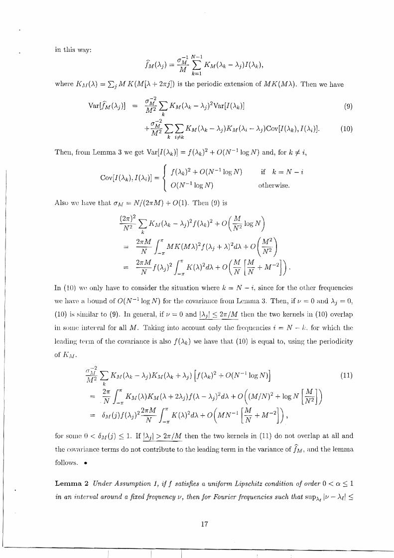
in this way: -1 N-1

~ (JM """" JMP'j) = - L KMP'k - Aj)I(Ak), M k=l

whel'e K!II(A) = ¿j M K(M[A + 27l"j]) is the pel'iodic extension of MK(MA). Then we have

-2

Yal'[fM(Aj)] = ~ ¿ KM(>.'k - Aj)2Yal'[I(Ak)J (9) k

-2

+ i1~ ¿¿KM(Ak - Aj)J(M(Ai - Aj)Cov[I(Ak),I(AdJ· (10) k i#

Then, from Lemma 3 we get Yal'[I(Ak)J = j(Akf + 0(N-1logN) and, fol' k i- i,

j( A )2 + 0(N-1loo' N) if k = N - 'i COV[I(Ak),I(AdJ = k ¡-,

{ 0(N-1logN) otItel'wise.

AIso \Ve llave tllat (JAI = N/(27l"M) + 0(1). Then (9) is

In (10) \V(~ only llave to considel' the situation whel'e k = N - 'i, since fol' the otItel' fl'equencies

\Ve lm\'(~ a l)Qund of O(N-1log N) fol' thc coval'iancc fl'üll1 LClllIlla 3. Then, if l/ = °<1ud Aj = 0,

(10) is similar to (9). In general, if l/ = °and IA.1I :s; 21r/M tIten the two kernels in (10) overlap

in SOllW illtcl'val 1'01' all !vI. Taking into accoullt only tllc 1'rcqucncies i = N - 1,;. 1'01' which thc

Icadill[.!; t('nn 01' the coval'iance is also j(AI.;) we llave that (10) is equal to, using thc pcriodicity

of KM,

-2

~~~ ¿J{AI(Ak -Aj)IC'vI(Ak +Aj) [j(Ak)2 +O(N-1logN)] (11) k

7r = .~ [ 7r K1I1(A)KM(A + 2Aj)j(A - Aj)2dA + O ((M/N)2 + 10gN [~])

O!lI(j)j(Aj)22~M¡:7r K(A)2dA + O(MN- 1 [j~ + M- 2]) ,

fol' SOllW () < OM(j) ::; 1. If IAjl > 27l"/M then the two l,emels in (11) do not overlap at all and

tlle rovmiance terms do not contribute to the leading tenn in the variance 01' lNI, and the Iemma

follows. •

Lemma 2 Under Assumption 1, ij j satisfies a uni.form Lipschitz condition o.f order O< a::; 1

in an 'intcrval around a fixed .frequency IJ, then jor Fourier .frequencies such that sUP>"e Iv - Ael ::;

17

c· 177,-1, {J E {j, k}, for some positive sequence m suclt that l/m + m/N -7 O, uniformly in j and

k, (j,k::/= O),

where dI; p..j) is the discrete Fourier tmnsform of tite series Xl,

N

dx(>..j) = L XtC-iAjt.

t=1

Proof. This lemma is a restatement of, for example, the Lemma in p. 835 of Hannan and

Nieholls (1977), assuming only local eonditions on f. As in thc proof of Lemma 1 wc can fix one

E> O such that, if Iv = [l/-E, l/+E], Aj, Ak E Iu for N big cnough. Defining thc Dirichlet kernel

N iAjcpN(A) = L e ,

j=1

we hav<~ that for j ::/= k, mod (N),

Thcn, ii' j ::/= k, lllod (N),

Now wc dividc thc mnge of intcgration in (12) in thc following intcrvals. First,

I/'.'\~+:~~ IcpN(Aj _ A)cpN(A - AJe) [j (A) - f(Aj )]dAI < , Al !I

using SllPAET" If(A) - f(Aj)1 :s; e 'IA - AjfCl in the intel'val considerecl, and

NexL

\J;:~::~' 'PN(Aj - A)'PN(A - Ak)IJ(A) - f(Aj)]dAI

n:s; e· N- 1 sup ¡cp(A - Adl sup lA - Aj¡a-l :s; c· N I- ,

IA-Ak I:SN-l IA-Ak I:SN-l

sinc<~ the range of integration was of order N- l , Define the set I,/(k,j) as the intcrval 1,/ exeept

the previous two neighbourhoods of radius N-1 around Ak and Aj. Then

r cpN(Aj - A)cpN(A - Ak)[f(A) - f(Aj)]dAIJlv(k,j)

I

:s; e sup lA - Aj¡a-l r IcpN(A - AdldA Iv(k,j) J- 1r

:s; e . NI-a log N,

18

using .e7r I'PN(A)ldA ~ e ·logN. Finally in the complementary set of Iv,

11& 'PN(Aj - A)'PN(A - Ak)[f(A) - f(Aj)]dAI

~ cs~p I'PN(Aj - A)'PN(A - Ak)1 [f(Aj) + .J:¡r f(A)dA] ~ e, v

and the lemma follows in the case j i- k because any of the bounds depends on ] 01' k. If] = k

then we can use the same methods as before together with

to get the desired resulto •

Lemr:na 3 Under Assumption 1, if f satisfies a unifonn. Lipschdz condition of mrier' °< a ~ 1,

in an ú!.tr:'l'val a'f'O'und a .fixed freq'Uency // and if sup'\j,. 1// - A),I ~ c· 'fT/,-1, l' = 1, ... ,q, foro some

pos'Ít'ive sr:quence m such that l/m +m/N -+ 0, then, 'uniformly in jr i- 0, with .11' i- ],.1, T i- T',

(13)

and

E [IT (I(Ajl! ~f(Aj,))] = O(N- n 10gN). (14) 7'=1 j( J,)

Proof. The proof it is immediate in the light of thc Prop().~ition in page 31 of BB and our

Lcnnllct 2, as by the Gaussiallity of X t only cumula11ts of areler two of the discrete Fourier

tra11sfol'll1 of X t bave to be considered. Bere the bouncl in (14) is only O(N- n 10gN) and 110t

tIris bOIl11c1 to tIre power of q as in BB. TIre problem \vith their proof is the fol1owing. At the

bcgill11ill¡.'; of their page 33, for k E 1/2 in their notation, CUlll {([2; (Akl), d,r: (Ak2)} N- 1 = O( 1) at

most, b(~('ctuse we can have Ak1 = Ak2 for aH elements in one of the possible partitions. Then,

the se('oncl bouncl in the third fuH paragraph formula of the same page is only O(1) and tIre first

one is O(N-O: log N)(actually O(N- 1) under their conditions), since we have #//1 ~ 1. •

\V(~ give now sorne lemmas needed for the proof of Proposition 1.

Lemma 4 Under Assumptions 1, if f satisfies a uniform Lipschitz condition of arder O < a ~ 1,

in an interval around a fi:red freq'Ueney //, Iv = [// - E, // + E] for some E> 0, then for frequeneies

1Aj = 2íTj /N, ] i- °sueh that sUP.\j 1// - Aj 1 ~ e· m- , for some positive sequence m sueh that

l/m + '11I/N -+ 0, uniformly in j i- 0,

lim sup I(Aj) ~ 210g N sup f(>") w.p.1. N --+00 .\j .\Elv

19

Proof. We can proceed as in the proof of Theorems 4.5.1 and 5.3.2 of Brillingcr (1975), taking

the mean of X t as zero, since we do not include the zero frcquency. In our case, since X t is a

Gaussiall series and j -=1 O, a11 the cumulants of order bigger than two are zero. From Lemma 2

we can obtain, uniformly in j, for m big enough,

Then, for Aj E Il~ and any e and one E as sma11 as we want, from Gaussianity, as N ---+ 00,

Next,

L Eexp {e IRed,r,(Aj)l} AJElv

< L exp{H22nNf(A,i)(1 +E)/4} AJ Elv

< 2exp {lag N + rP2nN sup f(A)(l + E)/4}. AEI"

Now rlcfüw. for 8 > O

(1,2 = 2n(1 + E)(2 + il)N lag N� sup f(A). AO"

Tlwn

Taking

e= (1, [2nN(1 + E)� sup f(A)] -1 1

AE]"

this is ll'sS 01' equal than

USillg lItis last line and the Borel-Cante11i Lemma, as E and á were arbitrary, we obtain that

1/2

lim supIRedx (Aj)I/[2nNlogNp/2:::; [SUPf(A)] w.p.l. N---+oo Aj� AEI"

A similar result is possible for the imaginary part of dx alld then the lemma fo11ows from

20�

Lemma 5 Under Assumptions 1, 2, 3, 4, for frequencies J..j = 27fj IN such that SUPAj Iv - J..jl :S

e . m -1, for some positive sequence m such that 11m + miN ---+ O, uniformly in j,

Proof. Define the weighted autocovariance spectral estimate corresponding to the continuous

average in 1M, when the mean of Xt is known, (and assumed to be Owithout 10ss of generality) ,

where J(!l!(') = MK(M·) periodically extended and

:Y(k) = N- 1 :L XtXt+k'

l'5: t ,t+k'5:N

This estilllate is unfeasible if the mean of tho series is ull1mown, but we on1y need its definitioll

fol' t1l<~ proofs. Now we have, proceeding as in the proof of Theorem 2.1 of RobillSOll (1991),

(15)

(16)

(17)

Ko\\' (lG) is less 01' equa1 thall (see, Hübillson, 1001, p. 1353),

1'~<~;}(;I) 1111N - ,)1 ~ Op (W'~ I"'(~) Ilrl)

1\' )Op N- 1Mo.l( 1".1 1-0. + N- 1M 2 10g N

(

Op(N1-aJ.¡r + N- 1l\12 10gN) = op(I),

USillg Assumption 4 (o: > i) and the fact that :Y(N - T) is a sum of r terms whose mean exists

and is llniform1y bounded. Next (16) is not bigger than

(2W)-1 %: 1'" (~) 111(r) - EI1(r)]f ~ Op (%: 1'" (~ )IN'f: )

= 01" ( N~ M) = 01"(1),

bccausc Assumptions 2 and 4, and Lemma 7 be10w. Finally (17) is bounded by

(18)SlIP li7r

7r J(M(J..j - w) {E[I(w) - f(w)]} dwl J

(19)+ s~p I/n K(w) {f(J..j - wlM) - f(w)} dwl· J

21

Denote by <I>N Fejér Kernel <I>N(.>-) = (21rN)-11'PN(A)1 2 . Similarly to Lemma 2, we have that in

(18) w lies in the interior of Iv as M -+ 00 due to the compact support of K, and fol' fixed O> O

small enough,

sup IE[I(w)] - f(w)1 < sup I r <I>N(a - w)[f(a) - f(w)]dalwE~ wE~ J- w

< sup 1f'(w)1 r I<I>N(a - w)lla - wlda wElv Jlw-al~o

+ sup r I<PN(a -w)I[f(a) + f(w)]da wElv J1w-al>o

O(N-1logN) + O(N-1)

O(N-1log N),

unifonnly in w E IIJ' so (18) is O(N-1logN), since I IIC'II(cy)ldn~ < oo. Next, as M -+ 00, (19)

is boullded by (denoting by A* a value between Aj and Aj - wjM),

1S~l,P / K(w) [f(Aj - wjM) - f(AJ )] dw:::; sl~P / IK(w) lit (A*)11 e; Idw = O(lvr ),

using tIte Cülllpact SUPPOl't of K amI that of l' is bOllllclcd in IIJ' •

Lemma 6 Under the Ass'll7nptíons of Lernrna 5, un'iforrnly in j,

sup IfjI(Aj) - f(A,j) , = Op (N- 1M 2 + N~ M + N-1log N + M- 1) . Aj f(Aj)

Proof. Thc pl'oof is cxactly the same as that of Lenllll<L 4 of 1313, using now our Lcmma 5. •

Lennna 7 Uude1' Ass'U:rn]Jtíons 1 and 2, 'l/,n'~lo1'Tnly in T, ]J > 1,

!:=1'.)VarfY(T)] = O N l' ,(

wheTC .:y (o,,) ís thc (lúased) estírnate of the lag-T' (wtocovaríance ,(1') when tite e:¡;jlectatíon of X,

'¿s !,;uo/Un.

;Y(1') = ~ ¿ (Xt - E[X1]) (Xt+r - E[X1])·

19,t+r~N

Proof. From c.g. Anclel'son (1971, p. 452), clenoting as before the Fejér kernel by <I> N,

N Val' [;Y(r)] = ¡Ww ¡Ww <I> N(a - w)(l + e-i(a+w)r).f(a)f(w)dadw,

and nO\v tIte result follows applying Holder inequality twice, with I<I>N(W)¡ = O(N) uniformly in

w, 11 + té-i(a+w)r I :::; 2 uniformly in r and f~w fP < 00 by Assumption 2. •

Proof of Proposition 1. From the proof of Theorem 3.1 in BE the pl'oposition will follow,

using thcir definitions, if we show

'i = 1,2

22

First we have, denoting now aj = aj,M, from the last steps in the proofs of BB,

N

E[Td = 2íT 2: Wm()\j - v)a-j 12:'K(MAk)0(N- 1) = 0(1), j=1 k

and, denoting as IMSE~(v,M) the IMSEm calculated from the modified speetral estimate (1),

2 I "'""" 2 2","""',,,"",,' 1E[T¡J = NMISEm + 2íT ¿ Wm(Aj - v) o-j ¿ ¿ K(MAk)K(MAn)O(N- ) j k n

+2íT2: 2:Wm(Aj -V)Wm(Ai -1J)a.¡Iai12:'2:'K(MAdK(MA1/)0(N-2) j Ji-i k n

+2íT 2: Wm(Aj - v)2o-j 22:'2:'K(MAk)2

j k n

= NIMSE~n + O(rn) + O(rn) + O(mNIMSE/II)

= O(rn N IMSEm ),

sinc(, sup,\.I7lIWm(A)1 = O(rn). Then using IMSEm = O(M/N) we can obtain

1/2TI = Op(IM8Em [m/M] ) = op(IMSEm ),

because '11/)111 --t O. Now, in a similar fashion,

N

E[T2] = 2íT 2: Wm(Aj - lJ) aj22:'2:'I((MA¡,,)J((MAn )0(N-1) = 0(1), j=1 k n

aud as 1Jdore

(Not e tb,ll in DB's cxprcssioll they have N- I illstead of N iu tlw corrcspolldcnt formula, altllOugh

in tlH' sfiltemellts in the main part of their papel' they p;iw tho right bounds). Then N-1T2 =

Op(E\ISE", [m/Njl/2) = op(IMSEm ). Next,

E[T:¡] = NIMSEm + 0([N/Mr 1 NIMSEm ) + 0([N/Mr 1) + 0([N/iVIr 1 M)

= NIMSEm + 0([N/Mr1NIMSEm ),

and rcasoning in the same way as before,

Thcn l{-IT3 = IMSEm + Op(IMSEm [m/M]1/2) = IMSEm + op(IMSEm). Tlw proof for tlw

remaillderterminBB.sexpression(3.2)continuesthesamehere.using now our Lemmas 2, 4

and 5 illstead of their referenc:es, since the bound for the third term in the expansion still holds

for t,he modified (local) cross-validation. •

23

,

,

.

References�

[1]� ANDERSON, T.W. (1971) The Statistical Analysis of Time Series. Wiley, New York.

[2]� ANDREWS, D.W.K (1991) Heteroskedasticity and autocorrelation consistent covariance

lllatrix. Econometrica 60, 953-966.

[3]� BELTRAO, KI. and BLOOMFIELD, P. (1987) Determining the bandwidth of a kernel

spectrum estimate. Joumal of Time Series Analysis 8, 21-38.

[4]� BRILLINGER, D.R. (1975) Time Series: Data Analysis and Theory. Holt, Rinehart and

Willston, New York.

[5]� BROCKMANN, M., GASSER, T. and HERRMANN, E. (1993) Locally adaptive bandwidth

choice fOl' kernel regressioll cstimators. Joumal of the A1fI,C'l"ica.n Statistical Association 88,

1302-1309.

[6]� BÜHLMANN, P. (1996) Locally adaptive lag-wilHlow spcctral cstimation. JOll'l"Iwl of Túnc

Sr:/'ics Analysis 17, 247-270.

[7]� D(~ll IIAAN, W.J. and LEVIN, A. (1996) A practitioncrs gllide to robust covariance llla­

trix ('stilllation. Discussion Paper, Departll1cnt 01' ECOllOll1ics, Ullivcrsity of California, San

[8]� HANNAN, E.J. amI NICHOLLS, D.F. (1977) Thc estilllation of the predietioll error vari­

aJl(·('. JO'll'f'TW.l of the AmeTican Stat'istical Assocúttio71 7'2, 8~l4-840.

[9]� HlTTIYICH. C.M. (1985) Data drivcll choice 01' a spcCtl'\llll estimate: cxtcllding thc appli­

<:ilbility of cross-validation lllethods. JouT1wl of the A'l/I,cT"ican Statistical AssoC'Íation 80,

9:n-U...l0.

[10]� HERRMANN, E. (1997) Local bandwidth choice in kernel regression estimation. Joumal of

COllljJlltational and Gmphica.l Statistics 6, 35-54.

[11]� HURVICH, C.M. and BELTRAO, KI. (1994) Automatic semiparametric estimation of the

lllClllory parameter of a long-memory time series. JouTnal of Time Series Analysis 15,

2S:J-:Hl2.

[12]� LEPSKII, O.V. and SPOKOINY, V.G. (1995) Local adaptivity to inhomogeneous smooth­

lWSS.l. Resolution Leve!. Preprint.

24

[13]� NEWEY, W.K. and WEST, K.D. (1994) Automatic lag selection in covariance matrix esti­�

mation Review 01 Economic Studies 61, 631-653.�

[14]� nOBINSON, P.M. (1991) Automatic frequency domain inference on semiparametric and�

nonparametric models. Econometrica 59, 1329-1363.�

[15]� WAHBA, G. (1980) Automatic smoothing of the log periodogram. Journal of the American�

Stati8tical Association 75, 122-132.�

25�

Table 1 M minimizing IM8Em (O, M)

MüDEL 1 MÜDEL 2 MÜDEL 3 MüDEL 4 MÜDEL 5

I\;f*(0): 7.158 7.131 20.340 11.076 11.969

III band M bias M bias M bias M bias M bias

1 129 7.00 -0.16 24.00 16.87 14.50 -5.84 12.00 0.92 12.25 0.28

1.02 125 7.00 -0.16 24.50 17.37 15.50 -4.84 13.00 1.92 12.25 0.28

l.()(j 121 7.00 -0.16 24.50 17.37 15.50 -4.84 13.00 1.92 12.25 0.28

1.09 117 7.00 -0.16 24.50 17.37 15.50 -4.84 13.00 1.92 12.25 0.28

1.13 113 7.00 -0.16 25.00 17.87 15.50 -4.84 13.00 1.92 12.25 0.28

1.17 109 7.00 -0.16 25.00 17.87 15.50 -4.84 13.00 1.92 12.25 0.28

1.21 105 7.00 -0.16 27.50 20.37 15.50 -4.84 13.50 2.42 12.00 0.03

1.26 101 7.00 -0.16 27.50 20.37 15.50 -4.84 13.50 2.42 12.00 0.03

L.B 97 6.50 -0.66 27.50 20.37 15.50 -4.84 13.50 2.42 12.00 0.03

1.:37 93 6.50 -0.66 27.50 20.37 15.50 -4.84 13.50 2.42 12.00 0.03

1.-1:) 89 6.50 -0.66 27.50 20.37 15.50 -'1. 8-1 13.50 2.42 12.00 0.0:3

LíO 85 1.50 -5.G6 28.00 20.87 15.50 -4.84 13.50 2,42 12.00 o.en 1.;)1-) 81 1.50 -5.66 28.00 20.87 lS.S0 -4.84 13.50 2.42 1~.00 0.03

1.(¡G 77 1.50 -S.66 28.00 20.87 15. SO -4.8:1 13.50 2.42 1:2.00 0.03

1. 76 73 4.00 -3.16 28.50 21.37 15.50 -4.8-1 13.50 2.42 12.25 0.28

Loe) 69 4.50 -2.66 28.50 21.37 16.50 -3.84 14.00 2.92 12.25 0.28

1.!), 65 5.00 -2.16 28.50 21.37 16.50 -3.8:1 14.00 2.92 12.25 0.28

2.0D 61 6.00 -1.16 24.00 16.87 17.00 -3.3:1 14.00 2.92 11.25 -0.72

2.2-1 57 6.00 -1.16 24.00 16.87 17.00 -3.34 14.00 2.92 11.25 -0.72

2.11 S3 6.50 -0.66 23.00 15.87 17.00 -3.31 u.no 2.92 11.2S -0.72

2.(jl cID 6.50 -0.66 23.00 lS.87 17.()O -3.3-1 14.00 2.92 11.00 -0.97

2.0-1 45 6.50 -0.66 22.50 15.37 17.00 -3.34 14.00 2.92 9.50 -2.47

:\. l2 41 G.OO -1.16 15.00 7.87 1.50 -18.8-1 12.50 1.42 3.00 -8.97

:3.·1;) 37 6.00 -1.16 13.50 6.37 1.50 -18.84 12.00 0.92 3.00 -8.97

3.87 33 5.50 -1.66 12.00 4.87 1.50 -18.84 11.00 -0.08 :3000 -8.97

4.-11 29 5.00 -2.16 10.00 2.87 1.50 -18.84 11.00 -0.08 2.75 -9.22

5.12 25 4.00 -3.16 9.00 1.87 1.50 -18.84 10.50 -0.58 2.50 -9.22

6.09 21 3.00 -4.16 8.50 1.37 1.50 -18.84 1.50 -9.58 2.50 -9.22

7.52 17 3.00 -4.16 8.00 0.87 1.50 -18.84 1.50 -9.58 2.75 -9.22

9.84 13 2.50 -4.66 7.50 0.37 1.50 -18.84 1.50 -9.58 2.75 -9.22

14.22 9 2.00 -5.16 7.00 -0.13 2.00 -18.34 1.50 -9.58 3.00 -8.97

25.60 5 2.00 -5.16 6.50 -0.63 3.50 -16.84 1.50 -9.58 3.00 -8.97

128.0 1 2.00 -5.16 6.50 -0.63 11.00 -9.34 1.50 -9.58 3.00 -8.97

26

Table JI M minimizing CVLLm(O, M)�

MODEL 1 MODEL 2 MODEL 3 MODEL 4 MODEL 5�

M*(O): 7.158 7.131 20.340 11.076 11.969

m band bias sd mse bias sd mse bias sd mse bias sd lllse bias sd mse

1.11 115 3.42 4.20 29.35 9.54 4.54 111.52 -10.98 4.08 137.08 -0.49 3.72 14.10 -0.13 3.70 13.74

1.17 109 3.47 4.22 29.82 9.76 4.59 116.36 -10.85 4.24 135.62 -0.45 3.68 13.76 -0.04 3.85 14.81

1.24 103 3.49 4.19 29.74 9.96 4.57 120.13 -10.74 4.32 134.08 -0.28 3.88 15.11 -0.01 3.94 15.54

1.32 97 3.52 4.27 30.64 10.11 4.67 124.04 -10.74 4.27 133.53 -0.13 4.00 15.98 0.05 3.85 14.84

1.41 91 3.68 4.38 32.69 10.54 4.85 134.69 -10.55 4.37 130.44 0.03 3.99 15.94 -0.06 3.89 15.15

1.51 85 3.80 4.36 33.48 11.01 5.04 146.66 -10.41 4.46 128.19 0.12 4.11 16.90 -0.30 4.05 16.52

1.62 79 3.83 4.36 33.69 11.55 5.52 163.94 -10.34 4.27 125.14 0.32 4.12 17.11 -0.18 4.15 17.22

1.75 73 3.91 4.45 35.09 11.88 5.56 172.01 -10.22 4.38 123.63 0.47 4.09 16.98 0.00 4.44 19.72

1.91 67 3.92 4.63 36.79 12.33 5.67 184.10 -10.05 4.54 121.58 0.74 4.45 20.39 -0.01 4.55 20.71

2.10 61 3.61 5.05 38.56 12.80 6.12 201.33 -9.90 4.52 118.52 0.95 4.53 21.42 0.02 4.76 22.70

2.33 55 3.08 5.62 41.13 13.08 6.55 213.86 -9.73 4.62 116.11 1.19 4.87 25.15 0.11 5.10 26.06

2.61 49 2.80 6.18 46.00 10.83 5.93 152.52 -9.41 4.94 112.97 1.28 4.89 25.49 0.12 5.37 28.83

2.98 43 2.85 6.13 45.74 9.95 5.31 127.17 -9.17 5.08 109.82 1.52 5.09 28.21 0.42 5.68 32.46

3.46 37 2.98 6.23 47.65 6.26 4.64 60.72 -8.66 5.53 105.52 un 5.87 38.12 0.81 6.18 38.88

4.13 31 2.92 6.27 47.85 4.32 4.48 38.69 -8.58 5.57 104.62 2.12 5.68 36.79 -0.27 6.60 43.68

5.12 25 3.02 6.83 55.78 2.97 5.16 35.43 -7.84 6.10 08.70 1.86 6.20 41.01 -1.45 7.11 52.70

6.74 19 -3.58 3.44 24.66 0.87 4.12 17.70 -8.26 6.05 104.87 -4.50 5.25 47.76 -8.14 2.90 74.61

9.85 13 -2.18 3.82 19.32 -0.14 4.01 16.08 -6.64 7.10 04.61 -2.95 6.04 45.25 -7.54 3.04 66.15

18.29 7 0.38 4.65 21.76 0.06 5.51 30.40 -6.85 8.29 115.77 -1.34 6.21 40.33 -4.58 5.31 49.24

128.0 1 9.13 HU9 191.59 4.00 9.41 104.40 -3.97 0.78 111.51 5.54 10.11 1~¡2.0G 4.24 10.08 110.50

27

T1 I I

Table III ¡;¡, ¡ ~ (O)M

MODEL 1 AR(3) el: - [ O 60 -O 60 030]- , , N = 120 M*(O): 6.1516 f(O): 0.3248 Methoel bias sel Rmse bias sel Rmse (sel) MSE ratio

GLOBAL 0.3584 2.1217 0.1224 -0.0177 0.1263 0.1542 (0.0355) 1.2357 1 0.0356 2.3079 0.1408 -0.0194 0.1228 0.1465 (0.0344) 1.1746 2 -0.2734 2.3369 0.1463 -0.0204 0.1191 0.1385 (0.0335) 1.1100 3 -2.8218 1.8509 0.3009 -0.0334 0.0872 0.0826 (0.0253) 0.6618 4 -2.8278 1.8884 0.3055 -0.0406 0.0930 0.0977 (0.0264) 0.7827 I

5 -2.8209 1.7909 0.2950 -0.0397 0.0907 0.0929 (0.0259) 0.7444 6 -2.8381 1.8012 0.2986 -0.0397 0.0905 0.0926 (0.0258) 0.7424 7 8

-2.8488 -1.2422

1.7770 2.4017

0.2979 0.1932

-0.0398 -0.0183

0.0904 0.1171

0.0926 0.1332

(0.0258) (0.0327)

0.7419 1.0678 I

9 -1.1877 2.4329 0.1937 -0.0184 0.1223 0.1449 (0.0335) 1.1618 ITER.1 -1.8846 2.4752 0.2558 -0.0284 0.1135 0.1297 (0.0302) 1.0689 ITER.2 -1.8603 2.4889 0.2551 -0.0275 0.1134 0.1291 (0.0311) 1.0638

I

ITER.3 -1.0683 2.3353 0.1743 -0.0285 0.1148 0.1326 (0.0312) 1.0927 LOCAL -2.7154 2.1030 0.3117 -0.0472 0.0921 0.1016 (0.0276) 0.8375 N = 256 M*(O): 7.1582 f(O): 0.3248 Method bias sel Rmse bias sel Rmse (sel) MSE ratio

GLOBAL 1.2240 2.3207 0.1343 -0.0156 0.0918 0.0821 (0.0269) 1.2578 1 1.0328 2.5056 0.1433 -0.0154 0.0919 0.0822 (0.0269) 1.2593 2 0.2098 2.5265 0.1254 -0.0165 0.0877 0.0754 (0.0257) 1.1553 3 -3.6296 2.1438 0.3468 -0.0308 0.0586 0.0416 (0.0174) 0.6371

I 4 -4.0582 1.8538 0.3885 -0.0383 0.0596 0.0476 (0.0177) 0.7288

G -3.9735 1.7898 0.3707 -0.0387 0.0598 0.0481 (0.0177) 0.7363 () -3.9495 1.7956 0.3673 -0.0386 0.0599 0.0481 (0.0177) 0.7368 7 -3.9461 1.7606 0.3644 -0.0377 0.0604 0.0481 (0.0179) 0.7373 8 -1.2117 2.7952 0.1811 -0.0135 0.0865 0.0727 (0.0253) 1.1136 9 -1.1019 2.9139 0.1894 -0.0123 0.0872 0.0736 (0.0255) 1.1266

ITER.l -1.9004 3.2307 0.2742 -0.0121 0.0864 0.0722 (0.0253) 1.0665 ITER.2 -1.8546 3.2277 0.2704 -0.0120 0.0867 0.0726 (0.0235) 1.0725 ITEILl -0.4209 2.8948 0.1670 -0.0104 0.0876 0.0738 (0.0245) 1.0902 LOCAL -3.7812 1.9504 0.3533 -0.0327 0.0607 0.0450 (0.0186) 0.6651

N = '±so M*(O): 8.1171 f(O): 0.3248 fvIdhod bias sel Rmse bias sr! Rmse (sel) lVISE ratio

GLOBAL 1.7736 2.5416 0.1458 -0.0111 CL0736 0.0525 (0.0308) 1.3254 1 1.6460 2.5955 0.1434 -0.0107 0.0738 0.0527 (0.0309) 1.3304 :2 0.5319 2.7710 0.1208 -0.0121 0.0699 0.0478 (0.0293) 1.2052 3 -4.2811 2.4304 0.3678 -0.0269 0.0412 0.0230 (0.0174) 0.5795 4 -5.2523 1.6165 0.4584 -0.0354 0.0410 0.0279 (0.0173) 0.7031 5 -5.1230 1.6590 0.4401 -0.0365 0.0409 0.0285 (0.0173) 0.7204 ti -5.0873 1.7477 0.4392 -0.0368 0.0406 0.0285 (0.0171) 0.7188 7 -4.9684 1.7539 0.4213 -0.0362 0.0420 0.0291 (0.0177) 0.7340 8 -1.2159 3.3937 0.1972 -0.0118 0.0683 0.0456 (0.0286) 1.1495 9 -0.8354 3.3192 0.1778 -0.0071 0.0683 0.0446 (0.0285) 1.1266

ITER.1 -1.8274 3.7082 0.2594 -0.0103 0.0681 0.0449 (0.0282) 1.1118 ITER.2 -1.7917 3.7178 0.2585 -0.0101 0.0680 0.0447 (0.0284) 1.1078 ITER,3 -0.0604 3.1202 0.1478 -0.0106 0.0690 0.0462 (0.0292) 1.1449 LOCAL -4.8619 2.1285 0.4275 -0.0289 0.0429 0.0254 (0.0182) 0.6285

28�

Table IV M, fM(o) MODEL 2. AR(2) a = [0.60, -0.90J

N= 120 M*(O): 6.1285 [(O): 0.0942 Method bias sd Rmse bias sd Rmse (sd) MSE ratio

GLOBAL 4.9919 1.3243 0.7102 0.0144 0.0580 0.4027 (0.2042) 1.4147 1 5.0619 1.3069 0.7277 0.0145 0.0583 0.4075 (0.2054) 1.4315 2 5.0557 1.3236 0.7272 0.0146 0.0582 0.4063 (0.2050) 1.4275 3 4.0417 1.7333 0.5149 0.0157 0.0563 0.3858 (0.1986) 1.3555 4 0.8858 2.2370 0.1541 0.0179 0.0517 0.3378 (0.1825) 1.1867 5 0.5057 2.4880 0.1716 0.0148 0.0481 0.2856 (0.1705) 1.0035 6 0.5049 2.5140 0.1751 0.0148 0.0483 0.2878 (0.1712) 1.0111 7 0.4994 2.5041 0.1736 0.0149 0.0483 0.2879 (0.1712) 1.0114 8 0.5482 2.4251 0.1646 0.0153 0.0483 0.2898 (0.1713) 1.0182 0 1.8352 1.9411 0.1900 0.0163 0.0501 0.3123 (0.1774) 1.0971

ITER..l 1.5649 2.4872 0.2299 0.0198 0.0544 0.3779 (0.0369) 1.3026 ITER.. 2 1.5576 2.5005 0.2311 0.0197 0.0543 0.3767 (0.0365) 1.2985 ITER.3 2.3805 2.0955 0.2678 0.0171 0.0541 0.3624 (0.0364) 1.2493 LOCAL 0.1151 2.7552 0.2025 0.0203 0.0532 0.3656 (0.0345) 1.2603 N = 256 M*(O): 7.1313 f(O): 0.0942 Method bias sd Rmse bias sd Rmse (sd) M8E ratio

GLOBAL 8.8523 2.2880 1.6439 0.00G1 0.0395 0.1802 (0.1403) 1. 7627 1 9.0051 2.2794 1.6967 0.0061 0.0397 0.1822 (0.1411) 1. 7823 2 8.8244 2.3557 1.6403 0.0060 0.0397 0.1820 (0.1410) 1. 7795 :3 5.5188 2.4520 0.7171 0.0068 0.0362 0.1529 (0.1285) 1.4949 4 0.3458 2.9035 0.1681 0.0079 0.0311 0.1157 (0.1104) 1.1317

5 0.0524 3.1556 0.1959 0.0080 0.0309 0.1150 (0.1100) 1.1246

ti 0.0325 3.1302 0.1927 0.0079 0.0309 0.1147 (0.1099) 1.1221 7 0.0752 3.1215 0.1917 0.0077 0.0309 0.1145 (0.1099) 1.1193 8 0.2211 2.9473 0.1718 0.0075 0.0305 0.1112 (0.1084) 1.0872 0 2.3715 2.7299 0.2571 0.0086 0.0336 0.1355 (0.1193) 1.3250

ITER,l 1.6299 3.4685 0.2888 0.0110 0.0356 0.1567 (0.0123) 1.3659 1TER.. 2 1.6644 3.4757 0.2920 0.0109 0.0356 0.1564 (0.0122) 1.3631 ITER..:l 2.7699 3.1770 0.3493 0.0004 0.0351 0.1492 (0.0124) 1.3004 ITERA -0.3036 3.2764 0.2129 0.0151 0.0361 0.1731 (0.0128) 1.5090 N = 480 M*(O): 8.0866 1'(0): 0.0942 ~Ictho(l bias sd Rmse bias sd Rmse (sd) MSE ratio

GLOBAL 12.6044 3.6059 2.6283 0.0036 0.0332 0.1259 (0.1668) 2.3140 1 13.0515 3.6773 2.8117 0.0036 0.0337 0.1296 (0.1692) 2.3813 :2 12.3891 3.7140 2.5581 0.0037 0.0334 0.1272 (0.1676) 2.3372 :3 4.9171 2.7340 0.4840 0.0050 0.0269 0.0843 (0.1350) 1.5490 4 -0.1206 3.4026 0.1773 0.0051 0.0230 0.0624 (0.1155) 1.1461 5 -0.3136 3.6181 0.2017 0.0056 0.0240 0.0688 (0.1209) 1.2635 {j -0.3227 3.6333 0.2035 0.0057 0.0239 0.0684 (0.1204) 1.2564 7 -0.3140 3.5994 0.1996 0.0056 0.0238 0.0673 (0.1195) 1.2368 8 0.0550 3.3089 0.1675 0.0051 0.0228 0.0613 (0.1144) 1.1263 0 2.5597 3.1685 0.2537 0.0066 0.0260 0.0808 (0.1304) 1.4847

ITER,l 1.3475 3.6415 0.2306 0.0068 0.0271 0.0882 (0.0973) 1.6580 ITER..:2 1.3336 3.7227 0.2391 0.0067 0.0270 0.0871 (0.0952) 1.6375 ITER3 2.3780 3.3482 0.2579 0.006 0.0273 0.0888 (0.0943) 1.6678 LOCAL -0.9520 3.6426 0.2168 0.0142 0.0295 0.1206 (0.1142) 2.2668

29

I

I

I

,

•

l

!

I

.

Table V M , ¡M ~ (O) MODEL 3 AR(l) o: -- [O 8J

N -120 M*(O): 17.4803 f(O): 3.9789 Methocl bias sel Rmse bias sel Rmse (sel) MSE ratio

GLOBAL -10.6166 2.0697 0.3829 -1.4331 1.4412 0.2609 (0.0121) 0.7774 1 -10.1789 2.1473 0.3542 -1.3518 1.4883 0.2553 (0.0127) 0.7607 2 -10.0005 2.1871 0.3430 -1.3178 1.5076 0.2533 (0.0127) 0.7545 3 -9.5028 2.2363 0.3119 -1.2429 1.5800 0.2553 (0.0141) 0.7605 4 -8.8514 2.2607 0.2731 -1.1201 1.6132 0.2436 (0.0147) 0.7258 5 -9.0624 2.3161 0.2863 -1.1429 1.6180 0.2479 (0.0146) 0.7385 o -9.0649 2.3162 0.2865 -1.1366 1.6227 0.2479 (0.0148) 0.7386 7 -9.0582 2.3015 0.2859 -1.1340 1.6249 0.2480 (0.0148) 0.7389 8 -9.0917 2.3603 0.2887 -1.1326 1.6280 0.2484 (0.0148) 0.7401 9 -8.9180 2.2433 0.2767 -1.1117 1.6222 0.2443 (0.0147) 0.7278

ITER,l -9.0712 2.3821 0.2879 -1.1887 1.5021 0.2318 (0.0093) 0.7759 ITER,2 -9.0783 2.3805 0.2883 -1.1870 1.5020 0.2315 (0.0093) 0.7750 ITER.:) -8.9235 2.3304 0.2784 -1.1897 1.5045 0.2324 (0.0094) 0.7779 LOCAL -9.5462 3.2002 0.3318 -1.2504 1.6060 0.2617 (0.0106) 0.8760 N = 250 M*(O): 20.3404 f(O): 3.9789 Mcthod bias sel Rmse bias sel Rmse (sel) MSE ratio

GLOBAL -11.8184 2.3282 0.3507 -1.1649 1.0979 0.1619 (0.0049) 0.9156 1 -11.3429 2.5014 0.3261 -1.1021 1.1276 0.1570 (0.0053) 0.8883 2 -10.9801 2.6084 0.3078 -1.0553 1.1523 0.1542 (0.0054) 0.8724 3 -10.1367 2.8909 0.2686 -0.9537 1.2287 0.1528 (0.0066) 0.8645 4 -8.9645 3.1418 0.2181 -0.7780 1.3120 0.1470 (0.0071) 0.8313 [) -9.2336 3.1412 0.2299 -0.8224 1.3033 0.1500 (0.0072) 0.8486 (j -9.2166 3.1803 0.2298 -0.8212 1.3075 0.1506 (0.0073) 0.8518 7 -9.1907 3.2153 0.2292 -0.8163 1.3121 0.1508 (0.0073) 0.8532 t\ -9.1855 3.2708 0.2298 -0.8048 1.3216 0.1512 (0.0073) 0.8555 D -8.9485 3.0693 0.2163 -0.7688 1.3221 0.1477 (0.0074) 0.8358

ITER.1 -9.1750 3.2453 0.2289 -0.8151 1.3555 0.1580 (0.0087) 0.8343 ITErt2 -9.1983 3.2183 0.2295 -0.8139 1.3549 0.1578 (0.0086) 0.8330 ITEre) -9.0201 3.2417 0.2221 -0.8117 1.3581 0.1581 (0.0086) 0.8347 LOCAL -10.4480 4.8921 0.3217 -1.0130 1.5554 0.2176 (0.0105) 1.1489

N = 480 M*(O): 23.0653 f(O): 3.9789 Mcthocl bias sel Rmse bias sel Rmse (sel) MSE ratio

GLOBAL -13.1144 2.5589 0.3356 -0.9397 0.8959 0.1065 (0.0036) 0.8692 1 -12.5516 2.7019 0.3098 -0.8849 0.9133 0.1021 (0.0038) 0.8338 2 -12.0365 2.9481 0.2887 -0.8150 0.9778 0.1024 (0.0047) 0.8355 :3 -11.1065 3.3051 0.2524 -0.7279 1.0481 0.1029 (0.0062) 0.8396 4 -9.2345 3.9710 0.1899 -0.5044 1.2252 0.1109 (0.0114) 0.9052 G -9.8104 3.8532 0.2088 -0.5864 1.1678 0.1079 (0.0093) 0.8804 (j -9.8532 3.7994 0.2096 -0.5827 1.1720 0.1082 (0.0094) 0.8833 7 -9.8316 3.7731 0.2084 -0.5808 1.1713 0.1080 (0.0094) 0.8813 8 -9.7846 3.7902 0.2070 -0.5720 1.1654 0.1065 (0.0089) 0.8690

O -9.1792 3.8624 0.1864 -0.5107 1.2173 0.1101 (0.0111) 0.8985

ITER.1 -9.8240 3.7510 0.2079 -0.6154 1.1623 0.1093 (0.0098) 0.8729 ITER.2 -9.8211 3.7482 0.2077 -0.6128 1.1626 0.1091 (0.0098) 0.8716 ITER.3 -9.6628 3.7257 0.2016 -0.6111 1.1682 0.1098 (0.0097) 0.8771

I LOCAL -11.5117 6.4805 0.321)0 -0.9551 1.4600 0.1923 (0.0149) 1.5361

30

--_._-------------------------------------­

Table VI M, fu(O) MODEL 4. AR(2) a = [ 1.37, -0.68]

N = 120 M*(O): 9.5192 f(O): 1.7109 Methoel bias sel Rmse bias sel Rmse (sel) M8E ratio

I GLOBAL -1.5246 2.0629 0.0726 0.3645 0.8710 0.3046 (0.0133) 1.0897 1 -1.1855 2.1272 0.0654 0.3387 0.8846 0.3065 (0.0141) 1.0966 2 -1.0976 2.1279 0.0633 0.3331 0.8842 0.3050 (0.0137) 1.0912 3 -1.0675 2.4082 0.0766 0.3115 0.8654 0.2890 (0.0113) 1.0340 4 -6.3775 1.6813 0.4800 0.8904 0.7394 0.4576 (0.0094) 1.6372

5 -5.8612 2.3158 0.4383 0.8097 0.7409 0.4115 (0.0093) 1.4722 6 -6.0061 2.2031 0.4517 0.8097 0.7378 0.4099 (0.0093) 1.4666 7 -6.0687 2.1439 0.4572 0.8149 0.7373 0.4126 (0.0092) 1.4760

I 8 -6.2126 1.8765 0.4648 0.8163 0.7271 0.4083 (0.0088) 1.4606 9 -1.2837 2.3808 0.0807 0.3197 0.8686 0.2927 (0.0130) 1.0471

ITER.1 -4.0982 3.1207 0.2928 0.5708 0.8716 0.3708 (0.0125) 1.2816 ITER.2 -3.7176 3.2021 0.2657 0.5359 0.8942 0.3713 (0.0131) 1.2831 ITER.3 -1.3912 2.3026 0.0799 0.3027 0.8659 0.2875 (0.0112) 0.9935 LOCAL -6.8745 1.3891 0.5428 0.6488 0.7208 0.3213 (0.0093) 1.1105 N = 256 M*(O): 11.0767 f(O): 1.7109 Methocl bias sel Rmse bias sel Rmse (sel) MSE ratio

GLOBAL -0.7144 2.4977 0.0550 0.1876 0.6060 0.1375 (0.0031) 1.0817 1 -0.2252 2.6355 0.0570 0.1758 0.6132 0.1390 (0.0029) 1.0939 2 0.0038 2.7185 0.0602 0.1653 0.6149 0.1385 (0.0027) 1.0897 :3 0.0732 3.0833 0.0775 0.1629 0.6193 0.1401 (0.0025) 1.1023 4 -8.5512 1.0325 0.6047 0.7154 0.4864 0.2557 (0.0029) 2.0115

5 -8.1785 1.8234 0.5723 0.7207 0.4880 0.2588 (0.0028) 2.0362 6 -8.2247 1.7684 0.5768 0.7123 0.4908 0.2556 (0.0026) 2.0111 7 -8.2768 1.6320 0.5800 0.7096 0.4874 0.2531 (0.0027) 1.9918 1) -8.2397 1.6825 0.5764 0.7049 0.4914 0.2522 (0.0027) 1.9846 9 -0.2085 2.9149 0.0696 0.1636 0.6025 0.1332 (0.0015) 1.0477

ITER1 -2.2004 4.3069 0.1906 0.2736 0.6748 0.1812 (0.0034) 1.3529 ITER2 -1.8605 4.1901 0.1713 0.2501 0.6725 0.1759 (0.0034) 1.3133 ITER3 -0.3725 2.9226 0.0707 0.1635 0.6198 0.1404 (0.0021) 1.0484 LOCAL -8.5494 1.3252 0.6100 0.5649 0.4803 0.1878 (0.0041) 1.4027 N = 480 M*(O): 12.5607 f(O): 1.7109 J\Iethod bias sel Rmse bias sel Rmse (sel) MSE ratio

GLOBAL -0.1311 2.6874 0.0459 0.1391 0.4795 0.0852 (0.0034) 1.1124 1 0.3434 2.8332 0.0516 0.1358 0.4871 0.0874 (0.0033) 1.1412 2 0.6247 2.9002 0.0558 0.1269 0.4887 0.0871 (0.0030) 1.1379 3 0.5923 3.2458 0.0690 0.1324 0.4918 0.0886 (0.0029) 1.1574 4 -10.2465 0.7777 0.6693 0.6485 0.3618 0.1884 (0.0043) 2.4608

5 -10.0893 1.1308 0.6533 0.6884 0.3637 0.2071 (0.0043) 2.7052 (j -10.1220 0.9528 0.6551 0.6825 0.3633 0.2042 (0.0044) 2.6678 7 -10.1524 0.8978 0.6584 0.6781 0.3624 0.2020 (0.0044) 2.6380 8 -10.0866 1.0434 0.6518 0.6816 0.3671 0.2048 (0.0044) 2.6747 9 0.4940 2.9411 0.0564 0.1251 0.4836 0.0852 (0.0033) 1.1134

ITER.1 -0.5072 4.3563 0.1219 0.1627 0.5008 0.0947 (0.0056) 1.3540 ITER.2 -0.4021 4.2216 0.1140 0.1464 0.4918 0.0899 (0.0051) 1.2853 ITER.3 0.4426 3.1473 0.0640 0.1255 0.4711 0.081 (0.0048) 1.1605 LOCAL -9.9984 1.268 0.6438 0.5786 0.4020 0.1696 (0.0045) 2.4236

31

,-----~__¡_¡____¡-~_;___r---------_,__---I

,

i

, ,

I

Table VII M , ¡ ~ (O) MODEL 5 AR(5) a -- [O 90, -O 40, O30, -O 50, 030]M'

N = 120 M*(O): 10.2862 f(O): 0.9947 Method bias sd Rmse bias sd Rmse (sd) MSE ratio

GLOBAL -3.1082 2.4496 0.1480 -0.1328 0.3708 0.1568 (0.0059) 0.7418� 1 -3.3923 2.4079 0.1636 -0.1364 0.3588 0.1489 (0.0037) 0.7045� 2 -3.5374 2.3912 0.1723 -0.1463 0.3372 0.1366 (0.0018) 0.6462� 3 -4.3022 2.2374 0.2222 -0.1631 0.3219 0.1316 (0.0017) 0.6228� 4 -6.5136 1.9262 0.4361 -0.0979 0.3082 0.1057 (0.0017) 0.5001� 5 -6.3467 2.0432 0.4202 -0.1044 0.3106 0.1085 (0.0059) 0.5135� 6 -6.4044 1.9119 0.4222 -0.1079 0.3096 0.1086 (0.0061) 0.5141� 7 -6.4625 1.8452 0.4269 -0.1108 0.3017 0.1044 (0.0054) 0.4940� 8 -6.4481 1.7389 0.4215 -0.1136 0.2956 0.1014 (0.0056) 0.4797� 0 -4.2181 2.2987 0.2181 -0.1474 0.3456 0.1427 (0.0049) 0.6751�

ITER.1 -5.6377 2.3226 0.3514 -0.1243 0.3065 0.1106 (0.0028) 0.5476 ITER.2 -5.6777 2.2877 0.3541 -0.1262 0.3062 0.1108 (0.0029) 0.5490 ITER.3 -4.1307 2.3309 0.2126 -0.1602 0.3331 0.1380 (0.0019) 0.6838 LOCAL -6.7268 2.1374 0.4709 -0.1482 0.3112 0.1200 (0.0053) 0.5947 N = 256 M*(O): 11.9693 f(O): 0.9947 Methocl bias sd Rmse bias sd Rmse (sd) MSE ratio

GLOBAL -1.8053 2.6174 0.0706 -0.0874 0.2074 0.0971 (0.0073) 0.9079� J -2.3472 2.8392 0.0947 -0.0953 0.2871 0.0925 (0.0071) 0.8646� 2 -2.8374 3.0196 0.1198 -0.1056 0.2714 0.0857 (0.0072) 0.8015� :J -4.9642 2.8509 0.2287 -0.1437 0.2331 0.0758 (0.0055) 0.7087� Ll -7.9976 2.0997 0.4772 -0.1103 0.2311 0.0663 (0.0042) 0.6196� G -7.8982 2.0823 0.4657 -0.1119 0.2269 0.0647 (0.0047) 0.6050� 6 -7.9106 2.0095 0.4650 -0.1151 0.2188 0.0618 (0.0046) 0.5777� 7 -7.9219 1.9699 0.4651 -0.1161 0.2187 0.0619 (0.0046) 0.5793� 8 -7.9024 1.8739 0.4604 -0.1193 0.2098 0.0589 (0.0045) 0.5505� !) -4.8077 3.1417 0.2302 -0.1319 0.2579 0.0848 (0.0053) 0.7929�

ITEftl -6.2025 3.2035 0.3402 -0.1221 0.2450 0.0757 (0.0046) 0.7080 ITER.2 -6.1708 3.2312 0.3387 -0.1269 0.2408 0.0749 (0.0046) 0.7001 ITER.:J -4.5963 3.1678 0.2175 -0.1328 0.2584 0.0853 (0.0048) 0.7979 LOCAL -8.3630 2.4637 0.5306 -0.1619 0.2388 0.0841 (0.0057) 0.7865 N = L1I)0 M*(O): 13.5727 f(O): 0.9947 l'vlcthod bias sd Rmse bias sd Rmse (sd) MSE ratio

GLOBAL -1.3650 2.6292 0.0476 -0.0555 0.2484 0.0655 (0.0098) 0.9414� 1 -1.6950 3.0532 0.0662 -0.0563 0.2460 0.0644 (0.0098) 0.9260� 2 -2.2844 3.3601 0.0896 -0.0651 0.2389 0.0620 (0.0094) 0.8917� ~¡ -6.2928 3.2159 0.2711 -0.1293 0.1736 0.0474 (0.0070) 0.6815� 4 -9.4970 2.1434 0.5145 -0.1158 0.1638 0.0407 (0.0064) 0.5849� G -9.4377 2.1885 0.5095 -0.1131 0.1649 0.0404 (0.0064) 0.5811� G -9.3505 2.1854 0.5005 -0.1131 0.1619 0.0394 (0.0065) 0.5670� 7 -9.3790 2.0884 0.5012 -0.1148 0.1570 0.0382 (0.0064) 0.5499� 8 -8.8408 2.6853 0.4634 -0.1119 0.1502 0.0354 (0.0061) 0.5099� 0 -4.7637 3.9881 0.2095 -0.1081 0.2097 0.0563 (0.0078) 0.8094�

ITER.1 -6.0425 4.3909 0.3029 -0.1176 0.2023 0.0553 (0.0043) 0.7600 ITER.2 -6.0598 4.2327 0.2966 -0.1170 0.2027 0.0554 (0.0084) 0.7606 ITER.3 -4.4998 3.7678 0.1870 -0.1189 0.2087 0.0583 (0.0085) 0.8010 LOCAL -10.0589 2.4984 0.5831 -0.1767 0.1718 0.0614 (0.0071) 0.8430

32

Table VIII 1(>-), >- E [-11",11"J� Sample size: N = 120 N = 256 N = 480�

Model m IMSE sd IMSE sd IMSE sd�

2� 1 0.13646 (0.09833) 0.06545 (0.03223) 0.03805 (0.01531)

2 0.15758 (0.11871) 0.07140 (0.04125) 0.03659 (0.01570)

3 0.13433 (0.09717) 0.06390 (0.03241) 0.03528 (0.01478)

4 0.13528 (0.09387) 0.06436 (0.03126) 0.03503 (0.01540)

3� 1 0.74030 (0.73461) 0.25241 (0.17345) 0.11225 (0.04458)

2 0.60013 (0.58166) 0.23447 (0.14721) 0.11188 (0.04153)

3 0.66356 (0.61461) 0.23208 (0.15650) 0.09898 (0.03938)

4 0.66240 (0.61012) 0.22940 (0.15911) 0.09612 (0.03824)

5� 1 0.20289 (0.16848) 0.09384 (0.08463) 0.04196 (0.02241)

2 0.14133 (0.09355) 0.05981 (0.03302) 0.03116 (0.01396)

3 0.12857 (0.08317) 0.05855 (0.03205) 0.03082 (0.01405)

4 0.13006 (0.08407) 0.06068 (0.03518) 0.03085 (0.01412) 1----- ­

6� 1 0.47824 (0.74073) 0.14747 (0.21982) 0.06533 (0.05338)

2 0.31678 (0.38975) 0.13110 (0.09898) 0.06334 (0.04976)

3 0.29050 (0.39069) 0.12113 (0.09192) 0.05858 (0.04625)

4 0.28964 (0.39775) 0.14747 (0.21982) 0.05835 (0.04717)

7� 1 0.13666 (0.09507) 0.09814 (0.08571) 0.04842 (0.01873)

2 0.15576 (0.11148) 0.10457 (0.05167) 0.05267 (0.02194)

3 0.13401 (0.09333) 0.09938 (0.04939) 0.05180 (0.01943)

4 0.13444 (0.09171) 0.09809 (0.04800) 0.04991 (0.01980)

33

Modcl 1. AR(3) .(j. - .0, ." Muu~1 2. AR(2) .t;. -.1 Model 3. AR( 1) .ft

~:¡ f\ I '"

"Tj :: aq"

>:::., ci

I \ I ~

(1)

...... 00

~

CJ)

"O:/f / \ 1 ­

(1) ci�

"..,.�.,n

e:. ~I \ I I I \ I

o.. ci " (1)

~ i=l

i ci

H::> i:!!o "..,.

roO ci CIl \

o .,O' :1 ~I :1 ~ ~

0 0 .0 D.' 0.8 '.2 1.6 2.0 2.4 2.8 '.2 O D O.' 0.8 '.2 1.6 2D 2.' 2.8 '.2 1:> U.O 0.8 L2 1.6 2.0 2.' 2.8 '.2

~

O Model 4. AR(2) 1..-"72. -.t;77 Muu~1 5. AR(5) .n. _.04 •. J. _.~..J

o.. o .;~

CIl

...... .. "..,.

O o

J..

) \ I ~

ci

--;;-~

~o

~~

..;

ci ~

, ci

~

ci

o�

o o.u O., Ll6 L2 , ti 20 2.' 28 , 2 u O.') u., O." 1.2 1.6 2 O 2.4- 2.8 '.2� o

1

r-------r--.........--...,-----.---r---..---"""'T""--.........-.......,,,�

\ N

\ <O

I \

\

\ E \ w VJ ¿

D Q)

o E Vl W

Q)

D o ¿

L....- -'--_----""__---'-_--'__-'-__~_----'- -'N

t¿'O ¿I'O WO tO'O

;5

~

LO

LO

'""., ~

C/

;¡

E w Vl ¿

1) Q)

o E

"'Uí w

~

Oí 1) o ¿

\.D

""

Figure 2: IMSEm(M,O) fol' Model 1.

35

11

1)

1:

1:

1 1

11

11

1

1

I I

I I I I

N

'"

~

(» ,11

OC> N

<Ó <1" N

~

N '-' OC <l:

E W (f)

~

o N

2

TI

2 CJ

.~ U1

W

N

c:; TI CJ 2

_ ---= ;e...c­ -'­

'" -

N ~

ro

t

(Vl)W:JSVlI

.,. O

c~

¿

'"'-' <i: E ~

(f)

~ o (IJ

CJ

E ~

U1 w

N Qj TI o 2

el "'l

Figure 3: IMSEm(M,O) for Model 2.

36

N t'l

\ \ ·.. 1. <Xl

'.1 N

\ \1 '1·

~

ro \ \ I " IN

\\ \ '-' \a::

O< \ :\ N

E l· w I IIf)

~ I

u I :J ::;~ ~ . :1� o

.J'E I I

lfl ~ w / I/ n

/ 1/Qj u ./ o / /;.­:> ./

0'[ 0'<: 0'1

E

u Q) ~

o E

Q)

u o :2

Figure 4: IMSEm(M,O) for Model 3.

37

.......-...,....-.....,...---.--.,.....-.......----,---r----r--....,...-......,.--_-....,...-.....,.--,~

r-­

~

".

'"r-­

Ñ r-­r')

o ~

~ '" f')""~

Ir <i

E w "' ::2-(f)

~ 1J (lJ

o E ;" tí w

.; Oj D o ::2

.,. g'O L'O 9'0 ,'O \'0 ¡"O l'O l'O

(V'I)w3SI"<I

E LJ (f)

:"

(lJ

1J o ::2

Figure 5: IMSEm(M,O) [al' Model 4.

38

r-_...,.._--,__........_--.-__,....._...,.._........__.,......._......_--,r--_...,..._--r__.,...._....,~

o N

~_.

v'l O'l

r')

ú1

r: v

m

ú1 ~

er: <t

E w V1

~ 1)

" ~

o E -¡¡; w

úl I"l O; C'\ 1)

o ¿

8'(;

Figure 6: IMSEm(M,O) for Model 5.

39

N

'" ~

n "­\ \ ro <O N

I \ \

"­<O

"" \

.,. "" N

~ "­n './

eL \ « "­"­O O

O \ N\ O

\ ::i "­I

w ~ \ " ::;:~ :J \ "­O \w f- \ \« O \ ::i \ \

-N

«

\> \ I/l \ \Vl O ro\Q::

u \ \

I \

\ .,.O!

¿ \ TIO

.---/

/

\ ~ O

0009 0001' OOOZ O OOOZ- 0001'- 0009­

wllfl:)

n

<:i I

L)

~

'l

"4' ::::

~

n

'­-« O ::i « > I/l� Vl� O

u

Qj TI o

::;:

O'l

Figure 7: CVLLm(M,O) for Modell.

40

I

N n

~

Ol ',\ \\

\ ro

\ \\

\ N

<O

\ \ \

\ N

~ ... N '-" cr: « \ \

\ \

O \O , \ \ O

NO \

-.J \ \

w \ \

~

:::i \ I \ '3. ¿ \

w If- I \ O

« IO

~ I I \ ~ > J

(f) f \(f)

O/

I cr:

/ /

/ Iu

N/ I /

U; /'

'O ./ /' ./O ./ ¿ ,--'

--' -/c.:.­

O

0'9 S'S O'S S', o', s'r o'r S'l O'l S'I O'l

,O l x (~)wllit)

~

G1

<O

'-" " cr: « o O�

º­u ~

:::i O� L..J� f­« O -.J « > (f)� (f)'�

O cr: U

N

U;� 'O� O� ¿�

9

Figure 8: CVLLm(M,O) for Model 2.

41

-------------

I

,

'J [( <!

o o o

...J W ~

:::J

o W f­<! o ...J <! > V> V> o r:: u

" D o ::;;

ro

" « G o o

'é ...J

o CJ f­<! C;

...J <! > V> \f)

o [(

u

".,

Qj D o ::;;

\ \ \

I \I \ I \\'\ I I

\ \ \\

\ \\ \"\ \ \ \ . \ \

.. \ \ \ \ I\

., \ I \\ I\\ \

,\ I \\ \ IVI I \\ \\\ \ I \

I I I\

l\

I I I I ,,1

I I I I

\

I I

I 1I I I

,/ II

/ ........ /

// / / /�

~ .;::-:-- ..-- //'

:..--- -- .-/ / /

\'\ O'l 6'0 g'O ro 9'0 s'o t'O n ,0 \ x (V-<)WllI\J

s'O \1'0 \:,0

6'0 'tro CO 9'0 O'l ~ \1°\ xl'l ~ \10 \sO l

Figure 9: CVLLm(M,O) fol' Model 3.

42

<Xl

'"

..� '"

o '"

o l'O

.---........,._....,..._....-----,-.....,...-..,....--...---.--....,....-.,....-........,.--.--...,..--r--.....,...--r--..-------.~

<O N

... N

o N

N

...

Figure 10: CVLLm(M,O) for Mode14.

43

r--.....----,---.---..,.----,------;--..---...,-----.,.--,....--.....----,---.-----,~ '")

Lf)

I \ \ '") \ \

\ \

'<t \ \ I \ \\ \e:

I \\ I ~ \ \

oo:: N <: \ \ o o \ \ o \ \� I� ::J I \� w \ \ ~

o..J

\ 1 \

NI

f- 1 \

W

<: \ I

..J Iº<: I\ I> (f) I

II(f)

o CL u I /

I / tri I /�Qi / /� u ­o :2

1­

,01 x (Vi)wll!\J

'")

ln ~, I

"l

.;

ey,

ú) ~

r~

~ ~

O

u ~

..J

O l..:..J� f­<:

..J º<:, > (f) (f)

O e.­U�

tri� Qi� TI o :2

Figure 11: CVLLm(M,O) for Model 5.

44