Learning about compliance under asymmetric information

Carmen Arguedas* and Sandra Rousseau**

* Universidad Autonoma de Madrid

** CEDON – KU Leuven

CITE AS: Arguedas, C. and S. Rousseau (2012). Learning about compliance under asymmetric information. Resource and Energy Economics, vol.34(1), p.55-73.

(Doi: 10.1016/j.reseneeco.2011.09.001)

Abstract

Over time, inspection agencies gather information about firms’ pollution levels and this information may allow agencies to differentiate their monitoring strategies in the future. If a firm is less successful than its peers in reducing emissions, it faces the risk of being targeted for increased inspections in the next period. This risk of stricter monitoring might induce high-abatement cost firms to mimic low-abatement cost firms by choosing lower emission levels, while the latter might try to avoid being mimicked. We explain firms’ compliance decisions and the inspection agency’s monitoring strategy by means of a signaling game which incorporates dynamic enforcement and learning. Interestingly, we show that the ongoing signaling game between firm types might lead to firms over-complying with the emission standard.

Keywords: Monitoring and enforcement; pollution; learning; signaling.

JEL codes: D82, H83, K42.

2

I. INTRODUCTION

Firms’ compliance status with environmental rules is sometimes affected by that of other firms. For example, in the US pulp and paper, chemical or petroleum industries, there exists empirical evidence that the compliance status of one firm positively depends on the compliance record by rival firms located in the same state, see Decker and Pope (2005). This suggests that pollution reductions by one firm influence further pollution reductions by other firms, so that compliance decisions might be seen as strategic complements. Decker and Pope (2005)’s explanation for this phenomenon relies on the fact that increased compliance by one firm reduces enforcement resources allocated to that firm and increases resources allocated to its rivals, thus increasing rivals’ compliance rates.

The purpose of this paper is to provide an alternative explanation for this empirical observation. Decker and Pope (2005) consider a static setting and explicitly model the enforcement part of the regulation. We instead concentrate on the dynamic influence of firms’ past compliance status on future regulations. The reason is that a lot of empirical evidence exists to support the fact that inspection agencies impose more stringent enforcement policies on those firms polluting more. For example, Nadeau (1997) finds for the US pulp and paper industry that both the probability of inspection and the probability of enforcement actions depend positively on the potential amount of emissions; for the US chemical and pulp and paper industries Decker (2005) shows that plants which produce less TRI chemical releases per unit production are less likely to be inspected than plants which produce large TRI chemical releases; Gray and Deily (1996) find for the US steel industry that regulatory actions depend on tons of emissions produced; Eckert (2004) shows for petroleum storage sites in Canada that inspections depend on the number of tanks at an installation; Rousseau (2007) shows for the Belgian textile industry that inspections depend on the potential amount of emissions, proxied by the firm’s capacity; Stafford (2002) finds for the US hazardous waste regulations that inspections depend on the (log of) tons of waste generated; among others.

Since inspection agencies and polluting firms interact overtime, the former collect information on firms’ types by performing audits and measuring emission levels. Since enforcement resources are scarce, the monitoring strategy in subsequent periods is then determined not only by the firms’ past compliance status, but also by their performance relative to the other firms. This acts as a signal of the firms’ types, since a firm that is less successful in reducing pollution faces the risk of being targeted for increased inspections in the next period.

The interaction between firms’ relative emission levels and future inspections implies an interesting signaling game. Forward looking firms with higher abatement costs might be tempted to choose sufficiently low levels of emissions (i.e., mimic low-cost firms) in order to face laxer enforcement in the next period. But, at the same time, low-cost firms might try to prevent being mimicked by high-cost firms in order to be treated as a group with enforcement privileges. As a result, actual emissions might be considerably lower than those expected in a static (or one-period) regulatory process. In fact, this process may even lead firms to do better than legally required, i.e. they might over-comply with the regulation in place.1

1 Among others, Arora and Gangopadhyay (1995), Maxwell et al. (2000), Bagnoli and Watts (2003), Lyon and Maxwell (2003, 2004), Shimshack and Ward (2008) and Wu and Wirkkala (2009) have provided alternative reasons of over-compliance with existing regulations.

3

Our signaling game results in three possible equilibrium outcomes: (i) a separating equilibrium where the threat of mimicking is absent; (ii) a separating equilibrium where low-cost firms actively prevent being mimicked by high-cost firms; and (iii) a pooling equilibrium where all firms choose the lowest possible emission level, in the spirit of Kreps and Sobel (1994). A separating equilibrium (in either case (i) or (ii)) allows the inspection agency to learn the type of additional firms and use the acquired information in the following regulatory period.

Interestingly, we show that the agency is able to induce each specific type of equilibrium by adapting its inspection strategy. The agency trades off two counteracting effects. Firstly, it can use the information previously obtained and focus on firms it knows will generate high returns in the current period. Or secondly, it can try to gather information on unknown firms and thus increase future payoffs. A separating equilibrium is shown to be more likely under a low inspection probability. After all, the smaller the inspection probability, the smaller the expected gain a high-cost firm can get from pretending to be of the low-cost type. Similarly, increasing the inspection probability ultimately makes the incentive of the high-cost firms to imitate the low-cost type so strong that low-cost firms cannot do anything to avoid it and a pooling equilibrium ensues.

We assume that agency’s decisions are based on concerns with regulatory compliance as well as (to various extents) on the level of the associated firms’ abatement costs (see also Harford and Harrington (1991) or Keeler (1995)). A nice implication of our study is that governments can use monitoring budgets to correct agencies’ strategies when agencies’ objectives depart from the strict social cost viewpoint. For example, it is possible to move a strictly enforcing agency (that is, one only concerned with firms’ compliance, but not at all with firms’ abatement costs) from inducing the pooling outcome to a separating outcome by sufficiently restricting the agency’s budget.

Clearly, firms’ heterogeneity with respect to their compliance costs is a key assumption in our context. Although this assumption is known to be important, it has also been generally neglected in the literature (for a notable exception see Raymond (1999)).2

Surprisingly, the explained signaling game through which the agency can learn the type of additional firms and use the acquired information in future regulatory periods has not been explored in the literature on monitoring and enforcement as of yet. Generally, the existing literature does not address the possibility that firms’ compliance decisions might be strategic and, therefore, our proposed signaling game is new in this context.

The signaling model we propose is necessary because we want to stress the combination of (i) over-compliance, (ii) mimicking and/or mimicking prevention, and (iii) targeting of “discovered” big polluters, and existing models are not able to capture these three characteristics together. On the one hand, there exist previous models in the literature (such as Harrington (1988), Raymond (1999), Harford and Harrington (1991), Friesen (2003), or others) showing that budget constrained regulators distribute inspections in response to compliance information thus prompting increased compliance. However, in all these studies firms are assumed to undertake a discrete decision whether to comply or to violate the regulation, and then be moved to the “bad” group in case of non-compliance. The issue of

2 However, learning can be possible even in a context of a single regulated firm. For example, Costello and Karp (2004) show the way regulators can learn firms’ abatement costs through the use of dynamic taxes and quotas, although the signaling issue is absent there as well.

4

mimicking or mimicking prevention (and, thus, the issue of over-compliance) cannot be explained in that context: if, for example, the dirty firm decides to comply, the clean firm cannot distinguish itself from the dirty one since over-compliance is not a possibility in that context. In the present paper, however, the firm pollution decision is a continuous variable and, thus, there is room for mimicking/ mimicking prevention. The inspection agency penalizes non-compliance (it charges fines), but monitoring in the following period is directed mostly to those violating more (i.e., those polluting more).

On the other hand, Denicolò (2008) presents a signaling model to explain over-compliance with a different purpose that ours. Denicolò (2008) considers a two period model of an asymmetric duopoly, where the more efficient firm may voluntarily over-comply before a stricter regulation is enacted in order to signal that compliance is not too costly. If the government reacts by adopting a stricter regulation, the more efficient firm gains by raising its rival’s costs. Therefore, Denicolò (2008) is not concerned about targeting enforcement and the issue of mimicking cannot be explained in that context either. In that paper, the regulatory policy is uniform for all firms and discrete: the regulator can either force all firms to adopt a good technology (in which case firms must comply) or let firms freely choose which technology to use. A low-cost firm might decide to over-comply (i.e., adopt the good technology when it is not forced to do so) to signal that compliance costs are low thus inducing the regulator to tighten the regulation in the next period (and therefore increasing rivals’ compliance costs). However, a high-cost firm would never like to imitate a low-cost firm decision, since this would only cause larger compliance costs and a tightening of the regulation in the following period.

The main difference of our model versus the traditional models on signaling, such as Spence (1973), Rothschild and Stiglitz (1976) and Grossman (1981), is that in ours several firms emit simultaneous signals that can be used by the regulator to update its information about the firms and set the regulatory strategy in the subsequent period, as opposed to the case of a single firm emitting a single signal.3 In our model, the combination of multiple signals allows the regulator to revise its information about the regulated firms. Obviously, if all audited firms send the same signal, the regulatory agency gets no useful information out of its inspection activities.

The remainder of the paper is organized as follows. In section 2, we present the model. In sections 3 and 4, we respectively derive the results of the second and first regulatory periods. In section 5, we discuss on the implications of our model. We conclude in section 6. All the proofs are in the Appendix.

II. THE MODEL

We consider an industry composed of N firms that emit pollution. The emission level of firm i in period t is denoted as 0,ti ie e e⎡ ⎤∈ ⎣ ⎦ , where 0e ≥ is the lowest possible emission level associated with implementing the best available technology (or the absolute minimal level required for the firms to continue to do business) and o

ie is the emission level without

3 Signaling games have been previously used in a monitoring and enforcement setting by Reinganum and Wilde (1986) and Sobel (1989). These studies model settlement and prosecution decisions and show that plaintiffs with a strong case demand relatively higher payments in order to settle out of court.

5

regulation in place with o oL He e≤ . The aggregate emission level in the industry in period t is

denoted as t tii N

E e∈

=∑ and causes per period environmental damages represented by the

function ( )tD E , with the usual assumptions ( )' 0tD E > and ( )'' 0.tD E ≥

In each period, each firm in the industry can reduce its emissions at a cost, which depends on the emission level, and also on a parameter iθ , which defines the firms’ type. We assume that the abatement cost function of firm i is ( ),i tic eθ , and that it has the usual specification:

( ), 0e i tic eθ < for all 0ti ie e< , ( ), 0ee i tic eθ > for all 0

ti ie e≤ , and negligible third derivatives. For

simplicity, we consider two types of firms: high-cost firms ( )Hθ and low-cost firms ( )Lθ ,

such that H Lθ θ> . The number of high-cost (low-cost) firms is represented by HN ( )LN ,

such that H LN N N+ = . Also, ( ) ( ), ,L tL H tHc e c eθ θ< , ( ) ( ), ,e L tL e H tHc e c eθ θ> and

( ) ( ), ,ee L tL ee H tHc e c eθ θ≥ .4

We assume that there is a regulation in place, which imposes a uniform emission limit or a standard ( )e e> on the firms.5 The stringency of the standard and the associated fine, in case a firm is discovered exceeding the standard, are determined by law. For simplicity, the fine is assumed to be linear:6

{ }max 0; , 0.tiF f e e f= − >

Further, there exists an environmental enforcement agency whose job is to maximize compliance (or minimize environmental damages) balanced by concerns about firms’ abatement costs.7 This agency has a budget 0tB > per period (say, per year) to spend on

4 Among other specifications, a quadratic abatement cost function satisfies these properties. Moreover, our assumptions ensure that the single-crossing property holds. This implies that high-cost firms find reducing emissions more costly than low-cost firms. 5 Uniform emission standards are commonly used in practise. For example, the US Clean Water Act establishes uniform water pollution discharge limits independent on firms’ location. Noise regulations are often designed as uniform standards, such as the Belgian noise regulation for music in public and private institutions and companies. The national ambient air quality standards included in the US Clean Air Act are largely identical for the whole country. Bans on certain substances, such as CFCs or the use of oil-based paints in urban areas in the US, are by definition uniform standards. Etc. 6 In practice, a linear specification of fines is often encountered for civil fines, since this structure is easy to understand by firms, citizens and administrations. Also, we implicitly assume that the level of the fine is limited. The use of limited fines has been explored by several authors and several possible motivations have been developed, such as the presence of risk aversion (Polinsky and Shavell, 1979), when firms have limited wealth (Cohen, 1987; Polinsky and Shavell, 1991), when there are administrative costs associated with sanctioning (Shavell,1987 and Polinsky and Shavell, 1992), or in the presence of regulatory errors (Nyborg and Telle, 2004; Rousseau 2009), among others Also, in order to preserve marginal deterrence, Shavell (1992) and Mookherjee and Png (1994) argue that fines should be an increasing function of the severity of the violation(s), and thus maximal fines are not optimal. 7 Deterrence can simply mean inducing firms to comply with statutes, which might not necessarily be linked to minimizing damages. For example, regulators may simply want to increase compliance to demonstrate to the public that they are doing their enforcement job. However, in our context, maximizing deterrence and minimizing damages are equivalent objectives. This is so because the compliance/non-compliance decision is a continuous variable, compliance can be defined as the sum of all firms’ violation sizes (i.e., firms’ emission levels minus the emission limit, which is exogenous) and environmental damages are increasing in emissions.

6

monitoring. We assume that the cost per inspection is 0m > and that monitoring is perfectly accurate.8

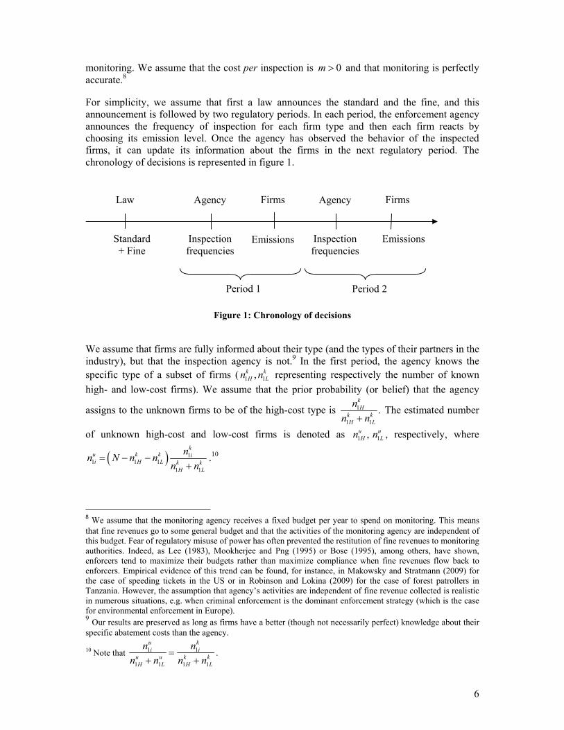
For simplicity, we assume that first a law announces the standard and the fine, and this announcement is followed by two regulatory periods. In each period, the enforcement agency announces the frequency of inspection for each firm type and then each firm reacts by choosing its emission level. Once the agency has observed the behavior of the inspected firms, it can update its information about the firms in the next regulatory period. The chronology of decisions is represented in figure 1.

Figure 1: Chronology of decisions

We assume that firms are fully informed about their type (and the types of their partners in the industry), but that the inspection agency is not.9 In the first period, the agency knows the specific type of a subset of firms ( 1 1,k k

H Ln n representing respectively the number of known high- and low-cost firms). We assume that the prior probability (or belief) that the agency

assigns to the unknown firms to be of the high-cost type is

1

1 1

.kH

k kH L

nn n+

The estimated number

of unknown high-cost and low-cost firms is denoted as 1 1,u uH Ln n , respectively, where

( ) 11 1 1

1 1

ku k k ii H L k k

H L

nn N n nn n

= − −+

.10

8 We assume that the monitoring agency receives a fixed budget per year to spend on monitoring. This means that fine revenues go to some general budget and that the activities of the monitoring agency are independent of this budget. Fear of regulatory misuse of power has often prevented the restitution of fine revenues to monitoring authorities. Indeed, as Lee (1983), Mookherjee and Png (1995) or Bose (1995), among others, have shown, enforcers tend to maximize their budgets rather than maximize compliance when fine revenues flow back to enforcers. Empirical evidence of this trend can be found, for instance, in Makowsky and Stratmann (2009) for the case of speeding tickets in the US or in Robinson and Lokina (2009) for the case of forest patrollers in Tanzania. However, the assumption that agency’s activities are independent of fine revenue collected is realistic in numerous situations, e.g. when criminal enforcement is the dominant enforcement strategy (which is the case for environmental enforcement in Europe). 9 Our results are preserved as long as firms have a better (though not necessarily perfect) knowledge about their specific abatement costs than the agency.

10 Note that 1 1

1 1 1 1

u ki i

u u k kH L H L

n nn n n n

=+ +

.

Standard + Fine

Inspection frequencies

Emissions

Agency FirmsLaw

Inspection frequencies

Emissions

Agency Firms

Period 2 Period 1

7

Since the actual emission levels are accurately determined by inspections, the agency can update its beliefs about the unknown firms after inspections in the first period have taken place. Let 1

uie be the emission level (signal) of an unknown inspected firm i in period 1. We

denote the agency’s ex-post belief that this firm is of the high-cost type as ( )1 1,u ui H i ie eμ θ θ −= .

Since there are two types of unknown firms in the industry, the agency can expect at most two different signals 1 1, .u u

i ie e − We assume the following ex-post beliefs about the unknown firms:

( ) 11 1

1 1

ku u H

i H i i k kH L

ne en n

μ θ θ −= = =+

, ( )1 1 0u ui H i ie eμ θ θ −= < =

and ( )1 1 1u u

i H i ie eμ θ θ −= > = .11 That

is, if all the inspected unknown firms emit the same signal, the inspection agency cannot update its information (that is, it cannot learn). However, if the inspected firms in period 1 were found to have chosen different emission levels, the agency updates its beliefs: it assigns probability one (zero) of being the high-cost type to the firms with the largest (smallest) emission level, and it also updates its beliefs about the non-inspected unknown firms according to Bayes’ rule. Now, the ex-post probability that a non-inspected unknown firm is

of the high-cost type is 2

2 2

kH

k kH L

nn n+

. The updated estimate of the number of unknown firms of

type ,i H L= at the beginning of period 2, after inspections in period 1 have been carried out, is denoted as 2

uin .

Therefore, in each regulatory period, the agency is confronted with three groups of firms: known high-cost firms, known low-cost firms and unknown firms. The agency can thus decide to differentiate its inspection strategy and monitor each group differently by inspecting them with probabilities ,k k

tH tLp p and utip respectively (such that u u u

tH tL tp p p= = ).

Regarding payoffs, firms choose emission levels so as to minimize expected discounted costs, composed of abatement costs and expected fines for non-compliance in each period, where 0 1fδ≤ ≤ is the firm’s weight assigned to its expected costs in period 2. These costs depend on whether the firm in the first period is either known or unknown by the agency. The firms’ expected costs per period are represented as follows:

( ) ( ) { }, , , max 0; , , ; , .j j j j ji ti ti i ti ti tiC e p c e p f e e i H L j k uθ θ= + − = =

Therefore, the firms’ expected discounted costs are:

( ) ( )1 1 2 2, , , ,j j j ji i i f i i iC e p C e pθ δ θ+ , ,i H L= , ,j k u= .

The agency is concerned about the total weighted social costs created by the emissions – that is, environmental damages and, to some extent, the abatement costs in the industry – while it is also constrained by the available resources in each period. Since the total emission level in

each period t is ( ),

k k u ut ti ti ti ti

i H LE n e n e

=

= +∑ and the total level of abatement costs in each period t

is ( ) ( ),

, ,k k u ut ti i ti ti i ti

i H LA n c e n c eθ θ

=

⎡ ⎤= +⎣ ⎦∑ , the agency aims to minimize the following objective:

11 Subscript -i indicates the alternative to firm type i.

8

( ) ( )1 1 2 2aD E A D E Aψ δ ψ+ + +⎡ ⎤⎣ ⎦ ,

subject to the (per period) budgetary constraint ( ),

k k u ut ti ti ti ti

i H LB m n p n p

=

⎡ ⎤≥ +⎢ ⎥

⎣ ⎦∑ .

The parameter 0 1aδ≤ ≤ is the weight the agency gives to future expected social costs compared to current expected costs. As in Keeler (1995), we exogenously introduce the parameter ψ ≥0 to reflect the importance given by the inspection agency to compliance cost as a fraction of that given to the damage caused by emissions. If 1ψ = , the agency acts as a social costs minimizer. If 0ψ = , the agency strictly acts as an enforcer and maximizes deterrence without taking firms’ costs into account. If compliance costs matter, but have a lower priority than deterrence, then 0 1ψ< < , while ψ ≥1 represents the situation where the agency places more weight on compliance costs than on deterrence .12

The relevant equilibrium concept to solve this dynamic game with incomplete information is the perfect Bayesian equilibrium (see Fudenberg and Tirole, 1991a). In this equilibrium, the strategies of the players are optimal for given beliefs and strategies of the other players, and beliefs on the equilibrium path are updated from observed actions according to Bayes’ rule, while beliefs off the equilibrium path are updated according to Bayes’ rule where possible.

In the next section, we analyze the second regulatory period. In this period, the agency has updated its information based on the inspections carried out in the first period. In a later stage, we calculate firms’ strategies and the inspection agency’s beliefs that sustain those strategies as part of the perfect Bayesian equilibrium.

III. SECOND REGULATORY PERIOD

Given the standard e and the fine f, and after having inspected the firms in the first period (and updated information whenever possible), the agency announces the inspection probabilities in the second period 2

jip , such that ,i H L= , ,j k u= and 2 2 2 .u u u

H Lp p p= = Firms afterwards respond with emission levels 2

jie . Within this period, we solve the problem by

backward induction, so we first study the optimal behavior of the firms in response of the regulation.

12 In a recent paper, Heyes and Kapur (2009) conclude that there is considerable uncertainty about the agencies’ objectives in practice, since objective functions are usually not published and, if they are, the stated objective will often be too vague to interpret meaningfully (e.g. the EPA’s mission statement reads ‘To protect human health and the environment’). Some evidence seems to point out that environmental inspection agencies are mainly concerned with deterrence and only on secondary level with the compliance cost burden placed on the regulated industry. As Firestone (2003) states, ‘it may be more reasonable to view them (i.e. EPA enforcement employees) as violation-minimizing policemen whose primary goal is general deterrence rather than social welfare maximization’. However, Decker (2006) or Gray and Deily (1996), among others, support the argument that regulatory agencies are inclined towards the protection of firms that garner a larger share of state employment or those that face a larger risk of closing. The implications of either alternative in the results are discussed later on in Section 4.

9

3.1 Firms’ behavior

Given ( )2, , jie f p , the firm solves the following problem:13

( ) { }

22 2 2

2

min , max 0, ,

. . 0.

ji

j j ji i i i

e

ji

c e p f e e

s t e e

θ + −

− ≥.

Lemma 1. Given ( )2, , jie f p , the firm’s optimal emission level *

2jie is given by the conditions:

( )

( )

*2 2

0 *2

* *2 2 2

, 0,

,

, 0.

j je i i i

ji i

j j je i i i i

c e p f

e e e

c e p f e e

θ

θ

+ ≥

≥ ≥

⎡ ⎤ ⎡ ⎤+ − =⎣ ⎦⎣ ⎦

The intuition of this result is straightforward. Given the policy ( )2, , jie f p , the firm decides to

comply ( )*2jie e= when the marginal expected penalty for non-compliance is larger than the

marginal abatement costs savings of exceeding the standard; that is, when ( )2 ,ji e ip f c eθ≥ − .

However, the optimal strategy is to exceed the standard if the marginal expected penalty is below the marginal abatement cost savings at the standard. In that case, the firm chooses the emission level such that marginal abatement cost savings and marginal expected fines are equal. Therefore, *

2jie e> and ( )*

2 2, 0j je i i ic e p fθ + = . Note that *

2j oi ie e< as long as 2 0j

ip > . Later, in Section 4, we refer to the firms’ optimal choices characterized in Lemma 1 as myopic choices, in the sense that firms respond to the regulation without considering the fact that their preferred emission levels can affect the design of future monitoring strategies.

From lemma 1 we can immediately see that there exists a threshold inspection probability for each firm type, such that compliance is ensured above that threshold. That minimum probability required is:

( ),e ii

c ep

fθ

= −

Obviously, H Lp p> , since H Lθ θ> and ( ), 0ie i ic eθ θ < .

Thus, 2ji ip p≥ ensures compliance with the standard, i.e., *

2jie e= . However, 2

ji ip p< ensures

that type i exceeds the standard, i.e., *2jie e> , where ( )*

2 2, 0j je i i ic e p fθ + = . This expression

defines an implicit relationship between the inspection probability and the induced emission level. Using the implicit function theorem, we have:

13 In the second regulatory period, the firm never chooses an emission level strictly below the standard: it just increases abatement costs, but there are no penalty savings. This, however, does not longer hold in the first regulatory period, as we will see later on.

10

( ) ( )2

2

, 0,,

ji

i iji ee i i

e fep c e

θθ

∂= − <

∂ (1)

which defines the effect on emissions of a marginal increase in the inspection probability; the larger the probability, the lower the emission level. Note that the denominator is ‘almost’ constant in our model, thus implying that the impact of the inspection frequency on the emission level is ‘almost’ constant. From (1), our assumptions ( ) ( ), ,ee L tL ee H tHc e c eθ θ≥ and negligible third derivatives, we have that the high-cost firms react more than the low-cost firms to an increase in the probability of inspection (in terms of abatement), independently of the emission level. That is14:

( ) ( )2 2

2 2

, ,j jH L

H H L Lj jH L

e ee ep p

θ θ∂ ∂<

∂ ∂ (2)

For later reference, we define the minimum cost function ( ) ( ), min , ,j

ti

j j ji ti i ti ti

ep C e pθ θ≡ . By

the envelope theorem, this function is increasing in the probability of inspection. That is, ( ) { }*

,max 0; 0

ji ti j

tijti

pf e e

pθ∂

= − ≥∂

.

3.2 Agency behavior

Now, we study the agency’s inspection strategy in the second regulatory period, taking the firms’ responses into account. At the beginning of this period, after inspections in period 1 have been carried out, the agency knows 2

kin firms of the i-th type. Among the unknown

firms, the agency updates the estimated amounts of firms of each type, 2uin , as explained in

Section 2, but it cannot identify the exact type of each individual firm.

The problem faced by the inspection agency in the second period is then the following:

( )

( )

( )

22 2

2 2 2 2 2,

*2 2 2

min ,

. . ,

, 0, , , , ,

jip

k k u ui i i i

i H L

j j je i i i i

D E A

s t m n p n p B

c e p f e e i H L j k u

ψ

θ

=

+

⎡ ⎤+ ≤⎢ ⎥

⎣ ⎦

+ ≥ ≥ = =

∑

where ( )2 2 2 2 2,

k k u ui i i i

i H LE n e n e

=

= +∑ and ( ) ( )2 2 2 2 2,

, ,k k u ui i i i i i

i H LA n c e n c eθ θ

=

⎡ ⎤= +⎣ ⎦∑ .

14 Alternatively, the relative impact of low-cost firms on emissions is higher than that of high-cost firms if

( ) ( ), ,ee L tL ee H tHc e c eθ θ< . One can easily verify that all the results presented later on are then reversed: the agency targets known low-cost firms more than known high-cost firms, low-cost firms have incentives to mimic high-cost firms and high-cost firms try to deter imitation. Successful imitation and successful active deterrence of imitation both lead to higher emission levels in this case.

11

Before presenting the optimal inspection strategy in the second period, let us define aie as the

emission level of firm type i preferred by the enforcement agency; that is, the one that satisfies ( ) ( )' , 0a a

e i iD E c eψ θ+ = , where a a aH H L LE N e N e= + . Now, we can establish the main

result of this section.15

Proposition 1. Assume that aLe e≤ . Then, the (interior) optimal inspection probabilities

( )* * * * *2 2 2 2 2, ,k k u u u

H L H Lp p p p p= = in the second regulatory period are obtained as follows:

i) If ( )

2

' aD EmN B

fψ≤ , then

( )*2

' aji

D Ep

fψ= , for all , ; ,i H L j k u= = .

ii) If ( )

2

' aD EmN B

fψ> ,then

( ) ( )* *2 2 22 2

,2 2 2 2

' 'k u u

k ui i ii ik u u u

i H Li H L i

e n eD E p f D E p fp n n p

ψ ψ=

⎡ ⎤∂ ∂⎡ ⎤ ⎡ ⎤− = − ⎢ ⎥⎣ ⎦ ⎣ ⎦∂ + ∂⎣ ⎦∑ ,

where ( )* *2 2 2 2 2

,

k k u ui i i i

i H Lm n p n p B

=

⎡ ⎤+ =⎢ ⎥

⎣ ⎦∑ and ( ) *

2 2, 0j je i i ic e p fθ + = .

Therefore, if the monitoring resources are sufficient (case i), the agency’s preferred outcome can be implemented with a uniform inspection strategy across firm types. The only reason why the agency may treat firms differently is because it may not have enough monitoring resources (case ii). In this case, the optimal inspection strategy satisfies the intuitive property that the last monetary unit spent in each group of firms has the same marginal effect on the external damages and the weighted abatement costs. The resulting differentiated monitoring strategy might then provide incentives to firms to imitate or deter imitation from rival firms.

From (2), we already know that high-cost firms react more (in absolute abatement terms) than low-cost firms to an increase in the probability of inspection, independently of the emission level. Therefore, the expected reaction of an unknown firm is necessarily between the two. That is,

2 22 2

,2 2 2 2 2

u uk ki iH L

k u u u ki H LH H L i L

n ee ep n n p p=

∂∂ ∂< <

∂ + ∂ ∂∑ (3)

15 We focus on the case of a stringent standard ( )a

Le e≤ because it provides the inspection agency with the largest degree of freedom with respect to the overall emission level. After all, it is only for breaches of the standard that fines can be imposed. The optimal inspection strategy under more relaxed emission limits ( )a

Le e> can be easily obtained but would not change the model’s main conclusions, except that we would have to deal with corner solutions resulting in one or both types complying with the standard.

12

Applying this condition in case (ii) of Proposition 1, we can easily conclude: * * *2 2 2k u k

H Lp p p> > . Therefore, under a scarce monitoring budget, the optimal monitoring strategy in the second period assigns the largest (lowest) inspection probability to the known high- (low-)cost firms.16

In the first period, forward looking unknown firms might take this into consideration. Thus, if these firms are of the high-cost type, they might be tempted to mimic low-cost firms, since their expected costs are increasing in the inspection probability . But similarly, low-cost firms might be tempted to try to avoid being mimicked. We analyze the details of the induced signaling game in the following section.

IV. FIRST REGULATORY PERIOD

In the first regulatory period, there are two relevant issues to analyze. First, we investigate the behavior of the unknown firms, who realize that their actions have an effect on the expected monitoring probability in the next period (obviously, the behavior of the known firms in this period is the same as the one presented in lemma 1). Two possible equilibrium strategies of the subset of unknown firms lead to either 1) a separating equilibrium, in which both types of unknown firms choose a different emission level; or 2) a pooling equilibrium, in which both types of unknown firms select an identical emission level.17 Second, we study the agency behavior in this period. Interestingly, we realize that the agency can induce either a separating or a pooling outcome through the appropriate selection of inspection probabilities.

4.1. Unknown firms’ behavior

Assume that the agency has already announced the inspection probabilities ( )1 1 1, ,k k uH Lp p p .

First, we analyze the features of a separating equilibrium, and then we describe a pooling equilibrium.

First, in a separating equilibrium, the unknown high-cost firms respond to the inspection probability 1

up by selecting an emission level so as to minimize their expected costs, *

1 1u uH He e= , as in Lemma 1. However, the unknown low-cost firms’ equilibrium strategy is to

select an emission level 1uLe no larger than the one that minimizes their expected costs,

*1 1u uL Le e≤ . In order for ( )*

1 1,u uH Le e to be part of a separating equilibrium, it must be the case that

the unknown high-cost firms do not prefer 1uLe to *

1uHe (since, obviously, unknown low-cost

firms do not prefer *1uHe to 1

uLe ). That is, 1

uL He e≤ , where *

1u

H He e≤ is implicitly defined as follows:

16 An interior solution to this problem is possible as long as 0ψ > , that is, if the agency is concerned about firms’ abatement costs. In the alternative case where the agency is a strict enforcer (i.e., 0ψ = ), it is easy to see that the optimal agency’s strategy is to first devote monitoring resources to the known high-cost firms until they are induced to comply, and then use the remaining budget (if any) to first focus on the unknown firms and then finally on the known low-cost firms. 17 We assume that all players expect an opponent to play according to the equilibrium strategies even if that opponent deviates from the equilibrium path, see Fudenberg and Tirole (1991b).

13

( ) ( ) ( ) ( ) ( ) ( ){ }1 2 1 1 2 1 2, , , , , 1 ,u up u u ks u usH H f H H f H H HC e p p p p p p pθ δ θ θ δ θ θ+ = + + − (4)

where 2upp (resp. 2

usp ) stands for the optimal probability of inspecting the unknown firms in period 2 if they pooled (separated) in period 1. Also, 2

ksHp stands for the optimal probability of

inspecting a known high-cost firm in period 2 if the unknown inspected firms differentiate their emission levels in period 1.

The level *1u

H He e≤ in equation (4) stands for the minimum emission level that an unknown high-cost firm is willing to attain in order to pretend to be of a low-cost type. Note that the left hand side of (4) represents the discounted expected costs of choosing He in the first period (and then, face an inspection probability of 2

upp in the second period), and the right hand side of (4) represents the discounted expected costs of choosing the myopic strategy given 1

up (that is, *

1uHe as obtained in Lemma 1) and then face a differentiated monitoring strategy in the

second period, contingent on whether the unknown firm was inspected or not in period one.

Therefore, a separating equilibrium can be possible only if the emission level chosen by the low-cost firms is sufficiently small so as to make it unattractive for the high-cost firms to deviate. Therefore, the low-cost firms choose { }*

1 1min ,u uL H Le e e= . This is indeed the Riley

outcome (Riley, 1979).18 Since * *1 1u uL He e< (see Lemma 1), the agency learns that the firm that

chooses *1uHe is of the high-cost type and that the firm that selects { }*

1 1min ,u uL H Le e e= is of the

low-cost type. Based on this knowledge, the agency can also update its beliefs about the subgroup of non-inspected firms according to Bayes’ rule. Therefore, in the second period, the agency inspects the known high-cost firms, the known low-cost firms and the subgroup of non-inspected firms with probabilities 2 2,ks ks

H Lp p and 2usp respectively, as defined in

Proposition 1, and firms react accordingly, as in Lemma 1.

Second, if low-cost firms cannot select a sufficiently low emission level such that high-cost firms are not deterred from mimicking, the equilibrium is pooling. This happens only when:

( ) ( ) ( ) ( ) ( ) ( ){ }1 2 1 1 2 1 2, , , , , 1 ,u up u u ks u usH f H H f H H HC e p p p p p p pθ δ θ θ δ θ θ+ < + + − ,

that is, when the high-cost firms obtain lower expected discounted costs by pretending to be of the low-cost type even at the lowest possible emission level e .19 In this case, we then have

1 1u uL He e e= = . Low-cost firms would have to decrease their emissions below e to avoid being

mimicked, but this is not possible since e is the absolute minimum amount of emissions required for the firms to continue doing business. Then, it is always profitable for the high-

18 In order to obtain the Riley outcome as a unique equilibrium, we have used the ‘intuitive criterion’ of Cho and Kreps (1987), which imposes certain conditions on the agency’s out-of-equilibrium beliefs, in the sense that certain types of firms should not be expected to use certain strategies. This means, for example, that for any pair of emission levels chosen by two particular firms, the agency assigns probability zero of being a high-cost type to the firm that selected the lowest emission level. 19 The pooling equilibrium does not exist if e is strictly lower for low-cost than for high-cost firms. Also, stimulating the dispersion of available technologies, e.g. by subsidizing best available technologies, makes abatement cheaper and thus pooling behavior more attractive.

14

cost firm to imitate the low-cost firms and the low-cost firms will not be able to prevent this. Thus, in the spirit of Kreps and Sobel (1994), pooling is only possible at the lowest possible emission level, that is, the amount of emissions associated with implementing the best available technology. Any other pooling strategy is not stable (any firm might be tempted to infinitesimally reduce its own level to pretend to be of the low-cost type). Therefore, the agency’s inspections in the first period will not result in learning the type of additional firms and, therefore, the inspection probabilities in period 2 will be 2 2,kp kp

H Lp p and 2upp .

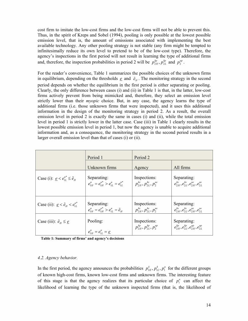
For the reader’s convenience, Table 1 summarizes the possible choices of the unknown firms in equilibrium, depending on the thresholds e and He . The monitoring strategy in the second period depends on whether the equilibrium in the first period is either separating or pooling. Clearly, the only difference between cases (i) and (ii) in Table 1 is that, in the latter, low-cost firms actively prevent from being mimicked and, therefore, they select an emission level strictly lower than their myopic choice. But, in any case, the agency learns the type of additional firms (i.e. those unknown firms that were inspected), and it uses this additional information in the design of the monitoring strategy in period 2. As a result, the overall emission level in period 2 is exactly the same in cases (i) and (ii), while the total emission level in period 1 is strictly lower in the latter case. Case (iii) in Table 1 clearly results in the lowest possible emission level in period 1, but now the agency is unable to acquire additional information and, as a consequence, the monitoring strategy in the second period results in a larger overall emission level than that of cases (i) or (ii).

Period 1 Period 2

Unknown firms Agency All firms

Case (i): *1uL He e e< ≤

Separating: * *

1 1 1 1u u u uH H L Le e e e= > =

Inspections: 2 2 2, ,ks ks us

H Lp p p Separating:

2 2 2 2, , ,ks ks us usH L H Le e e e

Case (ii): *1u

H Le e e< < Separating: *

1 1 1u u uH H L He e e e= > =

Inspections: 2 2 2, ,ks ks us

H Lp p p Separating:

2 2 2 2, , ,ks ks us usH L H Le e e e

Case (iii): He e≤ Pooling:

1 1u uH Le e e= =

Inspections: 2 2 2, ,kp kp up

H Lp p p Separating:

2 2 2 2, , ,kp kp up upH L H Le e e e

Table 1: Summary of firms’ and agency’s decisions

4.2. Agency behavior.

In the first period, the agency announces the probabilities 1 1 1, ,k k uH Lp p p for the different groups

of known high-cost firms, known low-cost firms and unknown firms. The interesting feature of this stage is that the agency realizes that its particular choice of 1

up can affect the likelihood of learning the type of the unknown inspected firms (that is, the likelihood of

15

obtaining a separating equilibrium among the subset of unknown firms). The agency has this option to influence firms’ compliance behavior since the choice of 1

up affects the level of the threshold He (defined in expression (4)) as well as the level of the myopic choice *

1uLe (defined

in Lemma 1), and this is crucial in determining the type of equilibrium that may arise, as shown in Table 1 above.

In the following, we present the relationship between the threshold He and the myopic choice of an unknown low-cost type *

1uLe for each level of the probability 1

up .

Lemma 2. The threshold level He is strictly decreasing and convex in 1up . Also, there exists a

unique ( )1 0,uHp p∈ such that ( ) ( )*

1 1 1u u u

H Le p e p> for all 1 1u up p< , ( ) ( )*

1 1 1u u u

H Le p e p= and

( ) ( )*1 1 1u u u

H Le p e p< for all 1 1u up p> .

In Figure 2, we provide an illustration of the result presented in Lemma 2. This lemma is crucial in determining the optimal choices (marked with bold lines in the figure) of the two types of unknown firms for the different values of the inspection probability 1

up . The figure presents the myopic responses of the two firm types (that is, * *

1 1,u uH Le e , as obtained in Lemma

1) as well as the threshold level He as functions of 1up . Each function *

1uie starts at 0

ie when

1 0up = and is strictly decreasing in 1up until the inspection probability achieves the threshold

probability ip defined in equation (1). Then, for 1u

ip p> , the optimal choice of a type i firm is to comply with the standard, that is, *

1uie e= . The function He coincides with *

1uHe when

1 0up = at the level 0He . When 1 0up = , unknown firms are not inspected at all and the agency

does not learn the type of any of these firms. Thus, unknown high-cost firms cannot gain anything by trying to reduce their emission level below their myopic cost minimization level. On the other hand, it is easy to see that the threshold level He is strictly below the standard e when 1

uHp p= . After all, when 1

uHp p= , the high-cost firm’s myopic choice is precisely to

comply with the standard; mimicking would then imply an additional effort by the firm allowing its emission level to fall below the standard.

16

CASE (i) CASE (ii) CASE (iii)

High-cost type behavior

Low-cost type behavior

1

up 1

up

He

Lp Hp1

ˆ up

*1uHe

*1uLe

oLe

e

oHe

e

Figure 2: Unknown firms’ behavior

Since He is strictly decreasing and convex in 1up , we have that the function He crosses only

once with the function *1uLe (at the probability 1

up ). Therefore, we can replicate the three cases of Table 1 depending on the probability 1

up of inspecting the unknown firms being below or above the threshold level 1

up .20

Thus, case (i) of Table 1 corresponds to the situation where 1 1u up p≤ . For a sufficiently low

inspection probability, the expected gain for an unknown high-cost firm from pretending to be a low-cost type is rather small. Therefore, the lowest emission level that the firm is willing to implement is not sufficient to successfully imitate a low-cost firm. In this case, the outcome is a separating equilibrium in which the threat of mimicking is absent and each firm chooses its myopic emission level *

1uie (see bold lines in case (i) of Figure 2).

We obtain case (ii) of Table 1 for intermediate values of the inspection probability, that is, when 1 1 1ˆu u up p p< ≤ , where 1ˆ up is such that ( )1ˆ u

He p e= . Compared to case (i), the gains of mimicking increase since an unknown high-cost firm is now more frequently inspected in period one. Therefore, low-cost firms have to actively deter mimicking by high-cost firms. As a result, high-cost firms select their myopic response *

1uHe while low-cost firms select the level

He (see bold lines in case (ii) of Figure 2). Again, we obtain a separating equilibrium, but with a credible threat of mimicking that may lead low-cost firms to over-comply with the regulation (in Figure 2, this happens from 1

up onwards).

20 The crossing point between He and *

1uLe can be at probability 1

up between Lp and Hp , as illustrated in

Figure 2, or at a probability strictly below L

p , although this does not affect the nature of our results.

17

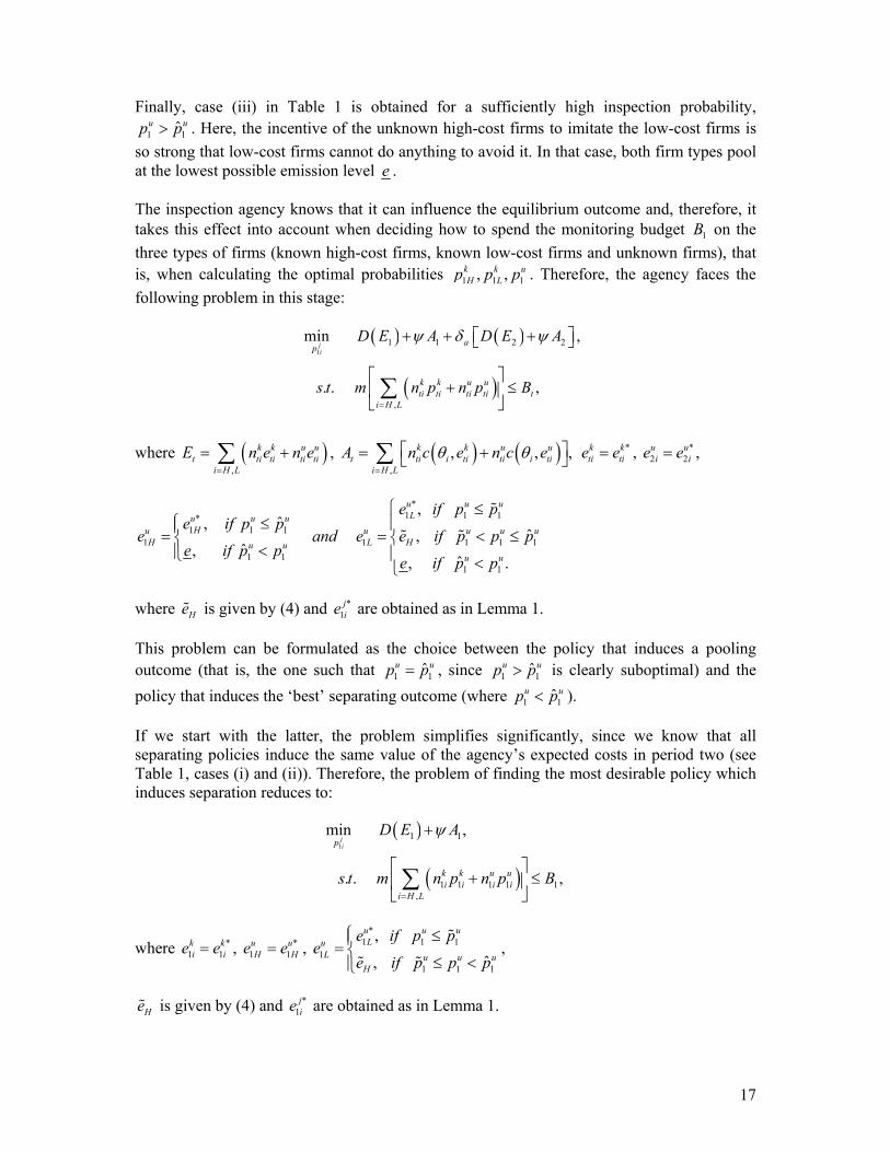
Finally, case (iii) in Table 1 is obtained for a sufficiently high inspection probability, 1 1ˆu up p> . Here, the incentive of the unknown high-cost firms to imitate the low-cost firms is

so strong that low-cost firms cannot do anything to avoid it. In that case, both firm types pool at the lowest possible emission level e .

The inspection agency knows that it can influence the equilibrium outcome and, therefore, it takes this effect into account when deciding how to spend the monitoring budget 1B on the three types of firms (known high-cost firms, known low-cost firms and unknown firms), that is, when calculating the optimal probabilities 1 1 1, ,k k u

H Lp p p . Therefore, the agency faces the following problem in this stage:

( ) ( )

( )

11 1 2 2

,

min ,

. . ,

ji

ap

k k u uti ti ti ti t

i H L

D E A D E A

s t m n p n p B

ψ δ ψ

=

+ + +⎡ ⎤⎣ ⎦

⎡ ⎤+ ≤⎢ ⎥

⎣ ⎦∑

where ( ),

k k u ut ti ti ti ti

i H LE n e n e

=

= +∑ , ( ) ( ),

, , ,k k u ut ti i ti ti i ti

i H LA n c e n c eθ θ

=

⎡ ⎤= +⎣ ⎦∑ *k kti tie e= , *

2 2u ui ie e= ,

*1 1 1*

1 1 11 1 1 1 1

1 11 1

,ˆ,

ˆ,ˆ,

ˆ, .

u u uLu u u

Hu u u u uH L Hu u

u u

e if p pe if p p

e and e e if p p pe if p p

e if p p

⎧ ≤⎧ ≤ ⎪⎪= = < ≤⎨ ⎨

<⎪ ⎪⎩ <⎩

where He is given by (4) and *1jie are obtained as in Lemma 1.

This problem can be formulated as the choice between the policy that induces a pooling outcome (that is, the one such that 1 1ˆu up p= , since 1 1ˆu up p> is clearly suboptimal) and the policy that induces the ‘best’ separating outcome (where 1 1ˆu up p< ).

If we start with the latter, the problem simplifies significantly, since we know that all separating policies induce the same value of the agency’s expected costs in period two (see Table 1, cases (i) and (ii)). Therefore, the problem of finding the most desirable policy which induces separation reduces to:

( )

( )1

1 1

1 1 1 1 1,

min ,

. . ,

jip

k k u ui i i i

i H L

D E A

s t m n p n p B

ψ

=

+

⎡ ⎤+ ≤⎢ ⎥

⎣ ⎦∑

where *1 1k ki ie e= , *

1 1u uH He e= ,

*1 1 1

11 1 1

,ˆ,

u u uLu

L u u uH

e if p pe

e if p p p

⎧ ≤⎪= ⎨≤ <⎪⎩

,

He is given by (4) and *1jie are obtained as in Lemma 1.

18

We can now divide the problem into two parts depending on whether the optimal probability for the unknown firms, 1

up , is larger or lower than 1up . For this reason, we measure at the

threshold level 1up the marginal impact on the agency’s social cost evaluation of spending an

additional monetary unit in inspecting each of the groups. If the marginal impact of spending an additional monetary unit in inspecting unknown firms is smaller at that level 1

up (in absolute terms) than that of spending an additional monetary unit in inspecting previously known firms, then the optimal policy is such that 1 1

u up p≤ ; that is, it lies in case (i) of Figure 2. Otherwise, the optimal policy is such that 1 1

u up p> and case (ii) of Figure 2 is implemented

by the agency. This threshold policy ( )1 1 1, ,k k uH Lp p p is trivially obtained by calculating the

amount of money needed to inspect the unknown firms with probability 1up and then

allocating the remaining budget efficiently between the groups of known high-cost and low-cost firms, along the lines of Proposition 1. That is, ( )1 1 1, ,k k u

H Lp p p is obtained from the following conditions:

( ) ( )

( )

( )( ) ( )( )

( ) ( )

*1 1 1

1 1 1 1 1 1,

1 11 1

1 1

1 1 1 1

;

;

' ' ;

, 0; , 0.

u u uH L

k k u u ui i H L

i H L

k kk kH LH Lk k

H L

k k u ue i i H e L L

e p e p

B m n p n n p

e eD E p f D E p fp p

c e p f c e p f

ψ ψ

θ θ

=

=

⎛ ⎞= + +⎜ ⎟

⎝ ⎠

∂ ∂− = −

∂ ∂

+ = + =

∑

where E is the overall emission level induced by the threshold policy ( )1 1 1, ,k k uH Lp p p .

We are now ready to characterize the optimal policy that induces separation in the first regulatory period. Also remember that aE stands for the agency’s most preferred aggregate emission level.

Proposition 2. Assume that aLe e≤ . Then, the (interior) optimal inspection probabilities

( )* * *1 1 1, ,k k u

H Lp p p which induce separation in the first regulatory period are obtained as follows:

(i) If ( ) ( )1 1 11 1

,1 1 1 1

' 'k u u

k ui i ii k u u u

i H Li H L

e n eD E p f D E p fp n n p

ψ ψ=

⎡ ⎤∂ ∂⎡ ⎤ ⎡ ⎤− ≤ − ⎢ ⎥⎣ ⎦ ⎣ ⎦∂ + ∂⎣ ⎦∑ , then:

a. If ( )

1

' aD EmN B

fψ≤ , then

( )* * *1 1 1

' ak k uH L

D Ep p p

fψ= = = .

19

b. If ( )

1

' aD EmN B

fψ> , then:

( ) ( )* *1 1 11 1

,1 1 1 1

' 'k u u

k ui i ii k u u u

i H Li H L i

e n eD E p f D E p fp n n p

ψ ψ=

⎡ ⎤∂ ∂⎡ ⎤ ⎡ ⎤− = − ⎢ ⎥⎣ ⎦ ⎣ ⎦∂ + ∂⎣ ⎦∑ , where

( )( )* *1 1 1 1 1 1

,

k k u u ui i H L

i H Lm n p n n p B

=

⎡ ⎤+ + =⎢ ⎥

⎣ ⎦∑ , ( ) *

1 1, 0k ke i i ic e p fθ + = and

( ) *1 1, 0u u

e i ic e p fθ + = .

(ii) If ( ) ( )1 1 11 1

,1 1 1 1

' 'k u u

k ui i ii k u u u

i H Li H L

e n eD E p f D E p fp n n p

ψ ψ=

⎡ ⎤∂ ∂⎡ ⎤ ⎡ ⎤− > − ⎢ ⎥⎣ ⎦ ⎣ ⎦∂ + ∂⎣ ⎦∑ , then:

( ) ( )

( ) ( )( )

* *1 1 11 1

1 1 1 1

*11

1 1 1

' '

' , ,

k u uk ui H Hi k u u u

i H L

uuL H

e H Hu u uH L

e n eD E p f D E p fp n n p

n eD E c e pn n p

ψ ψ

ψ θ

∂ ∂⎡ ⎤ ⎡ ⎤− = − +⎣ ⎦ ⎣ ⎦∂ + ∂

∂⎡ ⎤+⎣ ⎦+ ∂

where ( )( )* *1 1 1 1 1 1

,

k k u u ui i H L

i H Lm n p n n p B

=

⎡ ⎤+ + =⎢ ⎥

⎣ ⎦∑ , ( ) *

1 1, 0k ke i i ic e p fθ + = ,

( ) *1 1, 0u u

e H Hc e p fθ + = and ( )*1 1u uL He e p= is given by (4).

Therefore, the optimal inspection policy which induces separation is located in case (i) of Figure 2, when the marginal impact of spending an additional monetary unit in inspecting unknown firms at that level 1

up is no larger (in absolute terms) than that of spending an additional monetary unit in inspecting previously known firms. There, the optimal inspection strategy is the same as that presented in Proposition 1, since both types of unknown firms select their myopic strategies (see Lemma 1). If, however, the marginal impact of inspecting unknown firms at that level 1

up is larger (in absolute terms) than that of inspecting the known firms, then the optimal inspection strategy which induces separation is located in case (ii) of Figure 2. There, the optimality condition satisfies the property that the last monetary unit spent in each firms group has the same marginal effect on the environmental damages and the weighted abatement costs, but the agency now takes into account that the unknown low-cost firms will actively prevent being mimicked by the high-cost firms. As a result, the agency has to consider that the marginal impact of inspecting unknown firms is larger than when low-cost firms do not need to prevent mimicking.

The last step in finding the optimal inspection strategy in the first period is to compare the overall discounted social costs of the optimal policy which induces separation (characterized in Proposition 2) with those of the policy which induces pooling. This pooling policy ( )1 1 1ˆ ˆ ˆ, ,k k u

H Lp p p is trivially obtained by means of the following conditions:

20

( )

( )

( )( ) ( )( )( )

1

1 1 1 1 1 1,

1 11 1

1 1

1 1

ˆ ;

ˆ ˆ ;

ˆ ˆˆ ˆ' ' ;

ˆ, 0;

uH

k k u u ui i H L

i H L

k kk kH LH Lk k

H L

k ke i i i

e p e

B m n p n n p

e eD E p f D E p fp p

c e p f

ψ ψ

θ

=

=

⎛ ⎞= + +⎜ ⎟

⎝ ⎠

∂ ∂− = −

∂ ∂

+ =

∑

where E is the overall emission level induced by the pooling policy ( )1 1 1ˆ ˆ ˆ, ,k k uH Lp p p .

All this reasoning leads us to a unique perfect Bayesian equilibrium that can induce either separating or pooling behavior, depending on which one induces the lowest possible weighted social costs. Therefore, the equilibrium is unique, but it can be located in any of the three regions of Figure 2. It can imply either separating or pooling behavior by unknown firms. From a strict deterrence point of view (that is, when ψ is sufficiently small), it is clear that case (ii) in Table 1 dominates case (i), since the overall emission level in case (ii) is smaller. However, the additional abatement costs spent by low-cost firms to actively prevent imitation can be very large and, consequently, case (i) might then be preferred over case (ii) when ψ is large enough. Also, the pooling outcome (case (iii) of Table 1) can be very attractive in terms of deterrence (especially if the discount rate aδ is sufficiently low); however, abatement costs in this case are the largest, which is surely detrimental from a social cost viewpoint.

When ψ is close to 1, the inspection agency’s objective function takes the social costs associated with the standard into account and, therefore, no intervention into the agency’s decision process is needed. However, when ψ is small, the agency strongly favors deterrence and aims at reducing breaches of the standard regardless of the costs to firms. Clearly, the lower ψ , the stronger the (unknown) high-cost firms’ incentives to mimic low-cost firms and, therefore, the more likely the pooling outcome at the lowest possible emission level arises.

V. MODEL IMPLICATIONS

In this section we present some implications of our results as well as some directions for empirical research.

From the analysis of our signaling game we find that the agency can try to influence firms’ strategic behavior by selecting an appropriate inspection strategy in the first period within budgetary limits. We show that the agency will devote more enforcement resources in the second period to auditing the known high-cost firms than the known low-cost firms (whose reactions to a change in the inspection probability are larger). In principle, this targeting strategy can be detrimental for high-cost firms, but beneficial for low-cost firms. Therefore, high-cost firms may have an incentive to avoid this situation by trying to mimic the low-cost firms; although low-cost firms may try to avoid being mimicked. However, if firms’ abatement costs are sufficiently large, intervention into the agency’s decision process might be socially desirable since mimicking and avoidance behavior is socially costly. Several

21

options can be considered for this intervention. Firstly, it might be possible to influence the form of the agency’s objective function by increasing the weight attached to firms’ compliance costs. This could be done by changing the agency’s mission statement combined with independent, external evaluation of the agency’s performance. Secondly, the regulator might consider ways to alleviate the information asymmetry, such as making public reports by firms on their emission levels mandatory. Further, the regulator might use the budget allocated to the agency to influence the inspection policy selected. A small budget will make the deterrent agency select an inspection policy leading to a myopic separating equilibrium, ceteris paribus, while a large budget will lead to a pooling equilibrium, ceteris paribus. Finally, the regulator might also allow exceptions to the legal standard if these exceptions are sufficiently motivated by firms, for instance, by referring to excessive compliance costs. A licensing system for individual firms is a typical example of this type of regulatory practice.

In order to test the model results in practice, attention should be shifted to industries where mimicking and/or avoidance of mimicking is more likely to occur. As we mentioned in the introduction, key assumptions in our model are the continuous pollution decisions and also the fact that inspections are based on pollution records. Thus, our model can be more appropriate in industries where future inspections are based on past emissions levels (i.e., past emissions as an explanatory variable for future monitoring): see, for instance, the evidence cited in the introduction for the US pulp and paper, chemical and steel industries, the Canadian petroleum storage or US hazardous waste regulations.21 Another important assumption is that regulators do not have perfect information about the specific abatement cost characteristics of the regulated firms, and regulators acquire that information interacting with polluting firms through time. Thus, it seems plausible that evidence of mimicking and/or over-compliance might be found in settings where regulations are recently introduced, polluters are heterogeneous with respect to abatement possibilities, involve uniform standards (since there is no justification to discriminate among polluters due to lack of information) and relate to a sufficiently large number of installations.

Two prominent examples of new regulations which are (being) established and which are relevant for some of the industrial sectors mentioned above are:

1) The new Clean Air Act standards for particulate matter, mercury and carbon oxide emissions by industrial boilers and incinerators announced by the EPA (EPA 2011). These uniform emission standards for boilers depend on the age and size of the boiler and are independent of the industrial sector. According to Fisher International Inc (2010), the new standards would threaten some 16000 jobs in the US pulp and paper industry.

2) The proposals to reform the Toxic Substance Control Act (TSCA) 1976 in 2011 are potentially interesting. Several proposals were already presented to the US Senate and House in 2010 (but they were not put to vote yet). TSCA is relevant for several US industries, including the chemical industry.

21 Also, firms that are thought to have a high risk of causing considerable environmental damage are inspected more frequently. One of the parameters used to categorize firms in risk classes is the amount of emissions produced. An overview of possible criteria (including emissions and scale of facility) for environmental risk assessment is provided by the IMPEL report ‘Doing the right things II’ a guidance document for environmental inspectorates in the EU member states (consult IMPEL 2008, http://impel.eu/wp‐content/uploads/2010/02/2007‐11‐dtrt2‐step‐by‐step‐guidance‐book‐FINAL‐REPORT.pdf). 

22

In our opinion, future analysis of the monitoring activities of the US EPA and the emission levels in the regulated industries might thus provide a fruitful ground for empirical testing of our model results.

VI. CONCLUSIONS

This paper shows that incorporating learning into regulatory enforcement has implications for the agency and the firms’ strategies, as well as for social costs. We assume that the regulatory agency has the possibility to learn about the true type of previously unknown firms by inspecting them, but only if it finds subgroups of firms performing differently. This type of learning is used afterwards to target known types in the subsequent regulatory period. Since we assume that the type of some firms is already known by the agency at the beginning of the game, we also include the trade-off between controlling emissions levels of firms of known type and learning the type of additional firms. This type of learning induces an interesting signaling game which is new in the enforcement literature, and which may lead to either separating or pooling behavior.

The signaling game presented clearly influences the firms’ emission levels. In any case, the incentives of low-cost firms to avoid mimicking result in a lower amount of global emissions in the first period. On the one hand, the high-cost types may try to reduce emissions in the first period to avoid future tighter monitoring. On the other hand, the low-cost types may try to reduce emissions as well, in order to differentiate themselves from the high-cost types and thus prevent being pooled. Sometimes they might even avoid being imitated by doing better than the emission standard in the first period (i.e. by over-complying).

Finally, it is interesting to note that as long as the number of regulatory stages increases, the pooling scenario becomes less likely. Indeed, there would be more periods where high-cost firms incur in imitation costs, while the benefits of mimicking would only be reached in the last period. This observation also implies that a reversal in strategy (from pooling to separating or from separating to pooling) is not likely either. As a consequence, in a game with a sufficiently large number of regulatory periods, the agency is always able to learn the firms’ true type through inspections, since high-cost firms never pose as low-cost firms. This infinitely repeated game converges to a steady-state equilibrium, which involves a cost efficient allocation of the available funds. This means that agency’s resources are used where they cause the greatest reduction in the level of the externality. However, an infinitely repeated game is not a realistic representation of regulatory practices since regulations are repeatedly modified and replaced: for example, 27 new environmental legislations came into force in 2010 in England alone (consult www.netregs.gov.uk).

23

APPENDIX

Proof of Lemma 1. The first order conditions of this optimization problem are:22

( )2 2

2 2

, 0,

0, 0, 0,

j je i i i

j ji i

c e p f

e e e e

θ λ

λ λ

+ − =

⎡ ⎤≥ − ≥ − =⎣ ⎦

where 0λ ≥ is the Kuhn-Tucker multiplier associated to the inequality restriction. Easily combining these conditions, we obtain the desired result.

Proof of Proposition 1. The optimality conditions of this problem are the following:

( )( )

( )( ) ( )

22

2

2 22 2 2 2 2

2 2

' , 0, , ;

' , 0, , ;

kk i

e i i ki

u uu u u u uH L

e i i H L H Lu uH L

eD c e m i H Lp

e eD c e n n m n n i H Lp p

ψ θ α

ψ θ α

∂+ + = =

∂

⎛ ⎞∂ ∂+ + + + = =⎜ ⎟∂ ∂⎝ ⎠

where 0α ≥ is the Kuhn-Tucker multiplier associated with the budgetary restriction.

First, if the budgetary restriction is not binding ( 0α = ), these two conditions reduce to:

( ) ( )2 2' , ' ,k ue i i e i iD c e D c eψ θ ψ θ+ = + ,

which lead to the uniform monitoring policy:

( )

2

', , , , .

aji

D Ep i H L j k u

fψ= = =

This solution is valid only if ( )

2

' aD EmN B

fψ≤ . Otherwise, we have 0α ≥ , and the two above

conditions reduce to:

( )( ) ( )( )2 2 22 2

,2 2 2 2

' , ' , , ,k u u

k ui i ie i i e i ik u u u

i H Li H L i

e n eD c e D c e i H Lp n n p

ψ θ ψ θ=

⎛ ⎞∂ ∂+ = + =⎜ ⎟∂ + ∂⎝ ⎠

∑ ,

where ( )2 2, j je i i ic e p fθ = and ( )2 2 2 2 2

,

k k u ui i i i

i H Lm n p n p B

=

⎡ ⎤+ =⎢ ⎥

⎣ ⎦∑ .

Proof of Lemma 2. Differentiating expression (4) with respect to He and 1up , we have:

( ) ( ) ( )

( )

*1 2 2

1 1

, ,u ks usH H f H H HH

u ue H

f e e p pep c e p f

δ θ θ⎡ ⎤− − −∂ ⎣ ⎦= −∂ +

.

Using Lemma 1, expression (1), and defining ( ) ( )2 2, ,ks usH H Hh p pθ θ= − , this expression

can be easily reduced as follows: 22 Given the assumptions of our model, these are necessary and sufficient conditions for an optimum. The same applies for the remaining optimization problems in the paper.

24

( )1

*1 1 1

0u

fH Hu u u

ee H H

he ep p c e e

δ∂ ∂= + <

∂ ∂ −, (5)

since 1

1

0uHu

ep

∂<

∂, *

1 0uH He e− < and 0h > , since 2 2

ks usHp p> .

To prove the convexity, we derivate the above expression with respect to 1up to obtain:

( ) ( )

*1

21 1

2 2*1 1

0

uH H

f u uH

u uee H H

e ehp pe

p c e e

δ⎛ ⎞∂ ∂

−⎜ ⎟∂ ∂∂ ⎝ ⎠= − >∂ −

,

since *

1

1 1

uH Hu u

e ep p∂ ∂

<∂ ∂

, see (5).

The function He is strictly decreasing and convex in 1up . Therefore, it is sufficient to prove

that the functions He and *1uLe cross to be sure that they cross only once. To show this, it is

enough to prove that *1u

H Le e> when 1 0up = and *1u

H Le e< when 1u

Hp p= . On the one hand, * 0

1u

H H He e e= = when 1 0up = (the unknown firms do not gain anything by trying to reduce their emissions since they are not inspected) and He e< when 1

uHp p= . On the other hand,

* 0 01uL L He e e= < when 1 0up = and *

1uLe e= when 1

uHp p= , since L Hp p= . As a result, we obtain

*1u

H He e> when 1 0up = and *1u

H He e< when 1u

Hp p= . By continuity, there necessarily exists

( )1 0,uHp p∈ such that both functions He and *

1uHe cross, as desired.

Proof of Proposition 2. To prove part (i), consider the case where 1 1u up p≤ . The optimality

conditions of this (constrained) problem are the following:

( )( )

( )( ) ( )

11

1

1 11 1 1 1 1

1 1

' , 0, , ;

' , 0, , ;

kk i

e i i ki

u uu u u u uH L

e i i H L H Lu u

eD c e m i H Lp

e eD c e n n m n n i H Lp p

ψ θ α

ψ θ α δ

∂+ + = =

∂

⎛ ⎞∂ ∂+ + + + + = =⎜ ⎟∂ ∂⎝ ⎠

where 0α ≥ , 0δ ≥ are the Kuhn-Tucker multipliers associated, respectively, with the budgetary constraint and the probability restriction 1 1

u up p≤ . If 0δ = , the result is identical to that of Proposition 1, provided that the resulting inspection probability for the unknown firms is 1 1

u up p< . Otherwise, 0δ ≥ and 1 1u up p= , but then, combining the above two conditions, we

need that the following condition evaluated at 1 1u up p= holds:

( )( ) ( )( )1 1 11 1 1 1

1 1 1

' , ' ,u u k

u u u kH L He i i H L e i iu u k

H

e e eD c e n n D c ep p p

ψ θ ψ θ⎛ ⎞∂ ∂ ∂

+ + ≥ +⎜ ⎟∂ ∂ ∂⎝ ⎠.

If this condition does not hold, we have to look at the next range of probabilities, which lead as to case (ii) of the proposition. Now, the two optimality conditions of this new (constrained) problem become:

25

( )( )

( )( ) ( )

11

1

11 1 1 1 1

1 1

' , 0, , ;

' , 0, , ;

kk i

e i i ki

uu u u u uH H

e i i H L H Lu u

eD c e m i H Lp

e eD c e n n m n n i H Lp p

ψ θ α

ψ θ α β

∂+ + = =

∂

⎛ ⎞∂ ∂+ + + + + = =⎜ ⎟∂ ∂⎝ ⎠

where 0α ≥ , 0β ≥ are the Kuhn-Tucker multipliers associated, respectively, with the budgetary constraint and the probability restriction 1 1 .u up p≤ Combining both conditions for

0β = , we obtain the desired result.

26

REFERENCES

1. Arora, S., Gangopadhyay, S., 1995. Toward a theoretical model of voluntary overcompliance. Journal of Economic Behavior and Organization 28, 289-309.

2. Bagnoli, M., Watts, S.G., 2003. Selling to socially responsible consumers: competition and the private provision of public goods. Journal of Economics and Management Strategy 12, 419–445.

3. Bose, P., 1995. Regulatory errors, optimal fines and the level of compliance. Journal of Public Economics 56, 475-484.

4. Cho, I., Kreps, D.M., 1987. Signaling games and stable equilibria. The Quarterly Journal of Economics 102, 179-221.

5. Cohen, M.A., 1987. Optimal enforcement strategy to prevent oil spills: an application of a principal-agent model with moral hazard. Journal of Law and Economics 30: 23-51.

6. Costello, C., Karp, L., 2004. Dynamic taxes and quotas with learning. Journal of Economic Dynamics & Control 28, 1661-1680.

7. Decker, C.S., 2005. Do regulators respond to voluntary pollution control efforts? A count data analysis. Contemporary Economic Policy 23, 180-194.

8. Decker, C.S., 2006. Implementing environmental regulation: an inter-industry analysis. Eastern Economic Journal 32, No.1.

9. Decker, C.S., Pope, C.R., 2005. Adherence to environmental law: The strategic complementarities of compliance decisions. Quarterly Review of Economics and Finance 45, 641-661.

10. Denicolò, V., 2008. A signaling model of environmental overcompliance. Journal of Economic Behavior & Organization 68, 293-303.

11. Eckert, H., 2004. Inspections, warnings, and compliance: the case of petroleum storage regulation. Journal of Environmental Economics and Management 47, 232-259

12. EPA, 2011. EPA Establishes Clean Air Act Standards for Boilers and Incinerators. Press release 02/23/2011

13. Firestone, J., 2003. Enforcement of pollution laws and regulations: An analysis of forum choice. Harvard Environmental Law Review 27, 105-176.

14. Fisher International Inc, 2010. Economic Impact of Pending Air Regulations on the U.S. Pulp and Paper Industry

15. Friesen, L., 2003. Targeting enforcment to improve compliance with Environmental regulations. Journal of Environmental Economics and Management 46, 72-85.

16. Fudenberg, D., Tirole, J., 1991a. Perfect Bayesian and sequential equilibrium. Journal of Economic Theory 53, 236-260.

27

17. Fudenberg, D., Tirole, J., 1991b. Game Theory. MIT Press, Cambridge.

18. Gray, W.B., Deily, M.E., 1996. Compliance and enforcement: Air pollution regulation in the US steel industry. Journal of Environmental Economics and Management 31, 96-111.

19. Grossman, S.J., 1981. The role of warranties and private disclosure about product quality. Journal of Law and Economics 24, 461-483.

20. Harford, J.D., Harrington, W., 1991. A reconsideration of enforcement leverage when penalties are restricted. Journal of Public Economics 45, 391-395.

21. Harrington, W., 1988. Enforcement leverage when penalties are restricted. Journal of Public Economics 37, 29-53.

22. Heyes, A., Kapur, S., 2009. Enforcement missions: Targets vs. budgets. Journal of Environmental Economics and Management 58, 129-140.

23. Keeler, A., 1995. Regulatory objectives and enforcement behavior. Environmental and Resource Economics 6, 73-85.

24. Kreps, D.M., Sobel, J., 1994. Signaling, in Aumann, R.J., Hart, S. (Eds.), Handbook of Game Theory, Vol.2. Elsevier, Amsterdam.

25. Lee, D.R 1983. Monitoring and Budget Maximization in the Control of Pollution. Economic Inquiry, 21(4), 565-575

26. Lyon, T.P., Maxwell, J.W., 2003. Self-regulation, taxation and public voluntary environmental agreements. Journal of Public Economics 87, 1453–1486.

27. Lyon, T.P., Maxwell, J.W., 2004. Corporate Environmentalism and Public Policy. Cambridge University Press, Cambridge.

28. Makowsky, M D., Stratmann, T., 2009. Political Economy at Any Speed: What Determines Traffic Citations?. The American Economic Review 99(1), 509-527.

29. Maxwell, J.W., Lyon, T.P., Hackett, S.C., 2000. Self-regulation and social welfare: the political economy of corporate environmentalism. Journal of Law and Economics 43, 583–617.

30. Mookherjee D., Png, I.P.L., 1994. Marginal deterrence in enforcement of law. The Journal of Political Economy 102(5), 1039-1066

31. Mookherjee, D., Png, I.P.L., 1995. Corruptible Law Enforcers: How Should They Be Compensated? The Economic Journal 105( 428), 145-159

32. Nadeau, L.W., 1997. EPA effectiveness at reducing the duration of plant-level noncompliance. Journal of Environmental Economics and Management 34, 54-78.

33. Nyborg, K., Telle, K., 2004. The role of warnings in regulation: Keeping control with less punishment. Journal of Public Economics 88(12), 2801-2816.

28

34. Polinsky, A.M., Shavell, S., 1979. The optimal tradeoff between the probability and magnitude of fines. American Economic Review 69(5): 880-891.

35. Polinsky, A.M., Shavell, S., 1991. A note on optimal fines when wealth varies among individuals. American Economic Review 81(3), 618-621.

36. Polinsky, A.M., Shavell, S., 1992. Enforcement costs and the optimal magnitude and probability of fines. The Journal of Law and Economics 35, 133-148.

37. Polinsky, A.M., Shavell, S., 2000. The economic theory of public enforcement of law. Journal of Economic Literature 37, 45-76.

38. Raymond, M., 1999. Enforcement leverage when penalties are restricted: A reconsideration under asymmetric information. Journal of Public Economics 73, 289-295.

39. Reinganum, J.F., Wilde, L.L., 1986. Settlement, litigation and the allocation of litigation costs. The RAND Journal of Economics 17, 557-566.

40. Riley, J.G., 1979. Informational equilibrium. Econometrica 47, 331-359.

41. Robinson, E. J. Z.;, Lokina, R. B., (2009). Spatial aspects of forest management and non-timber forest product extraction in Tanzania. Environment for Development Discussion Paper - Resources for the Future No. 09-07

42. Rothschild, M., Stiglitz, J.E.,1976. Equilibrium in competitive insurance markets: An essay on the economics of imperfect information. Quarterly Journal of Economics 80, 629-649.

43. Rousseau, S., 2007. Timing of environmental inspections: Survival of the compliant. Journal of Regulatory Economics 32(1), 17-36.

44. Rousseau, S., 2009. The use of warnings in the presence of errors. International Review of Law and Economics 29, 191-201.

45. Shavell, S., 1987. The optimal use of nonmonetary sanctions as a deterrent. American Economic Review 77(4), 584-592.

46. Shavell, S., 1992. A note on marginal deterrence. International Review of Law and Economics 12, 133-49.

47. Shimshack, J.P., Ward, M.B., 2008. Enforcement and overcompliance. Journal of Environmental Economics and Management 55, 90–105.

48. Sobel, J., 1989. An analysis of discovery rules. Law and Contemporary Problems 52, 133-159.

49. Spence, M., 1973. Job market signaling. Quarterly Journal of Economics 87, 355-374.

50. Wu, J., Wirkkala, T.M., 2009. Firms’ motivations for environmental overcompliance. Review of Law and Economics 5, art. 17.