cartographica user's guide - macgis.com · data with a specific datum, might find that their...

Cartographica User's Guide

Version 1.4.6

Cartographica User's Guide: Version 1.4.6Publication date December 3, 2015Copyright © 2010-2015 ClueTrust (GBP Software, LLC)

ClueTrust, the ClueTrust lightbulb logo, Cartographica, and the Cartographica logo are registered trademarks of GBP Software, LLC.

Table of Contents1. Introduction .... . . . . . . . . . . . . . . . . . . . . . . . . . . . . . . . . . . . . . . . . . . . . . . . . . . . . . . . . . . . . . . . . . . . . . . . . . . . . . . . . . . . . . . . . . . . . . . . . . . . . . . . . . . . . . . . . 1

1.1. About Cartographica .... . . . . . . . . . . . . . . . . . . . . . . . . . . . . . . . . . . . . . . . . . . . . . . . . . . . . . . . . . . . . . . . . . . . . . . . . . . . . . . . . . . . . . . . . . . 11.2. Projections, Coordinate Systems, and Datum ..... . . . . . . . . . . . . . . . . . . . . . . . . . . . . . . . . . . . . . . . . . . . . . . . . . . . . . . . . . . 11.3. Features ... . . . . . . . . . . . . . . . . . . . . . . . . . . . . . . . . . . . . . . . . . . . . . . . . . . . . . . . . . . . . . . . . . . . . . . . . . . . . . . . . . . . . . . . . . . . . . . . . . . . . . . . . . . . . . 11.4. Layers ... . . . . . . . . . . . . . . . . . . . . . . . . . . . . . . . . . . . . . . . . . . . . . . . . . . . . . . . . . . . . . . . . . . . . . . . . . . . . . . . . . . . . . . . . . . . . . . . . . . . . . . . . . . . . . . . 2

2. Getting Started with Cartographica .... . . . . . . . . . . . . . . . . . . . . . . . . . . . . . . . . . . . . . . . . . . . . . . . . . . . . . . . . . . . . . . . . . . . . . . . . . . . . . . . . . . 32.1. Installing Cartographica .... . . . . . . . . . . . . . . . . . . . . . . . . . . . . . . . . . . . . . . . . . . . . . . . . . . . . . . . . . . . . . . . . . . . . . . . . . . . . . . . . . . . . . . 32.2. Updating Cartographica .... . . . . . . . . . . . . . . . . . . . . . . . . . . . . . . . . . . . . . . . . . . . . . . . . . . . . . . . . . . . . . . . . . . . . . . . . . . . . . . . . . . . . . . 42.3. Interface Overview .... . . . . . . . . . . . . . . . . . . . . . . . . . . . . . . . . . . . . . . . . . . . . . . . . . . . . . . . . . . . . . . . . . . . . . . . . . . . . . . . . . . . . . . . . . . . . . 5

2.3.1. Utility Windows .... . . . . . . . . . . . . . . . . . . . . . . . . . . . . . . . . . . . . . . . . . . . . . . . . . . . . . . . . . . . . . . . . . . . . . . . . . . . . . . . . . . . . . . 72.3.2. The Uber Browser ... . . . . . . . . . . . . . . . . . . . . . . . . . . . . . . . . . . . . . . . . . . . . . . . . . . . . . . . . . . . . . . . . . . . . . . . . . . . . . . . . . . . 10

2.4. Drag and Drop throughout Cartographica .... . . . . . . . . . . . . . . . . . . . . . . . . . . . . . . . . . . . . . . . . . . . . . . . . . . . . . . . . . . . . . 122.5. Undo everywhere .... . . . . . . . . . . . . . . . . . . . . . . . . . . . . . . . . . . . . . . . . . . . . . . . . . . . . . . . . . . . . . . . . . . . . . . . . . . . . . . . . . . . . . . . . . . . . . . 12

3. Importing Data into Cartographica .... . . . . . . . . . . . . . . . . . . . . . . . . . . . . . . . . . . . . . . . . . . . . . . . . . . . . . . . . . . . . . . . . . . . . . . . . . . . . . . . . . 133.1. Overview .... . . . . . . . . . . . . . . . . . . . . . . . . . . . . . . . . . . . . . . . . . . . . . . . . . . . . . . . . . . . . . . . . . . . . . . . . . . . . . . . . . . . . . . . . . . . . . . . . . . . . . . . . 133.2. Importing Vector Files ... . . . . . . . . . . . . . . . . . . . . . . . . . . . . . . . . . . . . . . . . . . . . . . . . . . . . . . . . . . . . . . . . . . . . . . . . . . . . . . . . . . . . . . . . 15

3.2.1. Characters and Encodings ... . . . . . . . . . . . . . . . . . . . . . . . . . . . . . . . . . . . . . . . . . . . . . . . . . . . . . . . . . . . . . . . . . . . . . . . . . 163.3. Importing Raster Data ... . . . . . . . . . . . . . . . . . . . . . . . . . . . . . . . . . . . . . . . . . . . . . . . . . . . . . . . . . . . . . . . . . . . . . . . . . . . . . . . . . . . . . . . . 163.4. Importing Text Files and Table Data ... . . . . . . . . . . . . . . . . . . . . . . . . . . . . . . . . . . . . . . . . . . . . . . . . . . . . . . . . . . . . . . . . . . . . . . 17

3.4.1. The Import Map .... . . . . . . . . . . . . . . . . . . . . . . . . . . . . . . . . . . . . . . . . . . . . . . . . . . . . . . . . . . . . . . . . . . . . . . . . . . . . . . . . . . . . 173.4.2. Importing data from Text and DBF files ... . . . . . . . . . . . . . . . . . . . . . . . . . . . . . . . . . . . . . . . . . . . . . . . . . . . . . . . 18

3.5. Acquiring Database Data ... . . . . . . . . . . . . . . . . . . . . . . . . . . . . . . . . . . . . . . . . . . . . . . . . . . . . . . . . . . . . . . . . . . . . . . . . . . . . . . . . . . . . . 203.6. Joining Non-Geospatial Data ... . . . . . . . . . . . . . . . . . . . . . . . . . . . . . . . . . . . . . . . . . . . . . . . . . . . . . . . . . . . . . . . . . . . . . . . . . . . . . . . 213.7. Acquiring GPS Data ... . . . . . . . . . . . . . . . . . . . . . . . . . . . . . . . . . . . . . . . . . . . . . . . . . . . . . . . . . . . . . . . . . . . . . . . . . . . . . . . . . . . . . . . . . . . 233.8. Acquiring Images from Web Map Servers (WMS) .... . . . . . . . . . . . . . . . . . . . . . . . . . . . . . . . . . . . . . . . . . . . . . . . . . . . 25

4. Exploring Data ... . . . . . . . . . . . . . . . . . . . . . . . . . . . . . . . . . . . . . . . . . . . . . . . . . . . . . . . . . . . . . . . . . . . . . . . . . . . . . . . . . . . . . . . . . . . . . . . . . . . . . . . . . . . . 284.1. Zooming In and Out of Maps .... . . . . . . . . . . . . . . . . . . . . . . . . . . . . . . . . . . . . . . . . . . . . . . . . . . . . . . . . . . . . . . . . . . . . . . . . . . . . . . 284.2. Selecting Data and Using the Identify Tool ... . . . . . . . . . . . . . . . . . . . . . . . . . . . . . . . . . . . . . . . . . . . . . . . . . . . . . . . . . . . . . 294.3. Using the Pan Tool to Move a Map .... . . . . . . . . . . . . . . . . . . . . . . . . . . . . . . . . . . . . . . . . . . . . . . . . . . . . . . . . . . . . . . . . . . . . . . 294.4. Data Tooltips ... . . . . . . . . . . . . . . . . . . . . . . . . . . . . . . . . . . . . . . . . . . . . . . . . . . . . . . . . . . . . . . . . . . . . . . . . . . . . . . . . . . . . . . . . . . . . . . . . . . . . 294.5. Measuring Distance and Area .... . . . . . . . . . . . . . . . . . . . . . . . . . . . . . . . . . . . . . . . . . . . . . . . . . . . . . . . . . . . . . . . . . . . . . . . . . . . . . . 304.6. Using the Data View .... . . . . . . . . . . . . . . . . . . . . . . . . . . . . . . . . . . . . . . . . . . . . . . . . . . . . . . . . . . . . . . . . . . . . . . . . . . . . . . . . . . . . . . . . . . 324.7. Adding, Removing, and Renaming Columns .... . . . . . . . . . . . . . . . . . . . . . . . . . . . . . . . . . . . . . . . . . . . . . . . . . . . . . . . . . . 344.8. Using the Selection Window .... . . . . . . . . . . . . . . . . . . . . . . . . . . . . . . . . . . . . . . . . . . . . . . . . . . . . . . . . . . . . . . . . . . . . . . . . . . . . . . . 364.9. Using the Point Data Window .... . . . . . . . . . . . . . . . . . . . . . . . . . . . . . . . . . . . . . . . . . . . . . . . . . . . . . . . . . . . . . . . . . . . . . . . . . . . . . 364.10. Additional Layer Info .... . . . . . . . . . . . . . . . . . . . . . . . . . . . . . . . . . . . . . . . . . . . . . . . . . . . . . . . . . . . . . . . . . . . . . . . . . . . . . . . . . . . . . . . 37

5. Working With Layers ... . . . . . . . . . . . . . . . . . . . . . . . . . . . . . . . . . . . . . . . . . . . . . . . . . . . . . . . . . . . . . . . . . . . . . . . . . . . . . . . . . . . . . . . . . . . . . . . . . . . 395.1. Using the Layer Stack .... . . . . . . . . . . . . . . . . . . . . . . . . . . . . . . . . . . . . . . . . . . . . . . . . . . . . . . . . . . . . . . . . . . . . . . . . . . . . . . . . . . . . . . . . 395.2. Using the Layer Info Window .... . . . . . . . . . . . . . . . . . . . . . . . . . . . . . . . . . . . . . . . . . . . . . . . . . . . . . . . . . . . . . . . . . . . . . . . . . . . . . 395.3. Filtering on Layers Using the Filter Box .... . . . . . . . . . . . . . . . . . . . . . . . . . . . . . . . . . . . . . . . . . . . . . . . . . . . . . . . . . . . . . . . . . 405.4. Adding and Removing Layers ... . . . . . . . . . . . . . . . . . . . . . . . . . . . . . . . . . . . . . . . . . . . . . . . . . . . . . . . . . . . . . . . . . . . . . . . . . . . . . . 415.5. Adding a New Layer Based on a Data Selection .... . . . . . . . . . . . . . . . . . . . . . . . . . . . . . . . . . . . . . . . . . . . . . . . . . . . . . . . 425.6. Merging Layers ... . . . . . . . . . . . . . . . . . . . . . . . . . . . . . . . . . . . . . . . . . . . . . . . . . . . . . . . . . . . . . . . . . . . . . . . . . . . . . . . . . . . . . . . . . . . . . . . . . 425.7. Masking Data for Analysis Layers ... . . . . . . . . . . . . . . . . . . . . . . . . . . . . . . . . . . . . . . . . . . . . . . . . . . . . . . . . . . . . . . . . . . . . . . . . . 435.8. Setting Layer Projection .... . . . . . . . . . . . . . . . . . . . . . . . . . . . . . . . . . . . . . . . . . . . . . . . . . . . . . . . . . . . . . . . . . . . . . . . . . . . . . . . . . . . . . 44

5.8.1. Reprojecting Layers ... . . . . . . . . . . . . . . . . . . . . . . . . . . . . . . . . . . . . . . . . . . . . . . . . . . . . . . . . . . . . . . . . . . . . . . . . . . . . . . . . . 465.9. Referenced Data ... . . . . . . . . . . . . . . . . . . . . . . . . . . . . . . . . . . . . . . . . . . . . . . . . . . . . . . . . . . . . . . . . . . . . . . . . . . . . . . . . . . . . . . . . . . . . . . . . 47

6. Working With Styles ... . . . . . . . . . . . . . . . . . . . . . . . . . . . . . . . . . . . . . . . . . . . . . . . . . . . . . . . . . . . . . . . . . . . . . . . . . . . . . . . . . . . . . . . . . . . . . . . . . . . . . 486.1. Styling Vector Layers ... . . . . . . . . . . . . . . . . . . . . . . . . . . . . . . . . . . . . . . . . . . . . . . . . . . . . . . . . . . . . . . . . . . . . . . . . . . . . . . . . . . . . . . . . . . 49

6.1.1. Point Styles ... . . . . . . . . . . . . . . . . . . . . . . . . . . . . . . . . . . . . . . . . . . . . . . . . . . . . . . . . . . . . . . . . . . . . . . . . . . . . . . . . . . . . . . . . . . . . 516.1.2. Line Styles ... . . . . . . . . . . . . . . . . . . . . . . . . . . . . . . . . . . . . . . . . . . . . . . . . . . . . . . . . . . . . . . . . . . . . . . . . . . . . . . . . . . . . . . . . . . . . . . 54

iii

6.1.3. Polygon Styles ... . . . . . . . . . . . . . . . . . . . . . . . . . . . . . . . . . . . . . . . . . . . . . . . . . . . . . . . . . . . . . . . . . . . . . . . . . . . . . . . . . . . . . . . . . 556.1.4. Labeling Features ... . . . . . . . . . . . . . . . . . . . . . . . . . . . . . . . . . . . . . . . . . . . . . . . . . . . . . . . . . . . . . . . . . . . . . . . . . . . . . . . . . . . . 576.1.5. Complex Styles ... . . . . . . . . . . . . . . . . . . . . . . . . . . . . . . . . . . . . . . . . . . . . . . . . . . . . . . . . . . . . . . . . . . . . . . . . . . . . . . . . . . . . . . . 58

6.2. Styling Raster Layers ... . . . . . . . . . . . . . . . . . . . . . . . . . . . . . . . . . . . . . . . . . . . . . . . . . . . . . . . . . . . . . . . . . . . . . . . . . . . . . . . . . . . . . . . . . . 606.2.1. Concentrating the palette representation .... . . . . . . . . . . . . . . . . . . . . . . . . . . . . . . . . . . . . . . . . . . . . . . . . . . . . . 61

6.3. Map Background Color ... . . . . . . . . . . . . . . . . . . . . . . . . . . . . . . . . . . . . . . . . . . . . . . . . . . . . . . . . . . . . . . . . . . . . . . . . . . . . . . . . . . . . . . . 627. Map Operations .... . . . . . . . . . . . . . . . . . . . . . . . . . . . . . . . . . . . . . . . . . . . . . . . . . . . . . . . . . . . . . . . . . . . . . . . . . . . . . . . . . . . . . . . . . . . . . . . . . . . . . . . . . . 63

7.1. Displaying the Scale ... . . . . . . . . . . . . . . . . . . . . . . . . . . . . . . . . . . . . . . . . . . . . . . . . . . . . . . . . . . . . . . . . . . . . . . . . . . . . . . . . . . . . . . . . . . . 637.2. Trimming Maps .... . . . . . . . . . . . . . . . . . . . . . . . . . . . . . . . . . . . . . . . . . . . . . . . . . . . . . . . . . . . . . . . . . . . . . . . . . . . . . . . . . . . . . . . . . . . . . . . 637.3. Changing the Projection of a Map .... . . . . . . . . . . . . . . . . . . . . . . . . . . . . . . . . . . . . . . . . . . . . . . . . . . . . . . . . . . . . . . . . . . . . . . . . 637.4. Showing Information About the Map .... . . . . . . . . . . . . . . . . . . . . . . . . . . . . . . . . . . . . . . . . . . . . . . . . . . . . . . . . . . . . . . . . . . . 65

8. Analyzing Data In Cartographica .... . . . . . . . . . . . . . . . . . . . . . . . . . . . . . . . . . . . . . . . . . . . . . . . . . . . . . . . . . . . . . . . . . . . . . . . . . . . . . . . . . . . 668.1. Introduction to Cartographica Analysis ... . . . . . . . . . . . . . . . . . . . . . . . . . . . . . . . . . . . . . . . . . . . . . . . . . . . . . . . . . . . . . . . . . . 668.2. Making a Kernel Density Map (Raster) ... . . . . . . . . . . . . . . . . . . . . . . . . . . . . . . . . . . . . . . . . . . . . . . . . . . . . . . . . . . . . . . . . . . 668.3. Making a Convex Hull ... . . . . . . . . . . . . . . . . . . . . . . . . . . . . . . . . . . . . . . . . . . . . . . . . . . . . . . . . . . . . . . . . . . . . . . . . . . . . . . . . . . . . . . . . 698.4. Creating Buffers around Map Features (Vector) ... . . . . . . . . . . . . . . . . . . . . . . . . . . . . . . . . . . . . . . . . . . . . . . . . . . . . . . . 698.5. Counting Points in Polygons .... . . . . . . . . . . . . . . . . . . . . . . . . . . . . . . . . . . . . . . . . . . . . . . . . . . . . . . . . . . . . . . . . . . . . . . . . . . . . . . . 718.6. Adding Data Columns .... . . . . . . . . . . . . . . . . . . . . . . . . . . . . . . . . . . . . . . . . . . . . . . . . . . . . . . . . . . . . . . . . . . . . . . . . . . . . . . . . . . . . . . . 718.7. Geocoding Addresses ... . . . . . . . . . . . . . . . . . . . . . . . . . . . . . . . . . . . . . . . . . . . . . . . . . . . . . . . . . . . . . . . . . . . . . . . . . . . . . . . . . . . . . . . . . 74

8.7.1. Bing Geocoding .... . . . . . . . . . . . . . . . . . . . . . . . . . . . . . . . . . . . . . . . . . . . . . . . . . . . . . . . . . . . . . . . . . . . . . . . . . . . . . . . . . . . . . 758.7.2. Internal Geocoding .... . . . . . . . . . . . . . . . . . . . . . . . . . . . . . . . . . . . . . . . . . . . . . . . . . . . . . . . . . . . . . . . . . . . . . . . . . . . . . . . . . 758.7.3. Geocoding vCards .... . . . . . . . . . . . . . . . . . . . . . . . . . . . . . . . . . . . . . . . . . . . . . . . . . . . . . . . . . . . . . . . . . . . . . . . . . . . . . . . . . . 77

8.8. Geocoding Photos ... . . . . . . . . . . . . . . . . . . . . . . . . . . . . . . . . . . . . . . . . . . . . . . . . . . . . . . . . . . . . . . . . . . . . . . . . . . . . . . . . . . . . . . . . . . . . . . 778.8.1. Importing encoded photos ... . . . . . . . . . . . . . . . . . . . . . . . . . . . . . . . . . . . . . . . . . . . . . . . . . . . . . . . . . . . . . . . . . . . . . . . . 788.8.2. Timecoding Photos ... . . . . . . . . . . . . . . . . . . . . . . . . . . . . . . . . . . . . . . . . . . . . . . . . . . . . . . . . . . . . . . . . . . . . . . . . . . . . . . . . . . 78

9. Working With Raster Layers ... . . . . . . . . . . . . . . . . . . . . . . . . . . . . . . . . . . . . . . . . . . . . . . . . . . . . . . . . . . . . . . . . . . . . . . . . . . . . . . . . . . . . . . . . . . 809.1. Merging Raster Layers ... . . . . . . . . . . . . . . . . . . . . . . . . . . . . . . . . . . . . . . . . . . . . . . . . . . . . . . . . . . . . . . . . . . . . . . . . . . . . . . . . . . . . . . . . 809.2. Georeferencing Raster Layers ... . . . . . . . . . . . . . . . . . . . . . . . . . . . . . . . . . . . . . . . . . . . . . . . . . . . . . . . . . . . . . . . . . . . . . . . . . . . . . . . 81

10. Editing Features ... . . . . . . . . . . . . . . . . . . . . . . . . . . . . . . . . . . . . . . . . . . . . . . . . . . . . . . . . . . . . . . . . . . . . . . . . . . . . . . . . . . . . . . . . . . . . . . . . . . . . . . . . . 8310.1. Editing and Adding Features ... . . . . . . . . . . . . . . . . . . . . . . . . . . . . . . . . . . . . . . . . . . . . . . . . . . . . . . . . . . . . . . . . . . . . . . . . . . . . . . 8310.2. Merging and Splitting Features ... . . . . . . . . . . . . . . . . . . . . . . . . . . . . . . . . . . . . . . . . . . . . . . . . . . . . . . . . . . . . . . . . . . . . . . . . . . . 86

11. Exporting Data ... . . . . . . . . . . . . . . . . . . . . . . . . . . . . . . . . . . . . . . . . . . . . . . . . . . . . . . . . . . . . . . . . . . . . . . . . . . . . . . . . . . . . . . . . . . . . . . . . . . . . . . . . . . 8811.1. Exporting Entire Maps .... . . . . . . . . . . . . . . . . . . . . . . . . . . . . . . . . . . . . . . . . . . . . . . . . . . . . . . . . . . . . . . . . . . . . . . . . . . . . . . . . . . . . . 88

11.1.1. Exporting Maps to KML ..... . . . . . . . . . . . . . . . . . . . . . . . . . . . . . . . . . . . . . . . . . . . . . . . . . . . . . . . . . . . . . . . . . . . . . . . . 8911.1.2. Exporting Maps to Adobe Illustrator ... . . . . . . . . . . . . . . . . . . . . . . . . . . . . . . . . . . . . . . . . . . . . . . . . . . . . . . . . . 90

11.2. Exporting Layers and Features ... . . . . . . . . . . . . . . . . . . . . . . . . . . . . . . . . . . . . . . . . . . . . . . . . . . . . . . . . . . . . . . . . . . . . . . . . . . . . 9111.3. Exporting A Web Map .... . . . . . . . . . . . . . . . . . . . . . . . . . . . . . . . . . . . . . . . . . . . . . . . . . . . . . . . . . . . . . . . . . . . . . . . . . . . . . . . . . . . . . 9111.4. Exporting Maps as Pictures ... . . . . . . . . . . . . . . . . . . . . . . . . . . . . . . . . . . . . . . . . . . . . . . . . . . . . . . . . . . . . . . . . . . . . . . . . . . . . . . . . 92

12. Producing Printed Output ... . . . . . . . . . . . . . . . . . . . . . . . . . . . . . . . . . . . . . . . . . . . . . . . . . . . . . . . . . . . . . . . . . . . . . . . . . . . . . . . . . . . . . . . . . . . . 9412.1. Quick Printing .... . . . . . . . . . . . . . . . . . . . . . . . . . . . . . . . . . . . . . . . . . . . . . . . . . . . . . . . . . . . . . . . . . . . . . . . . . . . . . . . . . . . . . . . . . . . . . . . . 9412.2. Complex Map Layout ... . . . . . . . . . . . . . . . . . . . . . . . . . . . . . . . . . . . . . . . . . . . . . . . . . . . . . . . . . . . . . . . . . . . . . . . . . . . . . . . . . . . . . . . . 9412.3. Placing adornments in the Map Layout ... . . . . . . . . . . . . . . . . . . . . . . . . . . . . . . . . . . . . . . . . . . . . . . . . . . . . . . . . . . . . . . . . 98

13. Column Formulas ... . . . . . . . . . . . . . . . . . . . . . . . . . . . . . . . . . . . . . . . . . . . . . . . . . . . . . . . . . . . . . . . . . . . . . . . . . . . . . . . . . . . . . . . . . . . . . . . . . . . . . 10313.1. Introduction to Formulas ... . . . . . . . . . . . . . . . . . . . . . . . . . . . . . . . . . . . . . . . . . . . . . . . . . . . . . . . . . . . . . . . . . . . . . . . . . . . . . . . . . 10313.2. Conditional Expressions .... . . . . . . . . . . . . . . . . . . . . . . . . . . . . . . . . . . . . . . . . . . . . . . . . . . . . . . . . . . . . . . . . . . . . . . . . . . . . . . . . . 10513.3. Mathematical functions .... . . . . . . . . . . . . . . . . . . . . . . . . . . . . . . . . . . . . . . . . . . . . . . . . . . . . . . . . . . . . . . . . . . . . . . . . . . . . . . . . . . 10613.4. Trigonometric Functions .... . . . . . . . . . . . . . . . . . . . . . . . . . . . . . . . . . . . . . . . . . . . . . . . . . . . . . . . . . . . . . . . . . . . . . . . . . . . . . . . . 10813.5. Mathematical Constants ... . . . . . . . . . . . . . . . . . . . . . . . . . . . . . . . . . . . . . . . . . . . . . . . . . . . . . . . . . . . . . . . . . . . . . . . . . . . . . . . . . . 11013.6. Geometric Functions .... . . . . . . . . . . . . . . . . . . . . . . . . . . . . . . . . . . . . . . . . . . . . . . . . . . . . . . . . . . . . . . . . . . . . . . . . . . . . . . . . . . . . . . 110

14. Color Palettes ... . . . . . . . . . . . . . . . . . . . . . . . . . . . . . . . . . . . . . . . . . . . . . . . . . . . . . . . . . . . . . . . . . . . . . . . . . . . . . . . . . . . . . . . . . . . . . . . . . . . . . . . . . . . 11215. AppleScript Scripting .... . . . . . . . . . . . . . . . . . . . . . . . . . . . . . . . . . . . . . . . . . . . . . . . . . . . . . . . . . . . . . . . . . . . . . . . . . . . . . . . . . . . . . . . . . . . . . . . . 115

15.1. Scripting Architecture ... . . . . . . . . . . . . . . . . . . . . . . . . . . . . . . . . . . . . . . . . . . . . . . . . . . . . . . . . . . . . . . . . . . . . . . . . . . . . . . . . . . . . . 11515.2. AppleScript Vocabulary .... . . . . . . . . . . . . . . . . . . . . . . . . . . . . . . . . . . . . . . . . . . . . . . . . . . . . . . . . . . . . . . . . . . . . . . . . . . . . . . . . . . 115

15.2.1. Visibility into the current Map Window .... . . . . . . . . . . . . . . . . . . . . . . . . . . . . . . . . . . . . . . . . . . . . . . . . . . 116

iv


15.3. Example Scripts ... . . . . . . . . . . . . . . . . . . . . . . . . . . . . . . . . . . . . . . . . . . . . . . . . . . . . . . . . . . . . . . . . . . . . . . . . . . . . . . . . . . . . . . . . . . . . . . 116

v


List of Procedures2.1. Installing Cartographica from the disk image .... . . . . . . . . . . . . . . . . . . . . . . . . . . . . . . . . . . . . . . . . . . . . . . . . . . . . . . . . . . . . . . . . . . . 32.2. Changing your auto-update preferences ... . . . . . . . . . . . . . . . . . . . . . . . . . . . . . . . . . . . . . . . . . . . . . . . . . . . . . . . . . . . . . . . . . . . . . . . . . . . 52.3. Manually updating Cartographica .... . . . . . . . . . . . . . . . . . . . . . . . . . . . . . . . . . . . . . . . . . . . . . . . . . . . . . . . . . . . . . . . . . . . . . . . . . . . . . . . . . 53.1. Importing Vector Files ... . . . . . . . . . . . . . . . . . . . . . . . . . . . . . . . . . . . . . . . . . . . . . . . . . . . . . . . . . . . . . . . . . . . . . . . . . . . . . . . . . . . . . . . . . . . . . . . . 153.2. Importing Raster Files ... . . . . . . . . . . . . . . . . . . . . . . . . . . . . . . . . . . . . . . . . . . . . . . . . . . . . . . . . . . . . . . . . . . . . . . . . . . . . . . . . . . . . . . . . . . . . . . . . 163.3. Importing files containing coordinate data ... . . . . . . . . . . . . . . . . . . . . . . . . . . . . . . . . . . . . . . . . . . . . . . . . . . . . . . . . . . . . . . . . . . . . . . 183.4. Importing files containing address data ... . . . . . . . . . . . . . . . . . . . . . . . . . . . . . . . . . . . . . . . . . . . . . . . . . . . . . . . . . . . . . . . . . . . . . . . . . . 193.5. Acquiring coordinate data from a database ... . . . . . . . . . . . . . . . . . . . . . . . . . . . . . . . . . . . . . . . . . . . . . . . . . . . . . . . . . . . . . . . . . . . . . 203.6. Acquiring data from a database ... . . . . . . . . . . . . . . . . . . . . . . . . . . . . . . . . . . . . . . . . . . . . . . . . . . . . . . . . . . . . . . . . . . . . . . . . . . . . . . . . . . . . 213.7. Acquire data directly from a GPS .... . . . . . . . . . . . . . . . . . . . . . . . . . . . . . . . . . . . . . . . . . . . . . . . . . . . . . . . . . . . . . . . . . . . . . . . . . . . . . . . . . 243.8. Acquire data from a WMS Server ... . . . . . . . . . . . . . . . . . . . . . . . . . . . . . . . . . . . . . . . . . . . . . . . . . . . . . . . . . . . . . . . . . . . . . . . . . . . . . . . . . . 253.9. Add New WMS Server ... . . . . . . . . . . . . . . . . . . . . . . . . . . . . . . . . . . . . . . . . . . . . . . . . . . . . . . . . . . . . . . . . . . . . . . . . . . . . . . . . . . . . . . . . . . . . . . . . 263.10. Removing a WMS Server ... . . . . . . . . . . . . . . . . . . . . . . . . . . . . . . . . . . . . . . . . . . . . . . . . . . . . . . . . . . . . . . . . . . . . . . . . . . . . . . . . . . . . . . . . . . . 273.11. Editing a WMS Server ... . . . . . . . . . . . . . . . . . . . . . . . . . . . . . . . . . . . . . . . . . . . . . . . . . . . . . . . . . . . . . . . . . . . . . . . . . . . . . . . . . . . . . . . . . . . . . . . 274.1. Specifying Data Tooltip information .... . . . . . . . . . . . . . . . . . . . . . . . . . . . . . . . . . . . . . . . . . . . . . . . . . . . . . . . . . . . . . . . . . . . . . . . . . . . . . 304.2. Sorting the Data View .... . . . . . . . . . . . . . . . . . . . . . . . . . . . . . . . . . . . . . . . . . . . . . . . . . . . . . . . . . . . . . . . . . . . . . . . . . . . . . . . . . . . . . . . . . . . . . . . . 334.3. Re-ordering columns in the Data View .... . . . . . . . . . . . . . . . . . . . . . . . . . . . . . . . . . . . . . . . . . . . . . . . . . . . . . . . . . . . . . . . . . . . . . . . . . 334.4. Editing data in the Data View .... . . . . . . . . . . . . . . . . . . . . . . . . . . . . . . . . . . . . . . . . . . . . . . . . . . . . . . . . . . . . . . . . . . . . . . . . . . . . . . . . . . . . . . 334.5. Locating the selected data on the map .... . . . . . . . . . . . . . . . . . . . . . . . . . . . . . . . . . . . . . . . . . . . . . . . . . . . . . . . . . . . . . . . . . . . . . . . . . . . 344.6. Re-ordering columns in the Data View .... . . . . . . . . . . . . . . . . . . . . . . . . . . . . . . . . . . . . . . . . . . . . . . . . . . . . . . . . . . . . . . . . . . . . . . . . . 344.7. Adding Columns to a Layer ... . . . . . . . . . . . . . . . . . . . . . . . . . . . . . . . . . . . . . . . . . . . . . . . . . . . . . . . . . . . . . . . . . . . . . . . . . . . . . . . . . . . . . . . . . 354.8. Removing Columns from a Layer ... . . . . . . . . . . . . . . . . . . . . . . . . . . . . . . . . . . . . . . . . . . . . . . . . . . . . . . . . . . . . . . . . . . . . . . . . . . . . . . . . . . 354.9. Renaming Columns in a Layer ... . . . . . . . . . . . . . . . . . . . . . . . . . . . . . . . . . . . . . . . . . . . . . . . . . . . . . . . . . . . . . . . . . . . . . . . . . . . . . . . . . . . . . . 365.1. Showing and Hiding layers ... . . . . . . . . . . . . . . . . . . . . . . . . . . . . . . . . . . . . . . . . . . . . . . . . . . . . . . . . . . . . . . . . . . . . . . . . . . . . . . . . . . . . . . . . . . 395.2. Adding New Layers ... . . . . . . . . . . . . . . . . . . . . . . . . . . . . . . . . . . . . . . . . . . . . . . . . . . . . . . . . . . . . . . . . . . . . . . . . . . . . . . . . . . . . . . . . . . . . . . . . . . . . 415.3. Removing Layers ... . . . . . . . . . . . . . . . . . . . . . . . . . . . . . . . . . . . . . . . . . . . . . . . . . . . . . . . . . . . . . . . . . . . . . . . . . . . . . . . . . . . . . . . . . . . . . . . . . . . . . . . 415.4. Masking an analysis layer ... . . . . . . . . . . . . . . . . . . . . . . . . . . . . . . . . . . . . . . . . . . . . . . . . . . . . . . . . . . . . . . . . . . . . . . . . . . . . . . . . . . . . . . . . . . . . 445.5. Removing an analysis layer mask .... . . . . . . . . . . . . . . . . . . . . . . . . . . . . . . . . . . . . . . . . . . . . . . . . . . . . . . . . . . . . . . . . . . . . . . . . . . . . . . . . . 445.6. Bringing External data into the Mapset ... . . . . . . . . . . . . . . . . . . . . . . . . . . . . . . . . . . . . . . . . . . . . . . . . . . . . . . . . . . . . . . . . . . . . . . . . . . 475.7. Flattening a Mapset ... . . . . . . . . . . . . . . . . . . . . . . . . . . . . . . . . . . . . . . . . . . . . . . . . . . . . . . . . . . . . . . . . . . . . . . . . . . . . . . . . . . . . . . . . . . . . . . . . . . . . 476.1. Opening the Style Editor ... . . . . . . . . . . . . . . . . . . . . . . . . . . . . . . . . . . . . . . . . . . . . . . . . . . . . . . . . . . . . . . . . . . . . . . . . . . . . . . . . . . . . . . . . . . . . . 486.2. Setting the Symbol for a Point layer ... . . . . . . . . . . . . . . . . . . . . . . . . . . . . . . . . . . . . . . . . . . . . . . . . . . . . . . . . . . . . . . . . . . . . . . . . . . . . . . . 526.3. Using a Font Character as a Symbol for a Point Layer ... . . . . . . . . . . . . . . . . . . . . . . . . . . . . . . . . . . . . . . . . . . . . . . . . . . . . . . . 526.4. Using an Image File as a Symbol for a Point Layer ... . . . . . . . . . . . . . . . . . . . . . . . . . . . . . . . . . . . . . . . . . . . . . . . . . . . . . . . . . . . . 536.5. Using Pictures as a symbol ... . . . . . . . . . . . . . . . . . . . . . . . . . . . . . . . . . . . . . . . . . . . . . . . . . . . . . . . . . . . . . . . . . . . . . . . . . . . . . . . . . . . . . . . . . . . 536.6. Setting the Line Style ... . . . . . . . . . . . . . . . . . . . . . . . . . . . . . . . . . . . . . . . . . . . . . . . . . . . . . . . . . . . . . . . . . . . . . . . . . . . . . . . . . . . . . . . . . . . . . . . . . . 546.7. Setting an invisible line style ... . . . . . . . . . . . . . . . . . . . . . . . . . . . . . . . . . . . . . . . . . . . . . . . . . . . . . . . . . . . . . . . . . . . . . . . . . . . . . . . . . . . . . . . . 566.8. Setting an invisible fill color ... . . . . . . . . . . . . . . . . . . . . . . . . . . . . . . . . . . . . . . . . . . . . . . . . . . . . . . . . . . . . . . . . . . . . . . . . . . . . . . . . . . . . . . . . . 576.9. Add a label to a style ... . . . . . . . . . . . . . . . . . . . . . . . . . . . . . . . . . . . . . . . . . . . . . . . . . . . . . . . . . . . . . . . . . . . . . . . . . . . . . . . . . . . . . . . . . . . . . . . . . . . 586.10. Applying a palette of colors to a set of styles ... . . . . . . . . . . . . . . . . . . . . . . . . . . . . . . . . . . . . . . . . . . . . . . . . . . . . . . . . . . . . . . . . . . 606.11. Temporarily disable all styles for a layer ... . . . . . . . . . . . . . . . . . . . . . . . . . . . . . . . . . . . . . . . . . . . . . . . . . . . . . . . . . . . . . . . . . . . . . . . . 606.12. Adjusting a Raster Layer's opacity ... . . . . . . . . . . . . . . . . . . . . . . . . . . . . . . . . . . . . . . . . . . . . . . . . . . . . . . . . . . . . . . . . . . . . . . . . . . . . . . . . 616.13. Changing a Raster Layer's palette ... . . . . . . . . . . . . . . . . . . . . . . . . . . . . . . . . . . . . . . . . . . . . . . . . . . . . . . . . . . . . . . . . . . . . . . . . . . . . . . . . . 616.14. Constraining palette range .... . . . . . . . . . . . . . . . . . . . . . . . . . . . . . . . . . . . . . . . . . . . . . . . . . . . . . . . . . . . . . . . . . . . . . . . . . . . . . . . . . . . . . . . . 626.15. Setting automatic palette range .... . . . . . . . . . . . . . . . . . . . . . . . . . . . . . . . . . . . . . . . . . . . . . . . . . . . . . . . . . . . . . . . . . . . . . . . . . . . . . . . . . . 626.16. Changing the background color of a map .... . . . . . . . . . . . . . . . . . . . . . . . . . . . . . . . . . . . . . . . . . . . . . . . . . . . . . . . . . . . . . . . . . . . . . 626.17. Changing the default background color for new maps .... . . . . . . . . . . . . . . . . . . . . . . . . . . . . . . . . . . . . . . . . . . . . . . . . . . . . 627.1. Trimming a Map to a layer's extent ... . . . . . . . . . . . . . . . . . . . . . . . . . . . . . . . . . . . . . . . . . . . . . . . . . . . . . . . . . . . . . . . . . . . . . . . . . . . . . . . 637.2. Trimming a Map to a feature's extent ... . . . . . . . . . . . . . . . . . . . . . . . . . . . . . . . . . . . . . . . . . . . . . . . . . . . . . . . . . . . . . . . . . . . . . . . . . . . . . 637.3. Trimming a Map to a feature's area ... . . . . . . . . . . . . . . . . . . . . . . . . . . . . . . . . . . . . . . . . . . . . . . . . . . . . . . . . . . . . . . . . . . . . . . . . . . . . . . . 638.1. Creating a convex hull .. . . . . . . . . . . . . . . . . . . . . . . . . . . . . . . . . . . . . . . . . . . . . . . . . . . . . . . . . . . . . . . . . . . . . . . . . . . . . . . . . . . . . . . . . . . . . . . . . . 69

vi

8.2. Create Buffers ... . . . . . . . . . . . . . . . . . . . . . . . . . . . . . . . . . . . . . . . . . . . . . . . . . . . . . . . . . . . . . . . . . . . . . . . . . . . . . . . . . . . . . . . . . . . . . . . . . . . . . . . . . . . 708.3. Count points in polygons .... . . . . . . . . . . . . . . . . . . . . . . . . . . . . . . . . . . . . . . . . . . . . . . . . . . . . . . . . . . . . . . . . . . . . . . . . . . . . . . . . . . . . . . . . . . . 718.4. Adding Coordinates Columns for Points to the layer ... . . . . . . . . . . . . . . . . . . . . . . . . . . . . . . . . . . . . . . . . . . . . . . . . . . . . . . . . 728.5. Adding an Area Column to the layer ... . . . . . . . . . . . . . . . . . . . . . . . . . . . . . . . . . . . . . . . . . . . . . . . . . . . . . . . . . . . . . . . . . . . . . . . . . . . . . 728.6. Adding a Length Column to the Layer ... . . . . . . . . . . . . . . . . . . . . . . . . . . . . . . . . . . . . . . . . . . . . . . . . . . . . . . . . . . . . . . . . . . . . . . . . . . . 728.7. Adding a Midpoint Coordinates Column to the Layer ... . . . . . . . . . . . . . . . . . . . . . . . . . . . . . . . . . . . . . . . . . . . . . . . . . . . . . . . 728.8. Adding a Centroid Coordinates Column to the layer ... . . . . . . . . . . . . . . . . . . . . . . . . . . . . . . . . . . . . . . . . . . . . . . . . . . . . . . . . 728.9. Adding a Column showing the Distance to Nearest Feature ... . . . . . . . . . . . . . . . . . . . . . . . . . . . . . . . . . . . . . . . . . . . . . . . 738.10. Configuring Bing Geocoder ... . . . . . . . . . . . . . . . . . . . . . . . . . . . . . . . . . . . . . . . . . . . . . . . . . . . . . . . . . . . . . . . . . . . . . . . . . . . . . . . . . . . . . . . 758.11. Preparing to geocode with TIGER data ... . . . . . . . . . . . . . . . . . . . . . . . . . . . . . . . . . . . . . . . . . . . . . . . . . . . . . . . . . . . . . . . . . . . . . . . . . 758.12. Configuring Internal Geocoding .... . . . . . . . . . . . . . . . . . . . . . . . . . . . . . . . . . . . . . . . . . . . . . . . . . . . . . . . . . . . . . . . . . . . . . . . . . . . . . . . . 768.13. Geocoding your address book .... . . . . . . . . . . . . . . . . . . . . . . . . . . . . . . . . . . . . . . . . . . . . . . . . . . . . . . . . . . . . . . . . . . . . . . . . . . . . . . . . . . . . 778.14. Importing photos coded with geospatial data ... . . . . . . . . . . . . . . . . . . . . . . . . . . . . . . . . . . . . . . . . . . . . . . . . . . . . . . . . . . . . . . . . . 788.15. Importing photos by matching photo times and GPS tracks ... . . . . . . . . . . . . . . . . . . . . . . . . . . . . . . . . . . . . . . . . . . . . . . 789.1. Merging Raster Layers Automatically ... . . . . . . . . . . . . . . . . . . . . . . . . . . . . . . . . . . . . . . . . . . . . . . . . . . . . . . . . . . . . . . . . . . . . . . . . . . . . . 809.2. Merging Raster Layers manually ... . . . . . . . . . . . . . . . . . . . . . . . . . . . . . . . . . . . . . . . . . . . . . . . . . . . . . . . . . . . . . . . . . . . . . . . . . . . . . . . . . . . 809.3. Georeferencing Raster Layers ... . . . . . . . . . . . . . . . . . . . . . . . . . . . . . . . . . . . . . . . . . . . . . . . . . . . . . . . . . . . . . . . . . . . . . . . . . . . . . . . . . . . . . . . 8110.1. Editing an existing feature ... . . . . . . . . . . . . . . . . . . . . . . . . . . . . . . . . . . . . . . . . . . . . . . . . . . . . . . . . . . . . . . . . . . . . . . . . . . . . . . . . . . . . . . . . . . 8310.2. Adding a New Feature ... . . . . . . . . . . . . . . . . . . . . . . . . . . . . . . . . . . . . . . . . . . . . . . . . . . . . . . . . . . . . . . . . . . . . . . . . . . . . . . . . . . . . . . . . . . . . . . . 8510.3. Changing Edit Backdrop Color ... . . . . . . . . . . . . . . . . . . . . . . . . . . . . . . . . . . . . . . . . . . . . . . . . . . . . . . . . . . . . . . . . . . . . . . . . . . . . . . . . . . . 8510.4. Precision Editing Features in the Point window .... . . . . . . . . . . . . . . . . . . . . . . . . . . . . . . . . . . . . . . . . . . . . . . . . . . . . . . . . . . . . . 8510.5. To merge selected features into one .... . . . . . . . . . . . . . . . . . . . . . . . . . . . . . . . . . . . . . . . . . . . . . . . . . . . . . . . . . . . . . . . . . . . . . . . . . . . . 8610.6. Splitting a multi-part feature into separate features ... . . . . . . . . . . . . . . . . . . . . . . . . . . . . . . . . . . . . . . . . . . . . . . . . . . . . . . . . . 8611.1. To export an entire map .... . . . . . . . . . . . . . . . . . . . . . . . . . . . . . . . . . . . . . . . . . . . . . . . . . . . . . . . . . . . . . . . . . . . . . . . . . . . . . . . . . . . . . . . . . . . 8811.2. Setting display fields for KML Export ... . . . . . . . . . . . . . . . . . . . . . . . . . . . . . . . . . . . . . . . . . . . . . . . . . . . . . . . . . . . . . . . . . . . . . . . . . . . 8911.3. Setting the name of features for KML Export ... . . . . . . . . . . . . . . . . . . . . . . . . . . . . . . . . . . . . . . . . . . . . . . . . . . . . . . . . . . . . . . . . . 9011.4. Exporting an individual layer or selection .... . . . . . . . . . . . . . . . . . . . . . . . . . . . . . . . . . . . . . . . . . . . . . . . . . . . . . . . . . . . . . . . . . . . . 9111.5. Creating a web map .... . . . . . . . . . . . . . . . . . . . . . . . . . . . . . . . . . . . . . . . . . . . . . . . . . . . . . . . . . . . . . . . . . . . . . . . . . . . . . . . . . . . . . . . . . . . . . . . . . 9211.6. Export a Map as Picture ... . . . . . . . . . . . . . . . . . . . . . . . . . . . . . . . . . . . . . . . . . . . . . . . . . . . . . . . . . . . . . . . . . . . . . . . . . . . . . . . . . . . . . . . . . . . . . 9312.1. Quick-Printing the current map .... . . . . . . . . . . . . . . . . . . . . . . . . . . . . . . . . . . . . . . . . . . . . . . . . . . . . . . . . . . . . . . . . . . . . . . . . . . . . . . . . . 9412.2. Create a new Map Layout ... . . . . . . . . . . . . . . . . . . . . . . . . . . . . . . . . . . . . . . . . . . . . . . . . . . . . . . . . . . . . . . . . . . . . . . . . . . . . . . . . . . . . . . . . . . 9412.3. Placing a Map into the Map Layout Window .... . . . . . . . . . . . . . . . . . . . . . . . . . . . . . . . . . . . . . . . . . . . . . . . . . . . . . . . . . . . . . . . . 9612.4. Changing the visible Map area in Map Layout ... . . . . . . . . . . . . . . . . . . . . . . . . . . . . . . . . . . . . . . . . . . . . . . . . . . . . . . . . . . . . . . . . 9712.5. Including or excluding layers from a Map .... . . . . . . . . . . . . . . . . . . . . . . . . . . . . . . . . . . . . . . . . . . . . . . . . . . . . . . . . . . . . . . . . . . . . 9812.6. Adding a scale box to Map Layout ... . . . . . . . . . . . . . . . . . . . . . . . . . . . . . . . . . . . . . . . . . . . . . . . . . . . . . . . . . . . . . . . . . . . . . . . . . . . . . . . 9812.7. Customizing a scale box .... . . . . . . . . . . . . . . . . . . . . . . . . . . . . . . . . . . . . . . . . . . . . . . . . . . . . . . . . . . . . . . . . . . . . . . . . . . . . . . . . . . . . . . . . . . . 9812.8. Adding a legend to Map Layout ... . . . . . . . . . . . . . . . . . . . . . . . . . . . . . . . . . . . . . . . . . . . . . . . . . . . . . . . . . . . . . . . . . . . . . . . . . . . . . . . . . . 9912.9. Including or excluding layers from a Legend .... . . . . . . . . . . . . . . . . . . . . . . . . . . . . . . . . . . . . . . . . . . . . . . . . . . . . . . . . . . . . . . . 10012.10. Adding a compass to Map Layout ... . . . . . . . . . . . . . . . . . . . . . . . . . . . . . . . . . . . . . . . . . . . . . . . . . . . . . . . . . . . . . . . . . . . . . . . . . . . . 10012.11. Adding a Text to Map Layout ... . . . . . . . . . . . . . . . . . . . . . . . . . . . . . . . . . . . . . . . . . . . . . . . . . . . . . . . . . . . . . . . . . . . . . . . . . . . . . . . . . . 10012.12. Removing Map Layout objects ... . . . . . . . . . . . . . . . . . . . . . . . . . . . . . . . . . . . . . . . . . . . . . . . . . . . . . . . . . . . . . . . . . . . . . . . . . . . . . . . . . 10213.1. Creating a Column Formula .... . . . . . . . . . . . . . . . . . . . . . . . . . . . . . . . . . . . . . . . . . . . . . . . . . . . . . . . . . . . . . . . . . . . . . . . . . . . . . . . . . . . . 10314.1. Create a new palette ... . . . . . . . . . . . . . . . . . . . . . . . . . . . . . . . . . . . . . . . . . . . . . . . . . . . . . . . . . . . . . . . . . . . . . . . . . . . . . . . . . . . . . . . . . . . . . . . . 11214.2. Removing a palette ... . . . . . . . . . . . . . . . . . . . . . . . . . . . . . . . . . . . . . . . . . . . . . . . . . . . . . . . . . . . . . . . . . . . . . . . . . . . . . . . . . . . . . . . . . . . . . . . . . 11314.3. Changing a color in a palette ... . . . . . . . . . . . . . . . . . . . . . . . . . . . . . . . . . . . . . . . . . . . . . . . . . . . . . . . . . . . . . . . . . . . . . . . . . . . . . . . . . . . . . 11314.4. Switching between ramp and segmented palettes ... . . . . . . . . . . . . . . . . . . . . . . . . . . . . . . . . . . . . . . . . . . . . . . . . . . . . . . . . . . 11414.5. Reversing the colors in a palette ... . . . . . . . . . . . . . . . . . . . . . . . . . . . . . . . . . . . . . . . . . . . . . . . . . . . . . . . . . . . . . . . . . . . . . . . . . . . . . . . . . 11414.6. Pasting a color brewer palette .. . . . . . . . . . . . . . . . . . . . . . . . . . . . . . . . . . . . . . . . . . . . . . . . . . . . . . . . . . . . . . . . . . . . . . . . . . . . . . . . . . . . . 114

vii


Chapter 1. Introduction1.1. About Cartographica

Cartographica™ is a Geographic Information System (GIS) package for the Macintosh. It is used to create,analyse and present geospatial data.

1.2. Projections, Coordinate Systems, and DatumMapping the Earth requires a mathematical projection that enables us to view a spherical body on a two-dimensional surface. The problem of representing a sphere on a 2-D surface is that in almost all cases atleast some part of the map becomes distorted due to the curvature of the Earth. To account for this problem,we have created Geographic Coordinate Systems (GCS) and datums to better represent our objects of study.Geographic Coordinate Systems contain X, Y, and Z data that provide standardized locations of objectson Earth. X coordinates generally describe longitudinal data, Y coordinates describe latitudinal data, andZ coordinates typically describe an elevation. Not all GCSs are the same once projected on a map becausethey are based on different datums that allow for specificity in mapping.

Geographic Coordinate Systems must be defined by a datum, which are sets of reference points on theEarth’s surface. Because there are literally an infinite number of ways to view the Earth, it is critical to accountfor distortion in specific areas. For example, if we are studying the dispersion of moose in Alaska then wewould likely not want to use the same datum in a study of kangaroo in Australia. Using specific datumsallows us to get the most accurate depiction of the location that we are studying.

Generally, GIS programs such as Cartographica can quickly translate datums if they are originally projectedon different or non-specific datums.

A common translation that users might encounter is if data isn't projected using the WGS 84 datum. WGS84 or World Geodetic System (1984), is a standard datum for many GIS and GPS devices, and is the onlyworld wide datum. A user that brings in data collected from a GPS device and then attempts to map thedata with a specific datum, might find that their map is not accurately projected. Cartographica can accountfor this by translating data to an already established datum like WGS 84. We have incorporated NTv2support to provide accurate mapping between NAD27 and NAD83.

1.3. FeaturesCartographica's most basic unit of information is an Feature. A feature is a geometric container for inform-ation. Usually, we represent a feature as a point, line, polygons, or imagery. Point data is the most basicand represents a location in 2d or 3d space. Line data is the next most complex and represents a series ofpoints in a particular direction which are connected. Polygon (also sometimes called Area) data is the mostcomplex data and represents a series of points which surround an area, optionally containing "holes" thatcut areas out.

1

Point Line Area Area with Hole

Multipoint Multiline Multiarea

Figure 1.1. Data Features

1.4. LayersIn Cartographica, data is organized into Layers. A Layer consists of one type of data (point, line, area, orimagery), and contains one or more features of each type. Each of these features usually contains geospatialinformation (one or more sets of X,Y and possibly Z coordinates) as well as optional reference data thatdescribes characteristics of the features in the layer. It is the attachment of the reference additional data tothe geospatial information that makes a GIS like Cartographica so powerful. By using the geospatial data,correlations can be made between information in the reference data, leading to informative maps and in-sightful data analysis.

Layers Composite

Figure 1.2. Layers Alone and Composited

2

Introduction

Chapter 2. Getting Started withCartographica2.1. Installing Cartographica

Cartographica is delivered over the internet in a standard Macintosh disk image, which is just a way topackage Macintosh programs and files so that they are not harmed during transport across the Internet.

For those who are not familiar with this kind of software delivery, it can be a bit confusing. The disk imageacts just like a CD inserted into your Macintosh, but without the physical media. Once the disk imageshows up on your computer, the contents only stay there until you Eject the disk image from the Finder.

Although it is possible to run Cartographica from the disk image, it is not suggested, as it can becomeconfusing to have to reload the disk image (and re-accept the license agreement) each time you run theprogram.

The Cartographica disk image contains the license agreement and may contain additional informationalong with the program itself.

Procedure 2.1. Installing Cartographica from the disk image

1. Locate the Cartographica disk image in the Finder

If you have just downloaded it from the MacGIS.com site [http://www.macgis.com], the disk imagewill be inside of your default download folder.

2. Double-click on the disk image file to open it

The Cartographica license agreement window will appear. Read through the agreement until you aresatisfied that we aren't doing anything bad.

3. Click Accept to continue

The contents of the Cartographica disk image should now be visible in the Finder.

3

http://www.macgis.com

http://www.macgis.com

Figure 2.1. Cartographica Disk Image

4. Drag the Cartographica program icon from the disk image into your Applications folder

You can place Cartographica almost anywhere you like, but the standard practice onthe Macintosh is to use the Applications folder.

Cartographica is now installed and ready to run.

5. Choose Go → Applications in the Finder to open the Applications folder.

6. Optionally, drag the Cartographica icon from the Applications folder to the Dock if you want to beable to access Cartographica quickly from the dock.

7. Double-click on Cartographica in the Applications folder or click on Cartographica in the dock toget started.

2.2. Updating CartographicaCartographica has a built-in update service that helps to make sure that you have the most recent updatesto the software. When you run Cartographica for the second time, you will be asked if you would like tolet Cartographica check for updates. We strongly suggest that you allow Cartographica to do this check asit will keep you informed of any important bug fixes and feature additions.

4

Getting Started with Cartographica

You can always opt in or out of the automatic update process later by changing your update preferences.Even if you opt out of the auto-update process, you can still use the updating mechanism in Cartographicato check for updates manually.

Procedure 2.2. Changing your auto-update preferences

1. Choose Cartographica → Preferences… to bring up the Cartographica Preferences window

2. Check Automatically Check for Updates to enable the auto-updater and uncheck it to disable thefeature.

3. Advanced users may wish to subscribe to the Development or Beta versions of the software in orderto help test future features in Cartographica. Although it is suggested that most people leave the updatesetting at Release, you can change it to Beta or Development if you are instructed to do so.

4. Optionally check Sends System Profile Information if you want to help out ClueTrust by sendingalong some basic (non-identifying) statistical data about your computer when you check for updates.

Procedure 2.3. Manually updating Cartographica

1. Choose Cartographica → Check for Updates…

If there is a new version of Cartographica available, you will be presented with information aboutchanges in the updated software and given the option to install it or to defer until later.

2. Click Install Update to being the update process

Cartographica will download the new version while you work and then prompt you later to install thenew copy.

3. Click Install and Relaunch to shut down Cartographica, install the new version, and restart the pro-gram.

Once Cartographica restarts, you're ready to use the new version.

2.3. Interface OverviewWhen you initially open a Cartographica map the Map Window appears. Figure 2.2, “Main Cartographicawindow” shows that window with a map already loaded in it. This window is the centerpiece of Cartographicaand where most of the work is done. In the figure we have shaded various sections of the window for purposesof explaining the layout and function of each of the sections.

5


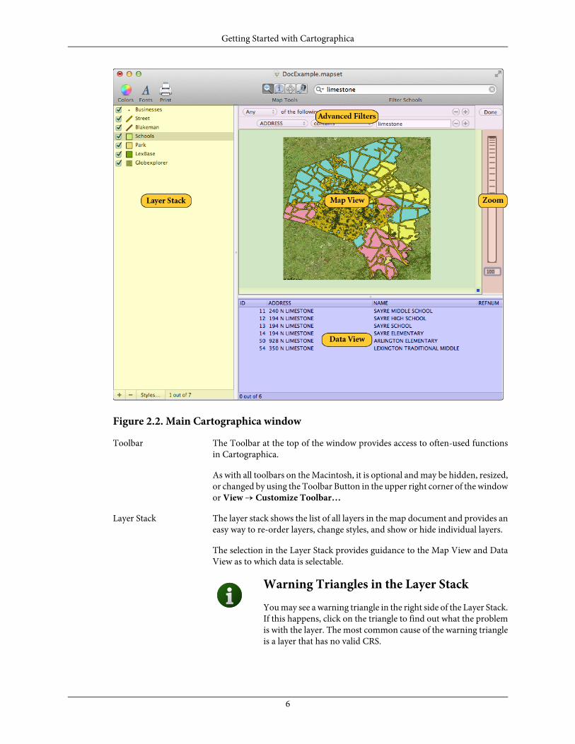
Figure 2.2. Main Cartographica window

Toolbar The Toolbar at the top of the window provides access to often-used functionsin Cartographica.

As with all toolbars on the Macintosh, it is optional and may be hidden, resized,or changed by using the Toolbar Button in the upper right corner of the windowor View → Customize Toolbar…

Layer Stack The layer stack shows the list of all layers in the map document and provides aneasy way to re-order layers, change styles, and show or hide individual layers.

The selection in the Layer Stack provides guidance to the Map View and DataView as to which data is selectable.

Warning Triangles in the Layer StackYou may see a warning triangle in the right side of the Layer Stack.If this happens, click on the triangle to find out what the problemis with the layer. The most common cause of the warning triangleis a layer that has no valid CRS.

6


Map View The powerhouse of Cartographica, the Map View shows your geospatial data incontext with all of the visible layers.

Data View The Data View is used to show and edit data for the layer selected in the LayerStack.

Zoom The Zoom area is used to control and display zoom information about the MapView. The Zoom Dial can be used like a slider to zoom out (slide up) or zoomin (slide down). Below the Zoom Dial is the Zoom Factor Box which shows thepercentage zoom in effect right now. Typing a new value in this box will changethe zoom level directly.

Advanced Filters The Advanced Filters area is not always visible, but once you have started per-forming a filter operation (using the Filter box in the Toolbar), it will pop intoview. Advanced filters provides for boolean operations so that you can searchand filter on more than one variable at a time.

2.3.1. Utility WindowsCartographica uses Utility Windows (sometimes called palettes) that float above other windows in orderto provide access to more information about the current context. The content of these windows is synchron-ized to the current Map Window, so if you have more than one Map open, they will change when youswitch back and forth between the Map Windows. Each of the Utility Windows is accessible via the Windowmenu.

Measurements The Measurements Window provides information about the position directly un-derneath the cursor or the current selection when dragging. See Section 4.5,“Measuring Distance and Area” for details on how to bring up and use the Meas-urement window.

Figure 2.3. Measurements Window

7


#MeasureTool

#MeasureTool

Layer Info The Layer Info Window provides information about the layer currently selected inthe Layer Stack. Changes made in this window affect the data in the selected layer.

Figure 2.4. Layer Info Window

Legend The Legend Window provides a quick reference to all of the layer styles in thecurrent Map.

Figure 2.5. Legend Window

8


Image Viewer The Image Viewer Window provides an enhanced view of any pictures referencedby a feature using the Picture item in the Style window.

Figure 2.6. Image Viewer

Selection Info The Selection Info Window provides a concise view of all selected objects. On theleft is a list of all features currently selected and the layer that they belong to. Onthe right is the information about the selected feature.

Figure 2.7. Selection Info Window

9


Point Data The Point Data Window provides a detailed of all points in geometry of the selectedfeature. On the left is a list of all parts (all geometries have at least one part if theyhave any points). On the right is a list of all points in that part. Point informationmay be edited manually in this window. It is important to remember that all co-ordinates in this window are in the layer's coordinate system, not in the map's co-ordinate system.

Figure 2.8. Point Data Window

2.3.2. The Uber BrowserThe following items are shown inside of the Uber Browser window. The Uber Browser provides a singlelocation to choose from built-in and user-saved symbols, palettes, bookmarks, and other items that areused across all maps. Since Cartographica supports drag-and-drop to do many things, it serves as thestarting point for dragging into other windows. Each tab in the Uber Browser will be described separatelyin this document, as the tabs themselves are where the content lies, however each is accessed through theUber Browser, which can be shown by using Window → Show Uber Browser.

Each tab is described below:

Symbols The Symbols tab provides access to all built-in and user-defined symbols in Cartographica,for use when changing styles for point layers. For more information, see Figure 2.9,“Symbols Tab”

Figure 2.9. Symbols Tab

10


#SymbolBrowser

#SymbolBrowser

Lines The Lines tab provides access to all built-in line styles in Cartographica, for use whenchanging styles for line layers and outlines in polygon layers. For more information, seeFigure 2.10, “Lines Tab”

Figure 2.10. Lines Tab

Patterns The Patterns tab provides access to all built-in and user-defined pattern swatches in Carto-graphica, for use when changing styles for polygon layers. For more information, see Fig-ure 2.11, “Patterns Tab”

Figure 2.11. Patterns Tab

Bookmarks The Bookmarks tab provides access to all built-in and user-defined geographical bookmarksin Cartographica, for use when navigating and exploring in the map window. For moreinformation, see Figure 2.12, “Bookmarks Tab”

Figure 2.12. Bookmarks Tab

11


#LineBrowser

#PatternBrowser

#PatternBrowser

#BookmarkBrowser

Palettes The Palettes tab provides access to built-in and user-defined color palettes that Cartograph-ica can use for vector and raster data. This window provides for selection of palettes as wellas editing. For more information, see Chapter 14, Color Palettes

Figure 2.13. Palettes Tab

2.4. Drag and Drop throughout CartographicaDrag and drop is used extensively throughout Cartographica where it is reasonable. Usually it provides ashortcut to some functionality elsewhere in the program's menus and windows. A few of these drag anddrop shortcuts are elaborated here, but if it makes logical sense to drag and drop something it will mostlikely work.

• Drop vector or raster files on the map window to import them.

• Drop picture files that have lat & long on them into the window and they'll be plotted in a new layer onthe map.

• Drag layers to reorder them in the layer stack.

• Drop one layer on another to copy the styles.

• Drop a color swatch from the color picker onto the map background and change the background.

• Drag a layer from one map window to another in order to create a new copy of that layer in the mapyou drop it on.

• Drop a map icon (grabbed from the title bar) into a Map Layout document to add a map copy there.

• Drop color maps onto analysis layers to change the color map.

2.5. Undo everywhereSince one of Cartographica's key goals is to help you understand your data better, we believe it is importantto be able to quickly experiment with new ways of looking at your data. To help with this, Cartographicais replete with undo and redo capabilities, making it possible to experiment with new ideas to your heart'scontent without having to fear that you'll do something you can't undo.

12


#ColorPaletteOverview

Chapter 3. Importing Data intoCartographica3.1. Overview

Cartographica is commonly used to provide visual interpretations and facilitate analysis of geospatial data.Most data that is analyzed in Cartographica is not created or produced internally. Instead, users typicallyadd data into the maps that have been previously obtained from entities like government agencies or privatebusinesses.

Cartographica imports data from many sources. Using algorithms created by the ClueTrust team and bythe folks who create, maintain, and contribute to Geospatial Data Abstraction Library (GDAL), Cartographicais able to bring in data from an enormous number of sources, including (but not limited to):

• ESRI® Shape Files• MapInfo® MAP Files• USGS DEM and DRG files• Ordnance Survey and GML files• ESRI Personal Geodatabase• GPX files• KML files• ESRI File Geodatabase

The types of files you will use as source data will vary depending upon what you have available and whatspecific needs you have. The general kinds of data that Cartographica can import are:

13

Vector Files Files that contain referenced data in numeric form that can be scaledup to the resolution of the data. Vector data includes data such aspoints, lines, and polygons.

Raster Files Files that contain picture information (such as an orthophoto) ordata sampled at a specific resolution as point sources. Raster Dataincludes data such as pictures or satellite images.

Text Files (or Table Data) Text files can be used to bring in simple geospatial data (such aspoints) or to merge in adjunct information, and usually contain listsof values (or fields). Table data include comma separated values(csv) and tab separated values (tsv). Text/Table import supports avariety of character sets, including UTF-8, WindowsLatin1, andothers. If you are using a non UTF-8 character set, it's best to setthat when opening the file.

GPS Data GPS Devices provide location information sampled at a particularpoint in time. For most purposes, these are waypoints (point sourcesmarked by the GPS User) and tracks (timestamped record of thedevice's travels).

Database Information Databases can contain many of the types of data already describedabove. Although they usually most similarly resemble Text Files(fields of data and possibly simple geospatial data), some databaseformats contain complex geometry.

Figure 3.1. Common File Types

For many applications, a single Cartographica Map Set will contain multiple layers loaded from more thanone type of file or other data source. For example, vector data is often used with an underlying raster imagein order to show it in the context of an aerial photo.

With Version 1.2 of Cartographica, we have introduced the ability to use dynamic maps as well as thestatic maps that we have described so far. These can take on a number of different forms, including vectordata and raster imagery and can come from a variety of sources.

14

Importing Data into Cartographica

Bing™ Maps Bing Maps provides images for use as background maps in Cartographica(and other programs as well as many web sites). The images available includesatellite imagery, roads, and a hybrid combination of the two.

OpenStreetMap OpenStreetMap is a service and an informal protocol. Although the originalOpenStreetMap is a service run from the UK which provides street-levelmap data which has been put together on a volunteer basis around the world,the protocol used by OpenStreetMap has now become an ad hoc standardand is also used by other systems.

Web Map Servers Web Map Servers are servers that use the WMS protocol, defined by theOpen Geospatial Consortium (OGC). This protocol is widely used in privateand public systems and a growing amount of data is available using it. WMSdata is by nature raster data, meaning that it carries no attributes with it. Itis most commonly used as background imagery or to offload complexoverlay tasks to a server so that clients do not need to merge multiple layers.

Web Feature Servers Web Feature Servers are servers that use the WFS protocol, also defined bythe OGC. This protocol is widely used in private and public systems and agrowing amount of data is available using it. Unlike WMS, WFS serves datawhich is, by nature, Features and therefore vector. Data from these types ofservices may be used in analysis and more flexibly understood.

Figure 3.2. Server-Based Formats

3.2. Importing Vector FilesVector files contain geospatial information and often have accompanying reference data that describes thedata in the files.

Procedure 3.1. Importing Vector Files

1. Choose File → Import Vector Data….

The standard file chooser will come up

2. Select the vector file to import and click OK

If you have more than one file to import, you can either select multiple items during this import.

The projection of the map will be set by the first layer added, and projections of each file will be recordedas loaded to make sure each layer is reprojected correctly.

Vector imports are quite straightforward and usually do not require any additional de-cision making, but in the event that your data is in a non-standard character format,you can override the automatic character format detection and select it explicitly. Dataloaded from these files is inserted into the Cartographica system as points, lines, orpolygons (as appropriate) and any per-feature data is added as necessary.

3. Once you have imported the data, choose Layer → Set Layer Projection… to confirm that the coordin-ate system of the data is accurately selected

15


3.2.1. Characters and EncodingsFor shapefiles, Cartographica attempts to figure out what kind of encodings are used in the files by firstchecking for a ".cpg" file (which will be written by ESRI's products when attempting to write out files thatdon't conform to specifications in the DBF format), then looking at the LDID inside of the ".dbf" file itself.

If that fails, the presumption is that the data is in ISO Latin 1, which is the default for older files. We haveconfirmed success working with UTF-8 and many other character sets, but since not all characters arerepresented in the schemes other than UTF-8, there is the potential for losing some data when exportingto other character formats.

In the case of GML and KML, the imported data is presumed to be Unicode UTF-8 (unless specified oth-erwise in the file itself, since there exist ways to do that in these XML-based formats). Other file types mayuse specific characters set in the import window.

3.3. Importing Raster DataRaster files contain data whose form is that of samples in some form of matrix. The most common exampleof this kind of file is an orthophoto image file (such as a JPEG). In these files, the data provided are colorinformation and the matrix is the frame of the picture. Cartographica supports the efficient use of largeRaster files (tested up to 5GB).

Raster files can take on many forms. Some of the more common forms you may want to import include:

• USGS DRG files consisting of georeferenced photo data

• DEM (Digital Elevation Model) Files contain elevation data in a point matrix

• Orthophotos - aerial photos that are geometrically corrected to make the scale uniform

Procedure 3.2. Importing Raster Files

1. Choose File → Import Raster Data.

2. Select the file to import and click Open.

If you have more than one file to import, you may select multiple items during this import.

Some raster data is not georeferenced and may not be positioned correctly on the map. See Section 9.2,“Georeferencing Raster Layers” to solve this problem.

3. Once you have imported the data, choose Layer → Set Layer Projection to confirm that the coordinatesystem of the data is accurately represented (including Datum and Projection).

Once the data is imported, you can use the dedicated layer style window for raster layers to display andchange the color palette applied to the raster data. This is particularly useful for files such as DEM, in whichsamples are made up of floating-point or integer information instead of colors. In addition, by using theTools → Merge Selected Raster Layers you can place more than one dataset in the same layer, forcingthem all to use the same palette over the same range. In automatic mode, the range is the range of alldatasets in the layer. In manual mode, the range is determined by the user.

16


#GeoreferencingRasterData

#GeoreferencingRasterData

3.4. Importing Text Files and Table DataCartographica can import text files that contain tables as geospatial and data sources. Cartographica canuse text files (either CSV, TSV or DBF) to provide three different types of data:

Coordinate data Coordinate data contains either X,Y coordinates or latitude and longitude.

Address data Address data contains postal addresses.

Tabular data Tabular data contains no geospatial information.

Because there is a great variety of sources and types of data which originate in non-geospatial files, Carto-graphica has a few mechanisms that are used consistently in many of our importing systems.

3.4.1. The Import MapCartographica uses the Import Map when importing tabular data (Section 3.4.2, “Importing data fromText and DBF files”) and importing from databases (Section 3.5, “Acquiring Database Data”). It serves twopurposes: first to determine how to associate new data with an existing or new layer, and second, to determinehow to relate the imported data geospatially to the rest of the data in the map.

Figure 3.3. Import Map

The left side of the Import Map window is used to define the relationship between fields within the file ordatabase that is being imported and the layer that they are being imported into. The meaning of eachcolumn is detailed here.

Field Name The name of the field being imported. Based either on the initial line of the file or thedatabase source that the data is coming from.

17


#ImportTableData

#ImportTableData

#AcquiringDatabaseData

Type The kind of data being imported (String, Number, Date, etc). This is determined eitherdirectly from the import source or by heuristic. If necessary, the type information maybe overridden by choosing a different type in the Type menu.

Map To Determines which column this field will map to in the resultant layer. When set to NewColumn, a new column with this name will be added to the table. Special values for geo-coding and Coordinate import are also available. Existing fields are listed if the targetlayer is not new. - Do Not Import - tells Cartographica not to import this field at all.

Key The Key field is only used for the Join style of importing, and we be detailed in sectionREFERENCE. When the Key box is checked, the corresponding relationship betweenthe imported field and the Map To field is used to determine which feature to associatea row from the data file with.

3.4.2. Importing data from Text and DBF filesProcedure 3.3. Importing files containing coordinate data

1. Choose File → Import Table Data….

The import table file chooser appears.

Figure 3.4. Import Table File Chooser

This chooser is a standard file chooser with a few additional options to control how the text is inter-preted. The character set may be chosen, overriding the default character set in the file. For text files,you may also tell Cartographica to consider the first line of the file to contain field names (the default),and designate the column separator and number format.

2. Select the location of the text or table file you want to import and click Open.

The Import Map window appears and describes the format of the file and requests that you determinehow it should interpret the data as it is read.

3. Using Target Layer select an existing layer to append the data to, or choose New Layer.

4. Choose Coordinates from the right hand set of tabs in the window. This will enable coordinate importmode.

18


Because you are in coordinate import mode, the choices in your Map To column include X (or lon-gitude) Y (or latitude), Z (or altitude) and M (or time) along with the standard options of - Do NotImport - , New Column, and any columns that exist in your selected target layer.

5. Using the Import Map (as described in Section 3.4.1, “The Import Map”, map the incoming data fieldsto your selected layer, making sure that you map at least one column to the X and Y coordinates.Without both of these, Cartographica cannot place the data on the map.

6. Click Import to import your data into the map.

Cartographica will read the data from the file, interpret the columns to the best of its abilities andstore them into the requested layer.

7. Once you have imported the data, choose Layer → Set Layer Projection to confirm that the coordinatesystem of the data is accurately represented.

Procedure 3.4. Importing files containing address data

Before importing address data, the geocoder must be appropriately configured. This is an easy process,outlined in Section 8.7, “Geocoding Addresses”.

1. Choose File → Import Table Data….

The import table file chooser appears.

2. Select the location of the text or table file you want to import and click Open.

The Import Map window appears and describes the format of the file and requests that you determinehow it should interpret the data as it is read.


4. Choose Geocode from the right hand set of tabs in the window. This will enable address geocodingmode.

Because you are in address geocoding mode, the choices in your Map To column include Address 1through Address 4, City ,State ZIP, ZIP+4, and Country along with the standard options of - DoNot Import - , New Column, and any columns that exist in your selected target layer.

5. Using the Import Map (as described in Section 3.4.1, “The Import Map”, map the incoming data fieldsto your selected layer, making sure that you map at least one column to Address 1. If it is the onlycolumn specified, then it will be presumed to have a full address in it.

6. If necessary, fill in one or more of the City, State, or Country boxes in the right pane. These act asdefaults for the geocoder in the event that there are no columns that match. Often city data is deliveredwith only the street portion of the address, and these fields can be used to limit the search to thatparticular city.

7. Click Import to import your data into the map.

Cartographica will read the data from the file, interpret the columns to the best of its abilities usingthe geocoding specifications and store them into the requested layer.


19


#UsingImportMap

#GeocodingSetup

#UsingImportMap

3.5. Acquiring Database DataAcquiring database information works similarly to Section 3.4, “Importing Text Files and Table Data”,except that instead of reading the data from a data file, it is read from a database. By using Open DatabaseConnectivity (ODBC) Cartographica is compatible with a wide variety of file formats and database systems(including, but not limited to: Filemaker Pro, Oracle, MySQL, PostgreSQL, and many others).

As with importing tables, Cartographica uses the Import Map (Section 3.4.1, “The Import Map”) in orderto map incoming data to coordinates or addresses.

Due to the nature of the ODBC drivers on the Macintosh, there are some compatibility issueswith older drivers under 10.6 and certain combinations of data and drivers. If you plan toimport data with ODBC, please visit the ClueTrust Knowledgebase and read the article onODBC.

The trickiest part about reading data from a database using ODBC is setting up the ODBC connection onthe system. Although that task is beyond the scope of this manual, there are good documents available fordoing this from the vendors of the connection software. In particular, if you are using FileMake Pro, theyhave a good site, and Actual Technologies provides excellent support for their crop of 64-bit drivers.

As with tables, database data can be interpreted in a variety of ways when it is imported to the system.Coordinate imports, geocoding, and joins are all available for data from databases.

Procedure 3.5. Acquiring coordinate data from a database

1. Choose File → Acquire Database Data…

The Data Source window appears.

Figure 3.5. Data Source Window

2. Select a Data Source and enter a User Name and Password if required.

3. Click Connect and Cartographica will retrieve and present a list of tables.

4. Choose a table from the Table menu to import and click Select.


20


#ImportingTextAndTables

#UsingImportMap

6. Choose Coordinates from the right hand set of tabs in the window. This will enable coordinate importmode.

Because you are in coordinate import mode, the choices in your Map To column include X (or lon-gitude) Y (or latitude), Z (or altitude) and M (or time) along with the standard options of - Do NotImport - , New Column, and any columns that exist in your selected target layer.

7. Refer to Section 3.4.1, “The Import Map” for details on how to map fields with the Import Map window.


Procedure 3.6. Acquiring data from a database

1. Choose File → Acquire Database Data…

The Data Source window appears.

2. Select a Data Source and enter a User Name and Password if required.

3. Click Connect and Cartographica will retrieve and present a list of tables.

4. Choose a table from the Table menu to import and click Select.


6. Choose Geocode from the right hand set of tabs in the window. This will enable address geocodingmode.

Because you are in address geocoding mode, the choices in your Map To column include Address 1through Address 4, City ,State ZIP, ZIP+4, and Country along with the standard options of - DoNot Import - , New Column, and any columns that exist in your selected target layer.

7. At this point, you will be presented with an Import Map window. Please refer to Section 3.4.1, “TheImport Map” for details on how to use the Import Map window.

8. Refer to Section 3.4.1, “The Import Map” for details on how to map fields with the Import Map window.


3.6. Joining Non-Geospatial DataAt times it may be necessary to add data to an existing layer by cross-referencing that data with anothertable. Cartographica does this by matching columns in an existing layer with data from a file and addingthe new data to features which match. This operation is called a join in database parlance and by some GISpackages.

To join data, use the Map To column to specify the destination column for the imported data (or NewColumn if you want to add a new column for the imported data). Matching criteria is specified by checkingthe Key box next to a column. Checking more than one Key box will only add the data when all Key fieldsmatch.

As an example, here is some existing Polygonal data (Example Data A) for three Counties that exist in twodifferent States:

21


#UsingImportMap

#UsingImportMap

#UsingImportMap

#UsingImportMap

Table 3.1. Example Data A - Original Data

Area (Sq KM) State Name County Name1,020KentuckyFloyd1,347VirginiaLoudon989VirginiaFloyd

(Note that Floyd counties exist in both states)

Here is the data you want to join with the above data (Example Data B):

Table 3.2. Example Data B

2000 Census Population 1990 Census Population State NameCounty Name 30,03338,033KentuckyBarren8,2448,243IowaAdair40,44142,441KentuckyFloyd1,099,0001,077,000VirginiaFairfax269,599169,599VirginiaLoudon

Here is the result of performing the Join of Example Data B to Example Data A using County Name andState Name columns as keys:

Table 3.3. Result of original then joined by County Name and State Name as key

2000 Census Popu-lation


Area State Name County Name

40,44142,4411,020KentuckyFloyd269,599169,5991,347VirginiaLoudon

989VirginiaFloyd

In the final table, the extraneous data supplied in Example Data B (Adair, Iowa and Barren, Kentucky)which did not match entries in the existing table is discarded. Further, the lack of data about Floyd, Virginiaresulted in empty columns.

Note that if only the County Name was used as a key and all other columns were matched, then both Floydcounties (the one in Virginia and the one in Kentucky would have values set in all columns, including re-placing the State Name column. However, the explicit use of a multiple key means that Cartographica willonly consider a match when all elements match.

Table 3.4. Result of original joined with just County Name key



Area State Name County Name

40,44142,4411,020KentuckyFloyd269,599169,5991,347VirginiaLoudon40,44142,441989KentuckyFloyd

22


In the case that a feature in the layer matches multiple rows in the joined table, each row from the tablewill replace columns in succession, resulting in the final feature data matching the last matching row inthe table.

3.7. Acquiring GPS DataCartographica supports loading data directly into a mapset from a wide variety of GPS receivers. Importeddata is represented as follows:

Table 3.5. Imported Data

Loaded as lines with each line containing a full trackand missing data being represented by discontinuous

Tracks

lines. Altitude is used as the Z coordinate. Time isused as the M coordinate.Loaded as individual points, with each point contain-ing as much data as is available, Z coordinates areset to altitude if available.

Waypoints

Loaded as continuous lines with each waypoint rep-resented by a single point in the line. Altitude isloaded in the Z coordinate if available. M is ignored.

Routes

Because of ClueTrust's long-standing efforts in Macintosh GPS connectivity (the free LoadMyTracks softwarehas been given away by ClueTrust since 2006), Cartographica supports a large number of GPS devices forimport. Please visit our support site for a detailed listing, but the classes of device and their manufacturersare listed in Table 3.6, “GPS Import Options” along with any special considerations for each type.

Table 3.6. GPS Import Options

Import OptionsSpecial ConsiderationsGPS Type Tracks, Waypoints, RoutesMake sure that your Garmin USB

GPS is plugged in and turned onbefore clicking Acquire.

Garmin USB

Tracks, Waypoints, RoutesSelect the serial port that yourGarmin GPS is connected to andclick Acquire.

Garmin Serial

Tracks, Waypoints, RoutesMake sure that your Garmin Stor-age GPS is plugged in and turnedon before clicking Acquire.

Garmin Storage

TracksSelect the serial port that yourGlobalSat GPS is connected to andclick Acquire.

GlobalSat DG-100

Tracks, WaypointsSelect the serial port that yourGlobalSat GPS is connected to, ac-

GlobalSat GH-615

tivate Data Link to PC mode onthe GPS and click Acquire.

Tracks, Waypoints, RoutesMake sure that your Lowrance GPSdata card is plugged in and moun-

Lowrance

ted on the Desktop before clickingAcquire.

23


#GPSList

Import OptionsSpecial ConsiderationsGPS Type Tracks, Waypoints, RoutesMake sure that your Magellan GPS

is plugged in and turned on andthat data transfer mode is selected.

Magellan GPS

Tracks, Waypoints, RoutesSelect the serial port that yourMagellan GPS is connected to be-fore clicking Acquire.

Magellan Serial

TracksMake sure that your SONY GPS isplugged in and turned on and thatdata transfer mode is selected.

NMEA

TracksMake sure that your Timex DataRecorder is plugged in and turnedon before clicking Acquire.

Timex

WaypointsMake sure that your TomTom GPSis plugged in and turned on andthat data transfer mode is selected.

TomTom

Procedure 3.7. Acquire data directly from a GPS

1. Choose File → Acquire GPS Data.

The Import GPS Data window appears.

Figure 3.6. Import GPS Data Window

2. Select the GPS type from the menu at the top of the window.

3. Choose one or more of Tracks, Waypoints, or Routes to include each of those in your import

4. If you would like an external record of your GPS download, check Save GPX File and a GPX file willbe created while the data is acquired

5. Click Acquire. The data is imported into Cartographica in a new layer.

24


It is not uncommon for tracks to come from GPS devices as single features with multipleparts. Using Cartographica's Split Feature, you can break these down into their constitu-ent pieces. Similarly, if you have too many individual tracks, you can use the MergeFeatures and Merge Selected Layers… features to bring those together.

3.8. Acquiring Images from Web Map Servers (WMS)There is an enormous amount of freely available or paid imagery available on the internet. Even after thepopularity of the internet grew, exchange of imagery data online was difficult due to the wide variety offormats and protocols to access the data. This all changed with the creation of the Web Map Service (WMS)protocol as part of the work of the Open Geospatial Consortium (OGC). WMS provides a standardmechanism for browsing and specifying imagery data available from servers online and declares certainstandards for the transport and representation of that data. Cartographica makes use of WMS to provideaccess to this ready resource of data.

Procedure 3.8. Acquire data from a WMS Server

1. Choose File → Acquire WMS Data.

The Acquire WMS Data Window appears.

Figure 3.7. Acquire WMS Data Window

The server list (on the left) shows a several WMS servers from which you can retrieve data. Once youhave selected a server in the list, the description box below the server list changes to give a description

25


of the selected server as broadcast from the server. The Source list on the right will display the optionsavailable for the selected WMS Server.

2. Select the server in the left column

Cartographica will retrieve the current layer information from the server and present it on the rightLayer column

3. Select one or more layers on the right

The Layer list on the right shows layers that can be added to your maps from the Server. Data markedwith a red (-) cannot be added (usually because it is a category) and data marked with a green (+) canbe added. When one of these sources is selected, a description appears in the box below the Sourcelist.

In some cases, multiple layers can be added in the same request. If there is a limitation on the numberof simultaneous layers that may be chosen, it will be displayed in the lower left.

4. Select the Coverage Area to determine how much information is downloaded from the server. Thedefault Visible map bounds is generally suitable as it adds a margin around the current map's extent.Selected layers will limit the bounds of the imagery to the extent of the selected layers, and Mapbounds will limit the bounds of the imagery to the extent of the current map, without any margin.

5. If want to download a copy to disk (as opposed to always fetching data from the server),checkDownload as Static Imagery

Checking this box will download a single map to your hard drive. The quality of the imagery whenyou zoom will be decreased, but you will be able to work on the map even when you aren't connectedto the server, and your imagery will never change.

6. Click Retrieve to add the data to your map.

Procedure 3.9. Add New WMS Server

When you have the WMS Server sheet visible, you can add more servers to the source list on the left

1. Click the Add (+) button at the bottom of the left column to start adding a new server

The Add new WMS Server window appears.

Figure 3.8. Add Map Server sheet

26


2. Enter the name of the server and the URL and click Add. The Server will appear in the source list onthe left.

Procedure 3.10. Removing a WMS Server

When you have the WMS Server sheet visible, you can remove servers from the source list on the left

1. Select the name of the server from the source list on the left

2. Click Remove (-) beneath the source list

Procedure 3.11. Editing a WMS Server

When you have the WMS Server sheet visible, you can edit servers from the source list on the left

1. Select the name of the server from the source list on the left

2. Click Edit… beneath the source list

3. Change the name of the server and/or the URL and click OK

27


Chapter 4. Exploring DataCartographica is first and foremost a tool for exploration of data. This chapter describes many of the toolsavailable for visualizing the data that you have. In concert with the analysis and presentation features, thesetools provide a robust starting point for understanding the information within your data.

4.1. Zooming In and Out of MapsThere are several ways to zoom in and out of a map:

• Use the scroll wheel on the mouse while holding down the Option key on the keyboard

• Use the Zoom Dial on the right side of the Map Windows

• Use the Zoom To menu items in View to jump to particular zoom levels

• Use the zoom tool to zoom to points or areas using the mouse pointer

• Use the Previous and Next Extent items in View move to the previous or next zoom locations

Figure 4.1. Zoom Dial

28

Click and hold the zoom dial and move it up to zoom in and down to zoom out.

You can also zoom by clicking your mouse when you are using the Zoom tool. The Zoom tool also has atoolbar icon looks like this:

When the Zoom tool is selected, the cursor becomes a small little magnifying glass. Click anywhere in themap to zoom in and center the map on that point. To zoom back out, click while holding the Option keyon your keyboard.

You can also zoom by selecting an area with the mouse (like drawing a box around it) when you have theZoom Tool toolbar icon selected. You will zoom in to the borders of the box you just drew.

To go to the last Zoom use the Previous Extent/Next Extent menu options available in the View menu.Essentially, these options are undo/redo for zooming.

4.2. Selecting Data and Using the Identify ToolThe Identify tool allows you to draw around an area of features on the map or click one feature directlyand make the data about that feature appear in the data window. The Identify tool toolbar icon looks likethis:

Use the Identify tool to identify any feature in the currently selected layer. When you select the feature byeither clicking on it, or surrounding it with a rectangle that you can draw (also good for selecting multiplefeatures) the chosen items are highlighted in the data window.

For additional information display, Choose Window → Selection Info to display the Selection Info window,which displays a scrolling list of information about each selected item. This is particularly useful if youhave a lot of items selected which aren't next to each other in the data view, or if you have closed the dataview to maximize map area.

FIGURE OF SELECTION INFO WINDOW

4.3. Using the Pan Tool to Move a MapYou can use the Pan tool to grab and move the map to change the view. The Pan tool toolbar icon lookslike this:

Once you have selected the Pan tool toolbar icon, the cursor becomes a small hand with which you canmove the map within the map window. Click the mouse at any point and then drag to move the map.

4.4. Data TooltipsData Tooltips show you summary information about selected features. By holding down the Option keywhile moving over any item in the selected layer, a small window will appear with information about theitem you have moved over. The information that appears is defined in the Layer Info window.

29

Exploring Data

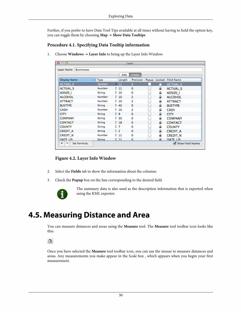
Further, if you prefer to have Data Tool Tips available at all times without having to hold the option key,you can toggle them by choosing Map → Show Data Tooltips

Procedure 4.1. Specifying Data Tooltip information

1. Choose Windows → Layer Info to bring up the Layer Info Window.

Figure 4.2. Layer Info Window

2. Select the Fields tab to show the information about the columns

3. Check the Popup box on the line corresponding to the desired field.

The summary data is also used as the description information that is exported whenusing the KML exporter.

4.5. Measuring Distance and AreaYou can measure distances and areas using the Measure tool. The Measure tool toolbar icon looks likethis:

Once you have selected the Measure tool toolbar icon, you can use the mouse to measure distances andareas. Any measurements you make appear in the Scale box , which appears when you begin your firstmeasurement.

30

Exploring Data

Figure 4.3. Scale Box for Measuring

In the Scale box:

• X and Y show the location (in map coordinates) of the mouse click (or just of the location of the cursorif you are not holding down the button).

• X2 and Y2 show the location (in map coordinates) of the cursor if you are holding down the mousebutton.

• ∆X and ∆Y show the coordinate differences between X and X2, and Y and Y2 respectively (also in co-ordinate units).

• Distance is the distance of a straight line from X,Y to X2,Y2 in linear coordinates.

• Area is the area of a rectangle bounded by "X","Y" and "X2","Y2" in linear coordinates. Essentially theline you create is making the diagonal for a rectangle that is bound by those points.

"∆X" and "∆Y" are in linear or angular coordinates depending upon the coordinate systemof the map. However, distance and area are always in linear coordinates, using the great-circle method when the coordinate system of the map is natively angular.

• Bearing is the bearing (relative to the X axis of the data) from X,Y to X2,Y2.

To change the units for the measurements, select one of the gear drop down menus in the measurementwindow and choose the units. Units can be controlled and the scale itself may be restricted to a fixed size(in units). When using fixed unit size, the units will be adjusted to the next larger unit if the value couldnot be displayed in the available space.

31

Exploring Data

Figure 4.4. Measurement Window Drop Down menu

To use the tool to measure distance:

To measure a line or distance between two points, select the Measure tool toolbar icon. Click on the firstpoint from where you want to measure, hold the mouse button and drag the cursor to the second point.The distance between those points will be displayed in the Measurement window.

To measure area, select the Measure icon, place the cursor over one boundary corner of the area you wantto know and then click and hold the mouse button down until you drag the cursor to the other boundarycorner of the rectangle you want to measure. The area of the rectangle appears in the Measurement window.

4.6. Using the Data ViewMost GIS data has geospatial information in the form of features (points, lines, and polygons) and non-geospatial data, which may consist of just about anything you can imagine: place names, number of crimesin an area, type of pavement on road. This data is sometimes displayed on the map as labels, representedby colors, or visualized in other ways.

The data view is located at the bottom of the main Cartographica window. This is a standard Mac OS Xtable, and works the same as other tables on the platform.

32

Exploring Data

Figure 4.5. Data View

The layer that is shown in the data view is the layer that is currently selected in the layer stack. If you arelooking at the screen and wondering why the data you're looking for is not what you expect, check thelayer stack and make sure the layer you are interested in is selected. If you have more than one layer selectedin the layer stack, no data will be shown in the data view.

Further, the selection in the data view is synchronized with the selection in the map view, which meansthat if you select a feature in the map view, the data view will scroll such that the information about thatfeature is visible. Similarly, if you click on a row (or rows) in the data view, the corresponding map viewfeatures will be selected.

Procedure 4.2. Sorting the Data View

1. Click on the heading for the column on which you would sort the view

The table will sort to your specifications and an arrow will be displayed at the right side of the headerto indicate the sort order.

2. To sort in the opposite order on the same column, just click again in the column heading.

Procedure 4.3. Re-ordering columns in the Data View

• Click on the column heading and drag it to the new location

The column will move from its old location to the new location

Procedure 4.4. Editing data in the Data View

Editing most of this data is very straightforward as it is done directly in the data table below the main Mapin the Map Window. Once you have a layer selected, click on the individual cell of data and start typing.

1. Select a single layer in the layer stack

Cartographica will display the data for this layer in the data view

2. Select a feature:

• Click on a feature in the map

• Click on a row in the table

The feature will be selected in both the map and the Data View.

33

Exploring Data

3. Click in the column to change

The blue focus box will show up around the table cell indicating that you may now enter your data

Columns which have been locked or which contain Column Formulas cannot be editedand will not enable when clicked.

4. Press the enter key to finish editing

Procedure 4.5. Locating the selected data on the map

There are times, especially when working with the Data View that you can't easily locate the data you haveselected on the map. Cartographica has a couple of different ways to view these.

1. Select the item that you want to locate on the map using the Data View

2. Tap and hold the space bar•

The selected feature(s) will appear zoomed out to the full size of the Map View. When the spacebar is released, the feature will recede slowly into its position on the map. This is most usefulwhen you just want to locate, but not move the focus of the map

•

• Choose View → Zoom to Selected Feature

The Map View will be zoomed to an area encompassing the selected feature(s). This is mostuseful when you are interested in seeing the detail of a feature.

3. Click on the heading for the column on which you would sort the view

The table will sort to your specifications and an arrow will be displayed at the right side of the headerto indicate the sort order.

4. To sort in the opposite order on the same column, just click again in the column heading.

Procedure 4.6. Re-ordering columns in the Data View

• Click on the column heading and drag it to the new location

The column will move from its old location to the new location

4.7. Adding, Removing, and Renaming ColumnsColumns may be added to and removed from any layer. There are some restrictions on exactly how this isdone.

Table 4.1. Column Change Restrictions

RestrictionsLayer TypeColumns added to By Reference layers will requireeither internal saving or updating the original file to

All By Reference Layers

34

Exploring Data

RestrictionsLayer Typekeep their data. This only happens when you savethe Map Set, so if you are doing this temporarily thereis no harm. The only exception to this are FormulaColumns, which are only stored in the Map Set andcan continue to use the By Reference data.Columns added to WFS Layers will not create newcolumns on the server. Any data that is added to

WFS Layers

these layers will be lost when the Map Set is savedand re-opened. As with By Reference layers, FormulaColumns will have their data recomputed on loadand thus will not be lost when saving a Map Set.There are no features and thus no columns for LiveMaps.

Live Maps

Columns of any data type may be added in Cartographica. By default, the Add Column command fromthe Layer menu will add a String column, which can represent textual or numeric data.

Procedure 4.7. Adding Columns to a Layer

1. Select the layer in the Layer Stack

2. Choose Windows → Show Layer Info to bring up the Layer Info window

3. Click the Fields tab to show the list of columns

4. Click +•

• Choose Layer → Add Column

A new column will be added to the column list and brought into view

5. Optionally change the type of the column by selecting from the corresponding Type cell

6. Optionally change the size of the column by clicking in the corresponding Length cell

Procedure 4.8. Removing Columns from a Layer




4. Select the column to remove

5. Click -•

• Choose Layer → Remove Column

The selected column will be removed from the column list

35

Exploring Data

Procedure 4.9. Renaming Columns in a Layer




4. Select the column to rename

5. Click in the corresponding Name cell and type the new name

The selected column will be renamed

4.8. Using the Selection WindowThe Selection Window shows information about the features you select in the data window. To access theSelection window, go toWindow → Show Selection Info.

Figure 4.6. Selection Window

The Selection Window is best used for looking at specific data when you have multiple items selected inthe map or data view.

The left-hand side controls what information is available in the right-hand side. By double-clicking on theleft hand side, the Data View and the map view window will change to show only those items selected inthe column on the left-hand side.

4.9. Using the Point Data WindowThe Point Data window is used for looking at the detailed geometric data of a feature. To open the PointData window, choose Window → Show Point Data.

36

Exploring Data

All data in the Point Data window is expressed in the original coordinates. Modifying geometric pointswill cause those points to be reprojected onto the current map's coordinate system.

Generally, it is easier to edit if Maps and Layers are (at least temporarily) set to the same value.


Use the left side of the window (Part) to select the part within the feature (many features have only onepart, but others may have many). The right side of the window (Point) shows the list of points in the selectedPart. In the case of a Line, a part describes disjoint line segments. In the case of a Polygon, the parts describeislands or holes in the Polygon.

4.10. Additional Layer InfoFrom the Layer Info Window click the Info Tab. The Info tab appears.

37

Exploring Data

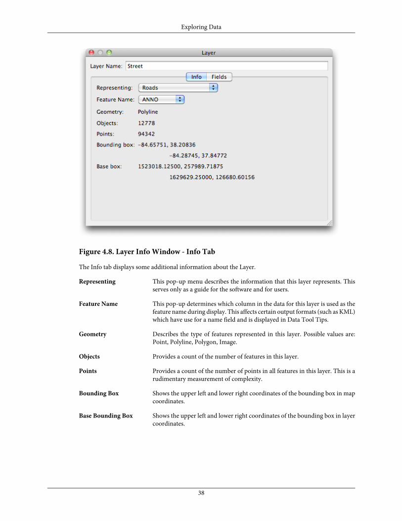
Figure 4.8. Layer Info Window - Info Tab

The Info tab displays some additional information about the Layer.

Representing This pop-up menu describes the information that this layer represents. Thisserves only as a guide for the software and for users.

Feature Name This pop-up determines which column in the data for this layer is used as thefeature name during display. This affects certain output formats (such as KML)which have use for a name field and is displayed in Data Tool Tips.

Geometry Describes the type of features represented in this layer. Possible values are:Point, Polyline, Polygon, Image.

Objects Provides a count of the number of features in this layer.

Points Provides a count of the number of points in all features in this layer. This is arudimentary measurement of complexity.

Bounding Box Shows the upper left and lower right coordinates of the bounding box in mapcoordinates.

Base Bounding Box Shows the upper left and lower right coordinates of the bounding box in layercoordinates.

38

Exploring Data

#ExportingToKML

#DataTooltips

Chapter 5. Working With Layers5.1. Using the Layer Stack

The Layer Stack appears on the left side of the Cartographica Window. This view shows all of the differentlayers of data that appear in the map.

Figure 5.1. The Layer Stack

The Layer Stack defines what appears in the Map View and Data View.

You can drag items to re-order them in the layer stack. Top is "on top" if you were to think of it as a layercake or a set of papers layered on top of each other. Often, if you are using a raster layer, you'll drag thatto the bottom so that all the vector content sits "above" it.

You can also drop a layer on another layer to copy styles from the dropped layer to the dropped-on layer.Although it might seem strange, you can also drop a layer on another layer of a different type. This allowsfor an easy way to copy the color schemes.

Procedure 5.1. Showing and Hiding layers

You can choose which layers are shown on the map by

• Toggling the box next to the layer name in the layer stack•

• Choose Layer → Hide Layer or Layer → Show Layer

When you do hide a layer the features contained in this layer are no longer seen on the Map.

5.2. Using the Layer Info WindowThe Layer Info window shows the data features of the layer that is selected. It is used to add/remove columns,change data types, and modify column names. To access the Layer Info window, choose Window → Showlayer Info. The Layer Info window appears showing the Fields tab.

39

Figure 5.2. Layer Info Window - Fields Tab

5.3. Filtering on Layers Using the Filter BoxYou can use the Filter Box from the main window to filter map data within a layer and to create new datalayers with the results. The Filter Box appears in the top right of the main Cartographica window.

Figure 5.3. Filter Box

Enter the data you want to filter into the search box. As you type, the results are narrowed and are displayed(filtered) in the data window. This filter is extremely fast, even for large datasets and is the preferredmethod for finding an item in the data window. Use the Filter Box with Layer/Create Layer from Selectionfrom the Layer menu to split off data that is interesting for further analysis. The filter operates on the layercurrently selected in layer stack. The filter works by filtering the data in the selected layer as shown in boththe data and map views. You can also use extensions such as commas to further filter results.

And/or and multiple-field data filtering is now possible and easy with this new system. The existing filterbox works as a short-cut, translating queries into the new system, which can then be edited.

As you type into the filter box, you will see a drop-down area at the top of the Map View that contains amuch more flexible filtering system.

40

Working With Layers

Figure 5.4. Advanced Filter Box

You can select which filter or all filters to use by selecting either Any, All or None of the following aretrue.

The first selection drop down menu (shown as info.Capital in the screen above) is a menu to select whichcolumn in the data window you want to search.

Then you can select if you want the filter to be is the less than, is greater than, or is, or contains the filterphrase.

The text box contains the text you enter that you want to filter on.

You can click the + or - button to add or remove additional filters.

Click the Done button to dismiss the additional Filter boxes and restore the maps and data views to allfeaturesin the selected layers.

You can also filter using variables from the same or multiple fields. This is useful for creating new layers.

5.4. Adding and Removing LayersAlthough most layers are added to Cartographica map sets by importing them from existing files or networkservices, it is quite reasonable to create a layer yourself. Most frequently the goal of adding a layer ismanually create some new features (such as drawing an area over an existing map).

Procedure 5.2. Adding New Layers

1. Choose Layer → New Layer•

• Click on the Add(+) button under the Layer Stack

The new layer is added with no data and the a default name

2. Click on the name in the Layer stack to select the text and then replace with your new name

Procedure 5.3. Removing Layers

1. Select the layer you wish to remove in the Layer Stack

2. Click on the Remove(-) button under the Layer Stack•

• Choose Layer → Delete Layer

The selected layer is removed

41

Working With Layers

5.5. Adding a New Layer Based on a Data SelectionIf you want to create a new layer from a selection of data in your map, select the data you want to add to anew layer in the Data window. Now, Layer → Create Layer from Selection.

You can also select a data set using the filter bar to create a filtered list of data to create a new layer from.

This creates a new layer that will appear in the Layer stack from the selected features in the current layer,copying the styles and all data attributes.

5.6. Merging LayersCartographica can merge layers with similar data into a single layer, creating a new layer with the contentsof all the selected layers, and removing the original layers.

This is commonly used to put like data together in a single layer for easy manipulation.

Consolidating layers will remove all of the selected layers from the map and replace them with a singlelayer that has all of the features of the selected layers.

• Layers must contain the same kinds of features (points, lines, or polygons).

• Layers with different dimensionality (2D, 3D, or 4D) will be upgraded to the highest dimensionality ofthe set.

• Optionally, you can choose to consolidate data fields for layers containing columns of the same nameby clicking the Consolidate data fields with the same name checkbox. Columns with different nameswill be appended and the data for the other features will be left blank.

1. In the Layer Stack, select the multiple layers you want to merge, by command-clicking the mouse oneach layer.

2. Layer → Merge Selected Layers.

The Merge Selected Layers dialog appears.

42

Working With Layers

Figure 5.5. Merge Selected Layers

3. If you would like to add a column to each entry in the new layer stating which layer the entry originatedfrom, click the Add original layer name in From Layer field checkbox.

4. Choose which Layer the styles come from using Inherit styles from drop down box.

5. Now click Consolidate.

5.7. Masking Data for Analysis LayersWhen using an analysis layer (for now only created by the Kernel Density Map), often the analysis layerhas a significant amount of data falling "outside" of the area of interest. To help remedy this, Cartographicacan constrain the bounds of the analysis layer to the area of a polygon layer.

Below are examples of an analysis layer, the mask to be applied, and the resultant masked analysis layer.In this case, we use a Kernel Density Map and have a satellite map in the background as illustration.

Figure 5.6. Analysis Layer without Mask

43

Working With Layers

Figure 5.7. Analysis Layer Mask

Figure 5.8. Analysis Layer with Mask

Procedure 5.4. Masking an analysis layer

In order to mask an analysis layer, you need to have a polygon layer that specifies the area you want includedin the analysis. You can either use an existing polygon layer, or create one manually or using tools such asCartographica's Tools → Make Convex Hull

1. Select the analysis layer in the layer stack by clicking on it

2. Select the polygon layer in the layer stack by holding the option key while clicking on it

3. Choose Layer → Set Mask Layer

After a few seconds, the analysis layer will be masked by the polygon layer you selected.

The mask layer will work even if the mask layer is hidden, so you can add a layer to actas the mask, assign it to the analysis layer, and then hide the mask layer without losingthe mask effect, but without having whatever data is in that layer displayed.

Procedure 5.5. Removing an analysis layer mask

1. Select the analysis layer in the layer stack by clicking on it

2. Choose Layer → Clear Mask Layer

5.8. Setting Layer ProjectionIn the event that a layer of data is imported without any projection information, Set Layer Projection canchange the projection without modifying the data.

44

Working With Layers

It is common for data that comes in csv form to be delivered in a State Plane Coordinate System insteadof Latitude/Longitude (which will be automatically selected in most cases). In the case that the projectioninformation is not there, use the following process to set the layer projection.

1. Layer → Set Layer Projection to set the layer's projection information.

The Set Projection Layer dialog appears.

Figure 5.9. Set Projection Layer Window

Setting the projection here will change the projection for this particular layer, but it will not change theshape data. Changes will be saved in the map file and possibly in an associated PRJ file.

2. From the left side of the dialog, choose the map projection that best suits your needs.

The Description box on the right will change depending which projection is selected. You can also clickthe Specifications tab to see additional details about the selected projection.

Below this informational area there is a small preview area that gives a general orientation for the featuresof your map once the selected projection has been confirmed.

Here you should use the filter box to search for a projection.

The feature projection shape is previewed on the right side of the window so you can get an idea of whatthe selected projection will look like.

3. Once you have the selected the projection that best suits your needs and most accurately represents thedata you are attempting to display, click Set.

45

Working With Layers

5.8.1. Reprojecting LayersCartographica allows users to change the geographic projection of data to several predefined datums. Thelimited applications include preparing data for export in another CRS.

For example, if you need a shape file in WGS84, but you have data in State Plane, you can use ReprojectData to change the data from the State Plane to WGS84 and then use the Export Layer command to exportit.

This is seldom the case, so most often, you can use Map → Project Map to set the map pro-jection or Layer → Set Layer Projection to change how the features in a particular Layer areinterpreted.

To permanently change the map projection:

1. Layer → Reproject Layer.

The Reproject Layer dialog appears.

Figure 5.10. Reproject Layer dialog

Changing the projection here will permanently modify the shape data to correspond to the selectedprojection. If you reconvert it back to the original, it is likely that a loss of accuracy will occur. If you'renot certain you want to do this, set the projection.



46

Working With Layers

Below this informational area there is a small preview are that gives a general orientation for the featuresof your map once the selected projection has been confirmed.


5.9. Referenced DataCartographica tries to be intelligent about referencing external data in order to maximize efficiency andconvenience. In many cases, Cartographica can make an external reference to a file instead of making itpart of the Mapset. This data is referred to as being Externally Referenced.

When a layer is Externally Referenced, it has a by reference icon in the layer stack on the right side. Also,when that layer is selected, the Layer menu's Include Layer Data in Mapset item is unchecked.

Often, storing boilerplate data and large imagery in external files is desired to save space and to make up-dating that data easy. Imagine having a set of 10 maps that all need road information, but your road inform-ation changes on a monthly basis. If your road polygons are kept in an external file, you need only updatethe external file, load your mapset and the information is up-to-date.

The main reason to use this is if you need to "Freeze" the data for a particular layer so that you don't acci-dentally change it.

Procedure 5.6. Bringing External data into the Mapset

1. Select the desired layer from the Layer Stack

2. Choose Layer → Include Layer Data in Mapset to bring the data into the Mapset. The next time yousave, a copy of the data will be made inside of this Mapset.

Once a data set it brought into the Mapset, the only way to make it external again is to delete the layer withthe internal copy and re-import the data.

Occasionally, you may need to create a copy of a Cartographica Mapset for distribution to other parties orto archive the complete state of a map and all its constituent parts. In this case, often it is necessary to putall of the data into the Mapset file before sending it because the recipient may not have the original files.Since permanently changing this might not be desired, you can save a copy of your Mapset file that hashad all of its layer data brought internal, or "flattened".

Procedure 5.7. Flattening a Mapset

1. Choose File → Save As to begin the saving process

2. Check Flatten Map When Saving to flatten the file

3. Now choose a file name and click Save

47

Working With Layers

Chapter 6. Working With StylesStyles determine how a map looks when viewed, printed, embedded in a map layout, or exported to anystyle-conscious format (such as Adobe Illustrator or KML).

Cartographica has a sophisticated style system which provides significant control over how data is shownon the screen and in printed output.

Styles are assigned and manipulated for each layer individually.

Procedure 6.1. Opening the Style Editor

To bring up the Style Editor for any layer, use one of the following techniques:

1. Select the desired layer in the Layer Stack

2. Double-click on the layer to open the Style Editor•

• Click on the Styles… button at the bottom of the Layer Stack to open the Style Editor

• Choose Layer → Show Layer Styles

At this point, you should have an appropriate Style Editor Window visible.

48

#ExportingToIllustrator

Figure 6.1. Layer Styles Window (showing a complex polygon layer)

6.1. Styling Vector LayersStyles in Cartographica are a very powerful mechanism for changing the presentation of your map. By usingthe values of data in the features, Cartographica can create thematic maps without requiring manual inter-vention in every step of the process.

When Cartographica prepares to draw a particular feature, it first evaluates the style, as defined in the layer'sStyle Window, to determine if the feature qualifies for a particular style variation, or if it is to be drawnwith the Default Style. For layers where you desire all features in the layer to look the same, use only thedefault style and all features will be drawn the same.

Vector styles share many traits, although each different type of feature (lines, polygons, and points) havesome unique attributes and slight variations in how the standard attributes are applied.

For all style manipulation, work begins in the Style Window.

49

Working With Styles

Figure 6.2. Style Window (displaying a complex point style)

The style window is divided into three primary areas:

• The upper left portion of the window contains the Style List, which is used to discriminate between stylesin a style set. All layer styles can either be comprised of a single style (in this case, referred to as the DefaultStyle) or multiple styles. This will be covered later in Section 6.1.5, “Complex Styles”.

• The right side of the window is the Appearance pane and it determines how each feature in a particularstyle looks. This includes the label, marker, lines, colors, and naming.

• The lower left portion of the window is a Preview of the style you are currently working on. In the caseof multi-style style sets, the selection in the Style List determines which style is shown in the Preview.

Since many of the elements of the Appearance pane are common to every feature type, we will examinewhat each element represents and how it is used, going from the top to the bottom.

• Name is used in the Map Legend and other areas of the software to represent this particular style in astyle set. The contents of this field are used as the name of the style in the legend, when multiple stylesare shown. If you leave the Name field empty, Cartographica will create defaults based on the values thatcomprise the style's range.

• The color wells are used to adjust the color of individual elements. Their use varies based on the type offeatures represented by the layer, and by the element that is being styled. Color wells function as drop

50

Working With Styles

targets and bring up the color picker when they are clicked on, allowing you to choose colors using thestandard mechanisms available to all Macintosh software.

• Size fields are denoted by a slider and a text area and allow you to change size parameters, such as linewidth, pattern size, or symbol size. The slider and the box both provide the same control, and you canuse them interchangably.

• Item Label and Insert Field menus are used to determine what text should be placed next to the point,along the line, or inside the area. You can add text to the label by typing into the box, and references tofields can be added by placing the cursor where you want the field and then using the Insert Field pop-up menu to select the field you want added. A field marker (with the name of the field inside of a coloredcell) will be placed at the cursor location. This is covered in depth in Section 6.1.4, “Labeling Features”

• Always show labels determines if labels are always shown for this particular style, or whether the systemshould determine whether they should be visible or not. Generally, you should leave this unchecked formost styles, but if you have features whose labels you always want displayed, this box provides allowsyou to override that.

• Symbol, Picture, and Picture Path are only available when editing Point features, and so they will becovered in Section 6.1.1, “Point Styles”.

6.1.1. Point StylesPoint styles can be customized in many ways. The Size slider and box control the total size of the pointitem. Due to variations in particular symbol drawing techniques and different visual weights (which affectapparent size), it is often the case that symbols with the same size are similar, but not identical in size orarea. This is to be expected. We have tried to keep the sizes consistent for all symbols created directly insideof Cartographica, but you may need to balance sizes a bit, especially when using custom picture- or font-based symbols or when using symbols of greatly differing weights.

For most Point symbols, the Stroke box and color well determine if the outline of the symbol is visible andthe color of the symbol outline. Not surprisingly, the Fill color well determines the color which fills in thesymbol. For some symbols, there is no "fill" area, and therefore the symbol's fill color does not matter andthe stroke must be present for the symbol to draw. Examples of these in the built-in symbols are the crossand plus.

Although Cartographica may not ship with the variety of symbols of some other programs, the ability toimport high-resolution symbols from a variety of places makes up for many missing symbols. To changea symbol, the Symbol Well is used as the dropping point for one of a variety of sources:

• The Symbols Browser window, which is the built-in repository for scalable symbols (pictured in Figure 6.3,“Symbol Browser Window”), contains a number of common symbols for use on maps which are simple,but highly scalable.

• Images from a variety of sources. Basically any image that you can get onto your Macintosh is usable asa symbol in Cartographica. This can be a graphic from a web page, something designed in illustrator, ora licensed piece of clip-art. When an image symbol is used, Cartographica pays attention to the alphachannel for transparency, meaning that transparent-capable formats such as PNG are more desirablethan JPEGs, as an example.

When using images as symbols, the Stroke and Fill colors can seem to behave oddly. Thisis because, when checked, the Stroke will color anywhere in the image that is not transpar-ent, and the Fill will not be used. For graphics that have transparency, this can have thedesirable effect of being able to color the parts of the image with color. However, forgraphics that contain black and while colors (for example), it has the surprising effect of

51

Working With Styles

coloring the entire symbol (white and black) with the stroke color. To turn off the colormanipulation, just uncheck Stroke.

• The Macintosh Character Viewer. The Character Viewer is a standard part of OS X, which is madevisible on the screen by checking the Show Keyboard & Character Viewer in menu bar option in theKeyboard preferences panel in System Preferences. Once this box is checked, you can bring up thewindow by choosing Show Character Viewer from the menu bar. Any character from the palette canbe made into a Cartographica symbol just by dragging it into the Symbol Well. Among the availablesymbols in many standard fonts are: airplane, a variety of stars, and many more. Plus, cartographicsymbol fonts are also available from a variety of commercial and non-commercial providers.

• Stylized text from any window. Although single-characters are often enough and our labeling systemprovides ample opportunity to provide static and variable text labeling, text from any window can alsobe used as a "symbol" for a point.

Besides symbols, Cartographica can also represent points with a picture stored on disk by using the Picturecheck box and field selector and optionally the Picture Path to specify the location of the referenced pictures.When using a picture to represent the points on the map, the Picture box must be selected and a field mustbe chosen in the pop-up menu. The picture field designates which column contains the file name of thereferenced file, which can be a full or partial path name. A partial path name is resolved first by looking atthe Picture Path and then by using the directory the layer (or map set for an internally-stored layer) issaved in as the default. When using a picture symbol, the Image Viewer will come up whenever a repres-ented point is selected, showing a larger version of the picture (or a playable version of the movie, if thereferenced data is a movie file).

Figure 6.3. Symbol Browser Window

Labels may also be added to point features, see Section 6.1.4, “Labeling Features” for further information.

Procedure 6.2. Setting the Symbol for a Point layer

1. Open the Style Editor for the desired layer

2. Click once in the Symbol well in order to bring up the Symbol Browser Window.

3. Choose a symbol from the Symbol Browser Window and drag it to the Symbolwell

4. Adjust Point Size,Stroke, and Fill as desired

Procedure 6.3. Using a Font Character as a Symbol for a Point Layer


52

Working With Styles

2. Bring up a window containing the font character. Commonly this is done with the Show CharacterViewer item from the menu bar (if you can't find it, you may need to turn it on in the Keyboard SystemPreferences

3. Choose a symbol from the character viewer or other window and drag it to the Symbolwell


Procedure 6.4. Using an Image File as a Symbol for a Point Layer


2. Bring up a Finder window containing the symbol file

The file should be one of the standard image types understood by the MacOS X, suchas: PDF, Adobe Illustrator, GIF, JPEG, PNG, etc.

3. Drag the file to the Symbolwell


The effect of the Stroke and Fill on image symbols can be a bit strange. Generally, youwill want to use the Stroke box and color only if you want to completely fill the symbolwith the stroke color.

Procedure 6.5. Using Pictures as a symbol

Before using pictures as a symbol, you must make sure that you have the picture files in a format that MacOSX understands, such as JPEG, GIF, or PNG. You must also know where those files are in relation to thePicture Path or the layer data.

These instructions assume that you already know where the pictures are and have a column that containsthe partial or full path names to the picture files.


2. Select the name of the column with the paths by using the Picture pop-up

3. If your photos are referred to by partial path names, you may need to select the Picture Path by usingthe pop-up menu

4. If you would like the pictures to show up in the map as the Point symbol, make sure the Picture boxis checked

To change the size of the displayed picture on the map, use the Point Size slider or box.

53

Working With Styles

6.1.2. Line StylesLine styles can be used to change the visual aspects of lines on a map. Some of the components for linestyles should now be familiar to you, based on the point styles, but lines have some additional attributes.

Line styles are based on a line style template, which are dropped into the line style well in order to assignthem to a style. In the example shown below, the Default Style for this line contains a line with thin blackstrokes, and a yellow fill. Not all lines will have both parameters, however they should all have a Strokecolor, so that you can change the overall color of the line style. In some special cases, there are colors inthe style that are not able to be changed through this window. If you are using one of these styles and findthe need to change the color, look for another line style in the Lines tab of the Uber Browser.

The Width determines the width of the line, and in the case of a stroked line, the width of the stroke aswell. The two are proportionate, and therefore the width is a scaling factor that operates equally on eachof the components of the line.

Figure 6.4. Style Window (displaying a complex line style)

Procedure 6.6. Setting the Line Style


2. Click on the line style well next to the color wells

54

Working With Styles

The Uber Browser will appear with the Lines tab selected.

3. Choose a line style from and drag it to the line style well

The line style should change in the well, the preview, and on the map to reflect your choice.

4. Adjust Size,Stroke, and Fill as desired

6.1.3. Polygon StylesPolygon styles can be used to change the coloring, pattern, outline style, and labeling of polygon featureson the map. You can leverage much of your knowledge from the line and point styles to use the polygonstyle window. In fact, the window is even set up to reflect this, with the Outline box in the top position(where the Line box appears for lines), and the Pattern box in the lower position (where the symbol boxappears for poings).

When a polygon is drawn, Cartographica uses the Outline information to draw the outline of the polygon,and the Pattern information to fill in the inside of the polygon.

The patterns in Cartographica work similarly to the Symbols in point layers. There are certain pre-definedpatterns that come with Cartographica, and they are made up of black and transparent data, so that theycan be scaled and colored easily. However, you can also use just about any image (including symbols fromthe symbol tab) as fill for polygon layers.

When a pattern is not in use, the pattern well is empty (as is shown below), and there is a Fill color well todetermine the solid fill color to be used. When patterns are used, the pattern will appear in the pattern welland Stroke and Size controls will be added, to control the color of the stroke, and the pattern size, respect-ively.

55

Working With Styles

Figure 6.5. Style Window (displaying a complex polygon style)

Procedure 6.7. Setting an invisible line style

Sometimes it's necessary to have a polygon with no outer edge. In this case, you will need to remove theline to prevent it from drawing.


2. Click on the line style well next to the color wells

The Uber Browser will appear with the Lines tab selected. (This can be ignored for now)

3. Switch back to the style window

You should find that the line style well is highlighted, indicating it has keyboard focus

4. Use the delete key on the keyboard to remove the line style

The line style should disappear from the well, the preview, and on the map to reflect your choice.

56

Working With Styles

Procedure 6.8. Setting an invisible fill color

Sometimes it's necessary to have a polygon with no visible fill color. In this case, you need to remove anypattern and set the fill color to transparent.


2. Click on the pattern well next to the fill box

The Uber Browser will appear with the Patterns tab selected. (This can be ignored for now)

3. Switch back to the style window

You should find that the pattern well is highlighted, indicating it has keyboard focus

4. Use the delete key on the keyboard to remove the line style

Any pattern will disappear from the well, the preview, and on the map to reflect your choice.

5. Click on the Fill color well to select the fill color and bring up the Color window

6. Use the opacity slider to set the opacity of the fill color to 0%.

The well will be filled with a triangular symbol signifying you have a transparent color and color willdisappear from the preview, and on the map to reflect your choice.

6.1.4. Labeling FeaturesAll styles can be labeled, providing a way to indicate the name or other attributes of a feature on the map.

Labels are among the most complex options in Cartographica due especially to the need to avoid clutterand collision when items are placed near each other. Although the particular algorithm cannot be describedin detail and is subject to some amount of change, here are some important points to understand abouthow Cartographica handles labels:

• All labels are drawn after all features are drawn and therefore labels show up "on top" of all features, in-cluding those features above the features that are being labeled. This prevents problems such as the labelfor a State (usually a polygon layer) being occluded by the point and label for a city in that state (usuallya point layer positioned above the polygon layer so that the features are visible).

• Labels are evaluated in layer order, which is to say that the labels of layers at the bottom of the layer stackhave a higher priority than those at the top of the stack.

• Within a layer, labels are evaluated in draw order, which is really not deterministic, and therefore thereis not a good way to tell which labels in a layer will be drawn a priori.

• The best way to control labels is to only turn them on for items that are important for display purposes.This can be achieved by using a Complex Style (see Section 6.1.5, “Complex Styles”) to separate thelabeled and unlabeled items.

• When necessary, very complex labels can be made by using a Calculated Column (see Chapter 13, ColumnFormulas) to create the contents of the field and referencing that calculated field in the label.

• Labels can have multiple lines, which are added by inserting a return in the Item Label box.

57

Working With Styles

#CalculatedColumns

#CalculatedColumns

Labels are controlled by the content of the Item Label box, shown in close-up in Figure 6.6, “Label field”.Labels can contain text and fields and can be styles using one or more fonts and sizes. The example shownhere is a simple label containing introductory text "Zip:" and the contents of the ZIP_CODE field. In theItem Label box, the contents of a field are represented by a Field Marker, which is the name of the fieldsurrounded by a colored oval.

Field Markers may be moved around through drag and drop and may be copied, pasted, and deleted.

Figure 6.6. Label field

Procedure 6.9. Add a label to a style

1. Click in the Item Label box to move the text cursor there

2. Type the desired text in the box

3. Type text into the box to create an unchanging text label•

• Choose the desired field from the Insert Field pop-up menu to insert the field marker into thelabe.

6.1.5. Complex StylesSo far, we have been describing simple styles, which apply identically to every feature in a layer. However,it is often the case that some features in a layer deserve special attention. Examples of this include a layerthat contains cities, some of which are state or country capitals, or a layer of roads that contains both localroads and large highways. In each of these cases, some of the features in the layer are singled out for specialattention.

Complex Styles are also used when attempting to show quantitative or qualitative attribute informationgraphically. For example, a polygon layer representing states could be colored differently based on population;similarly, the size of a city symbol in a point layer could vary based on population.

There are three primary controls for complex styles: the Based on: pop-up menu, which is used to determinewhich field is used to discriminate between the styles; the style list on the left side of the window above thePreview box, which displays the list of defined styles and provides for addition, deletion, etc.; and the Hidefeatures that don't match check box, which determines whether the Default Style is used.

In complex styles, the Based on: pop-up menu determines which column of data is to be used for discrim-inating between the styles. Once the column is selected, use the table on the left of the window to determinethe breaks for each style variant.

When using a string column to discriminate, you must use the Value column, which indicates an exactmatch between the value in the column and the one you define in the style here. When using a numericcolumn to discriminate, you may use either the Value column or the From and To columns. For the Valuecolumn, the data must still match exactly. When using the From and To columns, the value must be

58

Working With Styles

within the range specified. The Distribute button may be used to help create natural ranges based on alinear distribution over the range of the data in the selected layer.

Under Based on are 3 pieces of data that appear when a column name is selected. These are the field type(string, number, date), and the minimum and maximum values.

The table in the left of the window lists the values or ranges for each style in the style set. To change theappearance of the style, select it in the table at the left and then adjust the parameters on the right, usingthe techniques described previously for each feature type.

You may also select multiple styles at the same time, allowing simultaneous editing of items. This is useful,for example, when using different symbols, but wanting to change the size for each of them. In this case,select the desired styles and then change the size. The size will change, but the remainder of the appearancewill remain unchanged.

Styles are added to the list by using the + and - buttons, or by Edit → Duplicate or Edit → Duplicate andIncrement. The + button adds a new style by copying the default style. Each of the menu items providesa way to add an identical copy of the selected style to the list, with the Duplicate and Increment also in-creasing the From and To values.

When using quantitative information to discriminate between styles, it is often beneficial to have Carto-graphica assign breaks between the styles. The gear menu provides access to these functions, as outlinedbelow:

• Distribute With Equal Intervals: distributes the values of the Based On: field across all of the styles inthe style list. For example, if the values range from 0-100 and you have 4 styles currently in the list, thosestyles are changed to range from 0-24,25-49,50-74, and 75-100 respectively. No other changes are madeto the styles and the number of styles are not changed.

• Distribute With Natural Breaks (Jenks): distributes the values of the Based On: field using the Jenksnatural breaks distribution method. This method will calculate the natural breaks that occur in the dataset, based on attempting to determine where clusters of values exist. No other changes are made to thestyles and the number of styles are not changed.

• Distribute With Equal Count: distributes the values of the Based On: field by making each range containan equal number of features. This is done using an increasing value, so the ranges will always be contigu-ous. For example: 5-10,11-20,21-30, etc.

• Distribute With Equal Area (available only for polygon layers): distributes the values of the Based On:field by making each range contain an equal area on the map, in the current CRS. This is done using anincreasing value, so the ranges will always be contiguous.

• Distribute With Quartile Distribution: distributes the values of the Based On: field into four (4) groupsby making each range contain an equal number of features. This is done using an increasing value, sothe ranges will always be contiguous. When applied to a style set, any existing styles will be used up tothe fourth one, and all styles beyond the fourth will be removed.

• Distribute With Quintile Distribution: distributes the values of the Based On: field into five (5) groupsby making each range contain an equal number of features. This is done using an increasing value, sothe ranges will always be contiguous. When applied to a style set, any existing styles will be used up tothe fifth one, and all styles beyond the fifth will be removed.

• Distribute Unique Values: distributes the values of the Based On: field into one group per value. Thisis mostly for use with string columns, although numeric columns with a small number of actual valuescan also be used. When applied to a style set, any existing styles will be used where possible, and all stylesbeyond those necessary will be removed.

59

Working With Styles

All style information updates immediately, both in the preview window and in the map view, so the usershould be able to drag the sliders and move around with the color picker until they have matched whatthey need.

Procedure 6.10. Applying a palette of colors to a set of styles

It is often desirable to use a set of common colors for particular maps. Cartographica provides an easy wayto take a color palette and apply it to the fill or stroke color of each element in a style list in turn. The resultis a series of different colors, one for each style

1. Open the style window for the desired layer

2. Choose Window → Show Uber Browser and click the Palettes tab to bring up the Palettes Tab of theUber Browser.

3. Choose a color palette and drag it to the style list, dropping it when the cursor changes to the addcursor.

To change the stroke color instead of the fill color, hold down the option key on thekeyboard when you drop the palette

Procedure 6.11. Temporarily disable all styles for a layer

This method disconnects the discrimination logic, leaving every feature in the layer at default. No otherparameters are changed, so it can be used safely to "flatten" the appearance of a layer without actuallychanging it's style.

1. Open the style window for the desired layer

2. Change the Based On value to None

None of the other settings for the style set will be changed by doing this, so you canchange back to your previous style settings just by returning the Based On pop-up toits previous value.

6.2. Styling Raster LayersFor raster layers, the styling is much simpler than for vector layers. Since the raster layer often containsdetailed color data, there is no real need for a complex system as with vectors.

For some raster layers, their content is a representation of data instead of imagery. In these cases, Carto-graphica can be used to visually color the raster layer based on the values of data in the layer.

For both of these cases, you can adjust the opacity of the layer so that it may be placed above another layer,mixing some of the contents of the underlying layer with the contents of the overlaid layer.

Although a number of color palettes are included with Cartographica, see Chapter 14, Color Palettes formore information about using and editing color palettes.

60

Working With Styles


#ColorPalettesWindow


Figure 6.7. Raster Layer Styles Window

Procedure 6.12. Adjusting a Raster Layer's opacity

1. Select the layer in the layer stack

2. Choose Layer → Show Layer Styles to bring up the Raster Layer Style Window for this layer.

3. Drag the Layer Opacity slider to the desired opacity

The layer on the Map will update as you do this

4. Close the Raster Layer Style Window

Procedure 6.13. Changing a Raster Layer's palette




4. Select a new palette from the list and drag it to the Palette well in the Raster Layer Style Window

The layer color in the map should be updated immediately


If you are working with a true-color image (one with component RGB), the palette well willnot be available.

6.2.1. Concentrating the palette representationIn some cases, the entire range of the data is not useful for visualization. This can happen, for examplewhen a data set contains mostly data in a small range, but has a few outlier data points that are the resultof errors in data gathering. It can also happen when the interesting range is a small fraction of the totalrange of the data. Cartographica can visualize a smaller (or, in fact, larger) range of data values withouthaving to modify the underlying data by constraining the application of the palette to a different range of

61

Working With Styles


values than those in the sample set. All values above the range and below the range are clamped to thehighest and lowest values respectively.

Procedure 6.14. Constraining palette range



3. Check Manual to enable using a manual range for the palette

4. Type new values into the Minimum and Maximum boxes to determine the specific range


Procedure 6.15. Setting automatic palette range



3. Uncheck Manual to use the automatic range


6.3. Map Background ColorCartographica can draw a background color behind all visible features in order to make the features standout. Although this may be desirable for maps that are vector-based and have no styles, it can be distractingfor choropleth maps.

You can change the background color for an individual map and also change it for all new maps goingforward.

Procedure 6.16. Changing the background color of a map

1. Choose Edit → Show Colors to bring up the Color Picker

2. Select or create a color of your choosing

3. Drag the color sample from the Color Picker to the Map View

4. Close the Color Picker

Procedure 6.17. Changing the default background color for new maps


2. Click Default Map Background Color color well

The Color Picker will open

3. Select the color for the background


62

Working With Styles

Chapter 7. Map Operations7.1. Displaying the Scale

You can display the scale for the Map currently showing in the Map Window. To show the Scale box,Map → Show scale. A small Scale box appears in the lower right-hand corner of the Map window. Noticethis Scale box gives the current scale, and changes as you zoom in and out of the map.

7.2. Trimming MapsTrimming maps allows you to take a map that contains more information than is necessary for your taskand make it smaller. You can trim a full map to a selection window that you make, or trim a map based onthe smallest map possible containing all of the feature on a given map.

Procedure 7.1. Trimming a Map to a layer's extent


2. Choose Map → Trim Map to Extent of Selected Layer

Cartographica will remove all data outside of the extent of the selected layer from the map on all layers

Procedure 7.2. Trimming a Map to a feature's extent


2. Select one or more features to trim the map to

3. Choose Map → Trim Map to Extent of Selected Features

Cartographica will remove all data outside of the extent of the selected features from the map on alllayers

Procedure 7.3. Trimming a Map to a feature's area


2. Select one or more features to trim the map to

3. Choose Map → Trim Map to Area of Selected Features

Cartographica will remove all data not included within the area of the selected features

7.3. Changing the Projection of a MapYou can change the projection in the map window. This doesn't change the underlying data in any layer,it just coerces the data into that projection for display and output purposes. Any change you make hereaffects all of the Layers in the map and will persist until the change is made again using the same method.

The projection of a map is a way of representing map data on a plane (a "flat" map) either on screen or onpaper. All map projections distort the surface in some way. Depending on the purpose of the map, some

63

distortions are acceptable and others are not; therefore different map projections exist in order to preservesome properties of the original shape in the flat map representation. You can choose from different projec-tions to see which more accurately represent your data and which compromises are most acceptable toyou. You decide what the projection will be. Some representations of projections include the UnitedKingdom using the British Grid or Equal Area Projections giving maps of the United States that "curved"look or even using different map projections to give a 3D look to a map like you might see on a GPS display.

To change the target projection of a map:

1. Map → Project map.

The Project Map dialog appears.

Figure 7.1. Project Map Window



Below this informational area there is a small preview are that gives a general orientation for the featuresof your map once the selected projection has been confirmed.

You can use the search/filter box to find a particular projection (or group of projections) and narrowdown your choices. As you type in the search box, the projections that do not match the search criteriaare automatically removed, creating a smaller list from which to choose.


64

Map Operations

7.4. Showing Information About the MapTo show information about the map layers Map → Map Info.

The Map Info Window appears.

Figure 7.2. Map Info Window

This window shows the data about each layer in the map and also general data about the entire map suchas number of points and what the geometry types of each of the points. When you click on the Layer in theleft-side window, the data in the right-side window changes to show the information for the selected layer.

65

Map Operations

Chapter 8. Analyzing Data In Cartographica8.1. Introduction to Cartographica Analysis

Cartographica's second calling, behind importing and displaying data, is analysis of that data. There aremany options in the Tools menu for performing analysis and we will be adding more as time goes on.

There are two basic kinds of analysis functions, grouped by the type of resulting data. Analyses that resultin a raster layer provide smooth visual outputs and selectable color maps, etc. Analyses that result in eithernew vector layers or modifications to existing vector layers provide high levels of scalability and are oftenmore useful for further analysis. Some functions may be able to output either vector or raster data.

8.2. Making a Kernel Density Map (Raster)Kernel Density Maps are a way to look at the relative density of point data as spread over an area. TheCartographica Kernel Density Map option uses a highly-accurate Kernel for its analysis. By default, thekernel density analysis uses a set of "reasonable" parameters, however an advanced version of the featureis available by holding down the Option key on your keyboard while selecting the menu item that allowsyou to change those defaults.

You can make a Kernel Density map on any point layer. This creates an analysis layer (basically a bitmap,at least visually, but it's actually a "cell" system where each "cell" contains the value for the area boundedby the rectangle the cell contains).

Depending on your particular data, you may find it helpful to either move this layer to the bottom of yourlayer stack, or use the Styles item to change the layer opacity to be more transparent.

To create a Kernel Density Map using the default parameters:

1. From the layer stack, select a single point layer in your mapset for which to analyze the density.

2. Select the Zoom level for the Kernel Density Map in the Map window by zooming in to the view youwant. The default Kernel Density analysis is performed on the area in the Map View at time that youselect the command.

3. Choose Tools → Make Kernel Density Map

After the analysis is complete, the graphical map will be added as a layer to the mapset.

66

Figure 8.1. Example Kernel Density Map

To create a Kernel Density Map specifying the precise parameters:

1. From the layer stack, select a single point layer in your mapset from which to analyze the density.

2. Select the Zoom level for the Kernel Density Map in the Map window by zooming in to the view youwant.

3. Hold the Option key and choose Tools → Make Kernel Density Map…

The Kernel Density Map Options window appears.

Figure 8.2. Kernel Density Map Options

Select the options for this analysis:

67

Analyzing Data In Cartographica

• Target Layer is the point layer to be analyzed.

• X Cell Count,Y Cell Count,Width, and Height provide a way to change the number (and thussize, or vice versa) of the cells used in the calculation. The width and height parameters conformto whatever the target layer's projection is, so if the projection is in State Plane (feet), feet will bethe size. Cartographica analyzes the field using a grid of cells spread evenly across the field. By settingthe count of the grid cells, you can determine the coarseness of the grid that is used.

To change this, either choose the width and height in number of cells, or in map units (here in theexample, it's in degrees, but if your map layer's CRS is set to feet or meters, the parameter will bein those units).

If the Keep Proportionate check box is checked, Cartographica will adjust the width to match theheight you enter, and vice-versa. For a disproportionate grid, then uncheck the box.

• Fit grid to allows for adjustment of the coverage area of the grid to one of the following:

Layer Bounds constrains to the data in the layer.

Map Bounds constrains to the entire map.

Visible Map Area constrains to the area currently shown on the map view (where this is useful ifyou want the KDM to go beyond the boundary of the current map to provide some context bymeans of a smooth drop-off.

• Kernel allows for the specification of the kernel used for the analysis

Table 8.1. Available Kernels

Unbounded. Each data point contributes some-thing to every cell

Normal (Gaussian)

Bounded. Approximates the normal with a con-stant k.

Quartic (or Spherical)

Much more weight is given to the center pointsExponential (Negative)Linear decay with distanceTriangular (Conic)Bounded. Value is k or 0Uniform (Flat)Bounded, more spread out than Quartic (orSpherical) and used in ArcGIS

Paraboloid/quadratic (Epanechnikov)

• Intensity and Weight allow you to assign columns in the layer from which these values are retrieved.Without changing these parameters, the defaults are to use an intensity and weight of 1.0, whichgives each point equal weight. These two values are multiplied and then added into the cell for themap. Thus, a cell that contains a single point with a weight of 2 and an intensity of .5 has a value of1.

For example, if you have data that is a list of duck-blind positions with the number of ducks seenin a one hour period, you would set the intensity to the count and that would give you an idea wherethe ducks are concentrated.

• Bandwidth is the radius of the band that the point affects in cells and determines the decay of thevalue from the central point. If the bandwidth is set to 8, then little or no effect will be generatedby the 8th cell from the point. If you set this number larger, the effect will spread out to a widerradius.

68


• k is a parameter specific to a particular kernel function. See Table 8.1, “Available Kernels” for details.

4. Once you have made your selections click Analyze and the Kernel Density Map is created and addedto the map as a new analysis layer.

8.3. Making a Convex HullConvex Hulls are geometric shapes that represent a completely convex "hull" or wrap around a set of data.They are created using vector polygon layers. If you select multiple features, Cartographica will generatethe Convex Hull around all of the features as a set. If you instead select a layer with no selected items, theentirety of the occupied layer will be used as points to create the hull.

This works with all geometries, except a single point selection.

Procedure 8.1. Creating a convex hull

1. Select the Layer that contains the points to add to the Convex Hull.

2. Choose Tools → Make Convex Hull for Selection. Default parameters are used to create the graphic.

The Convex Hull appears on the Map encompassing all of the points you selected in the Data View,or the entire layer if you have not chosen any more specific points.

A sample Convex Hull looks like this:

Figure 8.3. Sample Convex Hull

8.4. Creating Buffers around Map Features (Vector)Buffers are a very common and useful tool employed for data analysis. In it's simplist form, a buffer is anarea created around a feature (point, line or polygon) which keeps the basic shape of the original feature,but expands the size of the feature by some amount.

Buffers are often used around points to create a survey area. For example, you might create a buffer of 500ft radius around a set of points representing schools in order to analyze the number of banks within 500ft of schools.

69


Under some circumstances, negative buffers (buffers which are inset from the border of a polygon) areused to determine internal information about a set of polygonal features. Negative buffers may not be usedwith points or lines.

VISUAL EXAMPLE

Procedure 8.2. Create Buffers

1. Select the features you want to create the buffer around

2. Choose Tools → Create Buffers

The Create Buffers sheet appears.

Figure 8.4. Create Buffers sheet

3. If you want to create buffers in the coordinate system of the original features instead of the map, checkthe box next to Create buffers in original features' projections. This is not a common operation, asit can cause the buffers to appear irregularly shaped.

4. Select the distance that the buffer is created around the features as a number (using the UniformWidth field. Units will be displayed to the right of the box and if the units are linear, it is possibleto set the units using the pop-up menu next to the box.

•

• Select the distance (radius) that the buffer is created around the features as a Width by Columnto have the current value the specified column determine the radius.

Cartographica currently expects this column size to be scaled to the units of the layer.In the case of latitude and longitude, that's degrees, in other cases commonly feet ormeters. The units will be displayed, and if the units are linear, it will be possible to changethem using the pop-up menu next to the Uniform Width box.

70


5. Check Copy Feature Data to Buffer if you want each attribute of the feature being buffered to becopied to the resultant buffer.

6. Click Buffer….

Cartographica creates a buffer area around the points, lines, or polygons that are in the selection orselected layer and saves them into a new layer.

Very large and complex geometries with small buffer sizes can take a long time to resolve.

8.5. Counting Points in PolygonsYou can also use Cartographica to count the number of points from the target layer that are entirely enclosedwithin each polygon in the base layer. In particular, this includes the ability to find out how many pointsare contained in a particular area.

Procedure 8.3. Count points in polygons

1. Choose Tools → Count Points in Polygons.

The Count Points in Polygons Options dialog appears.

Figure 8.5. Count Points in Polygons Options dialog

2. Select the layer containing the data you want counted from the Count Points From drop down menu.

Only point layers will be available

3. Enter a name for the new column in the New Column Name field.

4. Click Count.

The selected points are counted and appear in the data window in a column named as you specified.

8.6. Adding Data ColumnsCarotgraphica contains a number of features to quickly analyze and add columns containing informationabout your geospatial data. We'll briefly touch on each mechanism and procedure to do these

71


Procedure 8.4. Adding Coordinates Columns for Points to the layer

This function adds coordinate columns (X, Y, and optionally Z and M) from the selected point layer. Thesedata are added to your data table. To add coordinates columns,

1. Select the target layer in the layer stack

2. Tools → Add Coordinates Columns.

Procedure 8.5. Adding an Area Column to the layer


2. To add an Area column, Tools → Add Area Column.

Procedure 8.6. Adding a Length Column to the Layer


2. To add an Area length column, Tools → Add Length Column and the column is added to the layer.

You are adding a length column that displays the length (in layer units) of the lines in the line orpolygon. It is important to note that complex features (polygon layers) have all of their lines summedtotal length of all line segments in the polygons, but are measured as their actual length, not as a stringof points.

For example if you have a complex line which contains a line from San Francisco to Salt Lake and aline from St. Louis to Washington, DC, the length of that line is the sum of the two lines, not the totaldistance from San Francisco to DC stopping in Salt Lake and St. Louis.

For polygons, the data is the length of all line segments in each line. So a polygon with a hole (donut)will have a length equal to the length of the exterior border of the donut plus the length of the interiorborder of the donut.

Procedure 8.7. Adding a Midpoint Coordinates Column to the Layer


2. You can add the coordinates of the midpoints of selected line (only) layers. You are essentially addinga midX and midY column showing the midpoint of the lines contained in each feature.

To add a midpoint coordinates column, Tools → Add Midpoint Coordinates Column.

If used with complex lines (such as lines with a gap), the midpoint shown will be half-way along thetotal distance of the line. In the example used in Adding a Length Column, the "midpoint" will actuallyappears as east of St. Louis, since the line from San Francisco to Salt Lake City is shorter than the linefrom St. Louis to Washington, DC.

Procedure 8.8. Adding a Centroid Coordinates Column to the layer


2. You can add columns for the coordinates of the centroids of the selected polygon layers. AddingCentroid columns works only with Polygons.

72


The centroid is the center of gravity of the polygon. If you have a unit square, the centroid will be at.5,.5. If that unit square has a hole that is off center, then it won't be. Note also that in the case ofcomplex polygons or polygons with concavities, the centroid may be outside of the polygon. However,it is always within the extent of the complex polygon. This adds cenX and cenY columns to the selectedlayer.

To add Centroid Coordinates Column, Tools → Add Centroid Coordinates Columns.

Procedure 8.9. Adding a Column showing the Distance to Nearest Feature

You can calculate the nearest distance between the points in a point layer and the features in another layer.This can be used to calculate nearest neighbor to objects in the same layer or nearest distance to points,lines, or edges of polygons.

It is not only possible, but often desirable to add distance to the nearest points in the samelayer. In this case, you must be careful to change column names if you want to add any datacolumns from the source. Otherwise, you may overwrite the original data with the data fromthe nearest feature.

Distance to polygons is the distance to the nearest edge and does not treat specially the caseof being "inside" of a polygon. So, if your point is 5 meters inside of a polygon, the distancewill be 5 meters from the polygon, just as it would be if the point were 5 meters outside ofthe polygon.


2. Choose Tools → Add Distance to Nearest Feature.

The Distance to Nearest Feature sheet appears, showing the Target Layer into which the distance isto be added.

73


Figure 8.6. Distance to Nearest Feature sheet

3. Choose the layer whose features you would like to measure to with the Calculate Distance to pop-upmenu.

4. Enter a name for the new column in the Distance Column box.

5. Optionally, select columns to copy from the Calculate distance to layer to the Target Layer bychecking the Copy box next to the column name and changing the resultant column name (if desired)by putting a new value in the Copy Name column.

Columns that exist in the Target Layer are used when copying data, so be careful tochange the column name if you don't want to overwrite data in the existing layer.

6. Click Add… to create the column and perform the calculation.

8.7. Geocoding AddressesAnother form of analysis that Cartographica performs is Geocoding, or GEOgraphic enCODING of datathat is not native GIS data. Although similar in some ways to the process of importing other data, thereare two special kinds of data we will treat separately: addresses and photos.

Cartographica has two distinct, and powerful, address geocoding capabilities. Prior to version 1.2, Carto-graphica provided geocoding based on address information that was already in the map. This was usuallystreet information received from a government agency or a data provider. More recent versions of Carto-graphica have also added the ability to geocode using Bing Maps geocoding services. This service provides

74


high-quality, constantly-updated geocoding capabilities for addresses in a large area of the world. Althoughit is easier to set up, there are reasons why you might not want to use it for geocoding. Some of these reasonsinclude: historical geocoding, where the data that you are geocoding uses streets that no longer exist orhave been realigned since the

8.7.1. Bing GeocodingUsing the Bing geocoder removes most of the configuration headache from the process of geocoding. Inmany cases, it is more up-to-date than files that you can obtain about the area that you are geocoding andit is certainly easier to configure.

Procedure 8.10. Configuring Bing Geocoder

1. Choose Tools → Geocoder Options…

2. Select Bing Geocoder tab and click OK.

You are now ready to geocoder in this map.

8.7.2. Internal GeocodingGeocoding is a complex function and requires all the right data be in place to do it well. Cartographica hasa powerful Geocoding capability, but to use it, you must gather data first. Most data is accurate to the lastcensus update and may be more recent, based on the government's move to modernize and increase accuracyin the data or your commercial source. Keep in mind that if you are trying to geocode an old address, youraccuracy may suffer if the data is too new, since some street realignments, renaming, renumberings, andremovals may have changed the landscape since the address data was taken.

First, you need to figure out the area of your search. Generally speaking, you want to limit geocoding to alimited number of counties, to reduce the amount of work necessary on your computer. However, if youmust do a large area, or if your area is undefined, there are geocoding services that can do bulk geocodingfor a small fee.

Procedure 8.11. Preparing to geocode with TIGER data

1. Locate the TIGER files on the Census Bureau web site. First, go to the TIGER home page, then selectthe particular year you're interested in. To use these files, go to the Bureau's site and download the"All Edges" shapefile and then follow the usual instructions for geocoding.

2. Locate your TIGER/LINE 2006 files on the server and download the county or counties that you areinterested in using for geocoding. After unzipping the files, choose File → ImportVector Data andthen select the .RT1 file for import. This will import all of the TIGER data for that county. Because ofthe size of some of these files, it can take a few seconds to a couple of minutes to process them forimport.

3. Once the data is loaded, you may remove any superfluous layers unless you need that data for anotherpurpose. The only layer required for geocoding will end in "(Complete Chain)". Once you have preparedthe map with the geocoding layers, you may want to save the Map file from Cartographica so that youcan use it for geocoding that area in the future, without having to go through the download and importprocess.

4. If you need to geocode more than one census area, you may either merge the two layers into a singlelayer and use the new layer as the geocoding layer, or to run the geocoder twice, once with each layerselected.

75


5. The next step is to configure the geocoder. Tools → Geocoder Options. If you are using standardTIGER/Line or TIGER/shape files, Cartographica should set up the geocoder automatically. In mostcases, not only is the layer determined, but the field names are chosen as well. If you are using a filefrom a different source, or of a different vintage, you may need to set up the individual field names.At a minimum, Cartographica requires: Numbers From and Numbers To (for either side of the streetor both), the Street Name, and Street Type (Rd, Ave, etc.). Each of the other entries (prefix and suffix,zip codes, state, and city) are optional but will increase the accuracy. In the case of City or State, youmay type in value to match the City or State section of the address.

However, it is not a requirement to use TIGER files for geocoding. The need is to have a minimum set ofparameterized lines. Any line layer can be selected as the Geocoding layer.

Procedure 8.12. Configuring Internal Geocoding

1. Choose Tools → Geocoder Options.

The Geocoder Options window appears.

Figure 8.7. Geocoder Options

2. From the Geocode using layer menu, select the layer that has the attributed lines in it.

3. Each of the geocoding fields in this dialog provides a more specific way to find the data.

76


For each field in the geocoding layer that you want to match to addresses, select an appropriate Geo-coding Fields entry and choose the corresponding field. Generally, the more fields that you use, themore precise the geocoding will be. However, there are times when avoiding certain data fields is ap-propriate due to inaccurate data or the format of the original addresses.

The most important features are Street Name, Street Type (ave, rd, street, etc.) and Numbers Fromand Numbers To on the right and left sides of the street (indicated by the left and right columns). Ifyou have these at a minimum, your data will probably geocode pretty well.

If you have Zip Codes for the left and right sides, those can help make things noticeably faster whenworking with large sets of lines.

4. If you have data for only one state and the data does not contain a state column, type in the state ab-breviation in the State field to automatically exclude any addresses not in that state.

5. Once you have selected all of the geocoding options, click OK.

Once you have set up geocoding, you can use it for the Import Tabular Data or Acquire Database Datafeatures. Each of these have options to read the data as addresses and then geocode them.

8.7.3. Geocoding vCardsAs an easy demonstration of Cartographica's geocoding abilities, you can geocode vCards (or addressesdragged from the Address Book).

Procedure 8.13. Geocoding your address book

1. Set up the Geocoder options properly.

2. Drag any vCard onto a Map window

A new layer named Geocoded will be created with the address(es) from the vCard(s) you have copied.

8.8. Geocoding PhotosGeocoding photos is a way to take photos and place them on a map in Cartographica. Once these havebeen placed, they can be displayed as the point representation of a feature, or displayed when browsing themap by clicking on point.

There are two ways to geocode photos:

• import files that have already been coded with geospatial data (usually latitude and longitude and usingthe EXIF extensions to the JPEG file format)

• using the time code on digital photos to coordinate with information gathered by GPS devices to determinelocation

Cartographica currently supports both the import form and the timecoding form, imported either fromfiles that you select. Photos originating from some cellular phones, such as the iPhone, and from some re-cently released cameras with GPS capabilities are the most likely sources of photos that are coded withlocation.

77


8.8.1. Importing encoded photosThis process is simple because the photos already contain all of the necessary information to put them onthe map.

Procedure 8.14. Importing photos coded with geospatial data

1. If you are bringing in photos from photo files, choose Tools → Plot GPS Encoded Photos… and selectthe picture files in the file window.

2. Choose Tools → Plot GPS Encoded Files

3. Select one or more files to import and plot into the existing map and click Import

Once Cartographica has loaded and coded the files, they will appear in a new layer on the map, withthe location of each photo represented by a point feature.

8.8.2. Timecoding PhotosThe process of importing photos using this method is a bit more involved due to the need to synchronizethe clock information between the camera and the GPS device. If you expect to do this regularly, we suggestsetting the camera's clock to the same time as the GPS whenever you turn on the camera, or at least onceper day. You may also find it useful to set the time on the camera to GMT, as that is the native time of GPSand therefore requires the least amount of conversion.

Procedure 8.15. Importing photos by matching photo times and GPS tracks

Because the process is dependent upon the coordination between the camera and the GPS device, we describethe steps here from the beginning of the photo safari to the placement of the photos on the map.

1. Sync the time on your camera to the time on your GPS device.•

• Alternatively, record the difference between the times. This is easy if you can use your digitalcamera to take a picture of the time on your GPS when you start taking photos. However, if yourGPS has no screen, then you should sync to GMT, which is the native time format for GPS data.

2. Take pictures.

3. Download the tracks from the GPS.

• Choose File → Acquire GPS Data to bring data in directly from your GPS

• Choose File → Import Vector Data to bring in an existing GPX or other exported data file (suchas those made by ClueTrust's LoadMyTracks [http://www.loadmytracks.com]).

If you are bringing in more than one track file (this might happen on multi-day trips, for example),you can merge the tracks together by selecting the tracks as a group in the Layer Stack and chooseLayer → Merge Selected Layers.

4. If you are bringing in photos from photo files, choose Tools → Timecode Photos… and select thepicture files in the file window.

5. Click Import and watch Cartographica plot your photos onto the map.

78


http://www.loadmytracks.com

http://www.loadmytracks.com

The result is a new point layer containing references to each of the photos placed on the map based onmatching the time and the location.

Unlike geotagging software that writes information back to the file, Cartographica makes no modificationsto the original photo files themselves, guaranteeing the safety and integrity of your image files.

When selecting a point in a layer with photos, you can see a full sized version of the photo by bringing upthe Image Viewer by choosing Window → Show Image Viewer

79


Chapter 9. Working With Raster LayersRaster layers contain data a "coverage" of data that is sampled at equal intervals over an area. Often, theseare satellite or orthophoto imagery (in which case, the reflected light from the surfaces is the data that wassampled), or LIDAR information (in which case it is the laser reflectivity that was sampled). In other cases,these data sets contain information from other sources, such as regular point samples of chemical concen-tration or regular samples of the height above a particular known level.

Styling the raster data was already covered in Section 6.2, “Styling Raster Layers”.

9.1. Merging Raster LayersYou can use Merge Raster Layers when working with raster data (such as satellite imagery from Landsat)that is split into separate layers for each color component. When using this data to show visible light, thelayers (usually Red, Green, and Blue layers) must be merged into a single layer.

Procedure 9.1. Merging Raster Layers Automatically

1. Select the Raster Layers you want to merge.

2. Choose Tools → Merge Selected Raster Layers.

Cartographica takes the selected layers in the order of the layer stack as Red, Green, Blue, and optionallyalpha. Alpha is equivalent to transparency/opacity, where the minimum value is completely transparent,and the maximum value is completely opaque.

When merging layers manually, you have control over which layers to use, which can be helpful in re-ar-ranging layers or in creating effects by using the same layer in more than one color band.

Procedure 9.2. Merging Raster Layers manually

1. Select the Raster Layers you want to merge.

2. Hold down the Option key and choose Tools → Merge Selected Raster Layers

The Merge Raster layers Options dialog appears.

80

#StylingRasterLayers

Figure 9.1. Merge Raster Layers Options dialog

3. For each layer that you want to use, select a Raster Layer from the pop-up. Each layer may be selectedzero or more times.

4. Check Remove Used Layers to delete the original layers once they have been merged. Leave it un-checked to leave the layers in place.

The original files on disk are not affected by the merging and will not be removed regard-less of this setting.

5. Click Merge and the layers are merged and the new layer appears in the Layer stack.

9.2. Georeferencing Raster LayersThere are times when raster data is delivered without spatial reference information. If you have an ungeor-eferenced image, you will need to georeference it before it will show up correctly on the Map. In these cases,Cartographica can be used to adjust the images for their location, a process called Georeferencing.

Georeferencing is always a difficult an tedious task, and if there's a possibility that the spatialcomponents exist for the raster files you are working with, you should seek these out.

Cartographica has the ability to georeference raster data manually through the use of Ground ControlPoints or georeference matrices. Georeferencing involves telling Cartographica the location and size of theraster image relative to some known Coordinate Reference System (CRS), so that it can be displayed correctlyalong with other data. In order to appropriately georeference an image, you will need to have some formof reference layer, such as a vector map of the area or a live map.

Procedure 9.3. Georeferencing Raster Layers

1. Make sure you have a reference layer loaded, unless you are manually setting the matrix or groundcontrol points. A vector map of the area or a live map are often good choices for this.

81

Working With Raster Layers

2. Verify that your reference layer is included in the Map Extent. This will be the default for most Vectorand Raster layers, but not for Live Map layers. Select the reference layer in the Layer Stack and themake sure Layer → Include in Map Extent is checked.

3. Load your Raster layer by using drag-and-drop or File → Import Raster Data...

4. Click on the new Layer in the Layer Stack to select it

5. Choose Layer → Set Layer's Projection to choose the CRS in which the layer will be referenced(usually the same as the current map or the reference layer).

6. Zoom and pan the reference layer until you can see a location that is basically the same area as thearea of the raster layer. Ignore for the time being the raster layer, since it likely will be very far awayfrom its actual location to start with.

7. Choose Edit → Georeference Image... to begin the georeferencing

8. At this time, the Georeference panel should come up, providing control over the georeference process.By default, it starts in Ground Control Point mode, which allows you to drag the dots in order tomatch points in the reference layer.

9. Click Fit Display

At this time, the Raster image should be visible on the screen (although probably not in exactly theright place).

10. If your raster layer appears upside down, click Flip Vertical to correct that.

On a machine with a trackpad, you can adjust the image's size and rotation using pinchand zoom and rotate.

Arrow keys can be used to "nudge" the position of the raster image

11. The mouse can be used to move the existing four corner GCPs so that they align with data in the ref-erence layer

If you hold the Option (Alt) key down and click, you can create new GCP anywhere within the image.Option-click on the image to create the reference and drag to the point in the reference layer thatrepresents that location. With more than 4 locations, a minimum of 7 GCPs is suggested for smoothrepresentation.

12. When you are done with the georeferencing, choose Edit → Georeference Image... to end the edit

82

Working With Raster Layers

Chapter 10. Editing Features10.1. Editing and Adding Features

In some cases, you need to add geospatial data to a layer without exacting precision. Cartographica supportsmanual editing (and creation) of features in new and existing layers in order to facilitate this.

Feature editing is done in Edit Mode, where your changes are only temporary until you commit them. Inedit mode, all of the layers (including the one containing the feature you are editing are "ghosted" behindthe editing area so that you can still make out where in the coordinate space you are, but those featuresdon't interfere with your navigation and editing.

When in edit mode, all navigational and zooming features are still available, so feel free to do things likeZoom To Feature or pan around in order to make your working canvas as appropriate as possible.

Individual points in features are shown using red dots. When these points are selected, the dots becomehollow (have a white circle inside of them) to mark the selection. New points are inserted next to the currentlyselected point by holding down the Option key and clicking your mouse.

Procedure 10.1. Editing an existing feature

1. Select the layer containing the feature you want to edit in the Layer Stack

2. Select the feature to edit in the Map View

3. Choose Edit → Edit Selected Feature.

(or double-click the feature when you are using the Identify icon in the Map pane)

The map pane goes into Edit mode. When you are in Edit mode, a partially transparent backdropshows up behind the features you are editing to allow you to discern between what you're editing andthe rest of the map. The color and opacity of this layer can be adjusted (see Procedure 10.3, “ChangingEdit Backdrop Color”). The original shape is also shown in the editing background. Here is an exampleof what the map window looks like in Edit mode.

83

Figure 10.1. Map view in Edit mode

4. Now you can change the geometry of the selected features. For example, you could move the locationof a city or the path of a road.

There are certain restrictions placed on Cartographica while you are in Edit mode:

While in Edit mode:

• Holding the Option key on your keyboard and clicking your mouse adds a new point after thecurrently selected point.

• Pressing the Delete key on the keyboard or choosing Edit → Delete will delete the selected point.

• Multiple points may be selected at the same time and will move in unison.

• Using the arrow keys will move the selected point in the appropriate direction (autorepeat is enabled).

• To close a polygon, commit changes with it still open. Cartographica will add a terminal point atthe same location as the origin.

• All zoom controls function normally, except typing in the zoom box.

5. To save (commit) your changes after editing, press Enter on the keyboard or choose Edit → EditSelected Feature again.

•

• To cancel your changes, press the Escape key on the keyboard.

Undo is handled separately when editing to preserve as much context as possible. So, when in editmode, the undo/redo are used for each individual editing operation (like moving, deleting, or addinga point). Once you leave the edit mode (assuming you accepted the changes), these steps are forgottenbut you will be able to undo the entire editing operation.

84

Editing Features

Once you have exited out of Edit mode and saved your changes, the changes are reflected in the PointData window.

Procedure 10.2. Adding a New Feature

1. Select the layer where you want to add the feature in the Layer Stack

2. Choose Edit → Add Feature

If the selected layer has no content (and therefore isn't associated with a particular shape type), youare prompted for whether the new shape layer will be a point, line, or polygon.

The map pane goes into Edit mode just like when editing a feature. The same constraints apply toadding a feature as when editing a feature.

3. To add a new point to a feature in editing mode hold the option key on the keyboard and click to addthe point.

4. To save your changes after editing, press Enter on the keyboard or from the Edit menu, selectEdit Selected Feature again.

•

• To cancel your changes, press the Escape key on the keyboard.

Once you have saved your changes and exited out of Edit mode, the features you have added to thelayer are viewable in the Point Data window.

Procedure 10.3. Changing Edit Backdrop Color


2. Click Edit Backdrop Color color well

The Color Picker will open

3. Select the color for the editing backdrop

The Opacity slider determines how much of the background layer shows through to the editing view.To hide all other features, set Opacity to 100%. To disable the Edit Backdrop layer, set Opacity to 0%.


Occasionally, geospatial data needs to be corrected by changing coordinates to be more accurate. In thesecases, changing values directly in the point window might be more appropriate, especially when correctingobviously erroneous data.

Cartographica has the ability to change any existing point in any feature using the Point Data window.

Procedure 10.4. Precision Editing Features in the Point window


2. Select the data you want to change (either in the Data View or Map View)

3. Choose Window → Show Point Data

The Point Data window appears showing the currently selected feature's geometry.

85

Editing Features


4. To change a point, click on a coordinate and type in a new coordinate value.

5. If you need to add or remove a point, select the line containing the point and use the + and - buttonsto add or remove it. Of course, undo is available to undo whatever changes you have made.

Points are always edited in their original projection (CRS), so if your map is displayed in state plane,but the data you're editing is in Lat/Long, the editing will be in Lat Long unless you Reproject thepoints in the layer.

10.2. Merging and Splitting FeaturesYou can use the Merge Selected Features command to join geometries. This will work best for overlappinggeometries, as they will result in a single part. If the parts are discontiguous (even if in a very small way),then they will be considered separate parts and you will end up with a multi-part geometry. There are twomodes for this selection: intersection (features where any point is contained in the selection area) andcontainment (features where all points are contained in the selection area). REWRITE

Procedure 10.5. To merge selected features into one

1. Select the features you want to merge.

2. Choose Edit → Merge Selected Features

The features you have chosen are merged onto one feature containing each of your selections. Theprevious geometries will be removed.

Procedure 10.6. Splitting a multi-part feature into separate features

1. Select the feature to split

86

Editing Features

2. Choose Edit → Split Selected Features

The feature you have chosen will be split into one new feature for each independent part in the existingfeature. All feature data will be copied to each newly created feature. The original feature will be re-moved.

In the case of complex polygons with islands and holes, the islands will be separated intonew features and the holes will be assigned to the closest encompassing island.

87

Editing Features

Chapter 11. Exporting DataOne of the benefits of having a desktop GIS is the ability to output data in a number of formats. Cartograph-ica has extensive export capabilities to provide for just this type of operation. Generally, Cartographica canexport entire Maps or just individual layers (or selected data within those layers). Which option is rightfor you depends on what you're trying to achieve.

11.1. Exporting Entire MapsCartographica can export Maps in a number of formats including (but not limited to):

• ESRI Shapefile• GML• KML• MapInfo TAB• MapInfo MIF• Atlas BNA• Adobe Illustrator

This will export the entire map either as a single file (if the format allows) or as one file per layer (if theformat only handles single layers). You can also choose to not export invisible layers, to reduce file sizeand complexity.

Procedure 11.1. To export an entire map

1. Choose File → Export Map

2. Select the export format from the Export Format menu

3. Check Export Visible Layers Only to limit the exported data to layers that are currently visible.

4. Choose a file name for the export and click Save

Warnings will show up in the export window to describe certain aspects of the exported data:

• CRS can't be saved, map will be re-projected to native CRS : The target format doesn't support multipleCRS's and the CRS that you are currently using doesn't match it's format, so Cartographica will transformthe data appropriately before writing it out.

• Format doesn't support multiple geometries: A file will be created for each layer

• Data fields won't be importable: data tables can't be exported and won't be importable as data intoother programs.

• Some geometries won't be accurate: the selected file format doesn't have accurate ways to save all geo-metric types, so this format cannot be used to import data later. Cartographica will produce output thatis as close as possible to what you see on the map display.

• CRS can't be saved: the file format is device-independent and there is no place to indicate what formatthe data is in.

88

• Format does not support layers: Groups of features of specific types will be indistinguishable fromother groups. There is support for multiple kinds of features, but not layers. As such, a single file will becreated, but all polygons will be in a single polygon store, same for points and lines.

11.1.1. Exporting Maps to KMLWhen exporting to KML, all data is exported as data in the layers. However, much of that data is not un-derstood by Google Maps or Google Earth. In the future, it is possible that other programs will understandit. Cartographica exports the feature names based on either the default feature name, the label, or the featureID. The data that shows up when you click on a feature in Google Earth or Google Maps will be either alldata or just the data selected in the Layer Info Pop-up box. Cartographica exports all layers in their currenthidden/shown state unless Export Visible Layers Only is checked.

Here is a figure showing our example map and data of Canada exported to KML and then opened in GoogleEarth. You can see the convex hull in eastern Canada as well as all of the roads that existed in the originalmap in Cartographica.

Figure 11.1. Cartographica map exported to KML and opened with Google Earth

Procedure 11.2. Setting display fields for KML Export


2. Click on the Fields tab to show the field information

3. For each field that you would like to be displayed in the KML pop-up, check the Popup box.

This same box controls what information is displayed when Map → Show Data Tooltipsis selected.

89

Exporting Data

Procedure 11.3. Setting the name of features for KML Export


2. Click on the Info tab to show the general layer information

3. Choose the column name from the Feature Name pop-up

This same pop-up controls what the name of the feature when Map → Show DataTooltips is selected.

11.1.2. Exporting Maps to Adobe IllustratorExporting data to Adobe Illustrator is very similar to exporting to KML. All of the data is exported, but Il-lustrator can't always see it. The Features are named using the same technique as in KML above.

Cartographica exports each layer in the map to a separate layer in the Adobe Illustrator file. If the layer haslabels, a separate Illustrator layer is exported just for the labels (allowing you to toggle these labels on oroff as necessary after exporting). Finally, Cartographica exports a legend for each layer in the map,providing the basic style key for designers who use the Illustrator files.

When exporting to Illustrator, Cartographica also has the ability to embed the data for the layers into theIllustrator file, which is useful when working with third-party plugins, such as Avenza MAPublisher[http://www.avenza.com/mapublisher]. ClueTrust and Avenza have been working to make sure that mapsexported from Cartographica and imported into Illustrator when using MAPublisher are the easy to ma-nipulate and full of rich data. As such, when you check the Include data in export box while exporting toIllustrator, georeferencing, CRS (Projection) and column data is exported along with the feature data andthe styles.

Here is an illustration of a map of Canada exported and then opened in Adobe Illustrator CS5.

90

Exporting Data

http://www.avenza.com/mapublisher

http://www.avenza.com/mapublisher

Figure 11.2. Cartographica map exported and opened with Adobe Illustrator

11.2. Exporting Layers and FeaturesFor some purposes, it is important to export only feature data, such as cases where you are sending dataoff for further processing or research using another GIS.

Cartographica exports individual features in ESRI®'s Shapefile format.

Procedure 11.4. Exporting an individual layer or selection

1. Select the Layer that you want to export from the Layer Stack

2. Choose File → Export Layer Features•

• Choose File → Export Selected Features if you want to export just the selection).

3. Optionally select the character set (UTF-8 will be the default.)

4. Enter a file name and click Save.

11.3. Exporting A Web MapOne unique feature of Cartographica is the ability to create a click-able web map from geospatial data. Byusing the layers of the map to create a web-compatible image file and then using the data in the data table,

91

Exporting Data

it can make each click-able area correspond to a link on the site or on another site. It can also provide roll-over text.

Procedure 11.5. Creating a web map

1. Choose File → Export Web Map.

The Export Web Map sheet appears.

Figure 11.3. Export Web Map Sheet

2. You will be prompted to provide the following information:

• Selection Layer - The layer which is used to bound the selections. This will be a polygon layer.

• URL Column - The column that contains the URL (if any) that should be the target of the link.

• Label Column - The column that contains the label to be used for the target of the link.

• File Format - The type of image file (JPEG, GIF, TIFF, or PNG) to create for the map.

• Width and Height - The dimensions of the map to be produced.

• Quality (JPEG Only) slider - If you have chosen JPEG as the file format export format, the Qualityslider allows you to choose the level of quality for the output image. A lower quality also guaranteesa smaller (byte-wise) image.

3. Once you have set all of the information options, click Export.

Two files will be created for you: an image file and an HTML file in UTF-8. The HTML file containsthe geometric information and the links which serve as the basis for a web page that will contain themap.

11.4. Exporting Maps as PicturesOccasionally, you will need to take a map from Cartographica and produce an image file from it in orderto include it in another document or use it in some other manner. Cartographica provides an easy mech-

92

Exporting Data

anism to create georeferenced images that accurately portray the data on the Cartographica map at thetime.

Procedure 11.6. Export a Map as Picture

1. Choose File → Export Map As Picture…

The Export Map As Picture sheet appears

Figure 11.4. Export Web Map Sheet

2. Choose an image format from the Format pop-up menu

3. Enter the desired width and height in the appropriate boxes

4. Click Save

The requested image file, along with a world file (usually tfw, jgw, or pgw) and a projection file (prj)will be created in the folder requested.

Some programs will understand the world files and some will import the prj files, butnot necessarilly all, so it is often desirable to use a standard CRS when exporting if youplan on importing the file into another spatially-aware program.

93

Exporting Data

Chapter 12. Producing Printed OutputCartographica has two ways to create printed output: Quick Printing and Map Layout printing.

As one might expect, Quick Printing provides a quick way to create printed output for use either on thescreen or in a PDF. It's no-frills and represents exactly what is currently on the screen.

Map Layout is much more sophisticated printing mechanism which uses a Map Layout document to definethe way that the map will look on the printed page. In exchange for the additional complexity, Map Layoutprovides a way to print more than one map on a page and to add adornments, such as legends, scale, northarrows and more.

12.1. Quick PrintingQuick Printing is the easiest way to print a basic map. By choosing File → Print Cartographica will printa copy of the current map in as large a format as possible for whatever printer you are using. The largerthe print area, the more well-defined the printout.

You can print different format maps by using the File → Page Setup command to set and change the sizeof the paper to use as the destination for the Map Layout.

PDF maps can be created by using File → Print and then using the PDF menu in the Print window to savea PDF file. These files also pay attention to the Page Setup settings.

Procedure 12.1. Quick-Printing the current map

1. With your map open, choose File → Print…

The standard Print window will come up with a preview area to the left.

2. Choose the image resolution from among the available options

3. If you want to print just the area that was visible in the map window, check Print Visible Extent Only

4. Change any other printer settings and print as you normally would.

12.2. Complex Map LayoutCartographica has a second format for creating maps intended for production output. The Map Layoutdocument can refer to any Cartographica Mapset file (or combination of files) and can contain maps,titling, scales, and legends. Map Layout documents contain a single page based on the Page Setup.

Cartographica supports scaling the view of the Map Layout so that it can be seen both in detail (zoomedin) and as an overview for large printouts (zoomed out). The size of the page is determined by the Pagesettings which can be changed by choosing File → Page Setup.

Procedure 12.2. Create a new Map Layout

• Choose File → New Map Layout

The new Map Layout window will appear, representing your newly created document

94

Figure 12.1. New Map Layout window

The easiest way to add new elements to the Map Layout window is to use the toolbar at the top of thewindow.

You can also add elements to the Map Layout window through contextual menus, otherwise known asright-clicks or Control-clicks. Control-clicking in most areas of the Map Layout will show a menu whichwill then provide you with options for editing the information or adding information.

When you open the Map Layout context menu by selecting the map, holding the Control key on the Key-board and clicking your mouse, this is what the menu looks like.

95

Producing Printed Output

Figure 12.2. Map Layout Context Menu

Procedure 12.3. Placing a Map into the Map Layout Window

To add a map into a map layout, the map must already be saved to disk. If the map you areworking on is not available (named Untitled), you will not be able to add it to the map layout.

1. Using the Add New Map toolbar icon,•

drag a rectangle in the map layout window to the size you want the map to be and release.

• Choose Insert Map from the context menu

The map appears in the window.

2. Adjust the size and location of the Map by clicking once on the Map to select it and then dragging itin the window.

This is an example of a Map inserted into a map layout .

96


Figure 12.3. Map Layout containing a Map

Once a map is in place on the Map Layout, you may change the map set referred to by the map (and anyassociated legends and scales) by selecting the map and using the Change Map command from the contex-tual menu to retarget it to any map in a currently open Mapset Document.

You can add multiple maps to the same Map Layout page and they can refer to either the same or differentMapset documents. Scale, pan visible layers in these maps are independent of each other.

Procedure 12.4. Changing the visible Map area in Map Layout

Cartographica Maps that are embedded in a Map Layout can be zoomed and panned independently.

1. Click on the Map in the Map Layout window to select it.

This will cause the handles to appear around the map signifying that it is selected

2. Click again on the Map to make it active

The box surrounding the Map will become blue signifying that the Map is now in focus. At this point,many commands for navigating and controlling the Cartographica Map Window now become usablein this map.

97


3. To zoom the map, use the items in the View menu or use the Zoom Tool (choose Map → Zoom Tool)to zoom the map.

4. To pan the map, choose Map → Pan Tool and then drag inside of the Map to move

Procedure 12.5. Including or excluding layers from a Map

Layer visibility in maps in Map Layout documents are handled independently from the more dynamic MapWindows. Initially, visible layers in the Map Window are propagated to the Map Layout copy of the map.Although features are updated live (along with styles), the hidden state of layers is not updated.

1. Click on the Map in the Map Layout window to select it.


2. Click again on the Map to make it active

The box surrounding the Map will become blue signifying that the Map is now in focus.

3. Use control-click (or right-click) to bring up the context menu and toggle each layer with the namedentry. Layers which are visible in this particular Map are checked.

Map Layouts are designed for a single page, but that page may be of any size. ChooseFile → Page Layout to change the page size. Page size changes take effect immediately andprovide a good way to target large-format printers.

12.3. Placing adornments in the Map LayoutOnce you have placed a map, you may place scales, legends or compasses to further customize the appearanceof the printed layout.

Procedure 12.6. Adding a scale box to Map Layout

1. From the Map Layout Toolbar, choose the New Scale Box toolbar icon.•

• Choose Add Scale from the context menu.

2. Drag a rectangle in the map layout window to the size you want the Scale to be and release.

The scale box appears in the map layout window.

Procedure 12.7. Customizing a scale box

1. Double-click the scale box

The Scale Box Options sheet will appear

98


Figure 12.4. Scale Box Options sheet

2. Set Scale Units to one of the following:

• Automatic

• Standard (auto scale)

• Metric (auto scale)

• Or one of the measurements

3. Choose Fixed Size in Scale Units to set the length of the scale bar to a particular number of units•

• Choose Fill Scale Box to have Cartographica use whatever length comes closest to filling thescale box on the page

4. Click OK to apply the changes

Procedure 12.8. Adding a legend to Map Layout

1. From the Map Layout Toolbar, choose the New Legend toolbar icon.

or choose Add Legend from the context menu.

2. Drag a rectangle in the map layout window to the size you want the Legend to be and release.

The Legend box appears in the map layout window.

You can now postion or resize the Legend as desired. When you place a legend, items are groupedtogether in a manner so as to use all the available space efficiently without becoming confusing. Ifthere are multiple styles defined in a single style, they are grouped under the layer name, otherwise,the layer's style swatch appears to the left of the style.

When there is insufficient space to display all features of the Legend, a yellow warning triangle showsup at the bottom of the rectangle to indicate that there is a drawing issue and that the box needs to beexpanded.

99


Procedure 12.9. Including or excluding layers from a Legend

Legends can contain any subset of available layers in their associated maps. Initially, all visible layers areadded to the Legend when it is inserted in the Map Layout. This can be changed after the Legend is added.

1. Click on the Legend in the Map Layout window to select it.


2. Use control-click (or right-click) to bring up the context menu and toggle each layer with the namedentry. Layers which are visible in this particular Map are checked.

3. To synchronize with the current visible layers in the associated Map (in the Map Layout document),choose Synchronize with Map from the context menu.

Procedure 12.10. Adding a compass to Map Layout

1. From the Map Layout Toolbar, choose the New Compass toolbar icon.•

• choose Add Compass from the context menu.

2. Drag a rectangle in the map layout window to the size you want the Compass to be and release.

The Compass box appears in the map layout window.

Procedure 12.11. Adding a Text to Map Layout

1. From the Map Layout Toolbar, choose the New Text Box toolbar icon.•

• Choose New Text Box from the context menu.

2. Drag a rectangle in the map layout window to the size you want the Text Box to be and release.

The Text box appears in the map layout window.

You can now position or resize the Text Box as desired.

To change the fonts used in Scale, Legend, and Text items, select the item and then use the Macintosh FontPanel (available from the Edit menu) to change the text attributes.

Here is an example of a Map Layout window with all of these elements added:

100


Figure 12.5. Scale, Legend, and Text Box added into map layout window

When a map is selected (or one of its related layout features, such as the scale or legend), then all relatedlayout features are badged with a blue dot to indicate that they are related. When not selected, the blue dotdisappears.

101


To move items in the Map Layout, click once on the item to select it (you should see "handles" in each ofthe corners and along the edges), and then drag the item to its desired location.

To resize any of the items in the Map Layout, click once on the item to select it and then drag one of thehandles to change the size of the item.

Map Layout items associated with a given Map will show an indicator in the lower-left-hand corner of theitem in order to represent the connection between these items. Thus, if you click on a Scale for a Map thatalso has a Legend, all three items will be "badged" as being related to each other.

Some Map Layout items have yellow warning triangles ( )when there is something wrong with thevisual presentation. For example, Legends may have this indicator when there is not enough room in theitem to show the entire legend. To fix this, either remove items from the legend, change the font, or resizethe legend box.

Procedure 12.12. Removing Map Layout objects

1. Select the object you wish to delete

2. Choose Edit → Delete.

102


Chapter 13. Column Formulas13.1. Introduction to Formulas

Cartographica supports formulas in columns, providing a way to compute new values from existing columnsor from geometric attributes of the feature for which the column is being calculated. The formula interpreteruses an embedded python interpreter with the basic functions plus the math library imported at the base.This chapter lists the functions and constants available.

Cartographica uses an embedded Python interperter to interpret the formulas, or "expressions" that makeup the Column Formulas. This provides an enormous amount of flexibility in these expressions and althoughwe detail the key aspects of python expressions, basically anything that can be executed as a python expressionis fair game in a Column Formula in Cartographica.

The simplest expression is just a replacement value. Although it's not the best use of processing power, itis an effective way to put a constant value in a column as a placeholder.

The most common use of Column Formulas is to create a new value based on the values of another columnor columns in Cartographica. To create these simple relationships, use standard arithmatic operators (below)to combine fields.

Example 13.1. Basic Column Formuala

For example, a population column and an area column can be combined to determine density.

POPULATION / AREA

Procedure 13.1. Creating a Column Formula

1. Select the layer in which you want to create a formula in the layer stack

2. Choose Window → Show Layer Info to bring up the Layer Info window.

3. To create a new column in the layer, click on the + button or choose, Layer → Add Column

4. Click on the new column name and change its name to something meaningful

5. Click the Set Formula… button to bring up the formula sheet

103

Figure 13.1. Formula sheet

6. Drag a column name from the bottom pane to add a reference to another column to this formula.Colors of the column names denote the type of data.

7. Now add the rest of the formula by typing in the formula area and dragging other column referencesto it.

8. When you are done, click OK to set the formula

While you enter the formula, Cartographica is constantly evaluating it looking for potential problems andproviding you guidance in how to solve those problems. Unfortunately, there are some errors for whichCartographica cannot determine the problem and can only tell you that the result would be invalid.

For other cases, consult the Expression Warnings table for meanings and suggested solutions to problemsdetected by Cartographica.

Table 13.1. Expression Warnings

MeaningWarning MessageThis expression results in no value. Generally this isthe result of calling a function that doesn't return avalue

No result value for test data

This expression evaluates to an arithmetic error usingthe test data. This warning indicates that under some

Math error-some fields may be wrong/missing

circumstances (possibly all), field values will not beset. A common cause of this is an expression thatresults in infinity or attempts to divide by zero usingthe test data.

104

Column Formulas

MeaningWarning MessageThis expression is invalid. This is often displayedduring typing due to issues such as missing paren-thesis, missing operators and other errors.

Syntax error in formula

This expression is invalid in a way that we cannotdetermine.

Interpreter exception

The result of the expression will be a geometry. Themost common cause of this is a missing final expres-

Geometries can't be stored in columns

sion when evaluating a centroid or other geometricvalue.The result of this expression will be an unknowntype. Because of this, no data will be stored in the

Unknown type

resultant column. Check that any functions used inthe expression don't return complex types, such asgeometriesThe result of this expression references an attribute(using dot notation) that is not known to the inter-preter. Check the spelling of anything after a dot.

Unknown attribute

The referenced symbol is unknown to the interpreter.This is generally caused either by putting two column

Unknown symbol:

references next to each other without an operator orby a typoA function in this expression that works on a geo-metry is being used with the wrong type of geometry.

Wrong geometry type

For example: you are trying to take the area of apoint.The expression uses some geometry function incor-rectly, resulting in confusion for the geometry pro-cessor

Other geometry error

Internal error, please report to ClueTrustCan't initialize interpreter

Cartographica does not resolve circular references or directional references. Each column isexecuted in column order when they are loaded and are updated when they are changed. Assuch, if you have a Column Formula that is dependent on another Column Formula, youmay experience unexpected results.

To refresh an individual value, just set the formula again.

13.2. Conditional ExpressionsCartographica supports conditional expressions to provide for complex calculations, such as discontinuousfunctions. These functions may be nested, so that decision trees can be implemented with great flexibility.

The format for conditional expressions is true_expression if condition else false_ex-pression. In this case, the expressions can be any other expression, including a nested conditional ex-pression, so it is possible to create a conditional expression of arbitrary complexity by chaining them to-gether.

105

Column Formulas

Parenthesis around the condition are optional but are useful for clarification.

Example 13.2. Conditional Function Example

For example, if you were to need a function that takes a number and rounds to the nearest 500 in the casethat the number is positive, but clamps to zero in the case the number is negative, you could write it likethis:

trunc(VALUE/500)*500 if (VALUE>0) else 0

This would result in a value of 0 for all values <500, 500 for all values between 500 and 1000, 1000 for allvalues between 1000 and 1500, etc.

13.3. Mathematical functions• int int(any value);

any value ;

This function converts between any data type and an integer value.

• float float(any value);

any value ;

This function converts between any data type and an floating piont value.

• float ceil(x);

float x ;

Returns the ceiling of the x as a float, the smallest integer values greater than or equal to x.

• float copysign(x, y);

float x;float y ;

Returns x with the sign of y. copysign(2,-1) returns -2.

• float fabs(x);

float x ;

Returns the absolute value of x.

• int factorial(x);

int x ;

Returns x factorial. Fails if x is not an integer or is negative.

• float floor(x);

106

Column Formulas

float x ;

Returns the largest integer value less than or equal to x.

• float fmod(x, y);

float x;float y ;

Returns x modulus y.

• float frexp(x);

float x ;

Returns x with the mantissa and the exponent as separate components of a pair (m,e), such that x=m*2^e.To use one or the other, you must refer to them as a subscript, thus [0] for the mantissa and [1] as theexponent.

• float fsum(any value);(...);

any value ;

Returns the sum of all values in the list.

• bool isinf(x);

float x ;

Returns True if x is infinte, False otherwise.

• bool isnan(x);

float x ;

Returns True if x is the IEEE NAN value, False otherwise.

• float ldexp(x, i);

float x;int i;

Returns x *2^i.

• float modf(x);

float x;

Returns the fractional and integer parts of x as a pair (f,i) such that x=f+i. To use the individual com-ponents, they must be accessed by subscript, thus [0] for the fraction and [1] for the integer.

• float trunc(x);

float x;

Returns x truncated.

• float exp(x);

107

Column Formulas

float x;

Returns e *x.

• float log(x, base);

float x;[floatbase];

Returns the natural logarithm of x if there is only one parameter. Returns the logarithm of x given base,calculated as log(x)/log(base).

• float log1p(x);

float x;

Returns the natural logarithm of 1+x (base e).

• float log10(x);

float x;

Returns the base-10 logarithm of x. Generally more accurate than log(x,10).

• float exp(x, y);

float x ;float y;

Returns x^y.

• float sqrt(x);

float x;

Returns the square root of x.

13.4. Trigonometric Functions• float acos(x);

float x;

Returns the arc cosine of x, in radians.

• float asin(x);

float x;

Returns the arc sine of x, in radians.

• float atan(x);

float x;

Returns the arc tangent of x, in radians.

108

Column Formulas

• float atan2(y, x);

float y;float x;

Returns the arc tangent of x/y in radians. The result is between -pi and pi. Differs from just using thearc(x/y) because it can use the sign of each number to determine which quadrant to put the result in.

• float cos(x);

float x;

Returns the cosine x radians.

• float hypot(x, y);

float x;floaty;

Return the Euclidean norm, sqrt(x*x+y*y). This is the length of the vector from the origin to point(x,y).

• float sin(x);

float x;Returns the sine x radians.

• float tan(x);

float x;

Returns the tangent x radians.

• float degrees(x);

float x;

Converts the angle x from radians to degrees.

• float radians(x);

float x;

Converts the angle x from degrees to radians.

• float acosh(x);

float x;

Returns the inverse hyperbolic cosine of x.

• float asinh(x);

float x;

Returns the inverse hyperbolic sine of x.

109

Column Formulas

• float atanh(x);

float x;

Returns the inverse hyperbolic tangent of x.

• float cosh(x);

float x;

Returns the hyperbolic cosine of x.

• float sinh(x);

float x;

Returns the hyperbolic sine of x.

• float tanh(x);

float x;

Returns the hyperbolic tangent of x.

13.5. Mathematical ConstantsThese constants are available for use in formulas in Cartographica:

• pi

The mathematical constant pi.

• e

The mathematical constant e.

13.6. Geometric FunctionsThese geometric functions are available for use in formulas in Cartographica. To use them, you must alwaysspecify geometry.function(parameters). For example, to obtain the area of the current geometry(valid only for polygons), you would use "geometry.area()".

• float geometry.area(useBase);

[bool useBase];

Returns the area in the current coordinate system units, using either the map coordinates (useBase is 0or not present) or the original layer coordinates (useBase is 1).

This function is only available for polygons.

• float geometry.length(useBase);

110

Column Formulas

[bool useBase];

Returns the length in the current coordinate system units, using either the map coordinates (useBase is0 or not present) or the original layer coordinates (useBase is 1).

This function is only available for polygons and lines

• float geometry.bbox(useBase);

[bool useBase];

Returns the rectangle of the bounding box of the current geometry using either the map coordinates(useBase is 0 or not present) or the original layer coordinates (useBase is 1).

The return value is a structure containing x,y,width, and height. To access each individual element, usethe dot notation: geometry.bbox().x to retrieve the x coordinate, for example.

• float geometry.midpoint(useBase);

[bool useBase];

Returns the midpoint of the line in the current coordinate system, using either the map coordinates(useBase is 0 or not present) or the original layer coordinates (useBase is 1).

This function is only available for lines.

• float geometry.centroid(useBase);

[bool useBase];

Returns the centroid of the feature in the current coordinate system, using either the map coordinates(useBase is 0 or not present) or the original layer coordinates (useBase is 1).

This function is only for points, multipoints, and polygons.

111

Column Formulas

Chapter 14. Color PalettesColor Palettes are groups of colors that are put together to achieve some specific effect. For ramps (continu-ous color) the colors show a smooth transition across a range of values, highlighting fast rates of change.For segments (discontinuous color) the colors represent individual classes of information.

Cartographica has a sophisticated palette management system which provides tools to create, modify, import,and use color palettes in any part of the program that uses color.

Colors may be dragged from almost any source and Cartographica will import palettes from the ColorBrewersite (or anything that exports in a similar format).

Palette management is done through the Palettes tab of the Uber Browser, which provides editing andpreviewing capabilities.

Figure 14.1. Uber Browser Showing Palettes Tab

The palette tab is composed of two primary sections. The Palette List at the top of the window, which showsall available palettes that you have access to. The Palette Inspector at the bottom provides the tools to viewthe particulars of the palettes and make changes to them.

The Palette List shows the name and preview of each palette and a locked symbol if the palette is not editable.

The Palette Inspector shows the colors in the selected palette and whether the palette is Continuous (Car-tographica interpolates out the colors in between) or Segmented (the colors are repeated in between).

To learn how to use palettes with vector and raster layers, see Procedure 6.10, “Applying a palette of colorsto a set of styles” and Procedure 6.13, “Changing a Raster Layer's palette”

Procedure 14.1. Create a new palette


2. Click the Add (+) button to add a new palette.

A single color palette will be added to the bottom of the list.

Since the new palette is selected, the Palette Inspector shows the current colors in the palette and theContinuous button is selected.

3. Click on the name column and enter a new name for the new palette.

112

#ChangingVectorColor

#ChangingVectorColor

#ChangingRasterPalette


4. Click in the single gray-outlined box to add a new color to the palette.

Always click here to add a color to the end of the palette

5.

Procedure 14.2. Removing a palette


2. Click on the palette you wish to remove

Palettes with the lock symbol next to them will not be editable or removable

3. Click on the Remove(-) button

Figure 14.2. Color Picker

Procedure 14.3. Changing a color in a palette


2. Click on the palette in the Palette List to select it

The colors of the palette will now be in the Palette Inspector

3. Click on the color once to select it

If the Color Picker is already up, the color will appear in it ready to be changed at this point

4. Click on the color a second time to bring up the Color Picker

5. Change the color using the color picker and the palette will change in unison.

113

Color Palettes



#StandardColorPicker

Procedure 14.4. Switching between ramp and segmented palettes




3. At the top of the Palette Inspector, click on the Continuous button (left) to change to a ramp colorpalette or on the Segmented (right) to change the interpolation method.

Procedure 14.5. Reversing the colors in a palette




3. In the Palette Inspector, click on the reversal button to change the order of the colors.

Procedure 14.6. Pasting a color brewer palette

ColorBrewer [http://colorbrewer2.org/] is a well-known resource for creating meaningful palettes for maps.Cartographica can accept palettes directly from the ColorBrewer site for use in the Palettes tab of the UberBrowser. Although we specifically point at ColorBrewer for good palettes, Cartographica can importJavascript-style CSS colors (hex,RGB,HSL) or a list of numbers where the Red, Green, and Blue componentsare separated by commas and have a range of 0-255 and where colors are separated by semicolons.

229, 245, 249; 153, 216, 201; 44, 162, 95;

or

['#e5f5f9','#99d8c9','#2ca25f']

1. Visit the ColorBrewer [http://colorbrewer2.org/] site to compose your palette

2. When you are done creating your palette, click Export Your Colors to bring in the export window

3. Copy the numbers in the box or just copy-n-paste

4. Switch back to Cartographica


6. Choose Edit → Paste to past the palette into your Palette Window

7. Rename the color palette by clicking on the name and typing a new one.

114

Color Palettes



http://colorbrewer2.org/






Chapter 15. AppleScript ScriptingCartographica supports scripting through AppleScript in order to control the program and add customizeit for the functionality that your particular application needs. Support for scripting in Cartographica isextensive and it can be used to add, modify and delete Layers, Features, Columns and data related thereto.

Beyond support for basic data editing, Cartographica also provides scripting support for many of the built-in commands that are available for analysis.

15.1. Scripting ArchitectureThe Cartographica scripting architecture uses a standard AppleScript paradigm which can be used by anyOSA (Open Scripting Architecture) compliant language to control and augment the application.

The primary object in Cartographica is a Document. Structured just like the Cartographica Mapset Docu-ment, the Document object contains a list of Layers. These Layers, in turn, contain various properties anda list of Features just like in Cartographica's MapSet Document.

15.2. AppleScript VocabularyAs is standard for AppleScript, the full description of the vocabulary is contained in the Application itselfand visible to the standard AppleScript Editor (found in the Utilities folder inside of the Applicationsfolder). We have summarized the main objects and their use in Table 15.1, “AppleScript Main Objects” .

Table 15.1. AppleScript Main Objects

Cartographica MapSet DocumentMap DocumentCartographica Map Layout DocumentMap Layout DocumentWindow containing a MapSet DocumentMap WindowWindow containing a Map Layout DocumentMap Layout WindowA component of a Map Window that shows the mapMap ViewerLayer in a Cartographica Document, used to storeFeatures and dictate what they mean and how theyare presented.

Layer

Feature in a Layer, used to store Geometry and FieldData for individual features.

Feature

An attribute of a Layer, used to store the Columnsand information about the columns.

Schema

An attribute of a Layer, the Style describes how thefeatures in a layer are presented. Used to store StyleParameters.

Style

An attribute of a Style, the Style Parameter describeshow a particular class of Features that are displayedusing a Style are displayed.

Style Parameter

An attribute of a Feature, Geometry stores the geo-metric attributes of a Feature.

Geometry

115

Contained in a Schema, each Column describes aparticular kind of data that is a part of the Feature's

Column

definition within a Layer. The Column contains thetype, length and other attributes.Field Data are contained by a Feature and describethe values for a particular Column as it pertains tothat Feature.

Field Data

Field Mappers are used to map fields between layersfor certain analysis operations.

Field Mapper

15.2.1. Visibility into the current Map WindowVersions of Cartographica prior to 1.4 could not interact with the visible map. Although this was not anenormous problem, it did result in complications when trying to operate on a subset of layers or featureswhen performing scripted operations. In 1.4, Cartographica now exposes the Map Viewer, which in turnexposes the selections in the layer stack and the map/data view, thus allowing you to write scripts that workon the selected layers or features.

15.3. Example ScriptsThis section contains some simple examples of what can be done with AppleScript scripting and Carto-graphica.

Example 15.1. Setting a column value for all Features in a Layer

tell application "Cartographica" set targetlayer to layer "Businesses" of the first document repeat with aFeature in every feature of targetlayer set value of field data "Copyright" of aFeature to "© 2010, ClueTrust" end repeatend tell

The example above demonstrates cycling through every feature in the targetLayer (in this case a layer withthe name "Businesses") and setting a value of he data field named "Copyright" to “©2010, ClueTrust”.

116

AppleScript Scripting

cartographica user's guide - macgis.com · data with a specific datum, might find that their...

Documents