cascades and fluctuations in an economy with an …

Cascades and Fluctuations in an Economy with an EndogenousProduction Network

Mathieu Taschereau-Dumouchel

Cornell University

April 2021

1 / 38

Introduction

• Production in modern economies involves a complex network of producerssupplying and demanding goods from each other

• The structure of this networkI is an important determinant of how micro shocks aggregate into macro

fluctuations

I is also constantly changing in response to micro shocks• For instance, after a severe shock a producer might shut down which might lead

its neighbors to shut down as well, etc...• Cascade of shutdowns that spreads through the network

This paper proposes a

Theory of network formation and aggregate fluctuations

2 / 38

Overview of the Model

Simple framework

• Set of firms that use inputs from connected suppliers

• Fixed cost to operateI Firms operate or not depending on economic conditions

→ Links between firms are active or not

→ Endogenously shape the network

Modeling choice motivated by the data

• U.S.: ≈ 40% of link destructions occur with exit of supplier or customer

• Theory also applies to link formation by thinking of links as special firms

3 / 38

Overview of the Results

Key economic force: Complementarities in operation decisions of nearby firms

Efficient organization of production

• Create tightly connected clusters centered around productive firms

• Small changes can trigger large reorganization of the network

Cascades of firm shutdowns

• Well-connected firms are hard to topple but create big cascades

• Elasticities of substitution matter for size and propagation of cascades

Aggregate fluctuations

• Recessions feature fewer well-connected firms and less clustering

• Allowing the network to adjust yields substantially smaller fluctuations

4 / 38

Along the way...

Difficulty in solving the planner’s problem• The Karush-Kuhn-Tucker conditions do not apply

1. Discrete choice about network formation• Constraint set is not convex

2. Complementarities in decisions of nearby firms• Objective function is not concave

• Novel approach that involves reshaping the problem

5 / 38

Literature Review

• Endogenous network formationI Atalay et al (2011), Oberfield (2018), Carvalho and Voigtlander (2014),

Acemoglu and Azar (2018), Tintelnot et al (2018), Lim (2018)

• Network and fluctuationsI Long and Plosser (1983), Horvath (1998), Dupor (1999), Acemoglu et al

(2012), Baqaee (2018), Acemoglu et al (2016), Baqaee and Farhi (2018)

• Non-convex adjustments in networksI Bak, Chen, Woodford and Scheinkman (1993), Elliott, Golub and Jackson

(2014)

• Measuring the propagation of shocks through networksI Barrot and Sauvagnat (2016), Carvalho et al (2017)

• Macro fluctuations from micro shocksI Jovanovic (1987), Gabaix (2011)

6 / 38

I. Model

Model

• There are n units of production (firm) indexed by j ∈ N = 1, . . . , nI Each unit produces a differentiated good

I Differentiated goods can be used to• produce a final good

Y ≡

∑j∈N

β1σj c

σ−1σ

j

σσ−1

• produce other differentiated goods

• Representative householdI Consumes the final good

I Supplies L units of labor inelastically

7 / 38

iPad

Model

• Firm j produces good j

yj =A

ααj

j (1− αj)1−αj

zjθj

(∑i∈N

Ω1εj

ij x

εj−1

εj

ij

) εjεj−1

αj

l1−αj

j

• Firm j can only use good i as input if there is a connection from firm i to jI Ωij > 0 if connection and Ωij = 0 otherwise

I A connection can be active or inactive

I Matrix Ω is exogenous

• A firm can only produce if it pays a fixed cost fj in units of laborI θj = 1 if j is operating and θj = 0 otherwise

I Vector θ is endogenous

8 / 38

iPad

iPad

iPad

iPad

iPad

iPad

Model

• Firm j produces good j

yj =A

ααj

j (1− αj)1−αj

zjθj

(∑i∈N

Ω1εj

ij x

εj−1

εj

ij

) εjεj−1

αj

l1−αj

j

• Firm j can only use good i as input if there is a connection from firm i to jI Ωij > 0 if connection and Ωij = 0 otherwise

I A connection can be active or inactive

I Matrix Ω is exogenous

• A firm can only produce if it pays a fixed cost fj in units of laborI θj = 1 if j is operating and θj = 0 otherwise

I Vector θ is endogenous

8 / 38

iPad

iPad

9 / 38

9 / 38

iPad

9 / 38

iPad

iPad

9 / 38

iPad

Efficient Allocation and Equilibrium

Focus on the problem of a social planner, but...

Proposition

Every equilibrium is efficient.

Key equilibrium concept is stability (Hatfield et al. 2013, Oberfield 2018).

• An allocation is stable if there exist no coalition of firms that wishes todeviate.

Equilibrium Definition

10 / 38

Social Planner

Problem PSP of a social planner

maxc,x,l

θ∈0,1n

(∑j∈N

β1σj c

σ−1σ

j

) σσ−1

subject to

1. a resource constraint for each good j

cj +∑k∈N

xjk ≤A

ααj

j (1− αj) 1−αjzjθj

(∑i∈N

Ω1εj

ij x

εj−1

εj

ij

)αjεjεj−1

l1−αj

j

2. a resource constraint for labor∑j∈N

lj +∑j∈N

fjθj ≤ L

11 / 38

Social Planner


maxc,x,l

θ∈0,1n

(∑j∈N

β1σj c

σ−1σ

j

) σσ−1

subject to

1. a resource constraint for each good j

cj +∑k∈N

xjk ≤A

ααj


(∑i∈N

Ω1εj

ij x

εj−1

εj

ij

)αjεjεj−1

l1−αj

j

2. a resource constraint for labor∑j∈N

lj +∑j∈N

fjθj ≤ L

11 / 38

iPad

iPad

iPad

Social Planner


maxc,x,l

θ∈0,1n

(∑j∈N

β1σj c

σ−1σ

j

) σσ−1

subject to

1. a resource constraint for each good j LM: λj

cj +∑k∈N

xjk ≤A

ααj


(∑i∈N

Ω1εj

ij x

εj−1

εj

ij

)αjεjεj−1

l1−αj

j

2. a resource constraint for labor LM: w∑j∈N

lj +∑j∈N

fjθj ≤ L

11 / 38

iPad

iPad

II. Social Planner with Exogenous θ

Social Planner with Exogenous θ

Define qj = w/λj

• From the FOCs, output is (1− αj) yj = qj lj

• qj is the labor productivity of firm j

Proposition

In the efficient allocation,

qj = zjθjA

(∑i∈N

Ωijqεj−1

i

) αjεj−1

(1)

for all j ∈ N . Furthermore, there is a unique vector q that satisfies (1) suchthat qj > 0 if firm j has access to a closed loop of active suppliers.

12 / 38

iPad

iPad

iPad

iPad

qj = zjθjA

(∑i∈N

Ωijqεj−1

i

) αjεj−1

• Access to a larger set of inputs increases productivity qj

• Access to cheaper inputs (lower 1/qi ) leads to a cheaper output

• Gains in productivity propagate downstream in the supply chain

Key Economic Force: Gains from input variety

13 / 38

iPad

qj = zjθjA

(∑i∈N

Ωijqεj−1

i

) αjεj−1





13 / 38

qj = zjθjA

∑i∈N

Ωij

ziθiA

(∑k∈N

Ωki (. . .)

) αiεi−1

εj−1

αjεj−1





13 / 38

qj = zjθjA

(∑i∈N

Ωijqεj−1

i

) αjεj−1





13 / 38

iPad

iPad

Social Planner with Exogenous θ

Knowing q, we can solve for all other quantities easily.

Lemma

Aggregate output is

Y = Q

(L−

∑j∈N

fjθj

)

where Q ≡(∑

j∈N βjqσ−1j

) 1σ−1

is aggregate labor productivity.

Other quantities

14 / 38

iPad

iPad

III. Social Planner with Endogenous θ

Social Planner with Endogenous θ

Planner’s problem is now

maxθ∈0,1n

Q

(L−

∑j∈N

fjθj

)

with

qj = zjθjA

(∑i∈N

Ωijqεj−1

i

) αjεj−1

Trade-off: making firm j produce (θj = 1)

• increases labor productivity of the network (Q)

• reduces the amount of labor into production(L−

∑j∈N fjθj

)

15 / 38

iPad



maxθ∈0,1n

Q

(L−

∑j∈N

fjθj

)

with

qj = zjθjA

(∑i∈N

Ωijqεj−1

i

) αjεj−1




∑j∈N fjθj

)

15 / 38



maxθ∈0,1n

Q

(L−

∑j∈N

fjθj

)

with

qj = zjθjA

(∑i∈N

Ωijqiεj−1

) αjεj−1




∑j∈N fjθj

)

15 / 38

iPad


“Very hard problem” (MINLP — NP Hard)

1. The set θ ∈ 0, 1n is not convex

2. Objective function is not concave

Naive approach: Exhaustive search

• For any vector θ ∈ 0, 1n iterate on q and evaluate the objective function

• 2n vectors θ to try (≈ 106 configurations for 20 firms)

• Guaranteed to find correct solution but infeasible for n large

16 / 38

iPad


“Very hard problem” (MINLP — NP Hard)

1. The set θ ∈ 0, 1n is not convex

2. Objective function is not concave

Naive approach: Exhaustive search

• For any vector θ ∈ 0, 1n iterate on q and evaluate the objective function

• 2n vectors θ to try (≈ 106 configurations for 20 firms)

• Guaranteed to find correct solution but infeasible for n large

16 / 38

Alternative approach

New solution approach: Find an alternative problem such that

P1 The alternative problem is easy to solve

P2 A solution to the alternative problem also solves PSP

17 / 38

iPad

Reshaping PSP

Consider the relaxed and reshaped problem PRR

maxθ∈0,1n

Q

(L−

∑j∈N

fjθj

)

with

qj = zjθjA

(∑i∈N

Ωijqεj−1

i

) αjεj−1

Parameters aj > 0 and bij ≥ 0 are reshaping constants

• Reshape the objective function away from optimum (i.e. when 0 < θj < 1)

I For aj : if θj ∈ 0, 1 then θajj = θj

I For bij : θi = 0 ⇒ qi = 0 and θi = 1 ⇒θbiji q

εj−1

i = qεj−1

i

Reshaping constants:

aj =1

σ − 1and bij = 1− εj − 1

σ − 1(?)

18 / 38

iPad

iPad

Reshaping PSP


maxθ∈[0,1]n

Q

(L−

∑j∈N

fjθj

)

with

qj = zjθjA

(∑i∈N

Ωijqεj−1

i

) αjεj−1





εj−1

i = qεj−1

i


aj =1

σ − 1and bij = 1− εj − 1

σ − 1(?)

18 / 38

iPad

iPad

Reshaping PSP


maxθ∈[0,1]n

Q

(L−

∑j∈N

fjθj

)

with

qj = zjθajj A

(∑i∈N

Ωijθbiji q

εj−1

i

) αjεj−1





εj−1

i = qεj−1

i


aj =1

σ − 1and bij = 1− εj − 1

σ − 1(?)

18 / 38

iPad

Reshaping PSP


maxθ∈[0,1]n

Q

(L−

∑j∈N

fjθj

)

with

qj = zjθajj A

(∑i∈N

Ωijθbiji q

εj−1

i

) αjεj−1





εj−1

i = qεj−1

i


aj =1

σ − 1and bij = 1− εj − 1

σ − 1(?)

18 / 38

iPad

iPad

iPad

iPad

Reshaping PSP


maxθ∈[0,1]n

Q

(L−

∑j∈N

fjθj

)

with

qj = zjθajj A

(∑i∈N

Ωijθbiji q

εj−1

i

) αjεj−1





εj−1

i = qεj−1

i


aj =1

σ − 1and bij = 1− εj − 1

σ − 1(?)

18 / 38

iPad

iPad

Sufficiency of first-order conditions

P1 The alternative problem PRR is easy to solve

Proposition

Let εj = ε and αj = α. If Ωij = cidj for some vectors c and d then the KKTconditions are necessary and sufficient to characterize a solution to PRR .

19 / 38



Proposition

Let εj = ε and αj = α. If Ωij = cidj for some vectors c and d then the KKTconditions are necessary and sufficient to characterize a solution to PRR .

19 / 38

iPad

iPad



Define Ω = ω (1− I ) where 1 is the all-one matrix.

Proposition

Let σ = εj for all j . Suppose that the βj are not too far from each other andthat the fixed costs fj > 0 are not too big. If Ω is close enough to Ω, then theKKT conditions are necessary and sufficient to characterize a solution to PRR .

These propositions

• Only provides sufficient conditions

• Later: robustness of this approach

20 / 38

Equivalence between PRR and PSP


Proposition

If a solution θ∗ to PRR is such that θ∗j ∈ 0, 1 for all j , then θ∗ also solves PSP .

We can check that this is verified, but...

Lemma

The first-order conditions for the operating decision of firm j only depends onθj through aggregates.

21 / 38



Proposition



Lemma


21 / 38

iPad

iPad

iPad



Proposition



Lemma


21 / 38

Intuition

First-order condition on θj :

Marginal Benefit (θj ,Fj (θ))−Marginal Cost (θj ,Gj (θ)) = µj − µj

where µj is the LM on θj ≤ 1 and µj

is the LM on θj ≥ 0.

• Under (?) the marginal benefit of θj only depends on θj through aggregates

• For large connected network: Fj ,Gj → independent of θj

22 / 38

iPad

iPad

iPad

iPad

iPad

Intuition


Marginal Benefit (SSθj ,Fj (θ))−Marginal Cost (SSθj ,Gj (θ)) = µj − µj





22 / 38

iPad

iPad

Intuition


Marginal Benefit(SSθj ,

HHHFj (θ))−Marginal Cost

(SSθj ,

HHHGj (θ))

= µj − µj





22 / 38

iPad

iPad

iPad

iPad

iPad

iPad

iPad

iPad

iPad

Example with two firms

Relaxed problem without reshaping

V (θ) = Q (θ)

(L−

∑j∈N

fjθj

)with qj = zjθjA

(∑i∈N

Ωijqεj−1

i

) αjεj−1

0

0.5

1

0 0.5 1

θ2

θ1

0.5

0.4

0.4

0.4

0.4

0.3

0.3

0.3

0.3

0.3

0.2

0.2

0.2

0.1

0.1

Problem: V is not concave

⇒ First-order conditions are not sufficient

⇒ Numerical algorithm can get stuck in local maxima23 / 38

iPad

iPad

iPad

iPad

iPad


Relaxed problem without reshaping

V (θ) = Q (θ)

(L−

∑j∈N

fjθj

)with qj = zjθjA

(∑i∈N

Ωijqεj−1

i

) αjεj−1

0

0.5

1

0 0.5 1

θ2

θ1

0.5

0.4

0.4

0.4

0.4

0.3

0.3

0.3

0.3

0.3

0.2

0.2

0.2

0.1

0.1

Problem: V is not concave

⇒ First-order conditions are not sufficient

⇒ Numerical algorithm can get stuck in local maxima23 / 38

iPad


Relaxed problem with reshaping

V (θ) = Q (θ)

(L−

∑j∈N

fjθj

)with qj = zjθ

1σ−1

j A

(∑i∈N

Ωijθ1−

εj−1

σ−1

i qεj−1

i

) αjεj−1

0

0.5

1

0 0.5 1

θ2

θ1

0.5

3

0.5

3

0.53

0.53

0.5

0.5

0.5

0.5

0.5

0.5

0.5

0.5

0.4

0.4

0.4

0.4

0.4

0.3

0.3

0.3

0.2

0.1

Problem: V is now (quasi) concave

⇒ First-order conditions are necessary and sufficient

⇒ Numerical algorithm converges to global maximum24 / 38

iPad

iPad

Tests on Small Networks

For small networks we can solve PSP directly using exhaustive search

• Comparing solutions to PRR and PSP :

With reshaping Without reshaping

n Correct θ Error in C Correct θ Error in C

8 99.9% 0.001% 86.5% 0.791%10 99.9% 0.001% 85.2% 0.855%12 99.9% 0.001% 84.5% 0.903%14 99.9% 0.001% 84.0% 0.926%

Notes Break. by Ω Homo. firms Link by link Large networks

Link by link large Error FOCs

The errors come from

• firms that are particularly isolated

• two θ configurations with almost same output

25 / 38

iPad

iPad

Tests with calibrated parameters

Same parameters as calibration



8 98.2% 0.009% 89.6% 0.229%10 98.9% 0.008% 87.7% 0.274%12 98.8% 0.008% 86.8% 0.289%14 98.8% 0.008% 85.3% 0.322%16 98.8% 0.008% 84.5% 0.339%18 98.9% 0.007% 84.2% 0.348%20 98.8% 0.007% 83.3% 0.367%

26 / 38

iPad

iPad

iPad

IV. Economic Forces at Work

Gains From Input Diversity Create Complementarities

Proposition

Operating a firm increases the incentives to operate its direct and indirectneighbors in Ω.

• Impact of operating 2 on the incentives to operate 1 and 3I θ2 = 1→ q3 is larger if 3 operates

I θ2 = 1→ q2 is larger if 1 operates

• Upstream and downstream complementarities in operating decisions→ Cascades of firm shutdowns

27 / 38

iPad


Proposition





27 / 38


Proposition





27 / 38

iPad


Proposition





27 / 38

Complementarities Lead to Clustering

Proposition

The incentives of the planner to operate a group of firms increase withadditional potential connections between them.

28 / 38

iPad

Complementarities Lead to Clustering

Proposition

The incentives of the planner to operate a group of firms increase withadditional potential connections between them.

28 / 38

Large Impact of Small Shock

Non-convex nature of the economy:

• A small shock can lead to a large reorganization...

29 / 38

iPad

iPad

iPad

V. Quantitative Exploration

Network Data

Two datasets that cover the U.S. economy

• CompustatI Public firms must self-report important customers (>10% of sales)

I Cohen and Frazzini (2008) and Atalay et al (2011) use fuzzy-text matchingalgorithms to build the network

• Factset RevereI Includes public and private firms, and less important relationships

I Analysts gather data from 10-K, 10-Q, annual reports, investorpresentations, websites, press releases, etc

Year Firms/year Links/year

CompustatAtalay et al (2001) 1976 - 2009 1,300 1,500Cohen and Frazzini (2006) 1980 - 2004 950 1,100

Factset 2003 - 2016 13,000 46,000

30 / 38

Network Data

Two datasets that cover the U.S. economy

• CompustatI Public firms must self-report important customers (>10% of sales)

I Cohen and Frazzini (2008) and Atalay et al (2011) use fuzzy-text matchingalgorithms to build the network

• Factset RevereI Includes public and private firms, and less important relationships

I Analysts gather data from 10-K, 10-Q, annual reports, investorpresentations, websites, press releases, etc

Year Firms/year Links/year

CompustatAtalay et al (2001) 1976 - 2009 1,300 1,500Cohen and Frazzini (2006) 1980 - 2004 950 1,100

Factset 2003 - 2016 13,000 46,000

30 / 38

iPad

iPad

iPad

iPad

iPad

Parameters

Focus on the shape of the network and limit heterogeneity across firms

Parameters from the literature

• βj = 1

• αj = 0.5 to fit share of intermediate (Jorgenson et al 1987, Jones 2011)

• σ = εj = 5 average of estimates (Broda et al 2006)

• Firm productivity follows AR1I log (zit) ∼ iid N

(0, 0.392

)from Bartelsman et al (2013)

I ρz = 0.81 from Foster et al (2008)

• fj × n = 5% to fit employment in management occupations

• Set n = 1000 for high precision while limiting computations

Unobserved matrix Ω:

• Picked to match the observed in-degree distribution

• Generate thousands of such Ω’s and report averages

• All non-zero Ωij are set to 1

Ω Cal. econ.

32 / 38

Parameters

Focus on the shape of the network and limit heterogeneity across firms

Parameters from the literature

• βj = 1

• αj = 0.5 to fit share of intermediate (Jorgenson et al 1987, Jones 2011)

• σ = εj = 5 average of estimates (Broda et al 2006)

• Firm productivity follows AR1I log (zit) ∼ iid N

(0, 0.392

)from Bartelsman et al (2013)

I ρz = 0.81 from Foster et al (2008)

• fj × n = 5% to fit employment in management occupations

• Set n = 1000 for high precision while limiting computations

Unobserved matrix Ω:

• Picked to match the observed in-degree distribution

• Generate thousands of such Ω’s and report averages

• All non-zero Ωij are set to 1

Ω Cal. econ.

32 / 38

iPad

Shape of the Network

What does an optimally designed network looks like?

• Compare optimal networks to completely random networks

• Differences highlights how efficient allocation shapes the network

Power law exponents Clustering coefficient

Network In-degree Out-degree

Efficient 1.00 0.96 3.31Neutral 1.16 1.15 2.25

Notes: Clustering coeff. multiplied by the square roots of number of nodes for better compar-ison.

Efficient network features

• More highly connected firms

• More clustering of firms

Def. clust. coeff.

33 / 38

iPad

iPad

iPad

iPad

iPad

iPad

iPad

Cascades of Shutdowns

For each firm in each year:

• Look at all neighbors upstream and downstream

• Regress the fraction of these neighbors that exits on whether the originalfirm exits and some controls

0

0.05

0.1

1 2 3

0

0.05

0.1

1 2 3

Fra

ctio

no

fn

eig

hb

ors

exit

ing

Distance from firm

(a) Downstream connections

ModelData

Fra

ctio

no

fn

eig

hb

ors

exit

ing

Distance from firm

(b) Upstream connections

ModelData

34 / 38

Cascades of Shutdowns

For each firm in each year:

• Look at all neighbors upstream and downstream

• Regress the fraction of these neighbors that exits on whether the originalfirm exits and some controls

0

0.05

0.1

1 2 3

0

0.05

0.1

1 2 3

Fra

ctio

no

fn

eig

hb

ors

exit

ing

Distance from firm

(a) Downstream connections

ModelData

Fra

ctio

no

fn

eig

hb

ors

exit

ing

Distance from firm

(b) Upstream connections

ModelData

34 / 38

iPad

iPad

iPad

iPad

Resilience of Firms

Size of cascades and probability of exit by degree of firm

Size of cascades Probability of exit

Data Model Data Model

Average firm 0.9 0.9 11.8% 16.6%High-degree firm 3.1 3.1 2.0% 0.6%

Notes: Size of cascades refers to firm exits up to and including the third neighbors.High degree means above the 90th percentile.

• Highly-connected firms are hard to topple but upon shutting down theycreate large cascades

35 / 38

Aggregate Fluctuations

Static theory but z shocks move output and the shape of network together

Table: Correlations with aggregate output

Model Datasets

Factset Compustat

AHRS CF

Power law exponentsIn-degree distribution −0.59 −0.87 −0.35 −0.12Out-degree distribution −0.71 −0.97 −0.31 −0.11

Global clustering coefficient 0.54 0.76 0.18 0.11

• Recessions are periods with fewer highly-connected firms and in whichclustering activity around most productive firms is costly

36 / 38




Model Datasets

Factset Compustat

AHRS CF




36 / 38

iPad

iPad

iPad




Model Datasets

Factset Compustat

AHRS CF




36 / 38

iPad

iPad


Size of fluctuations

Y = Q

(L−

∑j

fjθj

)

Table: Standard deviations of aggregates

Output Labor Prod. Prod. laborY ≈ Q + L−

∑j fjθj

Optimal network 0.10 0.10 0.009Fixed network 0.12 0.12 0

• Fluctuations are ≈ 20% smaller when network evolves endogenously

• The difference comes from changes in the shape of the network

• The mean of output is also 11% lower

Intuition

37 / 38

Conclusion

Summary

• Theory of endogenous network formation and aggregate fluctuations

• The optimal network features complementarities between operatingdecisions of firms that lead to

I clustering of activity

I large impact of small changes

I cascades of shutdowns/restarts

• Compared to U.S. data the model is able to replicateI intensity and occurrence of cascades of shutdowns

I correlation between shape of network and business cycles

• The endogenous reorganization of the network limits the size of fluctuation

• Methodological contribution: approach to easily solve certain non-convexoptimization problems

38 / 38

Appendix

Equilibrium

• DefinitionsI A contract between i and j is a quantity shipped xij and a payment Tij .

I An arrangement is a contract between all possible pairs of firms.

I A coalition is a set of firms J.

I A deviation for a coalition J consists of1. dropping any contracts with firms not in J and,2. altering any contract involving two firms in J.

I A dominating deviation is a deviation such that no firm is worse off and onefirm is better off.

I An allocation is feasible if cj +∑

k∈N xjk ≤ yj and∑

j lj + fjθj ≤ L.

38 / 38

Equilibrium

• Firm j maximize profits

πj = pjcj − wlj +∑i∈N

Tji −∑i∈N

Tij − wfjθj ,

subject to cj +∑

k∈N xjk ≤ yj and cj = βjC (pj/P)−σ.

Definition 1

A stable equilibrium is an arrangement xij ,Tiji,j∈N 2 , firms’ choicespj , cj , lj , θjj∈N and a wage w such that:

1. the household maximizes,

2. firms maximize,

3. markets clear,

4. there are no dominating deviations by any coalition, and

5. the equilibrium allocation is feasible.

Return

38 / 38

Other quantities

• Labor allocation

l =

[(In − Γ) diag

(1

1− α

)]−1(β (

q

Q

)(σ−1)Y

Q

)• Output

(1− αj) yj = qj lj

• Consumption

cj = βj(qjw

)σY

• Intermediate goods flows

xijλεji = λ

εjj αj

(Azjθj

(λj

w

)1−αj) εj−1

αj

δijΩεjij yj .

Return

38 / 38

Tests Details

Aggregates parameters

• σ ∈ 4, 6, 8• log (zk) ∼ iid N

(0, 0.252

)• Ω randomly drawn such that firms have on average 3,4,5,6,7 or 8 potential

incoming connectionsI The corresponding average number of active incoming connections is 2.1,

3.0, 3.8, 4.5, 5.3, and 5.8, respectively.

I For each non-zero: Ωij ∼ iid U ([0, 1])

Individual parameters

• fj ∼ iid U ([0, 0.2/n])

• αj ∼ iid U ([0.25, 0.75])

• εj ∼ iid U ([4, σ])

• βj ∼ iid U ([0, 1])

For each possible combination of aggregate parameters, 200 networks Ω andproductivity vectors z are drawn. An economy is kept in the sample only if thefirst-order conditions yield a solution for which θ hits the bounds 0, 1. Morethan 90% of the economies are kept in the sample.

Return

38 / 38

Breakdown by Ω

Firms with correct θ

n Reshaping? All Ω’s More connected Ω’s Less connected Ω’s

8 Yes 99.8% 99.9% 99.6%No 88.2% 89.1% 87.4%

10 Yes 99.7% 99.9% 99.5%No 86.5% 87.3% 85.8%

12 Yes 99.7% 99.9% 99.5%No 86.2% 87.0% 85.5%

14 Yes 99.7% 99.9% 99.4%No 85.5% 86.1% 85.1%

• Less connected Ω: firms have 3, 4 or 5 potential incoming connections

• More connected Ω: firms have 6, 7 or 8 potential incoming connections

Return

38 / 38

Homogeneous Firms

Number of firms n

8 10 12 14

A. With reshapingFirms with correct θ 99.9% 99.8% 99.8% 99.8%Error in output Y 0.001% 0.002% 0.002% 0.002%

B. Without reshapingFirms with correct θ 87.2% 85.8% 84.7% 83.8%Error in output Y 0.71% 0.79% 0.85% 0.89%

Notes: Random networks with parameters f ∈ 0.05/n, 0.1/n, 0.15/n,σz = 0.25, α ∈ 0.45, 0.5, 0.55, σ ∈ 4, 6, 8, ε ∈ 4, 6, 8 and networks Ωrandomly drawn such that firms have on average 2, 4, 5, 6, 7 to 8 potentialincoming connections. Each non-zero Ωij is set to 1. For each combination ofthe parameters, 200 different economies are created. For each economy,productivity is drawn from log(zk) ∼ iid N

(0, σ2

z

). An economy is kept in the

sample only if the first-order conditions yield a solution for which θ hits thebounds. More than 90% of the economies are kept in the sample.

Return

38 / 38

Link by link

• Real firms: fj = 0, αj = 0.5, σ = εj = 6 and σz = 0.25

• Link firms: βj = 0, only one input and one output, fj ∼ iid U ([0, 0.1/n]),αj ∼ iid U ([0.5, 1]), σz = 0.25

• Ω: between any two real firm, there is a link firm with probabilityp ∈ 0.7, 0.8, 0.9

Number of firms With reshaping Without reshaping

Real firms m Link firms n −m Correct θ Error in C Correct θ Error in C

3 up to 6 99.9% 0.001% 94.1% 0.17%4 up to 12 99.7% 0.003% 91.3% 0.25%5 up to 20 99.7% 0.006% 89.2% 0.31%

Return

38 / 38

Large Networks

For large networks we cannot solve PSP directly by trying all possible vectors θ

• After all the welfare-improving 1-deviations θ are exhausted:



1000 > 99.9% < 0.001% 68.9% 0.58%

Notes: 200 different Ω and z that satisfy the properties of the calibrated economy.

• No guarantee that the solution has been found but very few “obviouserrors”

Return

38 / 38

Link by link

• Same parameters as before

• After all the welfare-improving 1-deviation in θ are exhausted:

Number of firms With reshaping Without reshaping

Real firms m Link firms n −m Correct θ Error in C Correct θ Error in C

10 up to 90 99.7% 0.005% 83.8% 0.46%25 up to 600 99.9% 0.001% 80.5% 0.55%40 up to 1560 < 99.9% < 0.001% 79.5% 0.57%

• θj converges on 0, 1 for all j in about 60-85% of the testsI Even without convergence small error in output and few errors in θ

Return

38 / 38

Solution away from corners

• Sometimes the first-order conditions do not converge on a corner.

• Without excluding these simulations:

Error in C

n Reshaping? All Ω’s More connected Ω’s Less connected Ω’s

8 Yes 0.007% < 0.001% 0.014%No 0.683% 0.640% 0.726%

10 Yes 0.013% < 0.001% 0.027%No 0.781% 0.739% 0.823%

12 Yes 0.008% < 0.001% 0.016%No 0.799% 0.744% 0.853%

14 Yes 0.008% 0.001% 0.016%No 0.831% 0.801% 0.862%

Return

38 / 38

Clustering coefficient

• Ω is drawn randomly so that joint distribution of in-degree and out-degreeis a bivariate power law of the first kind

f (xin, xout) = ξ (ξ − 1) (xin + xout − 1)−(ξ+1)

where ξ is calibrated to 1.85. The marginals for xin and xout follow powerlaw with exponent ξ.

• Correlation between observed in-degree and out-degreeI Model: 0.67

I Data: 0.43

Return

38 / 38

Calibrated Network

Model Datasets

Factset Compustat

AHRS CF

Power law exponentsIn-degree distribution 1.00 0.97 1.13 1.32Out-degree distribution 0.96 0.83 2.24 2.22

Global clustering coefficient (normalized) 3.31 3.46 0.08 0.09

Notes: Global clustering coefficients are multiplied by the square roots of the number of nodes for better comparison.

Return

38 / 38

Shape of Network

10−3

10−2

10−1

100

100 101 10210−3

10−2

10−1

100

100 101 102

1−

F(k

in)

Number of suppliers kin

(a) In-degree distribution

ModelData

1−

F(k

ou

t)Number of customers kout

(b) Out-degree distribution

ModelData

Figure: Model and Factset data for 2016

Return

38 / 38

Clustering coefficient

• Triplet: three connected nodes (might be overlapping)

• Triangles: three fully connected nodes (3 triplets)

Clustering coefficient =3× number of triangles

number of triplets

Return

38 / 38

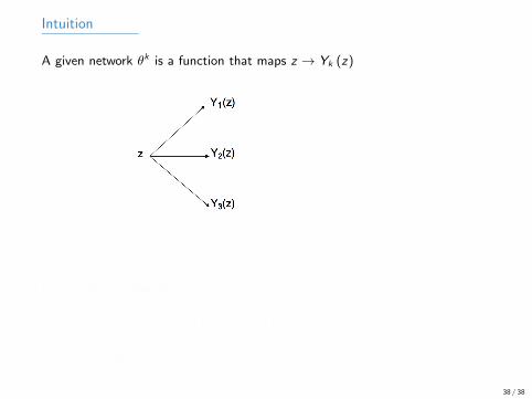
Intuition

A given network θk is a function that maps z → Yk (z)

From extreme value theory

Var (Y ) = Var

(max

k∈1,...,2nYk

)declines rapidly with n Return

38 / 38

cascades and fluctuations in an economy with an …

Documents