case study in ahmedabad - itc
TRANSCRIPT

Geo-spatial modeling for competition-based accessibility to job locations for the urban poor: case study in Ahmedabad
CHAO ZHEN February, 2013
SUPERVISORS:
Dr. ir. M.H.P. (Mark) Zuidgeest Dr. S. (Sherif) Amer


Thesis submitted to the Faculty of Geo-Information Science and Earth
Observation of the University of Twente in partial fulfillment of the
requirements for the degree of Master of Science in Geo-information Science
and Earth Observation.
Specialization: [Urban planning and management]
SUPERVISORS: Dr. ir. M.H.P. (Mark) Zuidgeest Dr. S. (Sherif) Amer
THESIS ASSESSMENT BOARD:
Prof. dr. ir. M.F.A.M. van Maarseveen (Chair)
Ing. K. M. van Zuilekom (External Examiner, University of Twente)
Geo-spatial modeling for competition-based accessibility to job locations for the urban poor: case study in Ahmedabad
CHAO ZHEN Enschede, The Netherlands, [February, 2013]

DISCLAIMER
This document describes work undertaken as part of a programme of study at the Faculty of Geo-Information Science and
Earth Observation of the University of Twente. All views and opinions expressed therein remain the sole responsibility of the
author, and do not necessarily represent those of the Faculty.

i
ABSTRACT
With rapid urbanization, there are more and more socially excluded people living in mega cities around the
world. Often, they can’t conveniently access some of the essential social activities like jobs, healthcare
services and so on because of the inadequate public transport or poorly transport planning. To solve the
problem of insufficient transport supply is not too hard but it definitely not easy to make a reasonable
planning scheme. Accessibility metrics can help planners to analyze where the socially excluded (in terms of
transport) are living in the urban area. As such it is one of most important indicators to quantify the
relationship between transport and land use. However, most accessibility measures used in practice ignore
some important factors such as the competition for opportunities, the potential of destinations etc. This
research provides a specific discussion about the drawbacks of some existing accessibility measures.
Cheng et al. (2012) proposed a competition-based model (i.e. Cheng’s model) to measure job accessibility
applied to Amsterdam, which considers travel cost, competition, diversity of jobs and a decay function.
Based on Cheng’s model, this research aimed to implement and adapt this model as an automation tool in
the ArcGIS 10.1 environment with Python and apply it for the specific case of accessibility to the urban poor.
This is done for Ahmedabad, India using the data from the World Bank project (Zuidgeest et al., 2012).
Meanwhile, this research considers the travel fare as an important factor that determines the level of job
accessibility of the urban poor. Using the provided 3D road network and Network Analyst tool, the Fare
tool is developed and programmed to calculate the monetary expenditure of each route. Finally, this research
analyzes and discusses the job accessibility for the urban poor in Ahmedabad with the fare and time decay
function respectively.
As a case study, this research evaluates the public transport of Ahmedabad in relation to a housing project
named SEWSH using the adapted and GIS-implemented version of Cheng’s model. According to Cheng’s
model, this research finds that providing one more public transport mode can’t enhance the job accessibility
of all worker locations in Ahmedabad because the accessibility analysis involves the competition factors.
One more travel mode such as the AMTS can help people to reach more employment locations comparing
to only walking. But the competition also increases at the employment location because of more workers.
Therefore, the method for interpreting the result of Cheng’s model is proposed by this research. Based on
the interpretation method, the results reveal that the AMTS (i.e. ordinary bus) is the most efficient travel
mode for the poor people who live in slums/chawl area. In contrast the BRTS (i.e. Bus Rapid Transit) and
MRTS (i.e. metro) only marginally contribute in the level of accessibility for these workers, which is not
surprising given the difference in the extent of both systems as compared to the AMTS. Once workers live
in SEWSH locations, most of their job accessibility increases. The BRTS and MRTS, moreover, further
improve the job accessibility for them. In addition, the time decay function has the better effect on the
improvement of job accessibility than that of fare decay function for the urban poor.
Key words: Job accessibility, Competition, Fare, Python, 3D road network, Decay function

ii
ACKNOWLEDGEMENTS
First, I want to thank the Faculty of Geo-Information Science and Earth Observation of the University of
Twente (ITC) and Chang’an University, because they provide this great opportunity for me to study in the
Netherlands. The abroad study and life are my precious wealth, which doesn’t only give me the rich
knowledge, but also enrich my experience and broaden my horizon.
My sincere appreciations belong to my supervisors Dr. Ir. M.H.P. Zuidgeest and Dr. S. Amer. There is no
doubt that I can’t finish my thesis successfully without their help. Their regular feedbacks and meetings
don’t only give me the academic suggestions, but also have the encouragement for me. I have gained lots of
useful knowledge from their patient and professional guidance.
I would like thanks to Ing. F.H.M.(Frans) van den Bosch, Talat Munsh, PhD Zhou Liang and Xiong Biao
very much. Frans provided to me the useful data, including the 3D multi-modal road network and other
relevant data. Without these data, it is impossible to finish my research. Talat Munsh gave me some
introductions about the Ahmedabad. The local knowledge is very useful for my research. Zhou Liang and
Xiong Biao helped me to figure out the programming ideas. They open my mind about how to design the
programming process.
To all my friends in ITC, I thank to you because it is happy to study with you. You don't only encourage me,
but also give me lots of helps when I’m in trouble. I can’t forget the period of time studying and living with
you in ITC.
My special thanks are for my parents and grandparents. You support me all the same time. Moreover, you
give me the trust, encouragement, spirit and material support, with which I can do anything confidently. If
the thesis were an award, half of its honour belongs to you. Without you, I can’t go abroad and can’t finish
my MSc study in the Netherlands. My love belongs to you forever.
Chao Zhen
February, 2013

iii
TABLE OF CONTENTS
List of figures ................................................................................................................................................iv
List of tables ...................................................................................................................................................v
List of Acronyms ........................................................................................................................................ vi
1. Introduction ...........................................................................................................................................1 1.1. Background .................................................................................................................................................... 1 1.2. Justification ..................................................................................................................................................... 1 1.3. Research problems ........................................................................................................................................ 2 1.4. Objectives ....................................................................................................................................................... 2 1.5. Research questions ........................................................................................................................................ 3 1.6. Conceptual framework ................................................................................................................................. 3 1.7. Research design ............................................................................................................................................. 5 1.8. Research matrix ............................................................................................................................................. 6 1.9. Research phases ............................................................................................................................................. 7 1.10. Structure of thesis ........................................................................................................................................ 8
2. Review of related accessibility measures ...........................................................................................9 2.1. Basic description of accessibility ................................................................................................................ 9 2.2. Cheng’s competition-based accessibility model .................................................................................... 10 2.3. Overview of commonly used accessibility measures .......................................................................... 11 2.4. Comparison between Cheng’s model and other accessibility measures ........................................... 15 2.5. Common problems of accessibility analysis ......................................................................................... 15
3. Study area and data ............................................................................................................................ 17 3.1. Overview of Ahmedabad ......................................................................................................................... 17 3.2. Housing for the urban poor ..................................................................................................................... 17 3.3. Jobs for the urban poor ............................................................................................................................ 19 3.4. Urban transport in Ahmedabad .............................................................................................................. 19
4. Implementation of Cheng’s Accessibility Model in ArcGIS ...................................................... 21 4.1. General description about implementation ........................................................................................... 21 4.2. Programming of the Fare tool ................................................................................................................ 22 4.3. Programming of the Competition tool.................................................................................................. 24 4.4. Interpretation of the results ..................................................................................................................... 28
5. Accessibility analysis and results ...................................................................................................... 31 5.1. Data preparation ........................................................................................................................................ 31 5.2. Explanation about research scenarios .................................................................................................... 36 5.3. Explanation about the Interpretation ..................................................................................................... 36 5.4. Accessibility results .................................................................................................................................... 38
6. Conclusions and Recommendations ............................................................................................... 51 6.1. Conclusion .................................................................................................................................................. 51 6.2. Recommendations ..................................................................................................................................... 52
List of references ........................................................................................................................................ 53
Appendice 1 Python codes of The Fare tool......................................................................................... 56
Appendice 2 Python codes of The Competition tool .......................................................................... 59

iv
LIST OF FIGURES
Figure 1 Conceptual framework ......................................................................................................................... 4
Figure 2 Research phases ..................................................................................................................................... 7
Figure 3 Example of Cheng’s model ............................................................................................................... 11
Figure 4 Example of 2SFCA ............................................................................................................................ 13
Figure 5 Road network and remote sensing image ........................................................................................ 16
Figure 6 Example of common problems for accessibility measures.......................................................... 16
Figure 7 Geographic location of Ahmedabad ............................................................................................... 17
Figure 8 Original Slum/Chawls and SEWSH locations ............................................................................... 18
Figure 9 Slums/Chawls and SEWSH in Ahmedabad ................................................................................... 19
Figure 10 Crowded main roads in Ahmedabad ............................................................................................. 20
Figure 11 2D and 3D road network ................................................................................................................. 20
Figure 12 Fare structure ..................................................................................................................................... 23
Figure 13 Comparison between the 2D result and the 3D result of Network Analyst .......................... 23
Figure 14 Example of Closest Facility ............................................................................................................ 24
Figure 15 Interface of the Fare tool ................................................................................................................ 24
Figure 16 Example of competition model ..................................................................................................... 25
Figure 17 Interface of the Competition tool .................................................................................................. 28
Figure 18 Aggregated number of jobs and workers ..................................................................................... 31
Figure 19 Time decay function ......................................................................................................................... 32
Figure 20 Fare decay function ........................................................................................................................... 33
Figure 21 Public transport systems in Ahmedabad ....................................................................................... 34
Figure 22 Intra-zone problem ........................................................................................................................... 34
Figure 23 Slums/Chawls and SEWSH locations after changing dwelling places ..................................... 35
Figure 24 Comparison job opportunities of only walking with that of walking and AMTS ................. 40
Figure 25 Comparison job opportunities of time decay with that of fare decay by all travel modes ... 42
Figure 26 Average job opportunities for three levels of poor people ........................................................ 43
Figure 27 Improvement of job accessibility for different poor classes with time decay function ........ 44
Figure 28 Percent of increased jobs for three levels of poor people ......................................................... 45
Figure 29 Improvement of job accessibility for three levels of poor people with fare decay function46
Figure 30 Comparison between SEWSH and remained Slums/Chawls .................................................... 48
Figure 31 Comparison between SEWSH and original Slums/Chawls ....................................................... 49

v
LIST OF TABLES
Table 1 Research matrix ....................................................................................................................................... 6
Table 2 Results of Network Analyst ............................................................................................................... 25
Table 3 Job opportunities when diversity and decay factor are 1 ............................................................... 26
Table 4 Final job opportunities ........................................................................................................................ 26
Table 5 Relations between the table fields and components of Cheng’s model ...................................... 27
Table 6 Job opportunities when diversity factor is 1 but the beta of decay function is 0.5 ................... 28
Table 7 Job opportunities when diversity factor is not 1 but decay factor is 1. ....................................... 29
Table 8 Job opportunities based on the improved road network ............................................................... 30
Table 9 Final job opportunities based on the improved road network ..................................................... 30
Table 10 Relationship between house and job type ...................................................................................... 32
Table 11 Properties of road network .............................................................................................................. 33
Table 12 Research scenario matrix .................................................................................................................. 36
Table 13 Explanation about abbreviations ..................................................................................................... 36
Table 14 Results of worker location 1421 by walking .................................................................................. 37
Table 15 Results of worker location 1421 by walking and AMTS ............................................................. 37
Table 16 Results of job location 369 by walking and AMTS ...................................................................... 37
Table 17 Comparison among W, WA and WABM for all worker locations.............................................. 39
Table 18 Number of increased job opportunities between different combinations of travel modes . 39
Table 19 Explanations about Figure 27 .......................................................................................................... 44
Table 20 Explanation about Table 21 ............................................................................................................. 45
Table 21 Improvement of job accessibility for three levels of poor people with fare decay function 45
Table 22 Percent of increased jobs for three levels of poor people .......................................................... 45
Table 23 Explanation about Figure 29 ............................................................................................................ 46

vi
LIST OF ACRONYMS
AMTS Ahmedabad Municipal Transport Service
BRTS Bus Rapid Transit System
MRTS Mass Rapid Transit System
SEWSH Socially and Economically Weaker Section Housing
ITC Faculty of Geo-Information Science and Earth Observation in Twente University
AMC Ahmedabad Municipal Corporation
CEPT Centre for Environment Planning and Technology University
AUDA Ahmedabad Urban Development Authority

GEO-SPATIAL MODELING FOR COMPETITION-BASED ACCESSIBILITY TO JOB LOCATIONS FOR THE URBAN POOR: CASE STUDY IN AHMEDABAD
1
1. INTRODUCTION
1.1. Background
During the recent decades, mega cities have come up around the world due to the fast growing urban
population. This rapid urbanization has led to social exclusion in many developing countries. The socially
excluded people “are not just poor, but that have additionally lost the ability to both literally and
metaphorically connect with many of the jobs, services, and facilities that they need to participate fully in
society”(Church et al., 2000, pg.197). Actually, the inadequate transport infrastructure mainly causes the
social exclusion because it reduces the convenience of access to public transport for the urban poor (Wati,
2009), for whom a private motorized mode is too expensive. Moreover, the public transport alternatives
are not planned for well enough.
Transport planning plays an important role in mitigating social exclusion in many cities. However,
traditional transport planning has an evident shortcoming as well. It only focuses on the efficiency of the
road network, while it ignores the interaction among people (e.g. competition among workers and
employers etc) and infrastructure (e.g. road network, transport hubs etc). This biased planning idea,
therefore, produces outcomes that don’t fit the aim of reaching a sustainable urban transport development.
Examples include the construction of a metro line for enhancing the accessibility of poor people, while
they can’t use it because of affordability problems, which is not considered or underestimated during the
planning phase. So integration of social-economic interaction with traditional transport methods can help
people to understand and plan transport systems better.
Low income people are living in the marginalized areas of cities such as Ahmedabad, India, and
experience high levels of social exclusion. The main reason is that they don’t have a good education
background or working skills, which forces them to just get the low payment jobs. Moreover, the
commuting expense of overcrowded public transport grows quickly due to the insufficient supply and
increasingly high demand. This is a critical social problem. If too many people can’t find a job for living,
the society would be unstable happening conflicts.
In order to help excluded poor people, many cities in India, like Ahmedabad, have started improving the
urban transport system to make the city more equitable and efficient. Meanwhile, the government tries to
integrate urban development and transport planning together in order to get better outcome. For example,
the government gives some priority policies for the urban poor to use the new constructed metro, bus
rapid transit and some other basic infrastructure. At the same time, several slum improvement programs
are being implemented such as the Basic Service to Urban Poor (BSUP) or Socially and Economically
Weaker Section Housing (SEWSH) program. These projects aim at preventing the poor people to be
excluded from the activities, which are the bases to improve their quality of life (Lucas, 2004).
1.2. Justification
Accessibility, which deal with measuring the convenience of people moving from one place to the other
place, could help planners to make a useful framework for the integration of transport and land use
planning (Bertolini et al., 2005). As Gutiérrez (2009) wrote, accessibility analysis enables one to identify
which areas are poorly covered or good served by the urban facilities. However, the existing accessibility
model is not good as the competition-based model proposed by (Cheng et al., 2012). (In the following

GEO-SPATIAL MODELING FOR COMPETITION-BASED ACCESSIBILITY TO JOB LOCATIONS FOR THE URBAN POOR: CASE STUDY IN AHMEDABAD
2
parts, Cheng’s model is the accessibility model from (Cheng et al., 2012)). That is because Cheng’s model
explicitly considers more factors, which are potential destinations, the diversity factors and the interaction
among people (i.e. the competition on demand and supply side) comparing to other accessibility measures.
The detailed comparison between Cheng’s model and other commonly used accessibility measures is
explained in the Chapter 2. Then, we can see that Cheng’s model is more realistic due to involving several
important factors, while the author didn’t provide a specific explanation about how to interpret the results.
Therefore, this research explores how Cheng’s model can be used and improved in the context of studying
accessibility for the urban poor in Ahmedabad. Meanwhile, the algorithms of Cheng’s model are
implemented in ArcGIS as a specialized tool. By this tool, it is easy to run various scenarios and use these
results to find a reasonable interpretation method, which can help planners to formulate schemes enhancing
accessibility for the urban poor.
1.3. Research problems
Ahmedabad is an upcoming mega city in India, where 25% of total population live in slums (Ahmedabad
Municipal Corporation et al., 2006). The city experiences quite a few problems caused by the poor
transport planning and management, in particular lack of infrastructure for pedestrians and cyclists as well
as congested traffic due to traffic behaviour and capacity problems of its roads. Moreover, the large
amount of poor people having a low income constrains them to access jobs because of the affordability
problems for public transport. Obviously, social exclusion, which is caused by the insufficient public
transport supply, doesn’t only reduce the number of job opportunities for the urban poor, but also heavily
limits Ahmedabad development.
To mitigate the high rate of social exclusion in the city, the local government planned to construct a Metro
system linking the current Ahmedabad Municipal Transport Service (AMTS) and the Bus Rapid Transit
System (BRTS). These programs are expected to impact on the travel behaviour of all people who live in
the city, including the urban poor. So the key question is how to adopt accessibility metrics to measure the
effect of these infrastructure projects on the ability of the urban poor to reach jobs and propose solutions
for the urban poor to get more benefits from these infrastructure projects.
In order to measure the improvement of job accessibility for the urban poor produced by these projects, this
research adapts Cheng’s model for Ahmedabad. However, as the pervious part mentioned, Cheng’s model
may not be completely suitable for the case of Ahmedabad because this mode before was used to measure
accessibility of workers in Amsterdam where has the different social-economic background compare to
Ahmedabad. Therefore, Cheng’ mode needs to be adapted. Then, Cheng’s model is complemented with the
inclusion of generalized cost (i.e. fare and travel time impedances) as the urban poor are expected to value
fares very much because of their relatively low income. Finally, we interpret the results to guide policy
making for sustainable transport planning.
1.4. Objectives
1. General objectives
1) To adapt and implement the accessibility model proposed by (Cheng et al., 2012) for the study of job
accessibility of the urban poor in Ahmedabad.
2. Sub-objectives
1) Assess Cheng’s accessibility model for its possible use in Ahmedabad
2) Adapt and improve Cheng’s accessibility model for the urban poor in Ahmedabad.
3) Implement Cheng’s accessibility model in the ArcGIS environment.
4) Investigate the implications of Cheng’s accessibility model for the urban poor.

GEO-SPATIAL MODELING FOR COMPETITION-BASED ACCESSIBILITY TO JOB LOCATIONS FOR THE URBAN POOR: CASE STUDY IN AHMEDABAD
3
1.5. Research questions
These research questions related to the four sub-objectives are: Sub-objective (1): assess Cheng’s accessibility model for its possible use in Ahmedabad
1) How does Cheng’s accessibility models work and compare to other such models?
2) What are the innovative points of Cheng’s accessibility model?
3) What are the shortcomings of Cheng’s accessibility models?
Sub-objective (2): adapt and improve Cheng’s accessibility model for the urban poor in
Ahmedabad.
4) How does the model involve the generalized cost (i.e. the fare and travel time impedance)?
5) What’s the relationship between different types of urban poor and different jobs?
6) What are the related parameters of adapted Cheng’s model? Sub-objective (3): implement Cheng’s accessibility model in the ArcGIS environment.
7) What are the key functions in ArcGIS to implement this model?
8) What are the limitations of ArcGIS to implement this model?
9) Which approach can solve these limitations?
10) What is the sequence of implementation?
Sub-objective (4): investigate the implications of Cheng’s accessibility model for the urban poor.
11) How does the result evaluate the effect of infrastructure projects for the urban poor in Ahmedabad?
12) Which class of urban poor could have the lowest accessibility to job locations?
13) Which type of transport project is the most useful and convenient for the urban poor?
14) Which combination of travel modes is the most efficient way to increase the job accessibility for the
urban poor in Ahmedabad?
1.6. Conceptual framework
The conceptual framework involves three parts, and concern the demand part (i.e. workers/the urban
poor), the supply part (i.e. employers) and the physical infrastructure (i.e. public transport). These factors
affect on job accessibility of the urban poor.
All of the factors are influenced by the urban form. As Lynch (1981) defined, urban form is the spatial
arrangement of human activities, which produces spatial flows of persons, goods as well as information.
Meanwhile, these social activities change the public facilities and people’s decisions, which shape and
modify the urban form. It means the spatial locations of the demand, supply and physical infrastructure
are somehow determined by the urban form and there is also mutual influence between each other. Due
to the different spatial distribution of demand and supply, people have to use the physical infrastructure to
overcome the friction of distance. So transport mainly impacts on accessibility, which is the most important
link between the demand and supply side.
Specifically, in this research, the characteristics of demand and supply are determined by the interaction of
people (i.e. the competition factors) and the competition is influenced by the living environment, the
character of jobs, the number of workers and jobs. For example, some people are willing to go further
looking for a job because of the low competition and high salary etc. Then, their behaviours alter the
intensity of competition of a certain job market. Obviously, these characteristics of demand and supply
consist of the social-economic interaction, which should be one of the key elements of accessibility.
In terms of physical infrastructure, the fare, frequency, speed, categories and transfer of public transport
are significant attributes for job accessibility of the urban poor. And these factors react the efficiency of
the public transport and how difficult to access to this system.

GEO-SPATIAL MODELING FOR COMPETITION-BASED ACCESSIBILITY TO JOB LOCATIONS FOR THE URBAN POOR: CASE STUDY IN AHMEDABAD
4
Figure 1 Conceptual framework
Urban form
Social-economic interaction
Physical infrastructure (Public transport)
Fare
Frequency
Speed
Categories
Transfer
Demand
(The urban poor)
Competition
Number of workers
Living environment
Supply
(Employers)
Competition
Number of jobs
Job character
Job accessibility

GEO-SPATIAL MODELING FOR COMPETITION-BASED ACCESSIBILITY TO JOB LOCATIONS FOR THE URBAN POOR: CASE STUDY IN AHMEDABAD
5
1.7. Research design
1.7.1. Research data
The data has been obtained from a World Bank project executed by ITC and CEPT University in
Ahmedabad (Zuidgeest et al., 2012). Data used in this research is therefore limited to those data collected
in that project. The focus is on the evaluation, implementation and interpretation of Cheng’s model.
1.7.2. Research methods
1. Modelling accessibility and its components
The method is to adapt the main components of Cheng’s model for Ahmedabad. The most important
components of Cheng’s model are travel cost, diversity factor, decay function and competition factors. For
travel cost, the time impedance can be gotten from Network Analyst from ArcGIS 10.1 based on the 3D
road network, while the fare requires the combination of related functions of ArcGIS to calculate, which is
explained specifically in section 4.2. Moreover, Cheng’s model doesn’t consider the fare as a factor to
influence accessibility but this research incorporates the fare into accessibility analysis. Then, the diversity
function, decay function and competition factors are directly used from Cheng’s model. But the beta
parameter of decay function is calibrated by the related reports or literature about the travel behaviour of the
urban poor in Ahmedabad.
2. Implementation method
1) Geoprocessing tools
ArcGIS has a package of powerful geoprocessing tools, which has hundreds of functions to deal with
geographic data analysis. These functions can help researchers to know the spatial characters of urban
development. Moreover, the Network Analyst function is the key method to know the efficiency of
transport infrastructure. So this research adopts these tools to implement Cheng’s mode in ArcGIS.
2) Python scripting
Even though it is feasible to work out the accessibility of Cheng’s model by these geoprocessing tools, the
computing processes are complicated and the speed is slow because of the ways of data storage structure and
data reading by geoprocessing tools. In contrast, Python provides a good data management and calculation
environment. And ArcGIS provides a module for Python scripting named Arcpy, which can combine
geoprocessing tools with Python. So this research adopts Python to execute the core calculations and
encapsulate related geoprocessing functions as a specialized tool for Cheng’s model. And this specialized
tool implements the algorithms of Cheng’s model in the ArcGIS environment.
3. Interpretation method
This method includes statistical analysis and visualization methods to evaluate job accessibility, transport
projects in Ahmedabad. And it is a way to explore how to use this accessibility model in urban planning.

GEO-SPATIAL MODELING FOR COMPETITION-BASED ACCESSIBILITY TO JOB LOCATIONS FOR THE URBAN POOR: CASE STUDY IN AHMEDABAD
6
1.8. Research matrix
Data requirement Model methods Answered questions
Implementation methods
Answered questions
Interpretation method
Answered questions
Urban poor
Slum level
The decay function Competition formulas
Questions 1), 2), 3), 4), 5), 6)
Geoprocessing tools
Python script
Questions 4),7), 8), 9), 10)
Statistical methods Visualized methods
11), 12), 13, 14)
Spatial location
The number of workers
Jobs
Job types
Spatial location
The number of jobs
Public transport network dataset
Fare
3D multi-modal road network dataset
Questions 4), 7), 8), 10)
Speed
Transfer
Frequency
Table 1 Research matrix

GEO-SPATIAL MODELING FOR COMPETITION-BASED ACCESSIBILITY TO JOB LOCATIONS FOR THE URBAN POOR: CASE STUDY IN AHMEDABAD
7
1.9. Research phases
In order to achieve the research objectives, there are four major phases to be done.
1) The first phase is to assess the popular accessibility models, have an overview of the data and
Ahmedabad. The strengths and weaknesses of Cheng’s model can be found after the evaluation of
other relevant accessibility models. The overview of data and Ahmedabad is the preparation for
adapting Cheng’s model.
2) The second phase aims at making Cheng’s model fit for Ahmedabad. Specifically, the major
components of Cheng’s model (i.e. the diversity factor, the definition of the decay and competition
function) are adapted for Ahmedabad. And the parameters of the decay and competition function are
calibrated according to the context of Ahmedabad.
3) In the third phase, the algorithms of Cheng’s model are implemented as a specialized tool in ArcGIS,
which combines the geoprocessing functions with Python.
4) The fourth phase runs the accessibility tool developed by this research to analyze the job accessibility
of the urban poor in Ahmedabad based on different research scenarios. And then the interpretation
method is discussed and formulated to evaluate the transport and housing projects in Ahmedabad.
Meanwhile, this research concludes how to use Cheng’s model in urban planning.
Figure 2 Research phases
Assess existing models
Implement the algorithms of Cheng’s model in ArcGIS
Phase 1
Phase 2
Phase 3
Overview of Ahmedabad Basic data analysis
Generally definite research methods
The adapted Cheng’s model for Ahmedabad
Evaluate the transport and housing projects.
Explain how to use the results in urban planning
Define diversity factor Define decay function Define competition
Geoprocessing functions Python script
Interpretation methods Phase 4
Formulate research scenarios
Job accessibility

GEO-SPATIAL MODELING FOR COMPETITION-BASED ACCESSIBILITY TO JOB LOCATIONS FOR THE URBAN POOR: CASE STUDY IN AHMEDABAD
8
1.10. Structure of thesis
This thesis includes six chapters. Below is a brief description of each chapter.
Chapter One: Introduction
This introductory chapter shows the background, research problems, objectives with the corresponding
questions and research design etc.
Chapter Two: Review of related accessibility measures
Description of existing accessibility models and concepts, which are relevant for this thesis, are discussed.
And there will be some specific arguments on the strength and weakness of these models.
Chapter Three: Study area and data
In this chapter, it provides the insight into the study area according to literature and includes a general
description about the data used in this research.
Chapter Four: Implementation of Cheng’s accessibility model in ArcGIS
This chapter specifies how to implement Cheng’s model in ArcGIS. It displays how to use Python
building Cheng’s model in ArcGIS as an automation tool.
Chapter Five: Accessibility analysis and results
The contents of this chapter are about how to make Cheng’s model adapt for the study area. Then, the
result of job accessibility in Ahmedabad is discussed based on different research scenarios. And the
interpretation method is formulated to evaluate the public transport and housing projects in Ahmedabad.
Chapter Six: Conclusions and Recommendations
This chapter provides some suggestions on how to use Cheng’s accessibility model in urban planning.
And according to the limitations of this research, there are also some recommendations for the further
study.

GEO-SPATIAL MODELING FOR COMPETITION-BASED ACCESSIBILITY TO JOB LOCATIONS FOR THE URBAN POOR: CASE STUDY IN AHMEDABAD
9
2. REVIEW OF RELATED ACCESSIBILITY MEASURES
This chapter has five sections. The first section provides a basic description of the accessibility concept,
which includes the definition, importance and components of accessibility. Second, Cheng’s model is
explained, especially for the competition factors. Third, it reviews and evaluates some related accessibility
measures, including the primary measures and the competition-based measures. Fourth, the comparison
between Cheng’s model and other accessibility measures is provided. The fifth section discusses about the
common problems of accessibility analysis.
2.1. Basic description of accessibility
2.1.1. Definition of accessibility
In a scientific forum, Hansen (1959) defined accessibility as “the potential of opportunities for interaction”.
From then on, there had been many different definitions about accessibility. Accessibility is “a property of
individuals and space which is independent of actual trip making and which measures the potential or
opportunity to travel to selected activities” (Morris et al., 1979, pg.92). And Geurs and van Wee (2004,
pg.128) consider accessibility as “the extent to which the land-use transport system enables (groups of)
individuals or goods to reach activities or destinations by means of a (combination of) transport mode(s).”
Accessibility can also be described as “the opportunities available to individuals and companies to reach
those places in which they carry out their activities” (Gutiérrez, 2009, pg.410). Actually, these definitions
are based on their researches but the core ideas are the same, which is to analyze the ease of access to
activities. For this research, accessibility means the urban poor by public transport can get how many jobs
when there is competition on the employer side and worker side.
Although the above definitions of accessibility don’t include keywords like social and economic, absolutely,
accessibility can’t separate from these three words. The main parts of accessibility like travelling, opportunity
or activity are strongly related to social-economic factors. For example, if researchers neglect the
social-economic factors in job accessibility analysis, the results could be biased. In some residential locations,
people can reach many job locations within a very short travel time, which means their accessibility is very
high. Actually, the real job accessibility is quite low because of the high intensity of competition. So we
should not only analyze the efficiency of infrastructure system (i.e. road network & public transport) in
accessibility analysis. But unfortunately, Moseley (1978) found most of accessibility analysis paid more
attention to physical analysis such as the spatial patterns, efficiency of public transport rather than
social-economic factors.
2.1.2. Importance of accessibility
This research agrees that “accessibility is an important spatial characteristic and an significant link between
transportation and land-use”(Hansen, 2009, pg.385). The mutual affect between land-use and transport
infrastructure is via accessibility. Specifically, land-use pattern determines the locations of activities and
residents. And the travel impedance (e.g. travel time/distance) depends on the efficiency of the transport
system. The government or transport department, therefore, often improves the certain links of road
network in order to increase the accessibility of some residential area. But after making transport better for
some sites, residents are likely to sell the lands to businessmen for other different activities due to the high
accessibility.

GEO-SPATIAL MODELING FOR COMPETITION-BASED ACCESSIBILITY TO JOB LOCATIONS FOR THE URBAN POOR: CASE STUDY IN AHMEDABAD
10
Accessibility, which is strongly related to social and economic factors, is a powerful tool or framework in
urban planning (Gutiérrez, 2009; Straatemeier, 2008). Thus it helps planners to know the urban status quo
and plan the future development well. For instance, in case of inequitable distribution like healthcare,
planners have used different accessibility models to understand the reasons of inequity and optimize the
healthcare source to achieve equity (Higgs, 2004). With regard to the economic aspect, land with high
accessibility is more worthy such as the land in the urban centre.
2.1.3. Components of accessibility
Depending on the different definitions of accessibility, researchers proposed various accessibility models,
while this research studies the model inclusion of the following three basic components, which are origins,
destinations (as in opportunity locations) and transport (as in travel impedance).
1) Origins are often residential areas, mostly represented as point locations or zonal polygons. The
number of origins in study area is influenced by the analysis scale a lot. If we want to calculate the
accessibility at the level of individual, a point represents one person. And when the analysis scale is
bigger not the level of individual, researchers often aggregate some places as one point like every street
block being an origin. So the accessibility of every person requires more origins than the aggregated
level of analysis.
2) Destinations, in which people carry out activities, can be different facilities (e.g. healthcare, job
location, school etc), also represented as point locations. The other specification is the same as that of
origin.
3) The transport refers to the generalized travel cost of different types of travel modes like car, metro,
bicycle etc. Hence, the simulation of the road network is the key part for measuring accessibility.
However, sometimes researchers don’t use road network to get travel cost, while they adopt a
Euclidean distance as the cost, although the straight distance is not close to reality. The Euclidean
distance is simpler and more efficient for calculation compare to road network. And the straight lines
are often used when the study area doesn’t have developed road network or it is flat area. For
building road network, there are two common approaches, which are vector-based and raster-based
network. For vector method, it is hard to simulate walking because people don’t only follow the road
network to walk. By contrast, the raster-based approach can create spatially continuous accessibility
surfaces (Hansen, 2009), which easily handles the walking simulation and deals with the road network
without complete data (Ahlstrom et al., 2011).
2.2. Cheng’s competition-based accessibility model
Actually, this research adopts the competition-based accessibility model from (Cheng et al., 2012) (i.e.
Cheng’s model). The detailed formulas are shown as follow:
𝐷𝑗 = − 𝑄𝑙𝑗 ×𝑙𝑛 (𝑄𝑙𝑗 )𝑙
ln (n), 𝑄𝑙𝑗 =
𝐸𝑙𝑗
𝐸𝑗 (1)
𝑓(𝑡𝑘𝑗 ) = e−𝛽×𝑡𝑘𝑗 (2)
𝑃𝑗𝑘 =𝐸𝑗
𝐷𝑗 ×𝑓(𝑡𝑘𝑗 )
𝐸𝑠𝐷𝑠×𝑓(𝑡𝑘𝑠 )𝑠
(3)
𝑄𝑖 = 𝐸𝑗 ×𝑃𝑗𝑖 ×𝑊𝑖×𝑓(𝑡𝑖𝑗 )𝑗
𝑃𝑗𝑘 ×𝑊𝑘×𝑓(𝑡𝑘𝑗 )𝑘 (4)
Eq. (1) is to define the diversity of jobs at location 𝑗, which is derived from the entropy, 𝐸𝑙𝑗 is the number of
𝑙 type jobs and 𝐸𝑙𝑗 is the total number of jobs at location 𝑗, 𝑛 is the number of job types.

GEO-SPATIAL MODELING FOR COMPETITION-BASED ACCESSIBILITY TO JOB LOCATIONS FOR THE URBAN POOR: CASE STUDY IN AHMEDABAD
11
Figure 3 Example of Cheng’s model
Eq. (2) is a negative exponential function for distance decay. 𝑡𝑘𝑗 is the travel time from residential location
𝑘 to employment location 𝑗. 𝛽 is a calibration parameter.
Eq. (3) represents the competition of employers for workers between location 𝑗 and 𝑠. 𝐸𝑗 is the total
number of jobs at location 𝑗. 𝐸𝑠 is the total number of jobs of all job locations. 𝐷𝑗 and 𝐷𝑠 are the diversity
of jobs in location 𝑗 and 𝑠 respectively.
Eq. (4) is the final job opportunity 𝑄𝑖 allocated to residential location 𝑖. W𝑖 and W𝑘 are the number of
workers at location 𝑖 and 𝑘 respectively, competing for jobs at location 𝑖.
The basic components of Cheng’s model are still the origins,
destinations and transport but this model mainly defines the interaction
among origins and destinations (i.e. two-side competition). According
to the Oxford Dictionary, the word “competition” has two explanations.
One is “a situation in which people or organizations compete with each
other for something that not everyone can have.” The other is “an event
in which people competes with each other to find out who is the best at
something.” The competition factors of Cheng’s model match the two
definitions. Figure 3 is to explain the concrete calculations of two-side
competition (i.e. Eq. (3) and (4)), which doesn’t consider the diversity of
jobs and decay function of Cheng’s model in order to show the major
calculations clearly. In Figure 3, the arrow direction is competition
direction. Location B is so far away from job location C that no one from B finds a job in C. Then, the
competition for worker location A between employers of C and D are 20/80=1/4 and 60/80=3/4
respectively. This calculation fits the second definition of competition in Oxford Dictionary (i.e. “an event in
which people competes with each other to find out who is the best at something.”). That is to compare
which job location is better or more attractive. So the competition among employers can also be regarded as
the attractiveness of a job location. For the competition among workers, the calculation follows the first
definition of competition (i.e. “a situation in which people or organizations compete with each other for
something that not everyone can have.”). The competition among workers of A and B for jobs D is 60/(100
x 3/4+50) = 0.48. In other word, when workers from A or B look for jobs in D, everyone can get 0.48 jobs
from statistical view. And 75 people from A will go to D for jobs because 100 x 3/4 =75 (i.e. the number of
people from A multiplies the competition factors among employers). Likewise, 25 people from A will go to
C and 50 people from B go to D. Finally, the accessibility of A is 0.48 x 75 +20 =56 and the result of B is 0.48
x 50 =24. It means that workers of A and B can get 56 and 24 jobs respectively. The job accessibility of A is
higher than the accessibility of B.
2.3. Overview of commonly used accessibility measures
In order to compare Cheng’s model to other accessibility models, the following sections review of some
popular accessibility measures, which are related to Cheng’s model.
2.3.1. Infrastructure-based measure
This method focuses on the efficiency of the road network, in which the locations of origins and
destinations are required but other characteristics from origins and destinations are ignored. This measure
requires data about physical infrastructure like the bus lines, cycling lanes and waiting time for public
transport etc. With this kind of data, this method can, for example, reflect the congestion level and help
researchers to find the most efficient transport corridor. So the infrastructure-based measure is easy to
calculate and interpret. Yet, it lacks of the social-economic factors involved.

GEO-SPATIAL MODELING FOR COMPETITION-BASED ACCESSIBILITY TO JOB LOCATIONS FOR THE URBAN POOR: CASE STUDY IN AHMEDABAD
12
2.3.2. Cumulative measure
The contour or isochrones measure (Geurs & van Wee, 2004) (also called threshold measure) is frequently
used in urban planning. The first step of this measure is to count the total number of reachable destinations
in a certain travel distance or time from an origin by the possible transport modes (Lovett et al., 2002). Then,
the total number of opportunities from every reachable destination for one origin is calculated. Here the
origins and destinations are more important, especially the number of opportunities from destinations.
For example, residents from A can reach 2 healthcare units via the fastest travel mode in 15 minutes and
each healthcare unit has 3 practitioners, while people living in B can reach one healthcare unit by the same
mode in 15 minutes and this healthcare unit has 7 practitioners. Consequently, residents of A and B can
get 6 and 7 practitioners in 15 minutes respectively. We can say the accessibility of B to healthcare is
higher than that of A in 15 minutes. In terms of transport component of this measure, the road network is
not necessary because researchers can use Euclidean distance to represent the travel impedance.
This paragraph discusses about the strengths and weaknesses of cumulative measure. The strength of the
cumulative measure is easy to calculate and interpret because it only counts the number of opportunities
available for every origin. Moreover, the cumulative measure considers the character of destinations (i.e.
the number of opportunities) comparing to the infrastructure-based measure. And the visualization is
intuitive and meaningful. One of the major problems for cumulative measure is to give every destination
equal weight in a certain travel distance or time threshold and it doesn’t consider the opportunities outside of
this threshold. Like the example of above paragraph, if there is another healthcare unit with 2 doctors away
from A 16 minutes, which is a little more than defined time threshold (i.e. 15 minutes). In reality, people of
A could get service from this 16-minute healthcare. Therefore, it is not exact that the accessibility of B to
healthcare is higher than that of A.
2.3.3. Potential measure
The potential accessibility measure assigns the different weight for each destination depending on a
distance decay function, which means the accessibility level of one origin is inversely proportional to the
distance away from destinations. Obviously, the origins and destinations are also important. Like the
cumulative measure, the number of opportunities of each destination is key factor to influence the final
accessibility. For the transport part, it can be road network or Euclidean distance. And the common
formula is demonstrated below:
𝐴𝑖 = 𝐷𝑗𝑓(𝑐𝑖𝑗 )𝑛
𝑗=1 (5)
𝑓(𝑐𝑖𝑗 ) = 𝑒−𝛽𝑐𝑖𝑗 (6)
Where 𝐴𝑖 is the accessibility of origin 𝑖, 𝐷𝑗 is the total number of facilities or opportunities at location 𝑗,
𝑓 𝑐𝑖𝑗 is the general decay form and it can be power function, combination of power function with
negative exponential function and so on, Although the decay function has many forms, most of researchers has chosen the negative exponential function because it is closer to people’s travel behaviour (Handy &
Niemeier, 1997). So the most common used decay function is 𝑒−𝛽𝑐𝑖𝑗 , 𝛽 is a calibration parameter, 𝑐𝑖𝑗 is
the travel impedance (e.g. travel distance or time) from 𝑖 to 𝑗.
In terms of the advantages and disadvantages of the potential measure, one of this method’s advantages is to
consider the opportunities of all destinations. The travel time can’t limit the reachable destinations but the
time can discount the opportunities from the destination. Another advantage is easy to calculate and
interpret because it is to measure the probability of available opportunities from each destination for every
origin. And the visualization is very simple. For the disadvantage, it is not easy to define the decay function
because everyone has the different travel behaviours. Even though the negative exponential function is
GEO-SPATIAL MODELING FOR COMPETITION-BASED ACCESSIBILITY TO JOB LOCATIONS FOR THE URBAN POOR: CASE STUDY IN AHMEDABAD
13
often used, sometimes the beta parameter is not meaningful in the function. For example, the travel time 30
minutes is equal to 0.5 hour, while it is evident that 𝑒−𝛽∙30 ≠ 𝑒−𝛽∙0.5. This example also proves that this
kind of distance decay function is very sensitive to the unit of travel time.
2.3.4. Competition-based measure
Besides above primary measures, some researchers tried to incorporate the competition factor into
accessibility model (for example, (Joseph & Bantock, 1982; Joseph & Philips, 1984; Weibull, 1976; Wilson,
1971)). Generally speaking, there are two categories of competition-based measures. One is constituted by a
competition factor and decay function like Two-step Floating Catchment Area. This category always
involves one side of competition. The other kind of competition-based measure is Singly/Doubly
Constrained Gravity Model, which can simulate one or two sides of competition. Both of measures mainly
study how the intensity of competition influences the accessibility. Comparing to primary measures, the
competition-based measure is more realistic. However, it is not easy to interpret the results due to the
competition factor involved. The following sections illustrate two most popular competition-based
measures, which are (Two-step) Floating Catchment Area and Singly/Doubly Constrained Gravity Model.
1) Two -step Floating Catchment Area
The original version of this measure was to calculate the job to housing ratio (i.e. service or opportunities)
(Peng, 1997), which can be considered as the intensity of competition on the demand side (i.e. the number of
facilities or opportunities available for everyone). The centroid of the Floating Catchment Area (FCA) is the
demand location (i.e. origin). And the FCA overcomes the drawback of fixed analysis zones, which is in
other accessibility measures. Specifically, without FCA, researchers divide the study area into several zones,
which are often partitioned by administrative boundaries or traffic analysis zones. This zoning method is
criticized neglecting the cross boundary issue. For example, although people (i.e. demand) don’t only look
for a job (i.e. supply) in the analyzed area (e.g. traffic analysis zone or administrative district), researchers
assume that people can only get the employment opportunities in one fixed zone. Obviously, they could go
outside of the analyzed zone finding jobs. Thus, the FCA provides different catchment areas for every
demand location depending on its character to solve the cross boundary problem. The results of FCA are
opportunities to people ratios, which mean how many opportunities are gotten by everybody in the
catchment area. Consequently, this model only takes account into competition on the demand side.
Following the FCA method, Radke and Mu (2000) proposed Two-step Floating Catchment Area (2SFCA),
which was explained how to implement in ArcGIS by (Wang & Luo, 2005). There are two steps for
calculation in the 2SFCA, which is to do the floating catchment area twice with a different centroid. The first
computing centroid is supply location (i.e. destination). And then the demand side (i.e. origin) is chosen as
the centre. Comparing to FCA, the 2SFCA considers the character of the supply side because it makes the
supply as the centroid of catchment area to analyze the accessibility. Consequently, the two catchment areas
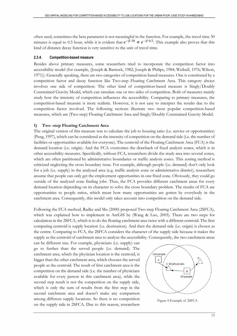
can be different size. For example, physicians (i.e. supply) can
go to further than the served people (i.e. demand). The
catchment area, which the physician location is the centroid, is
bigger than the other catchment area, which chooses the served
people as the centroid. The result of first catchment area is the
competition on the demand side (i.e. the number of physicians
available for every person in this catchment area), while the
second step result is not the competition on the supply side,
which is only the sum of results from the first step in the
second catchment area and doesn’t make any comparison
among different supply locations. So there is no competition
on the supply side in 2SFCA. Due to this reason, researchers Figure 4 Example of 2SFCA

GEO-SPATIAL MODELING FOR COMPETITION-BASED ACCESSIBILITY TO JOB LOCATIONS FOR THE URBAN POOR: CASE STUDY IN AHMEDABAD
14
frequently use the 2SFCA to measure the accessibility to healthcare. Obviously, they assume that there is
competition among people but no competition among the healthcares.
Figure 4 is an example of healthcare accessibility analysis by the 2FSCA. The location C has 80 physicians. In
a certain travel time, 100 people from A and 80 people from B can reach location C to get the healthcare
service. The ratio of physician to people at location C is 80/(100+60)=0.5 based on the algorithm of 2FSCA.
It means every one can get 0.5 physicians in this catchment area from mathematical view. And this
calculation fits the first definition from Oxford Dictionary (i.e. “a situation in which people or organizations
compete with each other for something that not everyone can have.”). Subsequently, using the same method
calculates a ratio for location D, which is assumed to be 0.8. Finally, the residential location B is chosen as
the centroid of the dashed catchment area within a threshold of travel time. So the accessibility of B is 1.3 (i.e.
0.5+0.8). This result is the average number of physicians available for everybody from location B.
This method also has some strengths and weaknesses. As the previous paragraphs mentioned, the strength
of the 2SFCA is to involve one-side competition and overcome the cross boundary problem. Moreover, the
result is easy to interpret, which reflects the number of opportunities available for every person. In terms of
the weaknesses, the original 2SFCA has two limitations. First, the results are very sensitive to the size of
catchment area because it assumes that people only can reach some facilities or get opportunities in the
catchment area. Second, it is lack of competition on the supply side. The first limitation can be solved by a
predefined the threshold or studying people’s travel behaviour. For example, Luo and Whippo (2012)
proposed a method to define a base value for population to get the reasonable catchment size. However, no
one gave a method to add competition on the supply side.
2) Singly/Doubly Constrained Gravity Model
This measure, which is derived from Newton’s law of gravitation, considers the characters of two sides (i.e.
the number of people and opportunities from origins and destinations respectively). The origins and
destinations are very important in the gravity measure and the travel cost is like potential measure, which can
be Euclidean distance or the result from road network analysis. The formulas are shown below:
T𝑖𝑗 = a𝑖b𝑗 O𝑖α𝑖D
𝑗
β𝑗𝑓(𝑐𝑖𝑗 ) (7)
ai = bjDjf(cij )nj=1
−1 (8)
bj = aiOif(cij )mi=1
−1 (9)
Where T𝑖𝑗 is the travel flow from 𝑖 to 𝑗, O𝑖 is the number of activities at location 𝑖 (e.g. the number of
people) and it reflects the willingness or desire to go somewhere, D𝑗 is the attractiveness of location 𝑗 and it
is often the number of activities or opportunities (e.g. the number of shops or jobs), α𝑖 and β𝑗 are the
calibration parameters. In many versions of gravity model, we assume α𝑖 = β𝑗 = 1 (Giuseppe Bruno &
Improta, 2008). The travel impedance between 𝑖 and 𝑗 is 𝑐𝑖𝑗 .
The formulas are the Doubly Constrained Gravity Model, while the Singly Constrained Gravity Model needs
to remove ai or bj depending on the modelling requirements. Some researchers thought this kind of gravity
model fit for measuring accessibility (for example, Fotheringham (1986), Horner (2004)). When the number
of people of each origin and the number of opportunities of every destination are fixed, we can use the
Doubly Constrained Gravity Model. Like measuring job accessibility, workers (i.e. origin) compete for jobs
(i.e. destinations) and employers compete for workers. So this case is good to use the doubly constrained
model. For shopping accessibility, only the number of residents is fixed because we assume that there is no

GEO-SPATIAL MODELING FOR COMPETITION-BASED ACCESSIBILITY TO JOB LOCATIONS FOR THE URBAN POOR: CASE STUDY IN AHMEDABAD
15
upper limitation for the shop’s capacity. In other words, the more customers patronize, the better operating
condition is. In this case, the Singly Constrained Gravity Model is adopted to measure the accessibility.
For the strengths and shortcomings of the gravity model, the strength is to consider the competition factors
on the origin side and destination side, which makes the analysis more realistic. However, the shortcoming
of the gravity measure is the complex and meaningless iterations. In some researches, there are hundreds of
origins and destinations, which make the balancing process complex. Because it can cost lots of time to
calculate in the computer. And the final results are not easy to interpret due to the iterative balancing process
just being a mathematic operation, which doesn’t have any real meanings and the calculation doesn’t fit the
two definitions of competition from the Oxford dictionary.
2.4. Comparison between Cheng’s model and other accessibility measures
Comparing to other measures except the competition-based measures (i.e. Singly/Doubly Constrained
Gravity Model and 2SFCA), Cheng’s model is more realistic and reliable due to including the two-side
competition, the diversity and decay function.
In terms of the comparison between Cheng’s model and the other two competition-based models
mentioned in section 2.3.4. First, Cheng’s model involves the two-side competition comparing to the
2SFCA which only includes one-side competition. And the result of Cheng’s model is the number of
opportunities for each origin, while the result of 2SFCA is a relative value, which is the average number of
opportunities for every origin. Second, Cheng’s model has the transparent definition and calculation
contrast with Singly /Doubly Constrained Gravity Model. Even though both models can include two
sides of competition, it is obvious that Cheng’s model avoids the meaningless iteration and has the clear
definitions about the competition as section 2.2 explained. Third, Cheng’s model is like a platform, which
is flexible to change. Every function of this model can be adjusted according to research requirements. It
is also easy to add new factors or parameters in Cheng’s model. Like this research, it focuses on the urban
poor in Ahmedabad, India. So the fare factor is incorporated into Cheng’s model.
However, the calculation of Cheng’s model costs more time due to more factors involved comparing to
other accessibility measures. This research implements Cheng’s model in ArcGIS to be an automation tool,
which can make the calculation more convenient. For the decay function, Cheng’s model uses the negative
exponential function. As section 2.3.3 explained, this kind of decay function sometimes is meaningless (e.g.
30 minutes = 0.5 hours but 𝑒−𝛽∙30 ≠ 𝑒−𝛽∙0.5). But this problem can’t be solved by this research. Another
major limitation of Cheng’s model is how to interpret because it involves several factors, which makes the
interpretation of Cheng’s model not as easy as other accessibility models, especially not like the models
without competition factors. This is an important problem to be solved by this research.
2.5. Common problems of accessibility analysis
There are two common problems for all accessibility measures, which are somehow solved by this research.
First, sometimes the results are often biased from the reality because of incomplete road network. The left
picture of Figure 6 shows people from residential location can take a bus or drive a car on the road going to
the shopping mall. Yet, there could be off-road path (i.e. the dashed lines in Figure 6), which costs less time
than the road path. Although this problem can’t be solved, this research mitigates this kind of problem by
the complete 3D multi-modal road network as Figure 5 shows.

GEO-SPATIAL MODELING FOR COMPETITION-BASED ACCESSIBILITY TO JOB LOCATIONS FOR THE URBAN POOR: CASE STUDY IN AHMEDABAD
16
Figure 5 Road network and remote sensing image
Second, the intra-zone problem is shown in the right side of Figure 6. If the analysis is regional or national
level, it is necessary to divide the study area into several zones in order to make sure the computer work out
results. No matter which kinds of accessibility measures, origins and destinations are points, which
frequently represents all of residents or opportunities in one analysis zone. The residential location (i.e.
origin) in Figure 6 represents all the people in zone A. Thus, the final accessibility of everybody in A is the
same as the accessibility of that point (i.e. origin), which is obviously not practical. The intra-zone problem is
caused by the predefined boundaries, which aims at increasing the calculation speed. This problem can’t be
avoided unless the accessibility analysis is from the level of individual. Although this research doesn’t analyze
the accessibility for every single person but the predefined zones are reasonable (i.e. the aggregated cells
discussed in section 5.1.1), which ensures the relatively high accuracy.
Figure 6 Example of common problems for accessibility measures
In conclusion, Cheng’s model is more realistic than other accessibility measures but it can’t be used for every
case. If planners want to evaluate the efficiency of physical infrastructure or measure the accessibility with
one-side of competition etc, Cheng’s model is not suitable for them. The requirements of different cases are
determined by the data and its context. So the next chapter introduces the background about the job
accessibility in Ahmedabad and the relevant data used in this research.
B
A
C
Residential location (Origin)
Shopping mall (Destination)
Road network
Off-road (walking or cycling)
Analysis boundary

GEO-SPATIAL MODELING FOR COMPETITION-BASED ACCESSIBILITY TO JOB LOCATIONS FOR THE URBAN POOR: CASE STUDY IN AHMEDABAD
17
3. STUDY AREA AND DATA
This chapter provides a description of Ahmedabad, particularly looking at job accessibility for the urban
poor. Meanwhile, the data from the Word Bank project in Ahmedabad is discussed. Specifically, the road
network data is produced by ITC staffs. And the housing data is from Ahmedabad Municipal Corporation
(AMC) and Centre for Environmental Planning and Technology University (CEPT) in India. The
employment data is from the Census Enumeration Block Data and ITC. This chapter also introduces the
strengths and limitations of these data.
3.1. Overview of Ahmedabad
Ahmedabad is a district which contains several areas. The study area of this thesis is Ahmedabad
Municipal corporation area. Ahmedabad is situated in the state of Gujarat, which was named as India’s
Guandong by The Economist magazine due to the fast economic growth. Moreover, the commercial
centre of Gujarat is Ahmedabad city because it is famous for innovation, education and tourism. As
Figure 7 shows, this city locates in the northern west part of India crossed by the River Sabarmati, which
has the seventh largest metropolitan area and the fifth largest population around the whole country. The
population of Ahmedabad is 6.35 million people living in this urban area and the population has been
increased at 3.5 percent yearly for the last decades (Office of the Registrar General & Census
Commissioner & Ministry of Home Affairs, 2011). The source of Figure 7 is from Google Earth, which
can’t guarantee the high spatial accuracy, but does give a general geographic description.
Figure 7 Geographic location of Ahmedabad
3.2. Housing for the urban poor
In Ahmedabad, there are two types of houses for the urban poor. One is called Chawl, which originally
was used for the workers in textile mills. Before 1985, this city was known for the cotton textile industry
and there were many mills, which were concentrated in the east of Ahmedabad. The owners of mills
provided a single unit house with basic amenities for the workers. This kind of house was Chawl. In 1988,
most of the mills were closed down but the Chawl was remained. From then on, unemployed people lived
there with very low rent because the owner stopped to maintain the house. Later, some owners sold
Chawl to unemployed people or low income people with a cheap price. These poor people began to share

GEO-SPATIAL MODELING FOR COMPETITION-BASED ACCESSIBILITY TO JOB LOCATIONS FOR THE URBAN POOR: CASE STUDY IN AHMEDABAD
18
one single unit room with others in Chawl, which reduced the living cost but became crowed. The other
kind of house for the poor is known as slum. UN-Habitat defines a slum as a group of individuals living in
one crowded room who can’t access to the safe water, sanitation facilities and lack of tenure security in the
urban area. The slums of Ahmedabad often occupy some lands illegally and also lack of the basic
amenities. Like the distribution of Chawls, most of slums locate in the east of Ahmedabad (Figure 8) but
recent 5 years the western part of this city began to emerge many new slums. That was because the local
government tried to stimulate commercial activities in the western side and lots of migrants settled there.
Figure 8 Original Slum/Chawls and SEWSH locations
Both house types have four kinds of architecture styles. The first one is Huts, which is made of available
materials such as bricks, stones and branches etc. Second, it is named Kuttcha which is like Huts built by
natural materials such a mud, grass or sticks but without bricks or stones. So Huts and Kuttcha are the
temporary shelter for housing but some poverty people probably live there around 20 years because of the
low income (Bhatt, 2003). Third, Semi-pucca is the huts either wall or roof with brick construction. The
fourth one is Pucca, which is constructed by cement, concrete and bricks. Obviously, Pucca is more stable
than other kinds of houses. The common points of these buildings are lack of the basic amenities.
However, these buildings can stand the normal weather except the extreme weather.
The housing of the poor has been a problem all the time in Ahmedabad city even during its prosperous
age. From 1961 to 1991, the percent of people living in slums or Chawls increased from 17.2 to 25.6.
Moreover, Pandey (2002) revealed the ratio in The Times of Inida, which was 41% of people were living
in ghettos. The population density of slums or Chawls is 3 to 8 times of the average level of Ahmedabad city
(Kashyap, n.d.) The government, therefore, proposed a project named Socially & Economically Weaker
Section Housing (SEWSH) to improve the living conditions for poor people. This project aims at moving
the urban poor from slums or Chawls to the 21 SEWSH locations where offers the basic infrastructure
including water supply, drainage and sanitation facilities. The left picture of Figure 9 is slums or Chawls and
the right is the SEWSH buildings.

GEO-SPATIAL MODELING FOR COMPETITION-BASED ACCESSIBILITY TO JOB LOCATIONS FOR THE URBAN POOR: CASE STUDY IN AHMEDABAD
19
Figure 9 Slums/Chawls and SEWSH in Ahmedabad
3.3. Jobs for the urban poor
There are three classifications of every kind of job which are self-employed, regular and casual work in
Ahmedabad. However, the available employment data doesn’t have detailed explanation about job
classifications. This research assumes that these job data are all the available opportunities for the urban
poor, including self-employed, regular and casual work. Then, according to the quality of house, three
poverty levels are determined and link the corresponding job types (see Table 10 in section 5.1.1). This
classification generally matches the statistics data from AMC and National Sample Survey Office (NSSO).
Absolutely, this research also measures the accessibility with the total number of jobs for the urban poor.
The next paragraph is a brief description about the employment condition in Ahmedabad.
The large-scale cotton textile industry had been flourishing more than 30 years after 1950 in Ahmedabad
city. During that time most of people went to mills as a worker. However, from 1985 to 1995 many mills
were closed down and people started to do other kinds of jobs, which were small-scale or informal
manufacturing like plastic, machinery and alloys. In addition, the macro economic reform boosted other
forms of commercial activities such as trade, transport and so on in 1990s. Consequently, the tertiary
sector has become better than ever before. According to NSSO, regular work of manufacturing has
accounted for the largest percent of worker participation in this city after 1987, although almost every year
this ratio declines. Mahadevia (2012) pointed at two interesting phenomena in this respect. First, from 2004
to 2010 the overall work participation and unemployment rates decreased together because female workers
tend to do self-employed or home-based jobs and male workers work later in order to get higher education
or the labour force shrunk. Second, if there are not enough opportunities of manufacturing jobs, most of
women work in public administration or social service.
3.4. Urban transport in Ahmedabad
3.4.1. General condition of transport
Ahmedabad has a very developed road network, which links other big cities such as Delhi and Mumbai via
national expresses or railways. For the public transport, the city operates the AMTS (i.e. the ordinary bus
system) and the largest Bus Rapid Transit System (BRTS) in India, which has gotten some national and
international awards. The first phase of metro construction, meanwhile, will be constructed in 2013
according to Gujarat Infrastructure Development Board.
The well connected transport system doesn’t only stimulate the fast economic growth in Ahmedabad, but
also brings the fast urbanization resulting in population growth. The Indian census data displays the
population of Ahmedabad increases 27.8% from 2001 to 2011. The rapid development also brings the

GEO-SPATIAL MODELING FOR COMPETITION-BASED ACCESSIBILITY TO JOB LOCATIONS FOR THE URBAN POOR: CASE STUDY IN AHMEDABAD
20
transport problems. From Figure 10, we can see the motor cycles, cars and auto rickshaws causing
congestion on the main roads, which decreases the mobility for travelling and the efficiency of public
transport. According to statistical information from the Planning Statistical Deparment (2007), the
number of motor cycles is the largest part around all categories of vehicles on the road from 1987 to 2007.
The second is motor car and third is auto rickshaw. But the sum of motor car and auto rickshaw is less
than the number of motor cycle on the road. Along with the terrible road condition, the average speed of
some major roads is just 10 km/h (Ahmedabad Municipal Corporation & Ahmedabad Urban
Development Authority, 2006), which constrains the further development of the city.
Even though there are many travelling modes in this city, most of the urban poor walk and cycle to work
in order to save money. Mahadevia et al. (2012) found that only 0.4 percent of poor people could take
BRTS, while the middle class people often take BRTS. In contrast, most of the poor people go to work by
cycling at least 10~12 kilometers daily (Bhatt, 2003). But the disorderly management of road transport is
terrible for walking and cycling in the narrow and unsafe roads.
Figure 10 Crowded main roads in Ahmedabad
3.4.2. Data of road network
This research adopts a 3-dimensional network from the World Bank project. The left of Figure 11 is a 2D
network and the right is 3D network. Obviously, the 3D network is more intuitive than 2D network.
Because in planar network one line represents many bus lines or metro lines, while 3D network can show
different bus lines on different heights. Most importantly, the stereoscopic network easily simulates the
transfers among different public transport modes. The vertical lines between different public transport lines
are the transfer links, which have their own travel impedance. So when running the Network Analyst of
ArcGIS, the routes can’t change frequently among different travel modes1, which is the same as people’s
travel behaviour in reality.
Figure 11 2D and 3D road network
1 This conclusion is from Ing. F.H.M. (Frans) van den Bosch, who is the practice teacher in ITC

GEO-SPATIAL MODELING FOR COMPETITION-BASED ACCESSIBILITY TO JOB LOCATIONS FOR THE URBAN POOR: CASE STUDY IN AHMEDABAD
21
4. IMPLEMENTATION OF CHENG’S ACCESSIBILITY MODEL IN ARCGIS
This previous chapter introduced the study area and data, which are the important factors for implementing
Cheng’s model. This chapter describes how Cheng’s model was implemented in ArcGIS using Python. The
main reasons of choosing Python programming are convenience and ease of understanding. ArcGIS
provides the Arcpy module for Python scripting and support to call the Geoprocessing functions from
Toolbox in Python style. This chapter is divided into four sections. The first section is the general
description about implementation of Cheng’s model, including the reasons of implementation, basic ideas
and the preparation. The second section is to design a tool getting the fare for every travelling route. The
third section is to explain the implementation of Cheng’s model. The fourth section is the explanation of the
result of Cheng’s model based on a simple example.
4.1. General description about implementation
4.1.1. Implementation reasons
The first reason for implementing Cheng’s model in ArcGIS as an automation tool is due to the complex
calculation processes. If the several scenarios are calculated by Cheng’s model using the independent
functions of ArcGIS manually, it is possible to produce some mistakes because of the carelessness. Most
importantly, the manual operations take a lot of time and create useless intermediate files, which are
produced by the Geoprocessing functions of ArcGIS like Summarize, Spatial Join etc. Moreover, this
research needs to run Cheng’s model more than 30 times based on many scenarios in order to figure out the
job accessibility of the urban poor in Ahmedabad and interpret the result of Cheng’s model (The section 5.2
discusses about the specific scenarios). Therefore, the implementation of Cheng’s model is very important.
The other reason for programming in ArcGIS with Python is the efficient and flexible calculation.
Obviously, ArcGIS is good at analyzing the spatial problems by the hundreds of Geoprocessing functions,
while these functions require loading many relative properties that are useless for computing Cheng’s model.
In contrast, the dictionary or list of python is very simple data structure, which is good at computation. For
example, when ArcGIS calculates the values of one field from an attribute table, it loads the properties of the
attribute table and every field properties of this table when the user opens the table. However, if the values of
that field are stored in dictionary or list in Python, the calculation only needs to load the properties of these
values. Moreover, the structure of the attribute table of ArcGIS is fixed and the calculation functions of
ArcGIS must obey the table structure, especially the Field Calculator function. But the calculations in
Python are flexible. If some values of a field are divided by the other values of the same field, ArcGIS can’t
implement this calculation, while Python can finish this calculation quickly by the list or dictionary. This
research, therefore, improves the data calculation processes with the data structure of Python and all the
important calculations are finished in Python but the spatial analysis depends on the Geoprocessing
functions of ArcGIS.
4.1.2. Implementation ideas
For implementation of Cheng’s model, this research uses three tools, which are Network Analyst, Fare tool
and Competition tool. The Network Analyst function of ArcGIS is used to compute the travel time based
on the 3D multi-modal road network. The Fare tool and Competition tool are developed by Python and
Geoprocessing functions of ArcGIS to calculate fares and job opportunities. Even though it is rather
straightforward to integrate Network Analyst, the Fare tool and Competition tool into one package, this
research keeps every tool as an independent package. That is because Network Analyst already has a

GEO-SPATIAL MODELING FOR COMPETITION-BASED ACCESSIBILITY TO JOB LOCATIONS FOR THE URBAN POOR: CASE STUDY IN AHMEDABAD
22
user-friendly interface. If we put these three functions together via Python, there will be too many
parameters on the interface, which could make users confused. The following descriptions are the relation
between the specific tool and formulas of Cheng’s model.
The following formulas are Cheng’s model, which are the same as section 2.2 explained. Before
implementing these equations into ArcGIS 10.1 by Python, there are some basic explanations about these
formulas.
𝐷𝑗 = − 𝑄𝑙𝑗 ×𝑙𝑛(𝑄𝑙𝑗 )𝑙
ln (𝑛), 𝑄𝑙𝑗 =
𝐸𝑙𝑗
𝐸𝑗 (1)
𝑓(𝑡𝑘𝑗 ) = e−𝛽×𝑡𝑘𝑗 (2)
𝑃𝑗𝑘 =𝐸𝑗
𝐷𝑗 ×𝑓(𝑡𝑘𝑗 )
𝐸𝑠𝐷𝑠×𝑓(𝑡𝑘𝑠 )𝑠
(3)
𝑄𝑖 = 𝐸𝑗 ×𝑃𝑗𝑖 ×𝑊𝑖×𝑓(𝑡𝑖𝑗 )𝑗
𝑃𝑗𝑘 ×𝑊𝑘×𝑓(𝑡𝑘𝑗 )𝑘 (4)
Eq. (1) is to calculate the diversity of jobs in employment location 𝑗. For its implementation in ArcGIS, the
Field Calculator function is feasible and efficient.
Eq. (2) is the time decay function, while this research adopts this function as a fare decay function. So the
𝑡𝑘𝑗 is treated as the travel impedance (i.e. travel time or the fare) from worker location 𝑘 to job location 𝑗.
The travel time can be calculated by the Network Analyst of ArcGIS, while the fare can’t be gotten from one
function of ArcGIS directly. So this research creates the Fare tool in ArcGIS to calculate fares.
Eq. (3) and (4) is to define the competition on jobs/employers and workers respectively, which have been
discussed specifically with an example in section 2.2. For their implementation, this research develops the
Competition tool, which is major part of Cheng’s model.
4.1.3. Preparation
The preparation for implementing Cheng’s model in ArcGIS is to run the Network Analyst because the
attribute table of the result reveals that workers of every location go to which employment locations.
Depending on this result, we can use Cheng’s model to compute the job accessibility of the urban poor.
So the first step of preparation is to run Network Analyst function, which can quickly find the shortest
routes and calculate the corresponding travel time for each worker location to job locations based on
Dijkstra's algorithm (ESRI, 2010). And then the Fare tool can calculate fares for the results of Network
Analyst. Both the travel time and fares are the input of the Competition tool. The diversity of jobs (i.e. Eq.
(1)) calculated by the Field Calculator function is also the input of the Competition tool.
Following this section, the subsequent two sections illustrates how to program the Fare tool and
Competition tool, including the design thoughts and specific functions of ArcGIS as well as Python used.
The specific Python codes are shown in the appendix.
4.2. Programming of the Fare tool
4.2.1. Design thoughts of the Fare tool
The fare data of public transport in Ahmedabad is not a linear function. The fare is determined by the
number of stops or stations passed by one travel mode as Figure 12 shows. In this case, this research
combines the characteristics of 3D multi-modal road network with the fare structure to design the Fare tool.

GEO-SPATIAL MODELING FOR COMPETITION-BASED ACCESSIBILITY TO JOB LOCATIONS FOR THE URBAN POOR: CASE STUDY IN AHMEDABAD
23
Figure 12 Fare structure
As the section 3.4.2 explained, each line of 2D road network can be several travel modes, while every line of
the 3D network is one specialized route of a public transport mode, which provides the key point to get the
fare for each route. Specifically, the different public transport is represented by the lines with different
heights and their stops or stations intersect with the corresponding lines. For example, there are two
different bus lines, which are bus 1 and bus 100. The bus 1 and its stops are 1 meter high and the bus 100 and
its stops are 100 meters high in the 3D multi-modal road network. Absolutely, the stops of bus 1 and bus 100
should intersect with the bus line 1 and bus line 100 respectively. This spatial relation is helpful to calculate
fare for each shortest route. Figure 13 is the example to illustrate why only 3D results are useful for the fare
calculation. If the road network is 2D dataset, the result is the planar line like the left side of Figure 13, which
intersects with 4 bus stops. However, we can’t identify this route taking how many buses because there are
no labels for the different bus stops. The right side of Figure 13 is produced by the 3D road network. In this
figure, according to the different heights of two bus lines, it is obvious that this route uses two buses and
passes two stops of bus 1 and two stops of bus 100. Therefore, the 3D result provides the height as the label
for different bus lines and its stops.
Figure 13 Comparison between the 2D result and the 3D result of Network Analyst
The outcomes of Closest Facility from Network Analyst based on 3D multi-modal road network are also 3D
lines, while the results of OD Cost Matrix function based on 3D road network, which can also analyze the
multi origins and destinations problem, are planar straight lines like the 2D result of Figure 13. This is the
reason OD Cost Matrix is not useful for the fare analysis.
4.2.2. Functions used in ArcGIS for the Fare tool
This section describes which functions are used to implement the above ideas in ArcGIS. There is an
example for explaining specific processes. The right picture of Figure 14 is a simple result from the Closest
Facility analysis. The red dots are the stops or stations and the lines are the final routes. The important thing
is to analyze the relation between 3D points and 3D lines by a suitable Geoprocessing functions. The
The 2D result of Network Analyst The 3D result of Network Analyst
Stops of two buses
Origin
Destination
Shortest route
Link between two bus lines (i.e. transfer)
Take Bus 100
100 meters high
Take Bus 1
1meter high Take two buses
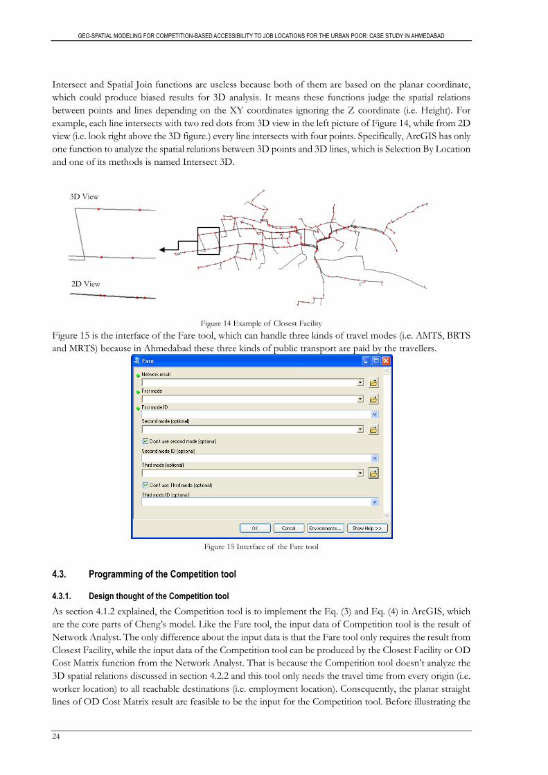
GEO-SPATIAL MODELING FOR COMPETITION-BASED ACCESSIBILITY TO JOB LOCATIONS FOR THE URBAN POOR: CASE STUDY IN AHMEDABAD
24
Intersect and Spatial Join functions are useless because both of them are based on the planar coordinate,
which could produce biased results for 3D analysis. It means these functions judge the spatial relations
between points and lines depending on the XY coordinates ignoring the Z coordinate (i.e. Height). For
example, each line intersects with two red dots from 3D view in the left picture of Figure 14, while from 2D
view (i.e. look right above the 3D figure.) every line intersects with four points. Specifically, ArcGIS has only
one function to analyze the spatial relations between 3D points and 3D lines, which is Selection By Location
and one of its methods is named Intersect 3D.
Figure 14 Example of Closest Facility
Figure 15 is the interface of the Fare tool, which can handle three kinds of travel modes (i.e. AMTS, BRTS
and MRTS) because in Ahmedabad these three kinds of public transport are paid by the travellers.
Figure 15 Interface of the Fare tool
4.3. Programming of the Competition tool
4.3.1. Design thought of the Competition tool
As section 4.1.2 explained, the Competition tool is to implement the Eq. (3) and Eq. (4) in ArcGIS, which
are the core parts of Cheng’s model. Like the Fare tool, the input data of Competition tool is the result of
Network Analyst. The only difference about the input data is that the Fare tool only requires the result from
Closest Facility, while the input data of the Competition tool can be produced by the Closest Facility or OD
Cost Matrix function from the Network Analyst. That is because the Competition tool doesn’t analyze the
3D spatial relations discussed in section 4.2.2 and this tool only needs the travel time from every origin (i.e.
worker location) to all reachable destinations (i.e. employment location). Consequently, the planar straight
lines of OD Cost Matrix result are feasible to be the input for the Competition tool. Before illustrating the
3D View
2D View

GEO-SPATIAL MODELING FOR COMPETITION-BASED ACCESSIBILITY TO JOB LOCATIONS FOR THE URBAN POOR: CASE STUDY IN AHMEDABAD
25
implementation processes, it is better to show the example of Figure 16, which could make the following
explanations clear.
In Figure 16, every employment location has different kinds of jobs. The lines of Figure 16 are the shortest
route from every worker location to reachable job locations. These shortest routes can be produced by the
Network Analyst of ArcGIS (Closest Facility or OD Cost Matrix). The attribute table of these shortest
routes is Table 2 for the example in Figure 16. In this attribute table, The Name field means each worker
location goes to which employment location. So the left words of hyphen are the labels of worker locations
and the right side of words are the labels of employment locations. The Time field of Table 2 is the travel
time of every route. Subsequently, it is the descriptions about implementation of Eq. (3) and Eq. (4). The
first phase is to implement Eq. (3) and the second phase is to implement Eq. (4).
Figure 16 Example of competition model
Table 2 Results of Network Analyst
1. First phase
For the implementation of Eq. (3), the key point is to know which employment locations compete for one
worker location. And then, according to the Eq. (3), we can find which job location is better or more
attractive for this worker location. For example, employers of JA (i.e. 100 jobs) and JB (i.e. 40 jobs) compete
for workers of W2. If the results of diversity of jobs (i.e. Eq. (1)) and decay function (i.e. Eq. (2)) are
considered as 1, the competition factor of JA and JB is 5/7 and 2/7 respectively. As the section 2.2 explained,
the competition factor can also be treated as the attractiveness of a job location.
2. Second phase
The results of the first phase (i.e. Eq. (3)) are the input for the implementation of Eq. (4), which is divided
into three steps. Table 3 is the results of the Competition tool for Figure 16. The following illustrations are
based on Table 3.
1) First, it is to calculate how many workers of each worker location are attracted by every employment
location, which is the part of the numerator of Eq. (4) (i.e. Pji x Wi x f(tij)). Specifically, the number of
workers (i.e. Wi) multiplies the corresponding result of Eq. (3) (i.e. Pji) and decay function (i.e. Eq. (2)).
If we still use the above example in which the result of decay function is 1, the job location JA and JB
𝐽𝑗 : 𝑒𝑚𝑜𝑝𝑙𝑦𝑚𝑒𝑛𝑡/𝑗𝑜𝑏 𝑙𝑜𝑐𝑎𝑡𝑖𝑜𝑛 𝑗 (𝑗 = 𝐴, 𝐵, 𝐶)
𝑊𝑖 : 𝑤𝑜𝑟𝑘𝑒𝑟 𝑙𝑜𝑐𝑎𝑡𝑖𝑜𝑛 𝑖 (𝑖 = 1,2,3)
W1 15 workers
JA 100 jobs
Retail: 20
Bank: 10
Industry: 70
W2 25 workers JB 40 jobs Logistics: 25
Bank: 15
W3 30 workers JC 20 jobs Industry: 20
W2
W1
W3
JA
JB
JC

GEO-SPATIAL MODELING FOR COMPETITION-BASED ACCESSIBILITY TO JOB LOCATIONS FOR THE URBAN POOR: CASE STUDY IN AHMEDABAD
26
attract 17.857 (i.e. 25 x 5/7) workers and 7.143 workers (i.e. 25 x 2/7) from worker location W2
respectively.
2) The second step is to calculate the competition among workers. The key point is to know which worker
locations compete for one employment location. So we can calculate the total number of attracted
workers for each job location, which is the sum of first step based on the dominator of Eq. (4). Then,
the number of jobs of every employment location is divided by the corresponding sum. For instance,
workers of W2 and W3 look for jobs at location JA and JA actually attracts 17.857 workers from W2
and 18.75 workers from W3. The total number of attracted workers at JA is 36.607 (i.e. 17.857+18.75).
The competition among workers at JA is the number of jobs (i.e. 100) divided by the total number of
workers (i.e. 36.607). The result is the number of available jobs for every worker.
3) The third and last step of implementing Eq. (4) is to use the number of attracted workers of every
worker location (i.e. the result of the first step) multiplying the corresponding result of the second step.
Finally, summarize the total number of job opportunities for every worker location (see Table 4). In
Table 4, the FREQUENCE field is the number of reachable destinations for every worker location,
which only reflects the efficiency of physical infrastructure. And the SUM_Opport field is the final job
opportunities for each worker location computed by Cheng’s model.
Table 3 Job opportunities when diversity and decay factor are 1
Explanation of Table 3: WID is the labels of worker location and JID is the labels of job locations. Djobs and Dworkers are the discounted jobs and workers. The discounted jobs and workers are equal to the number of jobs and workers because the result of decay function is 1 in this example. Jcomp is the competition among jobs. Att_worker is the number of attracted workers and Wcomp is the competition among workers. Opport is the job opportunities for each worker location.
Table 4 Final job opportunities
In order to make the above explanation clearer, Table 5 is the relations between the fields of Table 3 and the
components of Cheng’s model. This table also shows every component of Cheng’s model is implemented in
which phase.
Field name Components of Cheng’s model Explanation and Phase
Djobs 𝐸𝑗𝐷𝑗 × 𝑓(𝑡
𝑘𝑗)
The number of discounted jobs
(First phase)
Jcomp 𝑃𝑗𝑘 =𝐸𝑗
𝐷𝑗 × 𝑓(𝑡𝑘𝑗 )
𝐸𝑠𝐷𝑠 × 𝑓(𝑡𝑘𝑠)𝑠
The competition among jobs/employers
(First phase)
Dworkers 𝑊𝑖 × 𝑓(𝑡𝑖𝑗 ) The number of discounted workers
(Second phase, first step)
Att_worker 𝑃𝑗𝑖 × 𝑊𝑖 × 𝑓(𝑡𝑖𝑗 ) The number of attracted workers
(Second phase, first step)
Wcomp 𝐸𝑗𝑗
𝑃𝑗𝑘 × 𝑊𝑘 × 𝑓(𝑡𝑘𝑗 )𝑘
The competition among workers
(Second phase, second step)

GEO-SPATIAL MODELING FOR COMPETITION-BASED ACCESSIBILITY TO JOB LOCATIONS FOR THE URBAN POOR: CASE STUDY IN AHMEDABAD
27
Opport 𝑄𝑖 = 𝐸𝑗 × 𝑃𝑗𝑖 × 𝑊𝑖 × 𝑓(𝑡𝑖𝑗 )𝑗
𝑃𝑗𝑘 × 𝑊𝑘 × 𝑓(𝑡𝑘𝑗 )𝑘
The final job opportunities
(Second phase, third step)
Table 5 Relations between the table fields and components of Cheng’s model
4.3.2. Functions used in ArcGIS for the Competition tool
Based on the design thought of the Competition tool, this section explains which functions of ArcGIS and
Python used for programming this tool. There are three aspects in this section, which are preparation, the
first phase and second phase of design thought.
1. Preparation
Before starting to implement two phases of design thought mentioned in section 4.3.1, it is necessary to
finish the preparation for the following implementation. Specifically, the preparation is to copy the related
data (i.e. the number of jobs, the number of workers and the diversity of jobs) from other feature classes to
the attribute table of Network Analyst. That is because the attribute table of Network Analyst has the
relation between worker locations and job locations (i.e. people from worker locations look for jobs in which
employment locations and employers from job locations look for workers in which worker locations). This
relation is the key point to calculate Cheng’s model. Therefore, this research chooses the attribute table of
Network Analyst as the base table and all related factors (e.g. the diversity of jobs, two-side competition etc)
and the final results are shown in this table like Table 3. For the preparation, the Field Calculator, Add Field
and Join field function are adopted. The Field Calculator function is used with Python to extract the labels of
worker and job locations. For example, the values of WID field of Table 3 are extracted from the Name field.
The Add Field function is to create new fields in the attribute table of Network Analyst like the WID field of
Table 3. The Join field function is to copy the number of jobs and workers into the attribute table such as the
jobs and workers field in Table 3.
2. The first phase of design thought
This phase is to calculate the competition among jobs by Python. The SearchCursor function from Arcpy
module of ArcGIS can transfer the number of jobs in Python. According to the first phase of section 4.3.1
explained, this phase should make sure the attribute table sorting by the labels of worker locations in order to
know which employment location look for workers from the same worker location. In Python, the list can
keep this order. Then, the result of competition among jobs is calculated in Python and this result is copies
into the attribute table by UpdateCursor function from Arcpy module. In Table 3, the Jcomp field is the
result of this phase.
3. The second phase of design thought
The second phase has three steps as section 4.3.1 shown. For the first step, the Field Calculator is used to
calculate the number of attracted workers (e.g. Att_worker field of Table 3). The second step is to compute
the competition among workers, which is similar to the calculation of competition among jobs because both
competitions need to be calculated in sequence. The data of this phase is necessary to sort by the labels of
job locations (see the second phase of section 4.3.1). The SearchCursor function copies the number of
workers in Python. And the list of Python keeps the required order. Then, the competition among workers
is calculated in Python and this result is also copied into the attribute table by UpdateCursor function (e.g.
Wcomp field of Table 3). The third step is computed by the Field Calculator and Statistics function of
ArcGIS. The number of jobs multiplying the corresponding competition among workers is done by the
Field Calculator. The Statistics function produces the final result like Table 4.

GEO-SPATIAL MODELING FOR COMPETITION-BASED ACCESSIBILITY TO JOB LOCATIONS FOR THE URBAN POOR: CASE STUDY IN AHMEDABAD
28
All of the above functions are encapsulated into one package, which is the Competition tool. Figure 17 is the
interface of this tool in ArcGIS
Figure 17 Interface of the Competition tool
4.4. Interpretation of the results
This section has three parts to explain how the components of Cheng’s model influences the final job
opportunities based on the example of Figure 16. The first part discusses the effect of the decay function.
The second part is about the effect of diversity factor, which was treated as an elastic factor in Cheng’s
model. And the third part is to explain how the competition factors influence the result of Cheng’s model.
Then, this research gives a brief explanation about how to use the results of Cheng’s model in urban
planning.
4.4.1. The effect of decay function in Cheng’s model
Cheng’s model distributes the existing opportunities to each worker location and doesn’t have some
opportunities remained. The decay function is one of the factors to influence the distribution of job
opportunities. Table 6 is the result of Cheng’s model when beta is 0.5 and the diversity factor is 1. Table 3
and Table 6 are the same example, while the only difference is beta value. The beta value of previous one
is 0 and the later one is 0.5. We can see that W2 and W3 location can get 48.78 and 51.22 jobs from JA
respectively in Table 3. Their sum is still equal to the number of jobs in JA (i.e. 100 jobs). For Table 6, W2
and W3 gets 97.21 jobs and 2.79 jobs from JA respectively. The sum is still equal to the number of jobs at
JA location. So the decay function can change the distribution of jobs in Cheng’s model.
Table 6 Job opportunities when diversity factor is 1 but the beta of decay function is 0.5
4.4.2. The effect of diversity factor in Cheng’s model
According to the equation (1) (i.e. diversity of jobs), if an employment location has one kind of jobs, the
number of this type jobs is equal to the total number of jobs at this location (i.e. 𝐸𝑙𝑗 = 𝐸𝑗 ). This diversity of
jobs (i.e. 𝐷𝑗 ) at this employment location is zero and 𝐸𝑗𝐷𝑗 (in Eq. (3)) is 1. In contrast, if another employment
location has many types of jobs but the number of every type of jobs is equal, the diversity of jobs (i.e. 𝐷𝑗 ) is

GEO-SPATIAL MODELING FOR COMPETITION-BASED ACCESSIBILITY TO JOB LOCATIONS FOR THE URBAN POOR: CASE STUDY IN AHMEDABAD
29
1 at this job location and 𝐸𝑗𝐷𝑗 is equal to 𝐸𝑗 . Cheng et al. (2012, pg.3) explained the diversity as an elastic
factor and “the elasticity is between one (each additional type of job will affect the probability that a worker
from 𝑖 will be attracted by 𝑗) and zero (no additional type of jobs will affect the probability of a worker from
𝑖 to be assigned to 𝑗).”
The diversity function is the elasticity, which only influences the distribution of jobs. For example, Table 7 is
the result with diversity factor, which is calculated from Eq. (1). W2 can get 53.63 jobs from location JA
and W3 has 46.37 jobs from the same job location. Their sum is still equal to the number of jobs at JA
location (i.e. 100).
Table 7 Job opportunities when diversity factor is not 1 but decay factor is 1.
4.4.3. The effect of competition factors
The section explains which factors determine the two-side competition and how the two-side competition
affects on the job opportunities. Actually, the competition factors are determined by the Network Analyst,
the number of workers, the number of jobs, diversity factor and decay function. The Network Analyst
impacts on the number of reachable employment locations for each worker location. But it doesn’t mean
that more reachable job locations could provide more job opportunities because of the competition factor
in Cheng’s model. If we still use the example of Figure 16 but the road network is improved for W1 and
W2. W1 can reach two more job locations (i.e. JA and JC) and W2 can reach one more job location (i.e.
JC). The improvement is only for W1 and W2 worker locations and other things of this example don’t
change (see Table 8 and the diversity and decay factors are 1). From the view of accessibility analysis
without competition, the job accessibility of W1 and W2 should increase because they can reach more job
locations, while the result of Cheng’s model shows that the job accessibility of W2 decreases from 58.42
(see Table 4) to 57.14 (see Table 9). And only the job accessibility of W1 increases from 20.24 (see Table 4)
to 34.29 (see Table 9) after improvement of the road network (Table 4 is the result based on the original
road and Table 9 is the result based on the improved road network).
W1 and W2 have the different variations after the road network improved due to a series of changes. First,
the improvement of road network enhances the mobility for workers and employers. So from Table 3 and
Table 8, we can see that the job competition factor (i.e. Jcomp field) of JA to W2 and JB to W2 decline (i.e.
from 0.714 to 0.625 and from 0.286 to 0.25) because there is one more worker location (i.e. JC) compete
for workers from W2 with JA and JB. In other word, the attractiveness of JA and JB decrease due to one
more employment location going to W2. Therefore, the number of attracted workers (i.e. Att_worker field)
from W2 by JA and JB also declines, which influences the competition among workers (i.e. Wcomp field)
according to Eq. (4). The values of Wcomp field are the average number of jobs for every worker location.
If the value of Wcompe is bigger, more job opportunities are offered for every worker. In Table 3, JA and
JB can provide 2.732 and 1.349 jobs for every worker who lives in W2. However, in Table 8, both of JA
and JB can provide 2.286 jobs for every worker at location W2. This value could increase or decrease after
improvement the road network. Actually, this value (i.e. the competition among workers is shown in
Wcomp field) is affected by all the related worker locations and job locations. That is because Wcomp is
calculated from the number of attracted workers (i.e. Att_worker field), which is determined by the
number of workers and competition among jobs (i.e. Jcomp).
In a word, the JA and JB provide a fewer of jobs for W2 comparing to the result of original road network,
although JC can provide new jobs for W2 but the number of new jobs is less than the decreased number
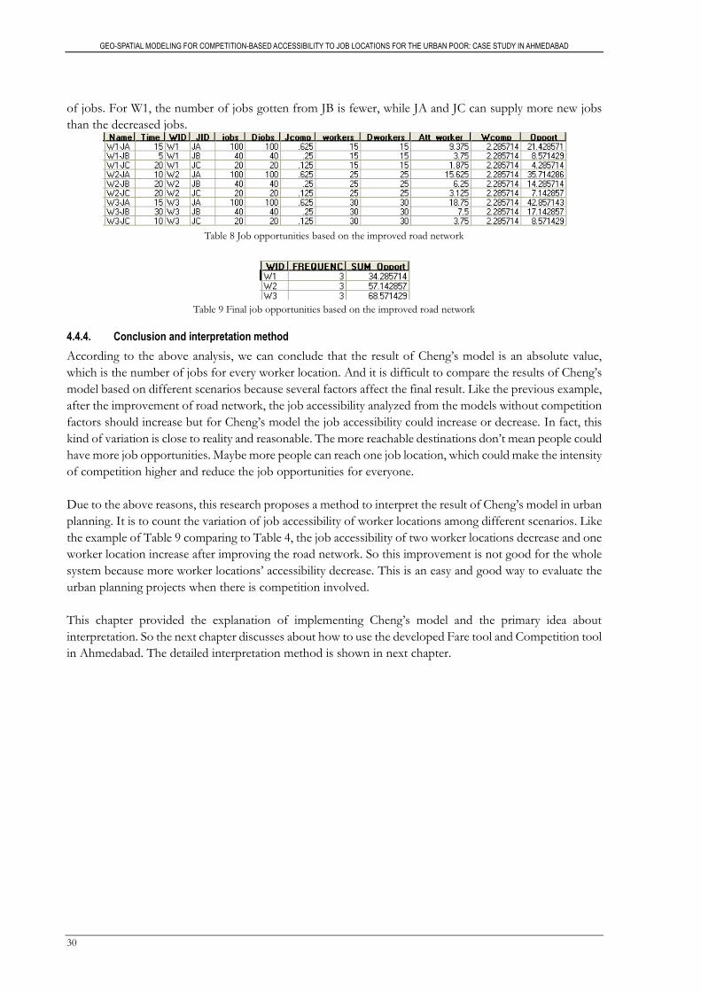
GEO-SPATIAL MODELING FOR COMPETITION-BASED ACCESSIBILITY TO JOB LOCATIONS FOR THE URBAN POOR: CASE STUDY IN AHMEDABAD
30
of jobs. For W1, the number of jobs gotten from JB is fewer, while JA and JC can supply more new jobs
than the decreased jobs.
Table 8 Job opportunities based on the improved road network
Table 9 Final job opportunities based on the improved road network
4.4.4. Conclusion and interpretation method
According to the above analysis, we can conclude that the result of Cheng’s model is an absolute value,
which is the number of jobs for every worker location. And it is difficult to compare the results of Cheng’s
model based on different scenarios because several factors affect the final result. Like the previous example,
after the improvement of road network, the job accessibility analyzed from the models without competition
factors should increase but for Cheng’s model the job accessibility could increase or decrease. In fact, this
kind of variation is close to reality and reasonable. The more reachable destinations don’t mean people could
have more job opportunities. Maybe more people can reach one job location, which could make the intensity
of competition higher and reduce the job opportunities for everyone.
Due to the above reasons, this research proposes a method to interpret the result of Cheng’s model in urban
planning. It is to count the variation of job accessibility of worker locations among different scenarios. Like
the example of Table 9 comparing to Table 4, the job accessibility of two worker locations decrease and one
worker location increase after improving the road network. So this improvement is not good for the whole
system because more worker locations’ accessibility decrease. This is an easy and good way to evaluate the
urban planning projects when there is competition involved.
This chapter provided the explanation of implementing Cheng’s model and the primary idea about
interpretation. So the next chapter discusses about how to use the developed Fare tool and Competition tool
in Ahmedabad. The detailed interpretation method is shown in next chapter.

GEO-SPATIAL MODELING FOR COMPETITION-BASED ACCESSIBILITY TO JOB LOCATIONS FOR THE URBAN POOR: CASE STUDY IN AHMEDABAD
31
5. ACCESSIBILITY ANALYSIS AND RESULTS
In this chapter, the competition-based accessibility measure for Ahmedabad (i.e. Cheng’s model) is
demonstrated. First, we discuss the data preparation, which is about how to aggregate data, calculate the beta
parameter of decay function and other related descriptions. The second section provides the scenarios in
this research. The third section explains how to interpret the result of Cheng’s. The fourth section shows
some discussions about which factors influence job accessibility of the urban poor in Ahmedabad according
to the interpretation.
5.1. Data preparation
5.1.1. Locations of employment and potential workers
The base data of employment and slum locations is 100 x 100m grid cells, which is collected by AMC and
CEPT University. Each cell is one job or slum location and the centroid of a cell represents the specific
origin or destination. The spatial units are the key point to influence the accuracy of accessibility measure
(Apparicio et al., 2008). And the unit size also determines the feasibility of calculation in a computer. Like the
base data, there are 12078 job locations and 1752 worker locations. With such amount of data it is difficult to
work out results by the computer because of around 12 million OD lines and let alone the 3D routes of
Closest Facility analysis. In order to reduce the burden for computation and keep acceptable accuracy, this
research aggregates the 100 x 100m cell into 500 x 500m for slum locations (i.e. the right side of Figure 18).
For the employment locations, the spatial unit is aggregated into 1000 x 1000m (i.e. the left side of Figure 18).
In reality, the distribution of employment locations is always concentrated in one place. For example, Cheng
et al. (2012) chose only 45 major employment locations to analyze the competition-based job accessibility
(i.e. Cheng’s model) in Amsterdam. Consequently, this research makes the spatial unit of employment larger,
while there are still 255 job locations, which has the relative high accuracy compare to (Cheng et al., 2012).
Figure 18 Aggregated number of jobs and workers
The base data has four types of slum or Chawl. And depending on the quality of houses (see Section 3.2) the
urban poor is classified into three classes as Table 10 shows. Based on the suggestions from Talat Munshi2
and (Ray, 2010), six kinds of job sectors are reclassified into three categories and every category of jobs
corresponds to a certain level of poverty people (Table 10). Specifically, all kinds of job locations are 255.
2 An associate Professor in CEPT University

GEO-SPATIAL MODELING FOR COMPETITION-BASED ACCESSIBILITY TO JOB LOCATIONS FOR THE URBAN POOR: CASE STUDY IN AHMEDABAD
32
Either the very poor or middle poor people, there are 251 employment locations for them and 255
employment locations for the least poor. The number of worst quality of houses (i.e. Huts & Kutccha) is
351 and the worse houses (i.e. Semi-pucca) are 318 as well as the bad houses are 261. Then, this number
of potential workers estimation is from the World Bank project (Zuidgeest et al., 2012), which assumes
there are 2 potential workers in every kind of house. This research also has the data about 21 SEWSH (see
Section 3.2) locations where people living can find all kinds of jobs.
House type Poverty degree Job type
Huts & Kutccha Very poor Transport & Storage, Small-scale industry
Semi-pucca Middle poor Retail, Medium-scale industry
Pucca Least poor Government sector, education jobs, jobs in hotels & boarding, office & commercial jobs, Large-scale industry
Table 10 Relationship between house and job type
5.1.2. Decay function and diversity factor
1) Time decay function
The time decay function is taken from the World Bank project. The report from that project mentions
that when travel time is 30 minutes from worker location to employment location, 31% of workers are
willing to go there, represented by taking 0.03838 as the beta parameter in the negative exponential
function (Figure 19).
Figure 19 Time decay function
2) Fare decay function
For fare decay function, it is also the negative exponential function. As (Mahadevia et al., 2012) found, poor
people in Ahmedabad wanted to spend less than 5 per cent of their total household expenditure on transport
and 65% of households preferred not to spend anything on transport. Thus, this beta parameter is 0.52491
because only 35% of poor people could take public transport for travelling (Figure 20).

GEO-SPATIAL MODELING FOR COMPETITION-BASED ACCESSIBILITY TO JOB LOCATIONS FOR THE URBAN POOR: CASE STUDY IN AHMEDABAD
33
Figure 20 Fare decay function
The detailed fare structure of AMTS is in section 4.2.1. For BRTS and MRTS, both of them are under
construction in Ahmedabad. According to the BRTS report (Ahmedabad Municipal Corporation et al.,
2008), the fare of BRTS will be increased by 125% based on the fare of AMTS. Since Bus Rapid Transit is
often regarded as the on-the-road metro because the character of BRT is very similar to the metro.
Therefore, this research assumes that the MRTS has the same fare structure as that of BRTS in Ahmedabad.
3) Diversity factors
The diversity factors are 1 and there are two reasons. First, any scenario has the same number of job types
for each employment location. So the diversity factor could have a little impact on the final results. And this
research considers that the diversity of jobs is not an important factor to attract the workers, while the
number of jobs is the key to attract poor people. Second, even though the diversity factor is treated as the
elasticity for the attractiveness of a job location, the diversity is calculated by Eq. (1) derived from the
entropy, which are not like factors like competition, decay function having the social meanings.
5.1.3. Road network
As section 3.4.2 shown, the road network of this research is 3D. And there are five travel modes in this
network, which are walking, cycling, bus (AMTS), Bus Rapid Transit (BRTS) and metro (MRTS). Figure 21
is the current and under constucted public transport systems in Ahmedabad. This figure is made by the 2D
view in order to show the network of every public transport clearly. The AMTS has a very developed
network comparing to the BRTS and MRTS. Table 11, which is also from the World Bank project, is the
related properties of every travel mode. The Access means that people spend how much time on waiting for
a public transport and the Egress is the get-off time. The access and egress time are the impedance of links
between two different travel modes.
Mode Speed (km/h) Access (min) Egress (min)
Walking 3.5 N/A N/A
Cycling 12 N/A N/A
AMTS 15 - 20 10 1
BRTS 25 5 2
MRTS 35 3.75 2
Table 11 Properties of road network

GEO-SPATIAL MODELING FOR COMPETITION-BASED ACCESSIBILITY TO JOB LOCATIONS FOR THE URBAN POOR: CASE STUDY IN AHMEDABAD
34
Figure 21 Public transport systems in Ahmedabad
5.1.4. Travel time threshold
There are two reasons for defining a travel time threshold. First, according to the decay function of Cheng’s
model, if the travel time is too large, the effect will be less, which affects the final results little. So it is not
necessary to analyze those locations, which are too far away from the worker location. Second, Bhatt (2003)
found the urban poor in Ahmedabad cycling10-12 km every day go to work. In other words, the poor people
could travel around 60 minutes for commuting daily. Consequently, this research defines a travel time
threshold for the urban poor, which is reasonable and good to increase the efficiency of calculation.
The travel time threshold is 60 minutes. But the time threshold of Network Analyst should be less than 60
minutes because of the intra-zone problem. Figure 22 shows the intra-zone problem in this research. In the
Network Analyst, it is assumed that all of people living in the square cell have the same results as people in
the centroid. In order to measure the accessibility objectively, the average intra-zone travel distance (i.e.
Maximum intra-zone distance/2) and walking speed are used to compute the intra-zone travel time. This
time is 20 minutes, including the travelling time in slum cell and employment cell. So the travel time
threshold for Network Analyst is 40 minutes.
Figure 22 Intra-zone problem
Distance between centroids
Maximum intra-zone distance
Centroid of a cell
40 min 500 meters 1000 meters
Slums
Jobs

GEO-SPATIAL MODELING FOR COMPETITION-BASED ACCESSIBILITY TO JOB LOCATIONS FOR THE URBAN POOR: CASE STUDY IN AHMEDABAD
35
5.1.5. Dwelling places change from Slums/Chawls to SEWSH
As section 3.2 mentioned, the government of Ahmedabad builds the SEWSH, which has better living
environment and conditions. The 21 SEWSH locations are the new houses for the urban poor. Some poor
people could change their living places from Slums/Chawls to SEWSH. However, if the job accessibility
analysis is only for the 21 SEWSH locations, it must be biased from the reality using Cheng’s model. That is
because the poor people living in SEWSH don’t only compete for jobs with themselves, they but also
compete with the people who still live in Slums/Chawls. Therefore, if we want to measure the job
accessibility of SEWSH, it is necessary to know which Slums/Chawls’ poor people change their dwelling
places to SEWSH. This research assumes that the dwelling changes for the poor people from Slums/Chawls
to SEWSH depend on the Euclidean distance and the nearest Slums/Chawls to one SEWSH location has
the highest priority. Due to the limited capacity of SEWSH, some poor people from Slums/Chawls will
change their dwelling places as SEWSH but there are still remained poor people who still live in
Slums/Chawls. Based on this assumption, the job accessibility analysis of SEWSH can reflect the effect of
this housing project.
Figure 23 shows the results of dwelling changes. Compare to Figure 8, some Slums/Chawls locations nearby
SEWSH locations disappear in Figure 23 (i.e. the hollow points) because all of the urban poor from these
Slums/Chawls locations move to live in SEWSH. The poor people of some locations are divided into two
parts. Some of them move to live in SEWSH and the remained people are still living in Slums/Chawls
because of the limited capacity of SEWSH. Finally, the 353 worker locations and 21 SEWSH locations are
merged together as 357 worker locations. The workers from 35 Slum/Chawl locations move to live in
SEWSH locations. There are 17 Slums/Chawls disappeared after rearranging the worker locations. All of
workers from the 17 locations move to live in SEWSH.
Figure 23 Slums/Chawls and SEWSH locations after changing dwelling places

GEO-SPATIAL MODELING FOR COMPETITION-BASED ACCESSIBILITY TO JOB LOCATIONS FOR THE URBAN POOR: CASE STUDY IN AHMEDABAD
36
5.2. Explanation about research scenarios
One of the research goals is to figure out the job accessibility of the urban poor in Ahmedabad and evaluate
the effect of AMTS, BRTS, MRTS and SEWSH projects. This research defines the following the scenarios
matrix (i.e. Table 12). For the combinations of travel modes, there are four options in this matrix and each
combination has five kinds of workers to analyze according to the worker classification in section 5.1.1 and
the dwelling changes described in section 5.1.5. The time and fare decay functions are also involved in the
scenarios of three combinations of travel modes (i.e. except only walking).
Combination of travel modes
Worker classification Decay function
Walking
Very poor
Only time decay function used
Middle poor
Least poor
All poor3
Slums/Chawls to SEWSH4
Walking
AMTS
Very poor
Time and fare decay function used
Middle poor
Least poor
All poor
Slums/Chawls to SEWSH
Walking
AMTS
BRTS
Very poor
Time and fare decay function used
Middle poor
Least poor
All poor
Slums/Chawls to SEWSH
Walking
AMTS
BRTS
MRTS
Very poor
Time and fare decay function used
Middle poor
Least poor
All poor
Slums/Chawls to SEWSH
Table 12 Research scenario matrix
According to this scenario matrix and previous data preparation, the following explanations are about the
job accessibility and evaluation of the relevant projects.
5.3. Explanation about the Interpretation
This section has two parts. First, one specific example is chosen to do the detailed analysis, which can figure
out how Cheng’s model measures the job accessibility for the urban poor in Ahmedabad. Second, based on
the first example, a method is proposed to interpret the result of Cheng’s model. Before analyzing the
results, some abbreviations are explained in Table 13.
Abbreviation Explanation
W Only walking
WA Walking and AMTS used
WAB Walking, AMTS, BRTS used
WABM Walking, AMTS, BRTS and MRTS used
Table 13 Explanation about abbreviations
3 All poor: All worker locations except SEWSH without changing the dwelling places 4 Slums/Chawls to SEWSH: All worker locations after changing the dwelling places include SEWSH

GEO-SPATIAL MODELING FOR COMPETITION-BASED ACCESSIBILITY TO JOB LOCATIONS FOR THE URBAN POOR: CASE STUDY IN AHMEDABAD
37
5.3.1. Specific example exploration
This section analyzed the job accessibility for all worker locations (i.e. only Slums/Chawls except SEWSH)
to all job locations when the combination of travel modes changes from W to WA. In order to formulate
the interpretation method, this research selects one specific worker location from the result. This example
is about worker location 1421, which job accessibility grows a lot from W to WA (i.e. from 1366 to 33928).
Table 14 is the result by only walking. The workers from 1421 can reach 4 job locations, which are 369,
331, 368 and330. And only workers from 1421 go to these four job locations. Thus, the values of Opport
are equal to that of All_job field because no one from other worker locations competes with workers from
1421 for jobs at these four job locations. And the final job opportunities are the sum of Opport field,
which is 1366.
Table 14 Results of worker location 1421 by walking
After using walking and AMTS together (i.e. WA), workers from 1421 can reach 8 job locations as Table 15
shown. Besides the previous four job locations, workers of this location can get new jobs from other
employment locations (i.e. 444, 481, 443 and 555), which is the main contribution for job accessibility
increasing.
Table 15 Results of worker location 1421 by walking and AMTS
For the previous four job locations (i.e. 369, 331, 368 and330), only job location 369 attracts another three
worker locations as Table 16 shows, which are 2097, 2172 and 2247. So some jobs from 369 are distributed
to other worker locations by WA, while these jobs originally belong to worker location 1421 by walking (i.e.
W). The workers from 1421 get fewer jobs from 369 when the combination of travel modes changes from W
to WA. But workers from 1421 can get much more jobs from other job locations by WA.
Specifically, the number of job opportunities for 1421 worker location is determined by the number of
attracted workers and the competition among workers according to Eq. (4) (The specific explanation is the
third step of second phase in section 4.3.1). It is interesting that the competition among workers (i.e. Wcomp
field) in job location 369 doesn’t cause the job accessibility decreasing for 1421 worker location because the
Wcomp by W is 0.93 and Wcomp by WA is 13.90. So this increase from 0.93 to 13.90 means more jobs for
every worker at location 1421 and it can’t cause the decrease of job accessibility. The main reason to cause
the job opportunities decreasing for 1421 location is the number of attracted workers (i.e. Att_worker field)
at job location 369 declining from 315.65 (see Table 14) to 15.75 (see Table 15). It means that fewer workers
want to find jobs at job location 369, which results from the attractiveness of 369 (i.e. Jcomp
field/competition among jobs) decreasing from 0.309 (see Table 14) to 0.015 (see Table 15). So the 369
employment location offering fewer jobs for worker location 1421 is caused by the two-side competition
and the two-side competition is determined by the Network Analyst, which influences how many worker
locations compete for one job location and vice versa.
Table 16 Results of job location 369 by walking and AMTS

GEO-SPATIAL MODELING FOR COMPETITION-BASED ACCESSIBILITY TO JOB LOCATIONS FOR THE URBAN POOR: CASE STUDY IN AHMEDABAD
38
Through this detailed analysis, we can see it is very complex to interpret the result for every worker
location. The result interpretation, therefore, should be from the overall view for all worker locations like
section 4.4.4 concluded. In 353 worker locations, 214 locations can get more jobs and other 139 locations
lose some opportunities from W to WA. The AMTS can improve 60.6% of worker locations’ job
accessibility. For the improved worker locations (i.e. 214 locations), they can get 233562 more jobs by WA.
The number of their job opportunities increases 43.4% by WA comparing to the number of their jobs by
W (i.e. 537681).
5.3.2. Interpretation method
Based on the previous section analysis and the conclusion from section 4.4.4, this research formulates the
following equations for interpretation: 𝑉 = 𝐴𝑖,𝑗 ,𝑘 − 𝐴𝑖 ′ ,𝑗 ′ ,𝑘 ′ (10)
𝑃𝑣 = V/𝐴𝑖 ′ ,𝑗 ′ ,𝑘 ′ (11)
𝑃𝐼 = 𝑛𝑖 ,𝑗 ,𝑘−𝑖 ′ ,𝑗 ′ ,𝑘 ′ /𝑁𝑖 ′ ,𝑗 ′ ,𝑘 ′ (12)
Eq. (10): 𝑉 is the accessibility difference of every worker location between two different scenarios, 𝐴 is
the number of job opportunities of every worker location from different scenarios, 𝑖 and 𝑖′ are the five
kinds of worker locations (i.e. Worker classification of Table 12), 𝑗 and 𝑗′ are the four combinations of
travel modes (i.e. Combination of travel modes in Table 12), 𝑘 and 𝑘′ are two different decay functions (i.e.
Decay function of Table 12). So 𝑖, 𝑗, 𝑘, 𝑖′ , 𝑗′ , 𝑘 ′ indicate which scenario is analyzed.
Eq. (11): 𝑃𝑣 is the percent of variation of job accessibility for every worker location between two
different scenarios. The other variables are the same as Eq. (10)
Eq. (12): 𝑃𝐼 is the percent of improvement of job accessibility for all analyzed worker locations, 𝑛 is the
number of positive 𝑉 or 𝑃𝑣, 𝑁 is the total number of analyzed worker locations, 𝑖, 𝑗, 𝑘 − 𝑖′ , 𝑗′ ,𝑘′ is the
label of comparison between which two scenarios, 𝑖, 𝑗, 𝑘, 𝑖′ , 𝑗′ , 𝑘 ′ are the same as Eq. (10)
If the result of equation (10) or (11) is positive for one worker location, the job accessibility of second
scenario (i.e.𝐴𝑖 ,𝑗 ,𝑘 ) is higher than the job accessibility of first scenario (i.e. 𝐴𝑖 ′ ,𝑗 ′ ,𝑘 ′ ) and vice visa. The
number of positive value 𝑉 or 𝑃𝑣 is more, the better of second scenario is. The core ideas about job accessibility analysis in Ahmedabad are the above explanations.
5.4. Accessibility results
Although there are lots of results produced based on the scenarios (i.e. Table 12), this research chooses
the important and useful results discussed in this section, which is divided into four parts. The first part is
about the job accessibility of all workers and jobs, which finds out the effect of different public transport
modes on all poor people. The second part is about the job accessibility for three classes of poor people.
The third part is about the effect of SEWSH. It is to analyze the job accessibility if the poor people change
their dwelling places as section 5.1.5 shown.
5.4.1. Job accessibility of all worker locations
This section has two parts, which are about the job accessibility of all worker locations. The first part is to
compare the job accessibility among different transport scenarios and find the best combination of travel
modes to improve the job accessibility for the urban poor. The second part is to compare the differences
between fare and time decay function for the job accessibility of all the worker locations.
1) The best travel mode for improving job accessibility
In order to find the most efficient travel mode for improving accessibility, this section compares three
combinations of travel modes with two different decay functions. Figure 24 is the job accessibility from

GEO-SPATIAL MODELING FOR COMPETITION-BASED ACCESSIBILITY TO JOB LOCATIONS FOR THE URBAN POOR: CASE STUDY IN AHMEDABAD
39
Cheng’s model when the time decay function is used. The left top map is the results by W5 and the right
top map is the results by WA. The biggest map is about the comparison between the above two maps.
Specifically, the comparison formula is from Eq. (10) and Eq. (11):
𝑃𝑣 = (𝐴𝐴𝑙𝑙 𝑝𝑜𝑜𝑟 ,𝑊𝐴 ,𝑇𝑖𝑚𝑒 𝑑𝑒𝑐𝑎𝑦 − 𝐴𝐴𝑙𝑙 𝑝𝑜𝑜𝑟 ,𝑊 ,𝑇𝑖𝑚𝑒 𝑑𝑒𝑐𝑎𝑦 )/𝐴𝐴𝑙𝑙 𝑝𝑜𝑜𝑟 ,𝑊 ,𝑇𝑖𝑚𝑒 𝑑𝑒𝑐𝑎𝑦 (13)
The biggest map shows the accessibility of some worker locations decrease, while other locations increase
from W to WA. We can’t judge whether the WA is better than W by the map. Consequently, according to
the interpretation method from section 5.3.2, this research makes Table 17, which is the Percent of
improvement from Eq. (12). And there are three scenarios in this table, which are changing the
combination of travel modes from W to WA (only using time decay function), and from WA to WABM
(using time decay and fare decay function separately). The combination of travel modes changes from W
to WA or from WA to WABM, the Percent of improvement of three scenarios is around 60% and there is
a little difference. So we can’t find which combination of travel modes is the best for improving job
accessibility. But most of worker locations can get more job opportunities when the AMTS, BRTS and
MRTS are provided.
Scenarios Percent of improvement (PI)
W-WA (time decay) 60.6%
WA-WABM (time decay) 59.5%
WA-WABM (fare decay) 61.3%
Table 17 Comparison among W, WA and WABM for all worker locations
Explanation of Table 17 and Table 18:
W-WA: the scenario changes from W to WA, which is the effect of AMTS. W is the first scenario and WA is the second one.
WA-WANM: the scenario changes from WA to WABM, which measures the effect of BRTS and MRTS. WA is the first scenario and WABM is the second one.
In the following sections, W-WA and WA-WABM has the same meaning as them in Table 17
In order to find the most efficient combination of travel modes, Table 18 shows the total number of jobs
increase for the worker locations where job accessibility improved. It is evident that no matter which kind of
decay function, the AMTS is most efficient public transport and it can make the jobs increase 43.4%
comparing to the number of jobs accessed by only walking (i.e. W). For BRTS and MRTS, although both
travel modes can improve the job accessibility, the effect is not good as that of AMTS. That is because the
number of jobs only increases around 3.5% when the combination of travel modes changes from WA to
WABM.
Total number of increased job opportunities Increased percent
W-WA (time decay) 233562 43.4%
WA-WABM (time decay) 21044 3.5%
WA-WABM (fare decay) 24138 3.6%
Table 18 Number of increased job opportunities between different combinations of travel modes
5 W, WA, WAB and WABM are explained in Table 13 at the beginning of section 5.3

GEO-SPATIAL MODELING FOR COMPETITION-BASED ACCESSIBILITY TO JOB LOCATIONS FOR THE URBAN POOR: CASE STUDY IN AHMEDABAD
40
Figure 24 Comparison job opportunities of only walking with that of walking and AMTS6
6 Variation is defined as the equation (13) in section 5.4.1

GEO-SPATIAL MODELING FOR COMPETITION-BASED ACCESSIBILITY TO JOB LOCATIONS FOR THE URBAN POOR: CASE STUDY IN AHMEDABAD
41
2) The effect of time and fare decay function
The top two maps of Figure 25 are the job opportunities with time and fare decay function using all travel
modes (i.e. WABM). The biggest picture is the difference between the top two maps and it is also
calculated by the equation (10) and (11).
𝑃𝑣 = (𝐴𝐴𝑙𝑙 𝑝𝑜𝑜𝑟 ,𝑊𝐴𝐵𝑀 ,𝐹𝑎𝑟𝑒 𝑑𝑒𝑐𝑎𝑦 − 𝐴𝐴𝑙𝑙 𝑝𝑜𝑜𝑟 ,𝑊𝐴𝐵𝑀 ,𝑇𝑖𝑚𝑒 𝑑𝑒𝑐𝑎𝑦 )/𝐴𝐴𝑙𝑙 𝑝𝑜𝑜𝑟 ,𝑊𝐴𝐵𝑀 ,𝑇𝑖𝑚𝑒 𝑑𝑒𝑐𝑎𝑦 (14)
Like previous section shown, we can’t evaluate the effect of two decay functions only through Figure 25.
So we use the equation (12) (i.e. 𝑃𝐼). There two kinds of combinations of travel modes (i.e. WA and
WABM) generating the fare. So the comparisons have two formulas:
𝑃𝐼𝑊𝐴 = 𝑛𝐴𝑙𝑙 𝑝𝑜𝑜𝑟 ,𝑊𝐴 ,𝐹𝑎𝑟𝑒 𝑑𝑒𝑐𝑎𝑦 −𝐴𝑙𝑙 𝑝𝑜𝑜𝑟 ,𝑊𝐴 ,𝑇𝑖𝑚𝑒 𝑑𝑒𝑐𝑎𝑦 /𝑁𝐴𝑙𝑙 𝑝𝑜𝑜𝑟 ,𝑊𝐴 ,𝑇𝑖𝑚𝑒 𝑑𝑒𝑐𝑎𝑦 (15)
𝑃𝐼𝑊𝐴𝐵𝑀 = 𝑛𝐴𝑙𝑙 𝑝𝑜𝑜𝑟 ,𝑊𝐴𝐵𝑀 ,𝐹𝑎𝑟𝑒 𝑑𝑒𝑐𝑎𝑦 −𝐴𝑙𝑙 𝑝𝑜𝑜𝑟 ,𝑊𝐴𝐵𝑀 ,𝑇𝑖𝑚𝑒 𝑑𝑒𝑐𝑎𝑦 /𝑁𝐴𝑙𝑙 𝑝𝑜𝑜𝑟 ,𝑊𝐴𝐵𝑀 ,𝑇𝑖𝑚𝑒 𝑑𝑒𝑐𝑎𝑦 (16)
The Percent of improvement values of these two scenarios (i.e. 𝑃𝐼𝑊𝐴 and 𝑃𝐼𝑊𝐴𝐵𝑀 ) are around 43.0%. It
means around 43.0% of worker locations can get more jobs when change the time decay function as fare
decay function. So 57% of worker locations lose some job opportunities because the time and fare decay
function have different effects for distributing jobs. And we can conclude that more than 50% of worker
locations are sensitive to the fare.

GEO-SPATIAL MODELING FOR COMPETITION-BASED ACCESSIBILITY TO JOB LOCATIONS FOR THE URBAN POOR: CASE STUDY IN AHMEDABAD
42
Figure 25 Comparison job opportunities of time decay with that of fare decay by all travel modes7
7 Variation is defined as the equation (14) in section 5.4.1.

GEO-SPATIAL MODELING FOR COMPETITION-BASED ACCESSIBILITY TO JOB LOCATIONS FOR THE URBAN POOR: CASE STUDY IN AHMEDABAD
43
5.4.2. Job accessibility of three levels of poor people
The following explanation chooses the average number of reachable job locations and job opportunities
to analyze accessibility in Ahmedabad. It can show which class of poor people has more jobs.
From the left side of Figure 26, we can see that if there is one more travel mode, the number of reachable
employment locations increases. The significant increment is between W and WA, while there is a little
increment among WA, WAB and WABM. For one certain combination of travel modes, the number of
reachable job locations has tiny variations among three levels of poor people.
Let’s explore the detailed information from the right side of Figure 26. The average number of job
opportunities grows obviously between W and WA. From WA to WAB, the increment is a little, while there
is no significant variation between WAB and WABM. For the three different categories of poor people in
one combination of travel modes, the very poor people has the least job chances and the other two kinds of
people (i.e. the middle poor and least poor) can get much more opportunities. Moreover, the least poor
people have more jobs than that of the middle poor people.
Figure 26 Average job opportunities for three levels of poor people
The above analysis is somehow like the cumulative analysis and there are two reasons. First, the number of
reachable job locations doesn’t include the competition and decay factor. Second, the average number of job
opportunities for every worker location doesn’t reflect the competition and decay factor. That is because the
competition and decay factor can be reflected by the job accessibility of every single worker location so the
sum of jobs is like the cumulative measure. The average number of job opportunities is from the sum of all
the jobs divided by the number of worker locations. So the above analysis is like cumulative measure, which
is to show the difference about the number of jobs among three classes of poor people.
And then the following sections discuss the job accessibility of three levels of poor people with competition
and decay factor. The key point is also to use the interpretation method in section 5.3.2. The first part is the
comparison among W, WA and WABM using time decay function. The second part is about the effect of
fare decay function for three levels of poor people and the comparison between time and fare decay function
for the three classes of poor people
1) The effect of different travel modes with time decay function
Figure 27 is the job accessibility variation between different combinations of travel modes. This figure
shows the Percent of improvement for three levels of poor people by different combinations of travel
modes with time decay function. Table 19 is the specific explanation about Figure 27.

GEO-SPATIAL MODELING FOR COMPETITION-BASED ACCESSIBILITY TO JOB LOCATIONS FOR THE URBAN POOR: CASE STUDY IN AHMEDABAD
44
Scenarios Bar color in Figure 27
Equations
W-WA
Blue bar 𝑃𝐼𝑏𝑙𝑢𝑒 = 𝑛𝑉𝑒𝑟𝑦 𝑝𝑜𝑜𝑟 ,𝑊𝐴 ,𝑇𝑖𝑚𝑒 𝑑𝑒𝑐𝑎𝑦 −𝑉𝑒𝑟𝑦 𝑝𝑜𝑜𝑟 ,𝑊 ,𝑇𝑖𝑚𝑒 𝑑𝑒𝑐𝑎𝑦 /𝑁𝑉𝑒𝑟𝑦 𝑝𝑜𝑜𝑟 ,𝑊,𝑇𝑖𝑚𝑒 𝑑𝑒𝑐𝑎𝑦
Red bar 𝑃𝐼𝑟𝑒𝑑 = 𝑛𝑀𝑖𝑑𝑑𝑙𝑒 𝑝𝑜𝑜𝑟 ,𝑊𝐴 ,𝑇𝑖𝑚𝑒 𝑑𝑒𝑐𝑎𝑦 −𝑀𝑖𝑑𝑑𝑙𝑒 𝑝𝑜𝑜𝑟 ,𝑊,𝑇𝑖𝑚𝑒 𝑑𝑒𝑐𝑎𝑦 /𝑁𝑀𝑖𝑑𝑑𝑙𝑒 𝑝𝑜𝑜𝑟 ,𝑊,𝑇𝑖𝑚𝑒 𝑑𝑒𝑐𝑎𝑦
Green bar 𝑃𝐼𝑔𝑟𝑒𝑒𝑛 = 𝑛𝐿𝑒𝑎𝑠𝑡 𝑝𝑜𝑜𝑟 ,𝑊𝐴 ,𝑇𝑖𝑚𝑒 𝑑𝑒𝑐𝑎𝑦 −𝐿𝑒𝑎𝑠𝑡 𝑝𝑜𝑜𝑟 ,𝑊,𝑇𝑖𝑚𝑒 𝑑𝑒𝑐𝑎𝑦 /𝑁𝐿𝑒𝑎𝑠𝑡 𝑝𝑜𝑜𝑟 ,𝑊,𝑇𝑖𝑚𝑒 𝑑𝑒𝑐𝑎𝑦
WA-WABM
Blue bar 𝑃𝐼𝑏𝑙𝑢𝑒 = 𝑛𝑉𝑒𝑟𝑦 𝑝𝑜𝑜𝑟 ,𝑊𝐴𝐵𝑀 ,𝑇𝑖𝑚𝑒 𝑑𝑒𝑐𝑎𝑦 −𝑉𝑒𝑟𝑦 𝑝𝑜𝑜𝑟 ,𝑊𝐴 ,𝑇𝑖𝑚𝑒 𝑑𝑒𝑐𝑎𝑦 /𝑁𝑉𝑒𝑟𝑦 𝑝𝑜𝑜𝑟 ,𝑊𝐴 ,𝑇𝑖𝑚𝑒 𝑑𝑒𝑐𝑎𝑦
Red bar 𝑃𝐼𝑟𝑒𝑑 = 𝑛𝑀𝑖𝑑𝑑𝑙𝑒 𝑝𝑜𝑜𝑟 ,𝑊𝐴𝐵𝑀 ,𝑇𝑖𝑚𝑒 𝑑𝑒𝑐𝑎𝑦 −𝑀𝑖𝑑𝑑𝑙𝑒 𝑝𝑜𝑜𝑟 ,𝑊𝐴 ,𝑇𝑖𝑚𝑒 𝑑𝑒𝑐𝑎𝑦
/𝑁𝑀𝑖𝑑𝑑𝑙𝑒 𝑝𝑜𝑜𝑟 ,𝑊𝐴 ,𝑇𝑖𝑚𝑒 𝑑𝑒𝑐𝑎𝑦
Green bar 𝑃𝐼𝑔𝑟𝑒𝑒𝑛 = 𝑛𝐿𝑒𝑎𝑠𝑡 𝑝𝑜𝑜𝑟 ,𝑊𝐴𝐵𝑀 ,𝑇𝑖𝑚𝑒 𝑑𝑒𝑐𝑎𝑦 −𝐿𝑒𝑎𝑠𝑡 𝑝𝑜𝑜𝑟 ,𝑊𝐴 ,𝑇𝑖𝑚𝑒 𝑑𝑒𝑐𝑎𝑦 /𝑁𝐿𝑒𝑎𝑠𝑡 𝑝𝑜𝑜𝑟 ,𝑊𝐴 ,𝑇𝑖𝑚𝑒 𝑑𝑒𝑐𝑎𝑦
Table 19 Explanations about Figure 27
For the scenario of W-WA, the very poor people has the largest Percent of improvement (i.e.71.8%),
while it is 64.1% but still the largest one in the scenario of WA-WABM. In both of scenarios, the Percent
of improvement for the middle poor and least poor are a little over 61%. We can find that AMTS, BRTS
and MRTS can improve most of the poor people’s job accessibility a lot, because all the values of Figure
27 are more than 50%.
The Percent of improvement of very poor people in the scenario of W-WA is higher than the Percent
improvement of the very poor in the scenario of WA-WABM. So the AMTS is the most efficient travel
mode to improve the job accessibility for the very poor people. For the middle poor, the Percent of
improvement doesn’t increase or decrease when the scenario changes from W-WA to WA-WABM. And
the least poor is the same as the middle poor people. The AMTS has the same affect of BRTS and MRTS
on the urban poor except the very poor people.
Figure 27 Improvement of job accessibility for different poor classes with time decay function
Although AMTS, BRTS and MRTS can help the most of worker locations to increase the job accessibility,
AMTS can bring more job opportunities comparing to BRTS and MRTS. Figure 28 is the percent of
increased job for three classes of people when the combination of travel modes is changed. In this figure,
the percent of increased job of W-WA is much larger than that of WA-WABM.

GEO-SPATIAL MODELING FOR COMPETITION-BASED ACCESSIBILITY TO JOB LOCATIONS FOR THE URBAN POOR: CASE STUDY IN AHMEDABAD
45
Figure 28 Percent of increased jobs for three levels of poor people
2) The effect of different travel modes with fare decay function
The previous part discussed about the job accessibility variation with time decay function for the three
categories of poor people. Then, the job accessibility variation with fare decay function is shown in this part.
Table 21 is calculated from the interpretation Eq. (12) (i.e. the Percent of improvement). Table 20 is the
specific equations for calculating Table 21.
Scenarios Poor level Equations
WA-WABM
Very poor 𝑃𝐼1 = 𝑛𝑉𝑒𝑟𝑦 𝑝𝑜𝑜𝑟 ,𝑊𝐴𝐵𝑀 ,𝐹𝑎𝑟𝑒 𝑑𝑒𝑐𝑎𝑦 −𝑉𝑒𝑟𝑦 𝑝𝑜𝑜𝑟 ,𝑊𝐴 ,𝐹𝑎𝑟𝑒 𝑑𝑒𝑐𝑎𝑦 /𝑁𝑉𝑒𝑟𝑦 𝑝𝑜𝑜𝑟 ,𝑊𝐴 ,𝐹𝑎𝑟𝑒 𝑑𝑒𝑐𝑎𝑦
Middle poor 𝑃𝐼2 = 𝑛𝑀𝑖𝑑𝑑𝑙𝑒 𝑝𝑜𝑜𝑟 ,𝑊𝐴𝐵𝑀 ,𝐹𝑎𝑟𝑒 𝑑𝑒𝑐𝑎𝑦 −𝑀𝑖𝑑𝑑𝑙𝑒 𝑝𝑜𝑜𝑟 ,𝑊𝐴 ,𝐹𝑎𝑟𝑒 𝑑𝑒𝑐𝑎𝑦 /𝑁𝑀𝑖𝑑𝑑𝑙𝑒 𝑝𝑜𝑜𝑟 ,𝑊𝐴 ,𝐹𝑎𝑟𝑒 𝑑𝑒𝑐𝑎𝑦
Least poor 𝑃𝐼3 = 𝑛𝐿𝑒𝑎𝑠𝑡 𝑝𝑜𝑜𝑟 ,𝑊𝐴𝐵𝑀 ,𝐹𝑎𝑟𝑒 𝑑𝑒𝑐𝑎𝑦 −𝐿𝑒𝑎𝑠𝑡 𝑝𝑜𝑜𝑟 ,𝑊𝐴 ,𝐹𝑎𝑟𝑒 𝑑𝑒𝑐𝑎𝑦 /𝑁𝐿𝑒𝑎𝑠𝑡 𝑝𝑜𝑜𝑟 ,𝑊𝐴 ,𝐹𝑎𝑟𝑒 𝑑𝑒𝑐𝑎𝑦
Table 20 Explanation about Table 21
In Table 21, the Percent of improvement of the three levels of poor is around 58% and the difference is a
little among these three classifications. So we can conclude that BRTS and MRTS can improve most of three
levels of poor people’s job accessibility. However, BRTS and MRTS can bring few of new jobs for those
locations where the job accessibility is improved. As Table 22 shows, the percent of increased job is only
around 4%.
Poor level Percent of improvement (WA-WABM)
Very poor 59.0%
Middle poor 58.0%
Least poor 56.3%
Table 21 Improvement of job accessibility for three levels of poor people with fare decay function
Very poor Middle poor Least poor
Percent of increased jobs
(WA-WABM) 3.7% 4.2% 3.9%
Table 22 Percent of increased jobs for three levels of poor people
3) The effect of time and fare decay function
In order to figure out the difference between time and fare decay function, Figure 29 shows that the Percent
of improvement comparing time decay function to fare decay function. The Percent of improvement value
is still calculated by the interpretation equation (12) and Table 23 is the specific formulas for Figure 29.

GEO-SPATIAL MODELING FOR COMPETITION-BASED ACCESSIBILITY TO JOB LOCATIONS FOR THE URBAN POOR: CASE STUDY IN AHMEDABAD
46
Scenarios Bar color in Figure 29
Equations
WA
Blue bar 𝑃𝐼𝑏𝑙𝑢𝑒 = 𝑛𝑉𝑒𝑟𝑦 𝑝𝑜𝑜𝑟 ,𝑊𝐴 ,𝐹𝑎𝑟𝑒 𝑑𝑒𝑐𝑎𝑦 −𝑉𝑒𝑟𝑦 𝑝𝑜𝑜𝑟 ,𝑊𝐴 ,𝑇𝑖𝑚𝑒 𝑑𝑒𝑐𝑎𝑦 /𝑁𝑉𝑒𝑟𝑦 𝑝𝑜𝑜𝑟 ,𝑊𝐴 ,𝑇𝑖𝑚𝑒 𝑑𝑒𝑐𝑎𝑦
Red bar 𝑃𝐼𝑟𝑒𝑑 = 𝑛𝑀𝑖𝑑𝑑𝑙𝑒 𝑝𝑜𝑜𝑟 ,𝑊𝐴 ,𝐹𝑎𝑟𝑒 𝑑𝑒𝑐𝑎𝑦 −𝑀𝑖𝑑𝑑𝑙𝑒 𝑝𝑜𝑜𝑟 ,𝑊𝐴 ,𝑇𝑖𝑚𝑒 𝑑𝑒𝑐𝑎𝑦 /𝑁𝑀𝑖𝑑𝑑𝑙𝑒 𝑝𝑜𝑜𝑟 ,𝑊𝐴 ,𝑇𝑖𝑚𝑒 𝑑𝑒𝑐𝑎𝑦
Green bar 𝑃𝐼𝑔𝑟𝑒𝑒𝑛 = 𝑛𝐿𝑒𝑎𝑠𝑡 𝑝𝑜𝑜𝑟 ,𝑊𝐴 ,𝐹𝑎𝑟𝑒 𝑑𝑒𝑐𝑎𝑦 −𝐿𝑒𝑎𝑠𝑡 𝑝𝑜𝑜𝑟 ,𝑊𝐴 ,𝑇𝑖𝑚𝑒 𝑑𝑒𝑐𝑎𝑦 /𝑁𝐿𝑒𝑎𝑠𝑡 𝑝𝑜𝑜𝑟 ,𝑊𝐴 ,𝑇𝑖𝑚𝑒 𝑑𝑒𝑐𝑎𝑦
WABM
Blue bar 𝑃𝐼𝑏𝑙𝑢𝑒 = 𝑛𝑉𝑒𝑟𝑦 𝑝𝑜𝑜𝑟 ,𝑊𝐴𝐵𝑀 ,𝐹𝑎𝑟𝑒 𝑑𝑒𝑐𝑎𝑦 −𝑉𝑒𝑟𝑦 𝑝𝑜𝑜𝑟 ,𝑊𝐴𝐵𝑀 ,𝑇𝑖𝑚𝑒 𝑑𝑒𝑐𝑎𝑦
/𝑁𝑉𝑒𝑟𝑦 𝑝𝑜𝑜𝑟 ,𝑊𝐴𝐵𝑀 ,𝑇𝑖𝑚𝑒 𝑑𝑒𝑐𝑎𝑦
Red bar 𝑃𝐼𝑟𝑒𝑑 = 𝑛𝑀𝑖𝑑𝑑𝑙𝑒 𝑝𝑜𝑜𝑟 ,𝑊𝐴𝐵𝑀 ,𝐹𝑎𝑟𝑒 𝑑𝑒𝑐𝑎𝑦 −𝑀𝑖𝑑𝑑𝑙𝑒 𝑝𝑜𝑜𝑟 ,𝑊𝐴𝐵𝑀 ,𝑇𝑖𝑚𝑒 𝑑𝑒𝑐𝑎𝑦
/𝑁𝑀𝑖𝑑𝑑𝑙𝑒 𝑝𝑜𝑜𝑟 ,𝑊𝐴𝐵𝑀 ,𝑇𝑖𝑚𝑒 𝑑𝑒𝑐𝑎𝑦
Green bar 𝑃𝐼𝑔𝑟𝑒𝑒𝑛 = 𝑛𝐿𝑒𝑎𝑠𝑡 𝑝𝑜𝑜𝑟 ,𝑊𝐴𝐵𝑀 ,𝐹𝑎𝑟𝑒 𝑑𝑒𝑐𝑎𝑦 −𝐿𝑒𝑎𝑠𝑡 𝑝𝑜𝑜𝑟 ,𝑊𝐴𝐵𝑀 ,𝑇𝑖𝑚𝑒 𝑑𝑒𝑐𝑎𝑦
/𝑁𝐿𝑒𝑎𝑠𝑡 𝑝𝑜𝑜𝑟 ,𝑊𝐴𝐵𝑀 ,𝑇𝑖𝑚𝑒 𝑑𝑒𝑐𝑎𝑦
Table 23 Explanation about Figure 29
In Figure 29, the PI (i.e. Percent of improvement) of the very poor is the least one in the scenario of WA and
WABM. For the middle poor and least poor, the PI is similar and larger. According to this result, the very
poor people values the fare more other classes of poor people. But the fare decay function still has the
negative effect on the approximate half (i.e. around 55%) of middle poor and least poor worker locations.
Figure 29 Improvement of job accessibility for three levels of poor people with fare decay function
5.4.3. Job accessibility of SEWSH locations
This section studies the job accessibility with the rearranged worker locations as section 5.1.5 described (i.e.
some workers’ dwelling places are changed from Slums/Chawls to SEWSH). First, it is to illustrate three
kinds of results and related terms used in this section:
(a) The job accessibility of original Slums/Chawls:
This result is the job accessibility of Slums/Chawls without changing dwelling places. The accessibility
analysis doesn’t include SEWSH locations but involves all of Slums/Chawls. This result has been
discussed in the previous sections. This section only chooses the result of 35 Slums/Chawls in which
some workers or all of workers change their living places as SEWSH. These job accessibility results are
for the comparison discussed in the following section.

GEO-SPATIAL MODELING FOR COMPETITION-BASED ACCESSIBILITY TO JOB LOCATIONS FOR THE URBAN POOR: CASE STUDY IN AHMEDABAD
47
(b) The job accessibility (i.e. opportunities) of SEWSH
This analysis adopts the rearranged worker locations. The worker locations include SEWSH and a part
of Slums/Chawls, in which not all of workers and none workers move to live in SEWSH. So the
rearranged worker locations don’t involve some Slums/Chawls where all of workers move to live in
SEWSH. This research assumes that these Slums/Chawls are disappeared as Figure 23 shown in
section 5.1.5.
(c) The job accessibility of remained Slums/Chawls
For modifying worker locations from Slums/Chawls to SEWSH, only a part of workers of some
Slums/Chawls changes their dwelling places as the SEWSH. This kind of Slums/Chawls is denoted as
the remained Slums/Chawls. Therefore, the job accessibility analysis for the remained Slums/Chawls
also uses the rearranged worker locations.
Furthermore, in order to compare the job accessibility of SEWSH to the job accessibility of the remained
and original Slums/Chawls, this research defines the comparative indicator:
𝐶𝑖 = 𝑂𝑖/𝑊𝑖 (17)
Eq. (17): 𝐶𝑖 is the comparative indicator at location 𝑖, 𝑂𝑖 is the number of job opportunities of the worker
location 𝑖 calculated by Cheng’s model, 𝑊𝑖 is the number of workers at worker location 𝑖. The reason for
defining the comparative indicator is that one SEWSH can have workers, who live in different original
Slums/Chawls. In this case, it is hard to evaluate the effect of SEWSH. For example, there are 150 workers
living at location A and their job accessibility is 100 opportunities. For worker location B, it has 200 workers
and the accessibility is 500 jobs. After the SEWSH 1 built up, 100 workers of A change their houses as
SEWSH 1 and all the workers of B (i.e. 200) also move to live in SEWSH 1. The job accessibility of SEWSH
1 is 600 opportunities. We can’t use the original job accessibility of A (i.e. 100 jobs) and B (i.e. 500 jobs) to
compare to the job accessibility of SEWSH 1 because the number of workers are different for SEWSH,
location A and B.
However, if we adopt the comparative indicator (i.e. formula (17)), it is easy to show the effect of changing
living places, because this indicator reflects the number of jobs for every worker. The comparative indicator
of original A and B is 0.67 (i.e. 100/150) and 2.5 (i.e. 500/200) respectively, while the indicator of SEWSH 1
is 2 (i.e. 600/(100+200)), which is higher than that of A and lower than of that of B. So workers of A had
better move to live in SEWSH, which can increase the job accessibility of every worker from 0.67 to 2. By
contrast, for workers of B, moving to live in SEWSH 1 is not good because the comparative indicator
decreases from 2.5 to 2.
Subsequently, this research adjusts the interpretation Eq. (10) and (12) for analyzing the effect of SEWSH.
And the following formulas combine the comparative indicator with the interpretation equations.
𝑉𝑆𝑅 = 𝐶𝑆𝐸𝑊𝑆𝐻 ,𝑗 ,𝑘 − 𝐶𝑅𝑒𝑚𝑎𝑖𝑛𝑒𝑑 ,𝑗 ′ ,𝑘 ′ (18)
𝑉𝑆𝑂 = 𝐶𝑆𝐸𝑊𝑆𝐻 ,𝑗 ,𝑘 − 𝐶𝑂𝑟𝑖𝑔𝑖𝑛𝑎𝑙 ,𝑗 ′ ,𝑘 ′ (19)
𝑃𝐼𝑆𝑅 = 𝑛𝑆𝐸𝑊𝑆𝐻 ,𝑗 ,𝑘−𝑅𝑒𝑚𝑎𝑖𝑛𝑒𝑑 ,𝑗 ′ ,𝑘 ′ /𝑁Remained ,𝑗 ′ ,𝑘 ′ (20)
𝑃𝐼𝑆𝑂 = 𝑛𝑆𝐸𝑊𝑆𝐻 ,𝑗 ,𝑘−𝑂𝑟𝑖𝑔𝑖𝑛𝑎𝑙 ,𝑗 ′ ,𝑘 ′ /𝑁Original ,𝑗 ′ ,𝑘 ′ (21)

GEO-SPATIAL MODELING FOR COMPETITION-BASED ACCESSIBILITY TO JOB LOCATIONS FOR THE URBAN POOR: CASE STUDY IN AHMEDABAD
48
Eq. (18) and (19): both of 𝑉𝑆𝑅 and 𝑉𝑆𝑂 are the comparative indicator difference between two different
scenarios. 𝑗 and 𝑗′ are the four combinations of travel modes, 𝑘 and 𝑘′ are two different decay functions,
𝐶𝑆𝐸𝑊𝑆𝐻 ,𝑗 ,𝑘 is the comparative indicator of SEWSH location, 𝐶𝑅𝑒𝑚𝑎𝑖𝑛 𝑒𝑑 ,𝑗 ′ ,𝑘 ′ is the comparative indicator
of the remained Slums/Chawls locations (i.e. where a part of remained poor people doesn’t change their
dwelling places to SEWSH). 𝐶𝑆𝐸𝑊𝑆𝐻 and 𝐶𝑅𝑒𝑚𝑎𝑖𝑛𝑒𝑑 are calculated with the rearranged dwelling places for
the urban poor. 𝐶𝑂𝑟𝑖𝑔𝑖𝑛𝑎𝑙 ,𝑗 ′ ,𝑘 ′ is the comparative indicator for the original Slums/Chawls locations, which
is calculated without changing dwelling places (i.e. it only analyzes the job accessibility for original Slums/Chawls except SEWSH).
Eq. (20) and (21): 𝑃𝐼𝑆𝑅 and 𝑃𝐼𝑆𝑂 are the percent of improvement of job accessibility for the changed
worker locations, 𝑛𝑆𝐸𝑊𝑆𝐻 ,𝑗 ,𝑘−𝑅𝑒𝑚𝑎𝑖𝑛𝑒𝑑 ,𝑗 ′ ,𝑘 ′ and 𝑛𝑆𝐸𝑊𝑆𝐻 ,𝑗 ,𝑘−𝑂𝑟𝑖𝑔𝑖𝑛𝑎𝑙 ,𝑗 ′ ,𝑘 ′ is the number of positive 𝑉𝑆𝑅
and 𝑉𝑆𝑂 respectively, 𝑁Remained ,𝑗 ′ ,𝑘 ′ is the number of remained Slums/Chawls (i.e. the value is 18 as
section 5.1.5 explained), 𝑁Original ,𝑗 ′ ,𝑘 ′ is the number of original Slums/Chawls (i.e. the value is 35 as
section 5.1.5 explained).
1) The job accessibility comparison between SEWSH and the remained Slums/Chawls
According to the above definitions, if the 𝑉𝑆𝑅 is a positive value, which means the job accessibility of
SEWSH is better than the accessibility of corresponding remained Slums/Chawls and vice versa. So more
positive values of 𝑉𝑆𝑅 is, the better of SEWSH is. In other words, if the Percent of improvement (i.e. 𝑃𝐼𝑆𝑅 )
is bigger, the effect of SEWSH is better.
Figure 30 is the Percent of improvement for comparing the effect of SEWSH to remained Slums/Chawls.
For the time decay scenario (i.e. the black bar in Figure 30), all of the values are above 50%. Thus, the
SEWSH locations are better to improve accessibility comparing to the remained Slums/Chawls. Meanwhile,
we can find the black bar increases from using W to using WA and there is no variation between the scenario
of WA and WABM. However, for the scenario of fare decay function (i.e. the grey bar in Figure 30), the
Percent of improvement decreases from using WA to using WABM. Then, we can conclude that the AMTS
is the most efficient one to improve the job accessibility, because for the scenario of time or fare decay
function, adding BRTS and MRTS as two more travel modes doesn’t increase the Percent of improvement.
The other conclusion is that the urban poor are very sensitive to the fare decay function due to the Percent
of improvement decreasing between WA and WABM with fare decay function.
Figure 30 Comparison between SEWSH and remained Slums/Chawls8
8 The walking is not related to fares so the W doesn’t have the scenario of fare decay function.

GEO-SPATIAL MODELING FOR COMPETITION-BASED ACCESSIBILITY TO JOB LOCATIONS FOR THE URBAN POOR: CASE STUDY IN AHMEDABAD
49
2) The job accessibility comparison between SEWSH and the original Slums/Chawls
Like 𝑉𝑆𝑅 , if 𝑉𝑆𝑂 is the positive value, the job accessibility of SEWSH is higher than the accessibility of
corresponding original Slums/Chawls and vice versa. The more positive values of 𝑉𝑆𝑂 indicate the effect of
SEWSH better for improving job accessibility. Figure 31 is about the job accessibility of SEWSH and the 35
original Slums/Chawls based on the Eq. (21)
Figure 31 shows the Percent of improvement (i.e. 𝑃𝐼𝑆𝑂) by W is the largest in the scenario of time decay
function. There is a little decrease between W and WA for the black bar, because the spatial distribution of
SEWSH locations is relative dispersion comparing to the 35 original Slums/Chawls. So workers of SEWSH
can reach more employment locations. Meanwhile, the competition on workers and jobs is not high due to
limited walking speed. However, when using AMTS analyzes the job accessibility, the two-side competition
changes a lot because more people can reach one employment location. So the competition factors and
SEWSH spatial locations lead to the job accessibility decreasing. For the scenario of fare decay function (i.e.
grey bar), the Percent of improvement is the same between WA and WABM. But the Percent of
improvement in the scenario of fare decay function is much lower than that of time decay function. Similarly
to the previous interpretation, the urban poor are very sensitive to the fare. The other important conclusion
is that SEWSH is a good housing project to improve the job accessibility for the urban poor and this housing
project has a synergy with BRTS and MRTS because the Percent of improvement increases when the
combinations of travel modes change from WA to WABM in the scenario of time decay function.
Figure 31 Comparison between SEWSH and original Slums/Chawls9
In a word, if the time decay function is used, people living in SEWSH can get better job accessibility by any
kind of combination of travel modes comparing to living in Slums/Chawls. However, when the fare decay
function is adopted, the job accessibility of most SEWSH locations decreases a lot. Particularly, adding
BRTS and MRTS in the fare decay scenario reduces the job opportunities for most of SEWSH locations. By
contrast, in the time decay scenario BRTS and MRTS can further improve the most of SEWSH locations’
accessibility. So the urban poor value the fare more than travel time based on the result.
9 The walking is not related to fares so the W doesn’t have the scenario of fare decay function.


GEO-SPATIAL MODELING FOR COMPETITION-BASED ACCESSIBILITY TO JOB LOCATIONS FOR THE URBAN POOR: CASE STUDY IN AHMEDABAD
51
6. CONCLUSIONS AND RECOMMENDATIONS
The general conclusions are given in this chapter. They include the findings about the Python scripting in
ArcGIS and describe the results of using Cheng’s model for urban planning. Following, this chapter
provides some recommendations for the further studies, including a discussion on the contents of the
programming, the improvement of Cheng’s model and the competition-based job accessibility analysis.
6.1. Conclusion
This research aimed at implementing and adapting Cheng’s model in ArcGIS for the case of measuring
competition-based job accessibility in Ahmedabad. The implementation uses the results from a Network
Analyst application in ArcGIS as an input. The Network Analyst generates the least-impedance routes and
travel times for multi-origins and multi-destinations in the study area. The attribute table of the Network
Analyst result also provides a base to show all the important factors and outcomes of the calculations (see
Section 4.3.2).
For the implementation part, Python integrates its computational strength with geoprocessing tools in
ArcGIS. There are two tools designed by this research. One is the Fare tool, which calculates the route-based
fare for each route in the Network Analyst of ArcGIS. The other is the Competition tool, which calculates
the job opportunities available for each worker location depending on Cheng’s model. Python is used to
calculate the fare in combination with the 3D road network, which provides a specific spatial relationship
between public transport stops and final routes (i.e. 3D intersection between points and lines). As such a
stereoscopic analysis is performed. Besides, ArcGIS 10.1 only has one function to detect the 3D relation
between points and lines, which is the Selection By Location. In contrast, the Competition tool doesn’t
require any spatial relation analysis, which could be programmed outside of the ArcGIS environment.
The model is applied to the study area of Ahmedabad in India, using data obtained from a World Bank
supported project. According to the employment and housing data, the poor people are divided into three
classes and each level corresponds to one job category. Subsequently, the job accessibility for every poor
people class and all the urban poor are analyzed for each possible combination of travel modes (i.e. walking,
AMTS, BRTS and MRTS) using both a time and fare decay function. After comparison the job accessibility
for three poor classes, it appears that most jobs can be accessed by the least poor people. The AMTS is the
most efficient way to improve job accessibility for residents who are living in the slum or chawl areas. The
fare decay function can’t improve the job accessibility for most poor people when change the time decay
function as the fare decay function. As such, the job accessibility of very poor decreases more than the other
two poor people classes.
Using the SEWSH locations as a case study for calculating competition-based accessibility for the urban
poor, when people change their dwelling places from Slums/Chawls to SEWSH, most of these people can
get more jobs than before. The BRTS and MRTS appear to be the most efficient modes to increase job
accessibility for workers who live in SEWSH. So the BRTS, MRTS and SEWSH match very well and
constructing them will improve job accessibility for the urban poor to a large extent.

GEO-SPATIAL MODELING FOR COMPETITION-BASED ACCESSIBILITY TO JOB LOCATIONS FOR THE URBAN POOR: CASE STUDY IN AHMEDABAD
52
6.2. Recommendations
6.2.1. Recommendations for programming
In terms of programming, it is better to find a more efficient way to program the Fare tool, which can
improve the analysis speed for 3D points and lines. However, the current method is not the most efficient
method to deal with fares. Obviously, the 3D road network takes a lot of time to be built. Most accessibility
research is based on 2D data, raster data and Euclidean distance. Most importantly, depending on the
programming ideas of this research, it is not feasible to get the fare data from the 2D Network Analyst.
Therefore, it is recommended that finding a method to calculate the fare from planar road network when the
fare is counted by the number of passed stops or stations.
6.2.2. Recommendations for accessibility analysis
There are four recommendations for further studies for Cheng’s model and the job accessibility application
to Ahmedabad.
First, this research doesn’t combine cycling with AMTS, BRTS and MRTS. It just assumes that after taking
bus or metro people walk to their final destinations. Although this assumption is reasonable in Ahmedabad
because the crowded public transport don’t have any room for a bicycle, it is possible to allow people bring
bicycles to metro, which will be constructed in several years. So it is worth to consider cycling as in the
combination of travel modes.
Second, the decay function needs improvement. This research only measures the job accessibility with time
and fare decay function independently. However, it doesn’t fit the reality very well because poor people
don’t only care about time or fare, they trade-off between fare and travel time for commuting. Further study,
therefore, can focus on how to integrate fare and time into one decay function based on survey data.
Third, other factors should be considered to quantity the attractiveness of employment (i.e. competition
among jobs) and define the two different decay functions for workers and employers. For the attractiveness
of employment location, in Cheng’s model it is determined by the number of jobs, the diversity of jobs and
the decay function. However, the real attractiveness of job locations is also influenced by the income,
working environment and so on. So in a further study it should be analyzed how to incorporate other useful
factors in Cheng’s model. For the decay function, it is another way to involve other social-economic factors
and it is better to define two different decay functions. One function is for workers, which could include
gender, age and other factors. The other function is for employers, which can also include other useful
factors.
Fourth, Cheng’s model is created for job accessibility analysis but it is possible to explore how to use it in
other research like searching optimal location for shops and supermarket. This model aims at distributing
the number of something from one kind of location to another type of location, including the impact of
competition, travel cost, diversity and decay function. Obviously, these factors are the important
components for competitive facilities. So it is feasible to use it for other location problems.

53
LIST OF REFERENCES
Ahlstrom, A., Pilesjo, P., & Lindberg, J. (2011). Improved accessibility modeling and its relation to
poverty-A case study in Southern Sri Lanka. Elsevier, 35, 316-326.
Ahmedabad Municipal Corporation, & Ahmedabad Urban Development Authority. (2006). Jawaharlal
Nehru National Urban Renewal Mission City Development Plan Ahemdabad 2006-2012. Ahmedabad.
Ahmedabad Municipal Corporation, Ahmedabad Urban Development Authority, & CEPT University.
(2006). City Development Plan Ahmedabad 2006-2012. Ahmedabad.
Ahmedabad Municipal Corporation, AUDA, Government of Gujarat, & CEPT University. (2008). Bus
Rapid Transit System Phase-2 Detailed Project Report, Ahmedabad. Ahmedabad: Ahmedabad
Municipal Corporation.
Apparicio, P., Abdelmajid M., M., R., & Shearmur R. (2008). Comparing alternative approaches to
measuring the geographical accessibility of urban health services: Distance types and
aggregation-error issues. International Journal of Health, 7(7).
Bertolini, L., le Clercq, F., & Kapoen, L. (2005). Sustainable accessibility: a conceptual framework to
integrate transport and land use plan-making. Two test-applications in the Netherlands and a
reflection on the way forward. Transport Policy, 12(3), 207-220. doi: 10.1016/j.tranpol.2005.01.006
Bhatt, M. R. (2003). The case of Ahmedabad, India UNDERSTANDING SLUMS: Case Studies for the Global
Report on Human Settlements 2003: UN-HABITAT.
Cheng, J., Bertolini, L., Clercq, F. l., & Kapoen, L. (2012). Understanding urban networks: Comparing a
node-, a density- and an accessibility-based view. Cities(0). doi: 10.1016/j.cities.2012.04.005
Church, A., Frost, M., & Sullivan, K. (2000). Transport and social exclusion in London. Transport Policy, 7(3),
195-205. doi: 10.1016/s0967-070x(00)00024-x
ESRI. (2010). Algorithms used by Network Analyst. ArcGIS 10 Help. Retrieved from
Fotheringham, A. S. (1986). Modeling hierachical destination choice. Environmental and Plannning A, 18,
401-418.
Geurs, K. T., & van Wee, B. (2004). Accessibility evaluation of land-use and transport strategies: review and
research directions. Journal of Transport Geography, 12(2), 127-140. doi: 10.1016/j.jtrangeo.2003.10.005
Giuseppe Bruno, & Improta, G. (2008). Using gravity models for the evaluation of new university site
locations: A case study. Computers & Operaions Research, 35, 436-444.
Gutiérrez, J. (2009). Transport and accessibility. In: International encyclopedia of human geography, 2009,
pp.410-417.
Handy, S. L., & Niemeier, D. A. (1997). Measuring accessibility: an exploration of issues and alternatives.
Environmental and Plannning A, 29, 1175-1194.
Hansen, H. S. (2009). Analysing the Role of Accessibility in Contemporary Urban Development
Computational Science and Its Applications – ICCSA 2009. In O. Gervasi, D. Taniar, B. Murgante, A.
Laganà, Y. Mun & M. Gavrilova (Eds.), (Vol. 5592, pp. 385-396): Springer Berlin / Heidelberg.
Hansen, W. G. (1959). How accessibility shapes land-use. Journal of American Institute of Planners, 25(2), 73-76.

54
Higgs, G. (2004). A Literature Review of the Use of GIS-Based Measures of Access to Health Care Services.
Health Services and Outcomes Research Methodology, 5(2), 119-139. doi: 10.1007/s10742-005-4304-7
Horner, M. W. (2004). Exploring metropolitan accessibility and urban structure. Urban Geography, 25,
264-284.
Joseph, A. E., & Bantock, P. R. (1982). Measuring potential physical accessibility to general practitioners in
rural areas: a method and a case study. Social Science & Medicine, 16, 85-90.
Joseph, A. E., & Philips, D. R. (1984). Accessibility and Utilization: Geographical Perspectives on Health
Care Delivery., Harper & Row.
Kashyap, S. (n.d.). Industrial Perspective for Ahmedabad Metropolitan Region. Sardar Patel Institute of Economic
and Social Research. Unpublished Mimeo.
Lovett, A., Haynes, R., Sünnenberg, G., & Gale, S. (2002). Car travel time and accessibility by bus to general
practitioner services: a study using patient registers and GIS. Social Science & Medicine, 55(1),
97-111. doi: 10.1016/s0277-9536(01)00212-x
Lucas, K. (2004). Running on empty; Transport, social exclusion and environmental justice. The Policy Press.
Luo, W., & Whippo, T. (2012). Variable catchment sizes for the two-step floating catchment area (2SFCA)
method. Health & Place, 18(4), 789-795. doi: http://dx.doi.org/10.1016/j.healthplace.2012.04.002
Lynch, K. (1981). A theory of good city form. Cambridge: MIT Press.
Mahadevia, D. (2012). Decent work in Ahmedabad: An integrated approach ILO Asia-Pacific Working Paper
Series: International Labour Organization.
Mahadevia, D., R. Joshi., & Datey., A. (2012). Low-Carbon Mobility in India and the Challenges of Social
Inclusion: Bus Rapid Transit (BRT) Case Studies in India Promoting Low-carbon Transport in India:
UNEP.
Morris, J. M., Dumble, P. L., & Wigan, M. R. (1979). Accessibility indicators for transport planning.
Transportation Research Part A: General, 13(2), 91-109. doi:
http://dx.doi.org/10.1016/0191-2607(79)90012-8
Moseley, M. J. (1978). Social Issues in Rural Norfolk Norwich: Centre of East Anglian Studies. University of East
Anglia.
Office of the Registrar General & Census Commissioner, & Ministry of Home Affairs. (2011). Provisional
population totals paper 2 of 2011, from
http://censusindia.gov.in/2011-prov-results/paper2/data_files/india2/Million_Plus_UAs_Cities
_2011.pdf
Pandey, S. (2002). Rapid growth of slums in western Ahmedabad, from
http://articles.timesofindia.indiatimes.com/2002-09-17/ahmedabad/27293950_1_slum-dwellers-
new-slums-ews-housing
Peng, Z. (1997). The jobs-housing balance and urban commuting. Urban Studies, 34, 1215-1235.
Planning Statistical Deparment. (2007). Statistical Outline of Ahmedabad Municipal Corporation.
Ahmedabad: Ahmedabad Municipal Corporation.

55
Radke, J., & Mu, L. (2000). Spatial decomposition, modeling and mapping service regions to predict access
to social programs. Geographic Information Science, 6, 105-112.
Ray, C. (2010). Livelihoods for the Urban Poor : A Case Study of UMEED Programme in Ahmebabad.
Ahmedabad: CEPT University.
Straatemeier, T. (2008). How to plan for regional accessibility? Transport Policy, 15(2), 127-137. doi:
10.1016/j.tranpol.2007.10.002
Wang, F., & Luo, W. (2005). Assessing spatial and nonspatial factors for healthcare acess: towards an
integrated approach to defining health professional shortage areas. Health & Place, 11, 131-146.
Wati, K. (2009). Transport related social exclusion in Ahmedabad. ITC, Enschede. Retrieved from
http://www.itc.nl/library/papers_2009/msc/upm/wati.pdf
Weibull, J. W. (1976). An axiomatic approach to the measurement of accessibility. Regional Science and Urban
Economics, 6, 357-379.
Wilson, A. G. (1971). A family of spatial interaction models and associated developments. Environmental and
Plannning,, 3(1), 1-32.
Zuidgeest, M., Nupur, G., & Talat, M. (2012). Measuing Accessibility to Jobs for the Urban Poor: case study
Ahmedabad, India: University of Twente. (ITC Faculty).

56
APPENDICE 1 PYTHON CODES OF THE FARE TOOL
import arcpy
Infc=arcpy.GetParameterAsText(0) #Network Analyst result
First=arcpy.GetParameterAsText(1) #First travel mode
FirstID=arcpy.GetParameterAsText(2) #The field is to identify different buslines or travel modes
Second=arcpy.GetParameterAsText(3) #Second travel mode
CheckS=arcpy.GetParameterAsText(4) #Disabled second travel mode
SecondID=arcpy.GetParameterAsText(5) #Unique ID of second travel mode
Third=arcpy.GetParameterAsText(6) #Third travel mode
CheckT=arcpy.GetParameterAsText(7) #Disabled Third travel mode
ThirdID=arcpy.GetParameterAsText(8) #Unique ID of third travel mode
fare={0:0,1:2,2:2,3:2,4:4,5:5,6:5,
7:5,8:5,9:5,10:6,11:7,12:7,
13:8,14:8,15:8,16:10,17:10,
18:10,19:11,20:12,21:12,22:12,
23:12,24:12,25:14,26:15,27:15,
28:15,29:15,30:16,31:16,32:16,
33:16,34:16,35:17,36:17,37:17,
38:17,39:18,40:18,41:18,42:18,
43:19,44:19,45:19,46:19,47:20,
48:20,49:20,50:20,51:21,52:21,
53:21}
#Transfer Name field to dictionary {'Name':[value]}
#key_list keeps the order sorted by 'Name'
def dictionary(Infc,diction):
rows=arcpy.SearchCursor(Infc)
for i in rows:
x=i.getValue('Name')
diction.setdefault(x,[])
return diction
diction={}
dictionary(Infc,diction)
key_list=sorted(diction.keys())
#Transfer all ID of different travel modes to dictionary
def dictionary1(Infc,diction,ID):
rows=arcpy.SearchCursor(Infc)
for i in rows:
x=i.getValue(ID)
diction.setdefault(x,[])
return diction
dict1={}
dictionary1(First,dict1,FirstID)
Alist=sorted(dict1.keys())

57
if CheckS=='false':
dict2={}
dictionary1(Second,dict2,SecondID)
Blist=sorted(dict2.keys())
else:Blist=[]
if CheckT=='false':
dict3={}
dictionary1(Third,dict3,ThirdID)
Clist=sorted(dict3.keys())
else:Clist=[]
#Tranfer the corresponding StopsID for one route to dictionary
if FirstID!='Busl':
arcpy.AddField_management(First,"Busl","TEXT")
Expre='['+FirstID+']'
arcpy.CalculateField_management(First,"Busl",Expre)
if CheckS=='false' and SecondID!='Busl':
arcpy.AddField_management(Second,"Busl","TEXT")
Expre='['+SecondID+']'
arcpy.CalculateField_management(Second,"Busl",Expre)
if CheckT=='false' and ThirdID!='Busl':
arcpy.AddField_management(Third,"Busl","TEXT")
Expre='['+ThirdID+']'
arcpy.CalculateField_management(Third,"Busl",Expre)
#Tranfer useful stops data into python dictionary
def stopid(diciton,key_list,Infc,Mode):
for i in key_list:
a="\"Name\"="+"'"+i+"'"
b=arcpy.SelectLayerByAttribute_management(Infc,"NEW_SELECTION",a)
c=arcpy.SelectLayerByLocation_management(Mode,"INTERSECT_3D",b)
d=arcpy.SearchCursor(c,None,None,None,"Busl A")
for j in d:
diction[i].append(j.Busl)
return diction
stopid(diction,key_list,Infc,First)
if CheckS=='false':
stopid(diction,key_list,Infc,Second)
if CheckT=='false':
stopid(diction,key_list,Infc,Third)
arcpy.SelectLayerByAttribute_management(Infc,"CLEAR_SELECTION")
arcpy.SelectLayerByAttribute_management(First,"CLEAR_SELECTION")
if CheckS=='false':
arcpy.SelectLayerByAttribute_management(Second,"CLEAR_SELECTION")

58
if CheckT=='false':
arcpy.SelectLayerByAttribute_management(Third,"CLEAR_SELECTION")
#define a function like COunter in python 2.7
def cou(x):
res={}
for i in set(x):
res.setdefault(i)
res[i]=x.count(i)
return res
#Calculate fare
fare_dict={}
for keys in key_list:
fare_dict.setdefault(keys)
for i in key_list:
multi_dict=dict(cou(diction[i]))
list_sum=[]
for j in multi_dict:
fare_key=multi_dict[j]
if j in Alist:
list_sum.append(fare[fare_key])
elif j in Blist:
list_sum.append(fare[fare_key]*1.25)#calculate BRT fare for every route
elif j in Clist:
list_sum.append(fare[fare_key]*1.25)#calculate MRT fare for every route
elif j==None:
list_sum.append(0)#walking doesn't take money
fare_dict[i]=sum(list_sum)
#return fare to Network result
arcpy.AddField_management(Infc,"fare","DOUBLE")
rows=arcpy.UpdateCursor(Infc,None,None,None,"Name A")
for i in rows:
i.fare=fare_dict[i.Name]
rows.updateRow(i)

59
APPENDICE 2 PYTHON CODES OF THE COMPETITION TOOL
import arcpy
Infc=arcpy.GetParameterAsText(0) #Network Analyst result
Time=arcpy.GetParameterAsText(1) #Travel time
Inworker=arcpy.GetParameterAsText(2) #Worker feature class
Workers=arcpy.GetParameterAsText(3) #The number of workers (field)
Injob=arcpy.GetParameterAsText(4) #Job feature class
Jobs=arcpy.GetParameterAsText(5) #The number of jobs (field)
Dive=arcpy.GetParameterAsText(6) #Diversity of jobs
Check=arcpy.GetParameterAsText(7) #Disabled Diversity factor
Wjoin=arcpy.GetParameterAsText(8) #Unique key of worker feature
Jjoin=arcpy.GetParameterAsText(9) #Unique key of job feature
Beta=arcpy.GetParameterAsText(10) #beta value of decay function
#Create the fields for JID and WID (i.e. job ID & worker ID)
arcpy.AddField_management(Infc,"WID","TEXT")
arcpy.AddField_management(Infc,"JID","TEXT")
arcpy.CalculateField_management(Infc, "JID", "select( !Name! )", "PYTHON_9.3", "def select(x):\\n
y=x.split('-')\\n return y[1].strip() ")
arcpy.CalculateField_management(Infc, "WID", "select( !Name! )", "PYTHON_9.3", "def select(x):\\n
y=x.split('-')\\n return y[0].strip() ")
#Calculate the discounted jobs, ignoring the diversity of jobs
arcpy.JoinField_management(Infc,"JID",Injob,Jjoin,Jobs)
arcpy.AddField_management(Infc,"Djobs","DOUBLE")
if Check=='true':
dist_decay='decay'+'(!'+Jobs+'!,!'+Time+'!,'+Beta+')'
arcpy.CalculateField_management(Infc, "Djobs", dist_decay,"PYTHON_9.3","def decay(x,y,beta):\\n
from math import exp\\n return x*exp(-beta*y)")
#If there is diversity factor, tranfer diversity field to Network Analyst result
if Check=='false':arcpy.JoinField_management(Infc,"JID",Injob,Jjoin,Dive)
#Store the attribute table in this way: {key:[v1,v2]}
diction={}
dict_dive={}
key_list=[] #for the SelectLayerByAttribute_management function
def dictionary(Infc,diction):
rows=arcpy.SearchCursor(Infc) ##
for i in rows:
x=i.getValue('WID')
diction.setdefault(x,[])
return diction
dictionary(Infc,dict_dive)
dictionary(Infc,diction) #call the defined function "dictionary"
key_list=sorted(diction.keys()) #Ensure the order of key_list is sorted by WID

60
#Consider diversity of jobs
if Check=='false':
arcpy.AddField_management(Infc,"Div","DOUBLE")
Expre='['+Dive+']'
arcpy.CalculateField_management(Infc,"Div",Expre)
arcpy.DeleteField_management(Infc,Dive)
arcpy.AddField_management(Infc,"Pjob","DOUBLE")
Pow_jobs="math.pow( !"+Jobs+"!, "+"!Div! )"
arcpy.CalculateField_management(Infc, "Pjob", Pow_jobs, "PYTHON_9.3", "")
dist_decay='decay'+'(!'+'Pjob'+'!,!'+Time+'!,'+Beta+')'
arcpy.CalculateField_management(Infc, "Djobs", dist_decay,"PYTHON_9.3","def decay(x,y,beta):\\n
from math import exp\\n return x*exp(-beta*y)")
arcpy.DeleteField_management(Infc,"Pjob")
#Tranfer the data from attribute to dictionary (i.e. Djobs field)
for i in key_list:
a="\"WID\"="+"'"+i+"'"
b=arcpy.SelectLayerByAttribute_management(Infc,"NEW_SELECTION",a)
c=arcpy.SearchCursor(b,None,None,None,"WID A")
for j in c:
diction[j.WID].append(j.Djobs)
#Calculate competition between jobs (i.e. competition for workers)
comp_list=[]
for i in key_list:
total=sum(diction[i])
for j in range(len(diction[i])):
if total==0:
comp_list.append(0)
else:
comp=diction[i][j]/total
comp_list.append(comp)
#Put the competition factor back to attribute table
#length of rows is equal to that of comp_list
arcpy.AddField_management(Infc,"Jcomp","DOUBLE")
arcpy.SelectLayerByAttribute_management(Infc,"ClEAR_SELECTION")
rows=arcpy.UpdateCursor(Infc,None,None,None,"WID A")
j=-1
for i in rows:
j+=1
while j < len(comp_list):
i.Jcomp=comp_list[j]
rows.updateRow(i)
break
###########################################################
#Begin to calculate the competition between workers
#Calculate the discounted workers

61
arcpy.JoinField_management(Infc,"WID",Inworker,Wjoin,Workers)
arcpy.AddField_management(Infc,"Dworkers","DOUBLE")
dist_decay='decay'+'(!'+Workers+'!,!'+Time+'!,'+Beta+')'
arcpy.CalculateField_management(Infc, "Dworkers", dist_decay,"PYTHON_9.3","def decay(x,y,beta):\\n
from math import exp\\n return x*exp(-beta*y)")
arcpy.AddField_management(Infc,"Att_worker","DOUBLE")
Expression='[Dworkers]*[Jcomp]'
arcpy.CalculateField_management(Infc,"Att_worker",Expression)
#{job_key:[jobs]}
dict_job={}
dict_attworker={}
rows=arcpy.SearchCursor(Infc)##
for i in rows:
x1=i.getValue('JID')
y1=i.getValue(Jobs)
dict_job.setdefault(x1,[y1])
dict_attworker.setdefault(x1,[])
job_list=sorted(dict_job.keys())
#Tranfer the data from attribute to dictionary
for i in job_list:
a1="\"JID\"="+"'"+i+"'"
b1=arcpy.SelectLayerByAttribute_management(Infc,"NEW_SELECTION",a1)
c1=arcpy.SearchCursor(b1,None,None,None,"JID A")
for j in c1:
dict_attworker[j.JID].append(j.Att_worker)
#Caluclate the competition between workers (i.e. Wcomp)
for i in job_list:
m=sum(dict_attworker[i])
n=dict_job[i][0]
if m==0:
dict_job[i].append(0.0)
else:
p=n/m
dict_job[i].append(p)
#return the worker competittion (Wcomp) factors to attribute table
arcpy.SelectLayerByAttribute_management(Infc,"ClEAR_SELECTION")
arcpy.AddField_management(Infc,"Wcomp","DOUBLE")
for i in job_list:
a2="\"JID\"="+"'"+i+"'"
b2=arcpy.SelectLayerByAttribute_management(Infc,"NEW_SELECTION",a2)
c2=arcpy.UpdateCursor(b2,None,None,None,"JID A")
for j in c2:
j.Wcomp=dict_job[i][1]

62
c2.updateRow(j)
#caluculate opportuntities for each worker location getting from the corresponding job location
arcpy.SelectLayerByAttribute_management(Infc,"ClEAR_SELECTION")
Expression='[Att_worker]*[Wcomp]'
arcpy.AddField_management(Infc,"Opport","DOUBLE")
arcpy.CalculateField_management(Infc,"Opport",Expression)
#Summarize the final result
arcpy.Statistics_analysis(Infc, "result", "Opport SUM", "WID")