case vectors: spatial representations of the law using
TRANSCRIPT
Electronic copy available at: https://ssrn.com/abstract=3204926
Case Vectors: Spatial Representations of the Law using
Document Embeddings
Elliott Ash and Daniel L. Chen∗
June 29, 2018
Abstract
Recent work in natural language processing represents language objects (words
and documents) as dense vectors that encode the relations between those objects.
This paper explores the application of these methods to legal language, with the
goal of understanding judicial reasoning and the relations between judges. In an
application to federal appellate courts, we show that these vectors encode information
that distinguishes courts, time, and legal topics. The vectors do not reveal spatial
distinctions in terms of political party or law school attended, but they do highlight
generational di�erences across judges. We conclude the paper by outlining a range of
promising future applications of these methods.
1 Introduction
Law is embedded in language. In this chapter, we ask what can be gained by applying to the
law new techniques from natural language processing that translate words and documents
into vectors within a space. Vector representations of words and documents are information-
dense�in the sense of retaining information about semantic content and meaning�while
also being computationally tractable. This combination of information density and compu-
tational tractability opens up a wide potential realm of mathematical tools that can be used
to generate quantitative and empirically testable insights into the law.
∗Elliott Ash, Assistant Professor of Economics, University of Warwick, [email protected]. Daniel L.Chen, Professor of Economics, University of Toulouse, [email protected]. We thank Brenton Arnaboldi,David Cai, Matthew Willian, and Lihan Yao for helpful research assistance.
1

Electronic copy available at: https://ssrn.com/abstract=3204926
This new approach to legal studies addresses the shortcomings of existing methods for
studying legal language. Because law consists of text, research methods based on formal
math and numerical data are somewhat limited in the questions that can be asked. The
formal theory literature has come at the law metaphorically. This case-space literature, in
particular, treats the law spatially, where the law separates the fact space into �liable� and
�not liable� or �guilty� and �not guilty.�1 The case space models give us some intuition into
the legal reasoning process. But they have been somewhat limited empirically because it
has been infeasible to measure the legal case space. The traditional empirical legal studies
literature has relied on small-scale data sets, where legal variables are manually coded (e.g.
Songer and Haire, 1992).
Meanwhile, recent work in computational linguistics has made breakthroughs in vector
representations of language (Blei, 2012; Mikolov et al., 2013; Jurafsky and Martin, 2014).
For example, the success of Google's Word2Vec algorithm is that it �learns� the conceptual
relations between words; a trained model can produce synonyms, antonyms, and analogies
for any given word (Mikolov et al., 2013; Levy et al., 2015). These �word embeddings,� as
the word vectors have come to be called, serve well as features in down-stream prediction
tasks by encoding a good deal of information in relatively rare word features. More recently,
�document embeddings� have built upon the success of word embeddings to represent words
and documents in a joint geometric space (Le and Mikolov, 2014). Like word embeddings,
these document embeddings have advantages in terms of interpretability and serve well in
prediction and classi�cation tasks.
An active literature in computational legal studies has begun to apply these methods to
legal documents. Livermore et al. (2016) use a topic model to understand agenda formation
on the U.S. Supreme Court. Leibon et al. (2018) use a network model to represent the
geometric relations between U.S. Supreme Court cases. Ganglmair and Wardlaw (2017)
apply a topic model to debt contracts, while Ash et al. (2018b) apply one to labor union
contracts.
This paper expands on this work in the context of the universe of U.S. Supreme Court
and U.S. Circuit Court cases for the years 1887 through 2013. We construct document
embeddings for each opinion in the corpus. We then construct judge vectors by taking
the average of the document embeddings for the cases authored by the judge. These case
vectors are used to analyze the geometry of federal appellate caselaw.
We ask whether the information recovered by our model provides a meaningful signal
1Cameron and Kornhauser (2017) provide a recent review of this literature.
2

Electronic copy available at: https://ssrn.com/abstract=3204926
about the legal content in cases. We �nd that spatial clustering in these embeddings encode
di�erences between cases on di�erent courts, between cases in di�erent years, and between
cases in di�erent legal topics. The vectors can also discriminate judges baes on birth cohorts,
but does not do well in encoding the partisan a�liation of judges or law school attended.
We also demonstrate that the vectors can show which judges are similar to each other in
their legal writing.
In the concluding section we outline a range of potential future applications for the use
of embeddings models in computational analysis of law. First, structured embeddings could
be used to explicitly model the relations between judges, between courts, or over time.
Second, citation embeddings might be used to identify similar cases based on how often
they are cited together. Third, embeddings might shed light on di�erences across judges in
sentiment toward policies or social groups. Fourth, we could construct judge embeddings
based on their their predictiveness for case outcomes, rather than just the language features.
2 Embeddings Models and the Law
A �rst-order problem in empirical analysis of text data is the high dimensionality of text.
There are an arbitrary number of approaches for representing plain text as data. One must
trade o� informativeness, interpretability, and computational tractability (Ash, 2017). For
example, one could represent a document as a frequency distribution over words. But with
a large vocabulary, say 20,000 words, a document is still a high-dimensional vector.
Word embeddings came about as a dimension reduction approach in deep learning models
for prediction tasks in computational linguistics (Mikolov et al., 2013). Such a prediction
task would include, for example, predicting the next word in a sequence given a set of words
in a sentence. To that end, the model represents a word as a small and dense vector (say
100 dimensions). Initially, words are randomly distributed across the vector space. But the
word locations then become features in a learning model; the word locations then move
around during training to improve performance on a prediction task. In natural language
settings, this process typically leads to words clustering near similar words.
Document embeddings, such as Le and Mikolov's (2014) paragraph vectors, use a sepa-
rate embedding layer for both the word and the document to solve the prediction task. These
models locate documents in a vector space, where documents that contain similar language
tend to be located near to each other in the space. Embedding models are di�erent from
topic models (e.g. Blei, 2012) because the dimensions have a spatial interpretation, rather
3
Electronic copy available at: https://ssrn.com/abstract=3204926
than a topic-share interpretation. Document embeddings have become popular because the
spatial relations between the trained embeddings encode useful and meaningful information
(Levy et al., 2015).
To illustrate, a word embedding can identify similar words in the vocabulary. For exam-
ple, �judge� might be close to �jury� but far away from ��owerpot.� Similarly, a document
embedding can identify similar cases in a corpus of decisions based on use of similar lan-
guage. For example, Engel v. Vitale (1962) might be spatially close to Everson v. Board
of Education (1947), since they are both early U.S. Supreme Court decisions that deal with
religious freedoms in the states. Finally, a judge embedding constructed from these docu-
ments could be used to identify similar judges in the legal system. For example, the closest
judge to Antonin Scalia might be Clarence Thomas.
A more intriguing exercise is to think about analogies. A well-known example is that
word embeddings �know� that �man� is to �woman� as �king� is to �queen,� through the
vector algebra king - man + woman = queen (Mikolov et al., 2013; Ash, 2016). Similarly,
a document embedding could say something like �Everson vs. Board of Education is to
Engel v. Vitale as Griswold v. Connecticut is to Roe v. Wade.� These cases share an
analogical relation, in that the latter case is a related application of the constitutional
principle articulated in the former case. In the vector math, that would be represented as
Everson - Engel + Griswold = Roe. Finally, a judge embedding could say something like
�Scalia is to Thomas as Ginsburg is to Breyer,� in the sense that Scalia - Thomas + Breyer
= Ginsburg.
In the case of word embeddings, the directions in the embedding space often encode
semantic meaning. For example, Bolukbasi et al. (2016) show that there is a vector direction
for gender in the embedding space. One can also typically isolate directions for time, singular
vs plural, etc. In the legal case, we would be interested in isolating directions for legal and
political concepts and distinctions. For example, might there be a direction for liberal vs
conservative, or procedural vs substantive? Are there directions or clusters for originalists,
or pragmatists, or economic analysis?
The use of embedding layers for informative dimension reduction has much untapped
potential in empirical social science (see, e.g., Rudolph et al., 2017).
3 Application to Federal Appellate Courts
This section illustrates the use of document embeddings in the federal appellate courts.
4

Electronic copy available at: https://ssrn.com/abstract=3204926
3.1 Data and Documents
The analysis utilizes a corpus of all U.S. Supreme Court cases, and all U.S. Circuit Court
cases, for the years 1887 through 2013. We have detailed metadata for each opinion; we
mainly use the court, date, case topic, and authoring judge. For case topic, we use the 7-
category �General Issue� designation coded for Donald Songer's Court of Appeals Database.
The cases are linked to biographical information on the judges obtained from the Federal
Judicial Center. This includes birth date, gender, and political a�liation of appointing
president.
We also have the full text of the cases. We remove HTML markup and citations. We
then have each case as a list of tokens. These tokens provide the inputs for the embeddings
model.
3.2 Construction of Document Vectors
The next step is to construct document vectors for each case i. The model we use is
Doc2Vec (Le and Mikolov, 2014), implemented in the Python package gensim. The objective
function solved by this model is to iterate over the corpus and try to predict a given word
using its context (a window of neighboring words), as well as a bag-of-words representation
of the whole document. The model uses an embedding layer for the context features and
the document features. Therefore the geometric location of documents encodes predictive
information for the context-speci�c frequencies of words in the document.
We feed the case documents in random order into Doc2Vec, using standard parameter
choices. We used the distributed bag-of-words model over the distributed memory model,
with 200 dimensions per document vector. Other parameter choices include a context
window of size 10, capping the vocabulary at 100,000 words (based on document frequency),
and excluding documents shorter than 40 words in length. The model iterates through the
corpus in random order for �ve epochs.
3.3 Vector Centering and Aggregation
We now have a set of vectors ~i for each case i. Following the advice of the embeddings
literature,2 we normalized each vector to length one. Each case has an authoring judge j,
working in court c at year t. Besides author and time, the other metadata feature is the
case topic k.
2See Omer Levy, �Should I do normalization to word embeddings?�. Quora, 7 November 2015.
5

Electronic copy available at: https://ssrn.com/abstract=3204926
For visualization and other analysis we would like to center and aggregate the document
vectors in several ways. Let Ij be the set of cases authored by j. Let Ijt be the set of cases
authored by j at year t. One could construct a vector representation for a judge using
~j =1
|Ij|∑i∈Ij
~i
where | · | gives the count of the set. Similarly, the vector for judge j at year t would be
given by
~jt =1
|Ijt|∑i∈Ijt
~i
and the vector for all cases on topic k in court c during year t would be given by
~ckt =1
|Ickt|∑i∈Ickt
~i.
Meanwhile, the same notation and corresponding aggregation formula could be used to
construct a vector for a year, ~t, for a court ~c, for a topic ~k, or for the cases in court c during
a particular year t, ~ct.
We are interested in recovering the ideological component of the judge vectors. Therefore
we explore the following steps to center the document vectors before aggregating. Represent
the year-centered vector for case i as~it =~i−~ti, where ~ti corresponds to the average vector
for all cases in the same year as i. Similarly, let a subscripted judge vector ~jt be de�ned as
~jt =1
|Ij|∑i∈Ij
~it
the average for judge j of the year-centered vectors ~it.
The preferred centering speci�cation depends on the context of the analysis. We center
by interacted groups, in particular. In the results below, we variously center by topic-year~kt, by court-year ~kt, and by court-topic-year ~ckt. Only after this centering step do we
aggregate by judge and perform analysis of the spatial relations between vectors. The hope
is that the remaining spatial variation is purged of court-speci�c, topic-speci�c, and year-
speci�c di�erences in language. The remaining variation will provide a cleaner summary of
the ideological di�erences between judges.
Here we have used the unweighted average of the case vectors, where each case is
weighted equally. Future work might explore the use of other weighting schemes. A sensible
6
Electronic copy available at: https://ssrn.com/abstract=3204926
alternative would be to weight the cases by their length (in words or sentences), for example.
In addition, it would be reasonable to weight the cases by the number of citations they later
received � as a proxy for importance.
3.4 Visual Structure of Case Vectors and Judge Vectors
In this section we present a variety of visualizations to understand better the spatial relation-
ships encoded by our case vectors and judge vectors. Our visualization methods is a t-SNE
plot (Maaten and Hinton, 2008), which projects the vectors down to two dimensions for
visualization purposes. We use t-SNE plots, rather than principal components, because the
dimension reduction algorithm is designed to project data while preserving relative distance
between points. The dots represent vectors, and the colors/labels represent groupings.
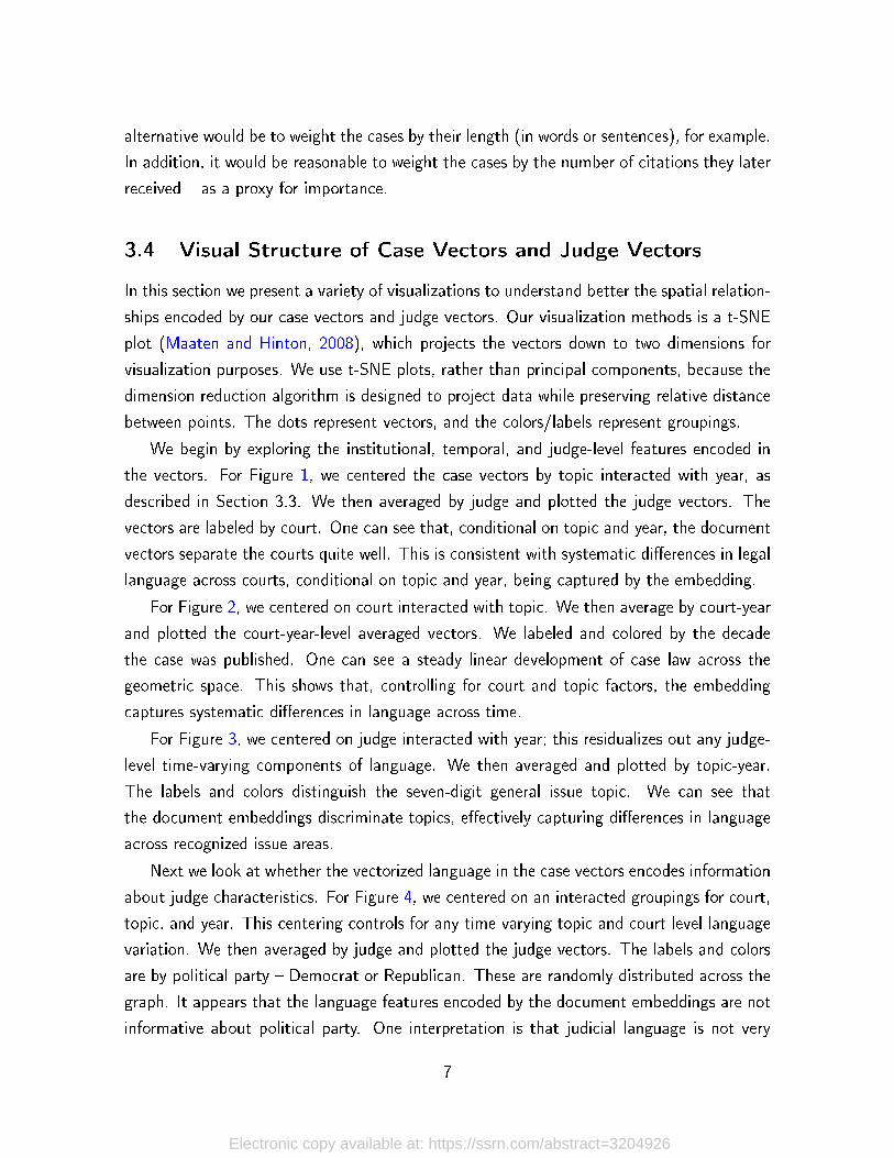
We begin by exploring the institutional, temporal, and judge-level features encoded in
the vectors. For Figure 1, we centered the case vectors by topic interacted with year, as
described in Section 3.3. We then averaged by judge and plotted the judge vectors. The
vectors are labeled by court. One can see that, conditional on topic and year, the document
vectors separate the courts quite well. This is consistent with systematic di�erences in legal
language across courts, conditional on topic and year, being captured by the embedding.
For Figure 2, we centered on court interacted with topic. We then average by court-year
and plotted the court-year-level averaged vectors. We labeled and colored by the decade
the case was published. One can see a steady linear development of case law across the
geometric space. This shows that, controlling for court and topic factors, the embedding
captures systematic di�erences in language across time.
For Figure 3, we centered on judge interacted with year; this residualizes out any judge-
level time-varying components of language. We then averaged and plotted by topic-year.
The labels and colors distinguish the seven-digit general issue topic. We can see that
the document embeddings discriminate topics, e�ectively capturing di�erences in language
across recognized issue areas.
Next we look at whether the vectorized language in the case vectors encodes information
about judge characteristics. For Figure 4, we centered on an interacted groupings for court,
topic, and year. This centering controls for any time-varying topic and court level language
variation. We then averaged by judge and plotted the judge vectors. The labels and colors
are by political party � Democrat or Republican. These are randomly distributed across the
graph. It appears that the language features encoded by the document embeddings are not
informative about political party. One interpretation is that judicial language is not very
7

Electronic copy available at: https://ssrn.com/abstract=3204926
Figure 1: Centered by Topic-Year, Averaged by Judge, Labeled by Court
DCDCDC
2
DCDC
DC
7
DC
8
5
DC
4
5
107
1
10DC DC
2
11
6
7611
FC
DC1
5
7
FC
FC FC
1
FC
FC
FC2
FC
FC
FC
FCFC
FC
FC
FC
11
FC
FC
FC FCFCFC
FC
FC FC
3FC
FC
FC
FC
FC FCFC
FC
FC
FC
FC
9
FC
FC
FCFC FC
FC
FC
4
FC
FCFC
FCFC
FCFC
FC
FC
FC
FC
FC
FC
FC
FC
FCFC
FCFC
FC
FC FC
11
11
11
11
11
11
5
11
1111
11
5
11
5
11
5
5
11
11
5
5511
11
11
11
5
5
11
5
11
11
5
11
5
5
5
11
11
11
11
11
11
5
115
5
11
1111
11
5
11
11
11
1111
5
5
11
11
1111
11
11
11
11
5
11 5
11
6
5
5
5 1111
5 2
11
11
11
11
11
11
5
11
11
11
5
5
11
7
11
11
11
11
11 5
11
11511
5
11
5
5
5
11
5
11
6
11
5
5
11
11
11
11
5
11
11
11
5
11
5
11
11
11
101010
10
10
1010
10
10 10
10
10
10
1010
10 10
10
10
10
10
1010
10
10
1010
10
10
10
9
1010
10
10
10
10
10
10
1010
10
10
10
10
10
10
8
10
1010
1010
1010
10
8
10 108
10 1010
10
8
10
10
10
10
10
10108
1010
10
8
10
10
10
10
10
10
10
10
10
1010
10
10
8
10
10
10 10
10
10
10
10
10
8
10
810
10
10
10
1010
10
10
10
10
1010
8
10
10
10
10 10
10
10
10
10
10
10
10
1010
9
9
9
9
4
9
9
9
99
9
9
9
9 9
9
9
9
9
9
99
9
9
9
9
9
99
9
9
9
9 99
9
9
9
9
9
9
9
99
9
9
9
9
2
9
9
9
99
9
9
9
9
9
9
9
9
9
9
999
9
9
9
9
9
9
9
9
99 11
9
9
9
9
9
9
9
9
9
9
9
9
DC
9
9
5DC
9
9
9
9
9
9
99
9
9
9
99
9
9
9
9
99
9
9
99
9
9
9
9
1
9
9
99
9
9
9
9
9
9
9
9
9
9
9
9
99
9
9
9
9
99
99 9
9
9
9
9
9
9
9
9
9
9
9
9
9 9
9
9
9
9
9
9
9
9
9
9
9
9
9
9
9
9
9
9
9
9
9
9
9
9
9
9
9
9
9
9
9
9
99
9
9
9
9
99
9
9
9
9
9
99
9
9
9
9
9
99
9 9
9
8
9
9
11
99 8
9
99
9
99
9
9
9
9
9
9
9
9
9
9
9
9DCDC9
9
9
9 9
9
9
9
99
9
9
9
9
9
9
9
9
9
9 9
9
9
11
9
9
9
9
9
9
9
9
9
9
9
9
99
9
9
9
9
9
9
9
9
9
9
9
9
9 9
9
9
99
9
9
9
9
9
99
9
9
9
9
9
9
9
9
9
97
9
99
9
9
9
99
8
8
8
8
8
8
8
8
88
88
8
8
88
8
8
8
888
8
8
8
8
8
8
8
8 88
8 8
88
8
8
8
8
8
8
88
8
8
7
8
8
88
8
8 88
8
8
888
8
8
8
888
88
8
8
8
8
8
8
8
8
8
8
8
8
8
8
88
8
8
8
8
8
8
8
8
8
8
8
8
DC
8
8
8
8
8
8
8
8
8
8
888
8
8
8
8
88
8
8
88
8
8
8
8
8
8
8
8
8
2
8
8
8
8
8
8
8
88
8
8
8
8
8
8
8
8
8
88
88
8
8
8
8
8
8
88
8
8
88
8
8
8
8
8
8
8
8 8
88
8
8
8
8
8
FC
9
8
8
8
8
88
8
8
8
8
8
8
8
88
8
8
88
8
8
8
7
77
7
7
7
7
7
7
7
7
7
7
77
7
7
7
7
7
7
7
77
7
7
7
1
DC
7
7
7
7
77
7
7
7
77
77
7
7
7
7
77
7
7
7
7 7
7
7
7
7
7
77
777
7
7
7
7
7
7
7
7
7
77
7
7
7
77
7
11
7
7
7
7
7
77
7
7
77
7
7
7
7
7
7
7
7
77
7
77
7
7
7
1
7
7
7
7
7
7
77
77
77
7
7
7
7
7
7
77
7
7
77
7
7
11
6
6
6
6
6
6
11
66
6 6
6
6
6
6
6
6
6
66
6
6
6
66
6
6
6
66
6
6
6 66
6
6
6
611
66
6
6
6
6
6
6
6
6
6
6
6
6
6
66
66
6
6
6
6
6
6
66
6
6
6
6
6
6
FC
66
6
6
6
6
6
6
6
6
6
DC
6 6
6
6
66
6
6
66
6
66
6
6
6
6
6
6
6
6
6
6
6
66
6
6
6
6
6
6
6
6
3
6
6
6
6
6
66
6
6
66
6
66
6
6
6
6
6
6
6
6
6
66 6
6
6
6
6
6
6
6
6
6
DC
6
6
6
6
6
6
6
6
66
6
6
6 6
6
6
6
6
6
6
6
6
66
6
6
6
6
6
6
6
6
6
8
66
6
6
6
6
6
6
6
6
6
6
6
6
6
6
6
6
6
6
6
6
6
6
6
6
6
6
6
6
6
6
6
FC
6
6
6 6
6
5
5
11
5
5
5
5
5
5 5
5
5
5
55
5
5
5
55
5
5
55
5
5
55
55
11
55
5555
5
7
5
5
5
5
5555
5
5
DC
5
5
5
5
5
5
5
5
5
5
5
5
5
555
5
5
5
11
5
5
5
5
5
55
5
11
5
5
5
5
5
5 5
5
5
5
5
5
5
5 5
5
5
5
55 5
5
5
5
5
5
5
5
5
5
5
11
5
55
55
15
5
DC
5
5 5
5
5
5
5
5
5
5
5
5
5
5
5
5
55
5
5
5
5
5
55
5
11
5
5
5
5
5
5
2
DC
5
5
5
5
5
5
5
2
10
5
5
5
5
5
5
5
11
5
5
5
5
7
55
55
5
5
5
5
FC
5
4
4
4
44
4
4
4
4
4
4
4
4
4
4
44 4
4
4
4
44
4
4
4
44
4
4
4
4
4
4
4
4
4
4
4
4
4
4
4
4
4
4 44
4
4
44
4 4
4
4
44
4
4
4
4
4
4
4
4
4
4 4
9
4
FC
4
4
11
44 4
4
4
44 4
4
4
4
4
4
7
4
4
44
4
4
4
4
4
44
44
44
FC
9
4
4
4 4
4
4
4
4
4
4
4
4
4
4
4
4
4
4
4
4
4
4
4
4
44
4
4
4
4
4
4
FC
4
4
4
4
4
4
4
4
44
4
4
4
4
4
4
4
4
4
44
44
4
4
4
4
4
4
4
4
4
4
4
4
4
4
4
4
44
4
4
4
4
44
3
3
333
3
3
3
3
3
3
3
3
7
113
3
3
DC
3
33 3
FC
3
3
3
3
3
3
3
3
3
3
3
1
3
11
33
3
33
3
3
3
3
3
7
3
3
3
33
3
3
3
3
33
3
33
3
3
3
3
3
6
3
3
3
3
3
3
3
33
3
3
3
3
3
3
33
3
3
3
3 DC3 3
3
33
3
5
3
3
33
3
33
3
3
DC
3
3
3
33
3
3
3
3
3
3
3
3
33
3
3
3
3
3 3
3
3
3
33
3
3
3
3
53
3
3
3
3
3
3
3
3
3
3
3
3
33
3
3
11
3
3
3
3
1 3
3
3
33
23
3
3
3
3
3
3
3
3
3
3
3
3
3
3
3
3 3
3
3
3
3
3
3
3
33
8
2 2
2
2
2
7
2
2
2
22
2
2
2
2
7
2
2
2
2
2
2
2
2
2
2
2
2
2
2
2
2
2
2
2
2
2
22
2
2
2
2
2
2
2
2
2 2
2
2
2
9
2
2
2
2
2
222
2
2
2
2
2 2
11
2
2
2
2
2
2
22
2
2
2
2
2
2
2
2
22
2
2
2
2
2
22
2 22 2
2
2
2
2
2
2
22 22
2
2
22
2
2
2
2
2
2
2
2
2
2
2
2
2
2
2
22
2
22
2
2
9
27
2
2
2
2
10 2
22
2
2
22
2 2
9
2
2
2
2
2
2
2
2 2
2
2
2
22
2
2
2
22
22
2
22
22
2
2
22
2
2
1
2
2
2
2
2
2
2
22
3
2
2
2
2
2 9
6
2
2
2
2
2
1
1
1
1
111
1
1
1
1
1
11
1
1
1
1
1
1
11
1
1
1
11
1
1
1 11
1 11
1
1
1
1 1
1
11
1
1
1
1
1
1
1
1
1 11
1
11 1
1
1
1
1
1
1
111
1
1
1 1
1
11
11
1
1
1
1
1
1
1
11
41
1
DCDCDC
DCDCDCDCDCDCDC3
DCDCDCDCDCDCDCDC
9
SCSCSCSCSCSCSCSCSCSCSCSCSCSCSCSCSCSC
SC
SCSC SCSCSCSC
SCSCSCSCSC
SC SCSCSCSCSC
−40
−20
0
20
40
60
−20 0 20 40
x
y
circuit
a
a
a
a
a
a
a
a
a
a
a
a
a
a
DC Circuit
Circuit−1
Circuit−2
Circuit−3
Circuit−4
Circuit−5
Circuit−6
Circuit−7
Circuit−8
Circuit−9
Circuit−10
Circuit−11
Federal Court
Supreme Court
Circuit, CC Judge Vector, Demeaned by Year and Big Topic
8

Electronic copy available at: https://ssrn.com/abstract=3204926
Figure 2: Centered by Court-Topic, Averaged by Court-Year, Labeled by Decade
2000s
2000s
1980s
1980s
1990s
1990s
1990s
2000s 2000s
2000s2010s
2010s
2000s2000s
2000s
2000s
2000s2000s
2010s
2000s
2000s
1910s
1990s
2000s
2010s
1980s
1910s
1990s
1910s
1980s
1920s
1920s1920s
1920s
1920s
1920s
1920s
1920s1920s
1920s
1910s
1920s
1910s1910s
1910s
1910s
1990s
1940s
1900s
1900s
1900s
1900s
1890s
1890s
1890s
1890s
1890s
1890s
1890s
1900s
1900s 1900s
1900s
1890s
1910s
1900s
1910s
1900s
1900s
1920s
1910s
1990s
2010s
1990s
2010s
2010s
1970s
2010s
2010s
2010s
2010s2010s
1980s
2010s
2010s
1980s
1990s
1990s
1980s
1980s1980s
1990s
1990s
1940s1940s
1970s
1930s
1930s1930s
1930s
1930s
1930s
1930s1930s1930s
1930s1930s
1960s1960s1960s1960s
1960s
1960s
1960s
1960s1960s
1960s
1960s
1930s
1990s
1950s
1950s1950s
1950s1950s
1950s
1950s1950s
1970s
1970s
1890s
1970s1970s
1980s
1990s
1970s
1970s1970s
1970s1970s1970s
1980s
1980s
1980s
1980s
1940s
1950s
1940s
1960s
1970s
1940s
1940s
1940s
1950s
1940s
1940s
1940s1940s
1950s1950s
1920s
1960s
1890s
1910s
1910s
1900s
1890s
1900s
1950s
1960s
1970s
1980s
1990s
2000s
1940s
2010s
1890s
1900s1910s
1920s
1930s
−10
−5
0
5
10
−10 −5 0 5 10
x
y
decade.s
a
a
a
a
a
a
a
a
a
a
a
a
a
1890s
1900s
1910s
1920s
1930s
1940s
1950s
1960s
1970s
1980s
1990s
2000s
2010s
Court Decade, SC & CC Court Decade Vector, Demeaned by Circuit and Big Topic
9

Electronic copy available at: https://ssrn.com/abstract=3204926
Figure 3: Centered by Judge-Year, Averaged by Topic-Year, Labeled by Topic
4
1
6
7
6
4
66
7
4
2
6
7
6
4
1
7
2
6
35
1
4
1
7
2
4
6
3
7
1
2
4
1
2
1
4
7
4
6
35
7
7
7
4
1
7
4
1
1
777
7
1
2
6
7
6
7
4
6
2
3
5
77
4
7
4
7
4
7
1
4
1
7
7
6
7
4
1
7
6
2
3
7
3
2
4
1
7
4
3
7
2
4
1
6
5
77
4
1
4
6
3
4
1
7
7
2
1
5
7
4
2
1
2
7
1
3
6
7
4
6
4
6
4
6
7 7
6
44
2
44
6
5
66 666
6
1
7
77
6
4
3
7
3
6
2
5
7
4
7
6
7
1
4
7
2
6
7
4
2
1
4
6
5
1
7
2
644
4
1
7
4
7
4
7
7
4
7
1
6
7
2
7
7
2
4
2
6
4
3
1
2
1
22
1
6
3
2
1
6
2
3
1
4
7
4
7
44
1
2
4
3
777
4
77
4
777
1
77
4
1
4
77
4
1
7
4
7
1
7
7
7
1
7
4
7
11
7
2
1
4
1
4
77
1
7
4
6
1
4
1
6
4
2
4
7
1
7
4
7
4
11
7
7
4
11
4
7
2
4
1
7
4
1
6
7
1
6
4
11
4
6
3
6
1
7
1
7
2
3
6
44
2
6
1
7
3
4
7
1
4
1
1
4
77
7
7
6
7
44
7
5
6
3
2
7
1
3
1
4
6
7
7
5
1
4
2
4
5
3
4
1
2
6
1
3
66
2
6
3
22
35
2
3
2
3
5
3
2
3
2
1
5
3
2
353
22
3
5
33 3
5
2
1
33
5
5 3
555 5
44
1
2
1
6
4
1
2
7
6
4
1
3 2
4
2
1
4
2
6
2
7
4
1
66
2
6
1
4
2
4
1
6
2
1
7
4
4
1
23
6
6
2
1
4
6
2
3
7
1
6
2
1
6
2
4
4
6
1
2
3
1
6
2
5
2
1
4
6
3
1
4
7
6
2
4
7
1
2
1
4
7
6
2
1
6
66
222
1
6
2
2
6
3
5
2
1
6
3
2
3
2
6
3
6
3
2
6
2
3
6
2
5
6
2
3
2
4
1
5
2
6
5
7
2
64
1
6
22
4
2
6
1
55
6
1
2
4
2
6
2
6
6
3
5
3
6
2
35
5
6
4
1
2
5
3
3
2
55
3
33 33 33
6
2
35
35
535 3
3
5
3
5
1
2
3
3
333
53
3
3
55
3
5
3
5
7
11
44 6
1
2
11
4
46
11
64
7
4
1
6
7
2
1
7
4
1
7 1
4
11
11
77
4
1 1
6
4
3
35
1
6
77
4
4
6
3
2
7
6
6
3
1
6
2
66
7
2
44
1
6
2
6
2
2
6
2
6
2
64
3
3
22
6
2
1
3
6
22
4
2
6
7
4
2
1
2
6
2
66
2
1
4
2
6
2
66
1
3
6
23
71
2
6
2
4
2
3
6
3
6
5
1
5
−50
0
50
−25 0 25
x
y
big.issue
a
a
a
a
a
a
a
1 − Criminal Appeal
2 − Civil Rights
3 − First Amendment
4 − Due Process
5 − Privacy
6 − Labor
7 − Regulation
Big Topics and Year, SC & CC Topic Year Vector, Demeaned by Judge and Year
10

Electronic copy available at: https://ssrn.com/abstract=3204926
politicized (related to the result in Ash et al. (2017) that judicial language is less polarized
than congressional language). Another possibility is that our representation of language
is not rich enough to encode ideological content. Richer representations, such as those
constructed from grammatical relations between words (Levy and Goldberg, 2014), may be
needed.
Figure 5 considers another judicial biographical feature: birth cohort. As before, we
centered on court-topic-year and averaged/plotted by judge. In this case, the labels and
colors are by birth cohort decade (1910s through 1950s). In stark contrast to political party,
there is clear segmentation across the geometric space across cohorts. Remember that this
is conditioned on court-topic-year, so is not driven by time trends over the sample. The
vectorized language recovers di�erences in the legal language used by judges from di�erent
generations.
Finally, for Figure 6, we consider law school attended as a �nal source of linguistic
di�erences across judges. Conditional on court, topic, and year, we see apparent random
distributions across the space in terms of law school. As with political party, it seems like
language or ideological di�erences by school do not show up in the vectors. Again, this may
be due to ideologically distinctive embeddings requiring a richer representation of language
than that used here.
3.5 Analysis of Relations Between Judges
This section uses our vector representation of judges to produce a similarity metric between
courts and judges. We adopt a measure of vector similarity that is used often for document
classi�cation. The cosine similarity between two vectors,
s(~v, ~w) =~v · ~w‖~v‖ ‖~w‖
,
which is equal to one minus the cosine of the angle between the vectors. It takes a value
between -1 and 1. In the case of word embeddings, high similarity means that the words
are often used in similar language contexts.
In the case of judges, we can say that similarities approaching one mean that the judges
tend to use similar language in their opinions. Similarities approaching -1 meaning the judges
rarely use the same language. Similarities near zero mean that the judges are as similar to
each other as would be expected from two randomly selected judges in the population.
First we look at similarity between court vectors to complement the spatial representation
11

Electronic copy available at: https://ssrn.com/abstract=3204926
Figure 4: Centered by Court-Topic-Year, Averaged by Judge, Labeled by Political Party
D
R
D
R
R
RR
R
D
R
R
D
R
R
D
R
D
R D
D
RRR
R DD
R
R
R
R
D
R
D
D
D
D
D
D
R
R
D
R
D
D
R
R
R
R
R
R
R
R
R
D RR
R
D
R
D
R
R
D
R
D
R
R
R
D
D
R
R
R
D
D
R
D
R
R
D
R
RR
R
R
R
R
RR
D
D
R
R
D
R
D
R
R
D
R
R
R
R
R
R
D
D
D
R
R
D
R
R
D
D
R
R
DR
R
R
D
D
R DD
R
DR
R
R
R
R
D
R
D
R
R
D
R R
R
R
D
R
R
R
D
R
R
R
R
R
R
R
R
R
D
R
R
D
RD
D
R
R
R
R
D
R
R
D
R
D
D
RR
R
RD
R
R
R
D
RD
D
D
R
DRD
R
R
D
R
D
D
R
D
RR
D
R
D
D
R
D
D
D
R
D
R R
D
R
R
R
R
D
D
R
R
D
D
R
R
R
RR
DDR
R
D
R
R
DR
D
RR
R
R
R
R
R
R
R RD
R
D
R
R
R
R
R
R
RR
R
R
R
R
D
R
R
R
D
D
D
D
R
R
R
R
D
R
R
R
R
R
D
R
D
DD
R
R
R
D
D
D
R
R
D
R
R
R
D
D
R
R
R
D
R
R
R
D
R
R
D
R
D
R
D
D
D
R
R
D
R
R
R
R
R
D
R
R
R
R
D
D
R
R
R
R
D
R
R
R
R
R
R
R
D
D
R
R
R
R
D
R
R
R
R
R
D
R
R
D
R
DR
R
D
R
R
D
D
D
RR
R
DR
R
R
R
R
DR D
D
D
D
R
R
D
D
R
R
R
D
D
D
R
D
D
D
R
R
D
D
RD
R
R
D D
R
D
DR
D
R D
D
R
D
D
D
D
D
D
D
R
D
R
D
D
D
D
D
R
D
D
R
R
D
R
R
D
D
D
R
D D
D
R
D
D D
D
D
D
D
D
R
R
R
D
R
D
R
D
R
R
R
D
R
D
R
D
R
D
D
R
D
RR
R
R
R
D
D
D
D
D
D
D
D
R
D
D
R
R
RR
D
D
R
D
RD
R
R
R
R
R
R
D
D
R
RR
D
D
D
R
R
D
D
D
R
D
R
D
R
D
R
R
R
R
D
D
R
D
D
R
D
R
R
D
D
R
R
R
R
R
R
D
D
RR
R
D
D
D
D
R
D
R
R
R
D
R
D
D
R
R
R
R
R
R
R R
R
R
R
R
R
R
R
D
R
D
D
D
R
D
R
R
D
D
R
DR
R
RR
R
D
R
D
R
R
D
R
D
R
D
R
RR
D
R
R
D
D
R
D
D
D
R
D
R
R
R
D
R
R
D
R
RD
D
R
D
R
R
R
R
R
R
D
R
D
D
D
R
D
R
R
D
R
RD
D
R
D
R
D
D R
R
D
R
D
R R
D
R
RD
R
R
R
R
D
D
D
R
D
D
R
D
R
DD
D
D
D
R
D
R
D
R
D
R
D
R
D
R
D
D
R
D
D
R
R
R
R
R
R
D
D
R D
R
R
DR
D
R
D
D
R
D
R
R
D
D
R
D
D
R
D
D
D
D
R
D
R
R
D
D
R
DD
D
D
D
D
D
D
D
R
D
R
D
R
D
D
D
D
R
D
R
R
R
R
R
R
D
R
D
D
R
D
R
R
R
D
D
R
R
D
R
D
R
R
D
D
R
DD
R
D
R
D
D
D
D
D
DD
R
R
D
R
D
RRR
R
D
D
D
D D
R
D
D
R
D
R
R
R
R
D
RR
R
D
R
D
D
R
R
R
R
D
R
R
D
D
D
D
D
R
R
DD
D
R
D
D
D
D
R
R
R
D
D
RD
D
D
R
R
R
D
R
R
R
R
R
D
D
R
R
D RR
R
D
D
D
D
D
R
D
D
D
D
D
D
D
D
D
D
D
D
R
D
R
D
D
D D
D
R
D
D
R
D
D
R
R
D
R
R
D
R
R
R
R
R
D
R
R
R
R
R
R
D
R
R
R
R
D
D
R
R
D
R
D
R
D
R
R
R
R
D
R
R
R
R
R
D
R
R
R
R
D
R
D
R
D
D
R
D
D
D
R
D
R
R
R
D
R
R
R
R
R
R
R
R
D
R
D
R
R
R
R
R
R
D
R
R
R
R
D
D
R
R
R
D
D
R
R
R
D
D
R
R
R
R
R
RD
R
D
R
D
R
D
R
R
R
R
R
D
R
D
D
D
R
D
D
D
D
R
R
R
R
R
R
D
R
D
R
D
R
D
D
D
R
R
D
D
R
D
R
R
D
D
D
R
R
D
R
D
R
D
D
D
R
R
D
R
R
D
R
R
D
D
R
D
D
D
R
D
D
R
R
R
R
D
RRR
R
R
D
R
R
R
R
R
R
R
D
R
D
R
D
R
D
D
R
D
D
R
D
R
D
R
R
D
R
D
D
R
D
D
D
R
R
R
D
R
D
R
D
D
D
D
D
D
R
R
R
R
R
R
D
R
R
D
R
R
D
R
R
R
D
R
R
D
R
R
D
R
R
R
R
R
R
R
R
R
R
R
D
R
R
R
D
R
R
D
R
R
DD
R
R
D
D
R
R
R
D
D
D
R
R
D
R
D
D
R
R
D
D
D
D
R
R
R
R
R
D
DR
RR
D
R
R
R
R
R
R
R
R
R
R
D
R
D
D
R
R
R
R
D
R
D
DR
R
R
R
D
D
D
R
D
D
D
D
D
D
D
D
D
D
R
D
R
R
D
R
D
D
R
D
D
R
R
DD
D
D
D
D
R
R
R
R
D
D
D
D
D
R
D
R
R
D
D
D
DR
D
R
R
D
D
R
DD
D
D
D
D
D
D
D
DD
D
R
DD
D
R
D
D
R
D
D
R
R
R
D
R
R
R
R
R
D
R
D
R
D
D
R
R
R
D
R
RD
D
D
D
R
R
R
R
RR
D
D
R
R
R
D
R
D
D
D R
D
D
R
R
D
D
R
R
D
R
RD
DR
D
D
D
D
D
D
D
D
D
R
D
D
D
D
D
D
R
D
D
D
R
RD
D
R
R
R
R
D
R
R
R
D
D
D
R
R
D
D
D
D
DD
R
R R
R
D
D
D
D
RR
D
R
R
R
R
R
R
R
R
R
D
DD
D
D
R
R
R
R
R
R
R
R
D
R
R
D
D
D
R
D
R
R
R
D
D
R
D
D
D
D
D
R
D
R R
D R
R
R
R
R
D
R
R
R
R
D
R
R
R
R
R
D
R
D
D
R
D
R
R
D
D
D
D
D
R
D
D
R
D
R
R
R
R
D
R
R
DR
R
R
R
R
R
D
R
R
R
R
R
R
R
R
D
R
R
R
R
R
D
R
R
R
D
D
R
D
R
D
D
R
D
R
R
D
R
D
D
R
D
R
D
R
DR
R
R
R
D
D
R
D
R
R
D
DR
R
D
D
D
D
R
D
R
D
R
R
R
D
D
D
D
D
R
D
R
D
RD
D
R
R
R
D
D
R
D
R
D
D
D
D
D
D
D
R
R
R
D
R
R
R
R
R
R
R
R
D
D
D
R
R
D
R
D
R
RR
R
R
D
D
R
R
D
D
D
D
R
R
D
D
R
D
R
R
R
D
R
R
D
R
D
R
D R
D
R
D
D
D
D
R
D
D
R
D
D
R
D
D
DR
D
R
R
D
R
R
D
D
D
D
D
R
D
D
D
D
D
D
D
D
R
R
D
D
R
R
D
D
R
R
R
R
D
D
R
R
D
D
R
D
R
R
R
R
R
D
D
DD
D
D
D
R
D
D
D
D
D
R
D
R
D
D
R
D
D
D
R
R
R
R
R
R
R
R
R
D
D
D
D
D
D
D
D
R
R
R
D
D
D
D
D
D
D
D
D
D
D
R
D
D
R
R
R
D
R
R
D
R
D
D
R
D
D
D
D
D
R
R
D
R
R
D
R
R
R
D
R
R
D
D
D
D
D
R
D
D
D
D
D
D
R
R
R
R
R
D
R
R
R
R
D
D
D
R
D
D
D
D
D
D
D R
R
R
R
R
R
D
R
D
R
R
D
D
R
R
R
R
RD
D
D
R
R
D
D
D
R
R
R
D
D
D
D
D
D
D
D
R
R
R
D
R
R
R
D
R
R
D
D
R
R
D
D
D
D
D
D
R
D
D
D
D
R
D
D
D
D
D
D
DDR
D
D
D
R
D
D
R
D
R
R
D
R
R
R
D
RR
R
R
D
R
R
D
R
R
R
R
D
D
R
R
R
R
R
D
R
D
D
R
D
R
D
D
R
D
D
D
R
D
D
D
D
D
D
D
R
R
R
D
R
D
R
R
RR
R
R
R
D
R
D
D
R
D
R
R
R
R
D
R
R
R
D
R
D
D
R
R
R
R
R
R
R
R
R
R
R
D
R
R
R
DR
R
R
R
R
RR
R
R
R
R
R
R D
D
R
D
R
D
R
R
R
R
RR
R
R
R
D
R
R R
R
R
D
D
R
D
D
R
R
D
D
D
D
D
R
D
D
R
R
DR
R
D
R
R
R
R
RR
R
R
R
R
R
R
R
R
R
D
R
R
RR
R
R
R
RR
R
D
R
R
R
R
R R
R
R
R
R
R
D
R
R
R
R
RR
R
RD
R
R
−30
−20
−10
0
10
20
30
−30 −20 −10 0 10 20 30
x
y
party
a
a
Democratic
Republican
Party Affiliation, SC & CC Judge Vector, Demeaned by Circuit, Big Topics, and Year
12

Electronic copy available at: https://ssrn.com/abstract=3204926
Figure 5: Centered by Court-Topic-Year, Averaged by Judge, Labeled by Judge Birth Cohort
50s
50s50s
20s
40s
50s
30s20s
40s
30s
20s
20s
40s
40s
50s
20s
40s30s
30s
30s
40s
20s
50s
30s
40s
20s
30s
30s
50s
30s
30s
50s
30s
20s
30s
40s
20s
50s
10s
20s
20s
50s
30s
40s50s
40s
20s
40s
10s10s
10s
10s
20s
50s
40s
50s
10s
10s
10s
10s10s
10s
20s
30s
20s
10s
10s
10s
10s
20s
10s
10s20s
10s
10s
10s
10s
20s
10s
10s10s
20s
10s
20s
10s
10s
10s
10s
10s
30s
20s
20s
10s
40s
20s
10s
20s
10s
10s
30s
10s
20s
10s
10s
30s
10s
20s
40s
20s
20s
30s
20s
40s
30s
20s
20s
10s
30s
30s
40s
30s
30s
20s30s
30s
40s
50s 30s
20s
30s
30s30s
40s
40s
50s
50s
20s
40s
40s
10s
20s
30s
30s
40s
40s
30s
50s
40s
30s
20s
10s
40s
40s
30s
10s
40s
30s
20s
40s
20s
40s
20s
40s
40s
10s
10s10s
40s
40s
50s
30s
40s
20s
40s
10s
10s
10s
10s
10s
30s
10s
20s
10s
10s
10s
20s
30s
30s
10s
30s
10s
20s
20s
10s10s
40s
30s
40s
40s
20s
40s
10s
10s
10s
10s
20s
20s
20s
40s
20s
30s
10s
10s
10s
50s
40s
20s
20s
10s
10s20s
10s
10s
10s
20s
10s
20s
40s
10s
10s
10s
20s
30s
40s
10s
10s
10s
10s
10s
20s
30s
20s
40s
50s
20s
20s
40s
50s
50s
30s
40s
40s
20s
30s
30s
40s
30s
30s
40s
50s
40s
20s
40s
30s
50s
30s
30s
40s
30s
20s
30s
50s
10s
30s
40s
20s
30s
10s
10s
40s50s
50s
10s
10s
10s
20s
30s
10s
50s
10s
30s
50s
40s
30s10s
20s
10s
10s
10s
20s
10s
10s10s
10s
10s
10s
30s
20s10s
20s
20s
30s
40s
10s
30s
20s
10s
40s
20s
40s
50s
30s
40s
30s
20s
40s
10s
40s
40s
50s
10s
20s
20s
30s
40s
40s
40s
40s
20s40s
40s
20s
40s
50s
20s
30s
30s
40s
30s
20s
30s
40s
40s
30s10s
20s
10s
30s
10s10s
10s
10s
10s
20s10s
10s
20s
10s
50s
30s
40s
10s
30s
10s
20s
20s
10s
20s
30s
20s
30s
20s
30s
50s
50s
40s
30s
20s
50s
50s
20s
50s30s
30s
20s
40s
50s
30s40s
40s
20s
40s
40s
50s
30s
20s
50s
40s
50s
40s50s
10s
10s
10s
10s
10s20s
10s
10s
10s10s
10s
10s
20s
10s
20s 10s
20s
30s
10s
20s
30s
20s
30s
30s
30s
40s
30s
30s
10s
30s
20s
40s
20s
10s
30s
20s
40s
10s
40s
30s20s
30s
30s
10s
20s
10s
10s
10s
20s
10s
10s
10s
10s
10s
10s
20s
20s
10s
40s
40s
40s
20s
20s30s
20s
20s
20s
30s
40s
30s
30s
40s40s
50s
40s
40s
40s
20s
50s
50s
40s
30s
20s
30s
20s
30s
30s
40s
50s
50s
10s
10s
20s
50s
40s
50s
50s
50s
50s
50s
20s
40s
10s
20s
40s
30s 20s
30s
30s
50s
10s
10s
10s
20s
30s
10s
10s
10s
20s
10s
30s
10s
40s
10s
40s
20s
10s
10s
10s
20s
40s
40s
40s
30s
20s
40s
40s
20s
20s
30s
40s
30s
30s
50s
20s
30s
30s
20s
20s
40s
30s
40s
30s
40s
20s
30s
20s
40s
30s
20s
20s
40s
20s
40s
10s
10s
30s
50s
50s
30s
50s
40s
40s
40s
10s
10s
10s
10s
20s
20s
20s
10s
20s
30s
20s
40s
20s
10s
20s
30s
30s
10s
30s
40s
10s
20s
30s
50s
10s10s
10s
10s
10s
10s
10s
10s
10s
30s
40s
50s
40s
40s
40s
30s
50s
30s
20s
40s
40s
30s
30s
30s
40s
30s
30s
40s
30s
50s
30s
20s
40s
40s
30s
30s40s
20s
40s
20s
20s
50s
30s
30s
20s
50s
30s
50s
10s
10s10s
10s
30s
40s
10s
30s
30s
20s
10s
20s
10s
20s
20s
10s
20s
20s
30s
10s
10s
10s10s
10s
10s
10s
20s
30s
10s
10s
10s
20s
40s
50s
40s
30s30s 30s
20s
30s
20s
10s
20s
40s
40s
10s
50s
20s
30s
40s
50s
40s
20s
30s
20s
40s
50s
20s
40s
40s
40s
40s
10s
10s
10s
10s
10s
10s
10s
20s40s
10s
50s
30s40s
30s
30s
30s
50s
40s
20s
10s
10s
40s
10s
20s
40s
30s
10s
10s
30s
10s10s
10s
30s
10s
10s
20s20s
40s
50s
20s
10s
40s
40s
40s
50s
50s
50s
50s
30s
20s
30s
20s
20s
20s
40s
50s
40s
40s
30s
40s
40s
20s
40s40s
40s
50s
40s
50s
50s
50s
50s
40s
50s40s
20s
20s
10s
50s50s
40s
10s
40s
10s
20s
10s
10s
20s
10s
20s
10s
20s
10s
10s
10s
10s
40s
10s
40s
40s
30s
30s
20s
30s
40s
20s
40s
40s
20s30s
10s
20s
30s20s
10s
20s40s
20s
20s
40s
10s
40s
20s
40s
40s
40s
40s
10s
30s
40s
10s
10s
10s
10s
50s
40s
10s
10s
20s
10s
10s
10s
20s
30s
20s
30s
20s
20s20s
40s
50s
40s
10s
30s
10s
20s
10s10s
10s
10s20s
20s
20s
10s
20s
20s
20s
20s
30s
10s
40s
40s
20s
20s
40s
30s
20s
50s
20s
20s
20s
30s30s
40s
40s
40s
30s30s
50s
30s
30s
10s
50s
40s
40s
30s
40s
10s
40s
20s
40s30s30s
20s
40s
40s
50s
40s
40s
40s
20s
50s50s
50s
20s
10s
20s
30s
10s
10s
10s
10s
10s
10s
10s20s
10s
10s
20s
10s
20s
20s
20s
10s
20s
30s
20s
10s
30s
20s
20s
30s
30s20s
20s
40s
40s
20s
40s
10s
30s
10s
10s
10s
10s
10s
30s
20s
10s
10s
10s
30s
30s
20s
10s
10s
10s
10s
20s
10s
10s
20s
30s
20s
20s
20s
20s
10s
10s
20s
10s
10s
10s
20s
10s
30s
10s
10s
10s10s
10s
10s
10s
10s
20s
10s
20s
40s
10s
10s
40s
40s
40s
50s
40s
50s
50s
40s
20s
40s
50s
30s
30s
30s
30s
30s
40s
30s
30s
40s
30s30s
20s
30s
30s50s
20s
30s
40s
30s
40s
20s
30s
30s
20s
50s
50s40s
40s
40s
40s
50s
40s
30s
50s
50s
40s
50s
50s
10s10s
10s
10s
10s10s
10s
20s
50s
40s
40s
40s
30s
10s
30s
40s
10s
10s
10s
10s
10s
20s
10s
30s
20s
20s
10s
20s
10s
10s20s
20s
10s
10s
10s
30s
10s
20s
20s
10s
10s
40s
10s
10s
20s
10s
10s20s
20s
20s
30s
10s
30s
30s
30s
20s
20s
20s
10s
30s
20s
30s
20s
20s
50s
30s
30s
10s
40s
40s
30s
20s
20s
30s
20s
50s
30s
40s
20s
10s
50s
20s
40s
30s
40s
30s
10s
10s
20s
10s
20s
40s
50s
10s
20s
10s
10s
30s
40s
10s
10s30s
10s
10s
10s
10s
10s
10s
20s
30s
20s
10s
20s
30s
40s
30s
40s
40s
50s
40s
40s
50s
40s
30s
40s
40s
50s
50s
50s
10s 20s
40s
20s
20s
10s
10s
10s
10s
10s
10s
20s
30s
20s
20s
10s
40s
40s
40s
50s
30s
30s
40s50s
30s
30s
40s50s
40s
40s
10s
20s
10s
10s10s
20s
30s
10s
10s
20s
10s
10s20s
10s
40s
20s
10s
30s
10s10s
20s
10s
40s
20s
30s
10s
10s
20s
10s
10s
10s
10s
10s
20s
10s
10s
10s
10s
30s
30s
40s
20s
30s
30s
40s
40s
50s
20s
40s
20s
50s
40s
40s
50s
30s
10s
10s
10s
20s
10s
10s
10s10s
10s
10s
20s
20s
20s
20s
10s
20s
10s
30s
10s
20s 10s
40s
30s
40s
10s
20s
30s
30s
40s
20s
10s
50s
50s
20s
40s
30s
40s
10s
30s
30s
30s
50s
20s
10s
50s
50s
10s
10s
10s
10s20s
20s
20s
30s
30s
40s
20s
40s
50s
20s
10s40s
30s
10s
10s
30s
10s
40s
30s
30s
40s
40s
30s
30s
50s
30s
20s
30s
20s
40s
40s
20s
40s
40s
20s
40s
50s40s
40s
50s
20s
50s
40s
40s
30s
30s
40s
40s
30s
20s
40s
40s
30s
20s
10s
20s
20s
50s
10s
10s
10s
10s
20s
10s
10s
40s
10s
50s
20s
10s
10s
20s
10s
30s
10s 10s
20s20s
20s
30s
20s
30s
10s
40s
20s
30s
40s
40s
20s
30s
30s
30s20s
40s
10s
20s
30s
10s
30s
20s
40s
20s
30s
30s
20s
40s
50s
10s
40s
10s
30s
10s
10s
10s
10s
20s
30s
10s
50s
50s
20s
40s
10s
10s
10s
30s
40s
50s
50s
10s
30s
30s
30s
40s
50s
40s
20s
30s
20s
50s
50s
10s
40s
10s
30s
20s
10s
30s
10s
20s
10s
30s
20s
30s
40s
20s
40s
40s
30s
40s
30s
10s
50s
40s
20s
30s
20s
20s
40s
40s
50s
30s
30s50s
40s 10s
30s
40s
10s
20s
10s
40s40s
40s
30s
50s
20s
50s
30s
30s
20s
40s
40s
30s
40s
40s
40s
40s
30s
20s
40s
50s
50s
30s
−20
−10
0
10
20
−30 0 30
x
y
cohort
a
a
a
a
a
1910s
1920s
1930s
1940s
1950s
Cohort, CC Judge Vector, Demeaned by Circuit and Big Topic
13

Electronic copy available at: https://ssrn.com/abstract=3204926
Figure 6: Centered by Court-Topic-Year, Averaged by Judge, Labeled by Law School At-tended
−30
−20
−10
0
10
20
−20 −10 0 10 20 30
x
y
law_sch
Columbia Law School
Harvard Law School
Stanford Law School
University of Chicago Law School
University of Michigan Law School
University of Pennsylvania Law School
University of Texas School of Law
University of Virginia School of Law
Yale Law School
Law School, SC & CC Judge Vector, Demeaned by Circuit, Big Topics, and Year
14

Electronic copy available at: https://ssrn.com/abstract=3204926
Table 1: Pair-Wise Similarities Between Federal Appellate Courts
SCOTUS 11.th Circ. D.C. Circ. Fed. Circ.
SCOTUS 1.000
0.022 1.000
-0.008 0.302 1.000
-0.001 0.135 0.207 1.000
-0.045 -0.045 -0.081 0.126 1.000
-0.105 -0.196 -0.298 -0.269 0.038 1.000
-0.074 -0.185 -0.148 0.009 0.069 -0.107 1.000
-0.097 -0.052 -0.014 -0.055 -0.162 -0.257 0.029 1.000
-0.137 -0.215 -0.296 -0.214 -0.150 -0.184 0.050 -0.022 1.000
0.039 -0.137 -0.140 -0.182 -0.147 -0.121 -0.220 -0.265 -0.150 1.000
-0.111 -0.249 -0.361 -0.179 -0.189 0.017 0.006 -0.158 0.218 0.042 1.000
11.th Circ. -0.086 -0.191 -0.240 -0.215 0.067 0.713 -0.039 -0.224 -0.192 -0.084 0.026 1.000
D.C. Circ. 0.846 -0.085 -0.058 0.011 -0.010 -0.062 -0.097 -0.177 -0.111 0.067 -0.025 0.011 1.000
Fed. Circ. 0.178 0.200 0.132 0.116 0.124 -0.150 -0.154 -0.082 -0.255 -0.116 -0.260 -0.181 0.094 1.000
1st Circ. 2nd. Circ. 3rd. Circ. 4th Circ. 5th Circ. 6th Circ. 7th Circ. 8th Circ. 9th Circ. 10th Circ.
1st Circ.
2nd. Circ.
3rd. Circ.
4th Circ.
5th Circ.
6th Circ.
7th Circ.
8th Circ.
9th Circ.
10th Circ.
in Figure 1. We centered the vectors by topic and year, and then aggregated by court. We
then computed the pair-wise similarities between the court vectors. These are reported in
Table 1.
The colors provide a gradient for similarity, with green meaning the courts are relatively
similar and red meaning they are relatively dissimilar. The table has some interesting fea-
tures. First, the D.C. Circuit is most similar to the Supreme Court of the United States,
which is intuitive since they are both located in Washington, D.C. and focus on issues of
federal government functioning such as separation of powers. Second, the 11th circuit is
similar to the 5th circuit, which is intuitive since the 11th Circuit used to be a part of the
5th Circuit and they share many legal precedents.
Next we look at similarity between judge vectors. Starting with the Supreme Court,
we center the document vectors on topic, and year. Then we take the average of these
centered vectors by judge as our representation of judge writing, reasoning, and beliefs.
Table 2 (continued in Table 3) reports the pair-wise similarities between a selection of
recently sitting Supreme Court judges. Overall, there are limited immediate insights and
the results are mixed. For example, it is intuitive that Scalia is close to Thomas. But
counter-intuitively, Scalia is even closer to Souter, Stevens, and O'Connor. Another example:
Intuitively, Brennan is close to Thurgood Marshall; but counter-intuitively, he is closer to
White and Stewart. Overall, the judge vectors do not seem to encode similarities between
Supreme court judges very well. This may be due to the relatively few decisions that they
author. In particular, the relative dissimilarity between Kagan and most other justices is
15

Electronic copy available at: https://ssrn.com/abstract=3204926
likely due to her having only a handful of decisions in the corpus.
One interesting feature of our model is that it represents both circuit court judges and
supreme court judges in the same geometric space. As done previously, we center all the
document vectors on court, topic, and year. We then aggregate by judge. For Table 4, we
computed the vector similarity between each circuit court judge and each supreme court
judge. We then ranked the circuit court judges by this similarity. The table shows, for
each supreme court judge, the top 5 circuit court judges on this ranking. As with the pair-
wise similarities between supreme court judges, these rankings are not particularly intuitive
or informative. Understanding the limitations of these types of models is important for
future research. An important factor is that we use a bag-of-words model, and ideological
di�erences between judgs may be mostly encoded in phrases.
A possible reason for the lackluster results in the Supreme Court is that the justice vec-
tors may not be well de�ned due to the small number of opinions they publish. Therefore
we round out this analysis by looking at a notable circuit court judge, Richard A. Posner.
The document vectors are de-meaned by court, year, and topic. Then they are aggregated
by judge. Then we rank all circuit court judges by the similarity of their vector to Posner's
vector. These are reported in Table 5. Interestingly, the most similar judge is Frank East-
erbrook, who, like Posner is known for the use of economic analysis in opinions. Stephen
Breyer has a published article in The Economic Journal on �economic reasoning and judicial
review� (Breyer, 2009). Posner has a conservative reputation, and we see other conservative
judges such as Neil Gorsuch and Antonin Scalia. Henry Friendly makes an appearance � he
is a well-known pragmatist, as is Posner. Finally, Michael McConnell co-write law articles
with Posner. The document vectors, as trained in this example, are much more informative
about the connections between circuit court judges than between Supreme Court judges.
4 Discussion of Parallel and Future Work
We conclude with a discussion of how future work could adapt these embeddings models
for empirical analysis of law.
4.1 Structured Group Embeddings
The document embeddings developed in the previous section were static, and did not ex-
plicitly model a time component. In addition, they only encoded judge identity by taking
the average of a judge's document vectors. Recent work in embeddings models seeks to
16

Electronic copy available at: https://ssrn.com/abstract=3204926
Table2:
Pair-WiseSimilarities
betweenSuprem
eCourtJudges
AFortas
AMKennedy
AScalia
BRWhite
CThomas
DHSouter
EKagan
EWarren
FFrankfurterFMVinson
HABlackmun
HLBlack
JGRoberts
JPStevens
AFortas
1.0
00
AMKennedy
0.7
33
1.0
00
AScalia
0.7
35
0.9
74
1.0
00
BRWhite
0.8
34
0.9
08
0.9
13
1.0
00
CThomas
0.6
86
0.9
62
0.9
58
0.8
54
1.0
00
DHSouter
0.7
18
0.9
67
0.9
67
0.8
78
0.9
62
1.0
00
EKagan
0.4
54
0.6
74
0.6
59
0.5
14
0.6
97
0.6
54
1.0
00
EWarren
0.8
55
0.7
32
0.7
30
0.8
63
0.6
84
0.7
09
0.4
07
1.0
00
FFrankfurter
0.8
07
0.6
04
0.6
04
0.7
52
0.5
54
0.5
80
0.3
24
0.9
13
1.0
00
FMVinson
0.7
17
0.5
42
0.5
42
0.6
75
0.4
94
0.5
21
0.3
10
0.8
38
0.9
06
1.0
00
HABlackmun
0.8
23
0.9
19
0.9
23
0.9
70
0.8
80
0.9
01
0.5
57
0.8
14
0.6
95
0.6
20
1.0
00
HLBlack
0.8
73
0.7
06
0.7
06
0.8
47
0.6
55
0.6
89
0.3
81
0.9
43
0.9
30
0.8
54
0.8
03
1.0
00
JGRoberts
0.5
69
0.8
69
0.8
61
0.7
28
0.8
62
0.8
50
0.6
79
0.5
75
0.4
45
0.3
89
0.7
34
0.5
21
1.0
00
JPStevens
0.7
75
0.9
65
0.9
66
0.9
56
0.9
32
0.9
49
0.6
11
0.7
81
0.6
56
0.5
88
0.9
63
0.7
67
0.8
26
1.0
00
LFPowell
0.8
18
0.9
08
0.9
10
0.9
80
0.8
52
0.8
82
0.5
08
0.8
41
0.7
20
0.6
43
0.9
75
0.8
19
0.7
25
0.9
58
PStewart
0.8
74
0.8
47
0.8
56
0.9
69
0.7
97
0.8
20
0.4
68
0.9
24
0.8
38
0.7
50
0.9
39
0.9
05
0.6
56
0.9
06
RBGinsburg
0.6
99
0.9
50
0.9
52
0.8
53
0.9
61
0.9
53
0.7
02
0.6
79
0.5
46
0.4
77
0.8
82
0.6
60
0.8
49
0.9
33
RHJackson
0.7
58
0.5
46
0.5
41
0.6
94
0.4
94
0.5
24
0.3
05
0.8
64
0.9
25
0.8
78
0.6
40
0.9
03
0.3
67
0.6
02
SAAlito
0.5
60
0.8
46
0.8
48
0.6
97
0.8
66
0.8
36
0.7
02
0.5
54
0.4
38
0.3
99
0.7
10
0.5
03
0.8
72
0.7
90
SDOConnor
0.7
61
0.9
64
0.9
62
0.9
50
0.9
30
0.9
44
0.5
88
0.7
77
0.6
60
0.5
91
0.9
55
0.7
57
0.8
02
0.9
76
SGBreyer
0.6
83
0.9
53
0.9
50
0.8
46
0.9
63
0.9
50
0.7
08
0.6
74
0.5
57
0.5
06
0.8
65
0.6
49
0.8
63
0.9
28
SSotomayor
0.5
56
0.7
43
0.7
47
0.6
21
0.7
74
0.7
42
0.5
87
0.5
22
0.4
39
0.3
72
0.6
41
0.4
71
0.7
23
0.6
97
TMarshall
0.8
27
0.9
00
0.8
98
0.9
62
0.8
57
0.8
76
0.5
43
0.8
32
0.7
17
0.6
26
0.9
68
0.8
30
0.7
25
0.9
48
WEBurger
0.8
11
0.8
71
0.8
73
0.9
67
0.8
13
0.8
36
0.4
64
0.8
43
0.7
34
0.6
58
0.9
53
0.8
13
0.7
02
0.9
24
WHRehnquist
0.7
88
0.9
32
0.9
40
0.9
74
0.8
85
0.9
05
0.5
37
0.8
16
0.7
05
0.6
36
0.9
66
0.7
90
0.7
62
0.9
63
WJBrennan
0.8
71
0.8
96
0.8
94
0.9
76
0.8
44
0.8
69
0.5
33
0.9
09
0.8
06
0.7
23
0.9
57
0.8
92
0.7
25
0.9
43
WODouglas
0.8
72
0.7
20
0.7
22
0.8
59
0.6
74
0.7
07
0.4
12
0.9
38
0.9
24
0.8
47
0.8
19
0.9
72
0.5
36
0.7
85
17

Electronic copy available at: https://ssrn.com/abstract=3204926
Table 3: Pair-Wise Similarities between Supreme Court Judges (cont.)
LFPowell PStewart RBGinsburg RHJackson SAAlito SDOConnor SGBreyer SSotomayor TMarshall WEBurger WHRehnquist WJBrennan WODouglas
LFPowell 1.000
PStewart 0.954 1.000
RBGinsburg 0.854 0.794 1.000
RHJackson 0.669 0.772 0.493 1.000
SAAlito 0.688 0.642 0.860 0.369 1.000
SDOConnor 0.946 0.898 0.921 0.597 0.778 1.000
SGBreyer 0.841 0.786 0.959 0.492 0.885 0.926 1.000
SSotomayor 0.621 0.598 0.745 0.365 0.741 0.708 0.744 1.000
TMarshall 0.961 0.936 0.868 0.666 0.690 0.926 0.845 0.605 1.000
WEBurger 0.971 0.950 0.809 0.672 0.665 0.921 0.801 0.613 0.931 1.000
WHRehnquist 0.970 0.939 0.876 0.637 0.729 0.972 0.873 0.672 0.937 0.964 1.000
WJBrennan 0.968 0.971 0.849 0.749 0.691 0.929 0.841 0.620 0.964 0.950 0.946 1.000
WODouglas 0.833 0.913 0.681 0.905 0.525 0.766 0.673 0.488 0.851 0.820 0.796 0.904 1.000
include these relations more �exibly and elegantly as a part of the data generating process.
Rudolph and Blei (2017) provide a model for learning dynamic embeddings, and look at how
language has changed over time in the U.S. Congress over the last century. Rudolph et al.
(2017) provide a model for structured group embeddings, and allow word and document
vectors to have a group component and an individual component.
In parallel work, we found di�culties in initial applications of structured embeddings to
judge groups (Ash et al., 2018a). Word similarities seem to be highly sensitive to model
parameters. Systematic di�erences in word similarities between Republican and Democrat
judges can �ip based on the embedding dimension and vocabulary size, for example.
4.2 Vectorization of Citation Networks
The approach above used only the language of opinions to represent legal ideas. But we all
know that in a common law system, the previous cases cited are a major expression of the
ideological content of a decision. In parallel work we are experimenting with enriching case
representations with information from the citation graph (e.g. Ash et al., 2017). Citations
could be included as features in the document embedding, which might reveal more di�er-
ences, such as those between political parties. This work might explore recent advances in
vectorizing networks, such as node2vec (Grover and Leskovec, 2016).
Another application of embedding models to citations is based on Rudolph et al. (2017),
where the model predicts occurrence of a product in a grocery shopping cart based on the
co-occurrence of other products. In a forthcoming working paper, we treat cases as a
18

Electronic copy available at: https://ssrn.com/abstract=3204926
Table 4: Most Similar Circuit Court Judges to each Supreme Court Judge
W E Burger A M Kennedy A Scalia
MARBLEY, ALGENON L. SARGUS, EDMUND A., JR. ROBERTS, VICTORIA A.
MURRAY, HERBERT F. NICKERSON, EUGENE H. VANCE, SARAH SAVOIA
HULL, THOMAS GRAY NOTTINGHAM, EDWARD WILLIS, JR. LAKE, SIMEON TIMOTHY, III
O'SULLIVAN, CLIFFORD PECK, JOHN WELD SHAW, CHARLES A.
DOTY, DAVID S. JOHNSEN, HARVEY O'NEILL, THOMAS N., JR.
C Thomas D H Souter E Warren
KEELEY, IRENE PATRICIA M. MOTZ, DIANA GRIBBON ZAVATT, JOSEPH C.
FISHER, JOE J. MARRERO, VICTOR DYER, DAVID PATTERSON
MCCORD, LEON DIAMOND, GUSTAVE SWAN, THOMAS W.
SMITH, WILLIAM F. WANGELIN, H. KENNETH WHITAKER, SAMUEL
KEENAN, BARBARA MILANO BOOCHEVER, ROBERT MCCORD, LEON
H A Blackmun H L Black J G Roberts
CORDOVA, VALDEMAR A. THOMPSON, JOSEPH W. STEIN, SIDNEY H.
SINGLETON, JOHN V., JR. MINER, ROGER J. GLEESON, JOHN
AGEE, G. STEVEN MACKINNON, GEORGE E. WILKINS, WILLIAM W.
WHITE, JEFFREY S. FUSTE, JOSE ANTONIO MURRAY, HERBERT F.
DAVIS, EDWARD BERTRAND JOHNSON, ALBERT WILLIAMS VAN DUSEN, FRANCIS
J P Stevens R B Ginsburg S A Alito
PERRY, CATHERINE DELORES GANEY, J. CULLEN CAHILL, CLYDE S., JR.
GIBSON, KIM R. FORRESTER, J. OWEN HARPER, ROY WINFIELD
SNEED, JOSEPH T. CHASE, HARRIE B. ELLIOTT, JAMES ROBERT
JENSEN, D. LOWELL LEAVY, EDWARD HIGGINS, THOMAS A.
MCKEOWN, M. MARGARET BEA, CARLOS T. WEST, SAMUEL H.
S D OConnor S G Breyer S Sotomayor
BARRY, MARYANNE TRUMP SUTTLE, DORWIN W. ROBRENO, EDUARDO C.
DECKER, BERNARD MARTIN WOODS, GEORGE E., JR. PICKERING, CHARLES WILLIS SR.
WILKINS, PHILIP C. FAIRCHILD, THOMAS NUGENT, DONALD C.
BRIGGLE, CHARLES GUY TEVRIZIAN, DICKRAN M., JR. FARNAN, JOSEPH J., JR.
DOOLING, MAURICE TIMOTHY WEINFELD, EDWARD LACEY, FREDERICK B.
T Marshall W H Rehnquist W J Brennan
VAN SICKLE, FREDERICK L. MCAULIFFE, STEVEN JAMES RESTANI, JANE A.
COFFRIN, ALBERT W. DUNCAN, ROBERT M. YOUNG, GORDON E.
BOOTLE, WILLIAM A. KARLTON, LAWRENCE KATZ NICHOLS, PHILIP, JR.
MORTON, L. CLURE GREEN, CLIFFORD SCOTT MATSCH, RICHARD P.
AGUILAR, ROBERT P. MCNICHOLS, ROBERT J. PUTNAM, WILLIAM LE BARON
19

Electronic copy available at: https://ssrn.com/abstract=3204926
Table 5: Most Similar Circuit Court Judges to Richard A. Posner
Circuit Judge Name Similarity Rank
POSNER, RICHARD A. 1.000 1
EASTERBROOK, FRANK H. 0.663 2
SUTTON, JEFFREY S. 0.620 3
NOONAN, JOHN T. 0.596 4
NELSON, DAVID A. 0.592 5
CARNES, EDWARD E. 0.567 6
FRIENDLY, HENRY 0.566 7
KOZINSKI, ALEX 0.563 8
GORSUCH, NEIL M. 0.559 9
CHAMBERS, RICHARD H. 0.546 10
FERNANDEZ, FERDINAND F. 0.503 11
EDMONDSON, JAMES L. 0.501 12
KLEINFELD, ANDREW J. 0.491 13
WILLIAMS, STEPHEN F. 0.481 14
KETHLEDGE, RAYMOND M. 0.459 15
Circuit Judge Name Similarity Rank
TONE, PHILIP W. 0.459 16
SIBLEY, SAMUEL 0.459 17
SCALIA, ANTONIN 0.456 18
COLLOTON, STEVEN M. 0.445 19
DUNIWAY, BENJAMIN 0.438 20
GIBBONS, JOHN J. 0.422 21
BOGGS, DANNY J. 0.420 22
BREYER, STEPHEN G. 0.414 23
GOODRICH, HERBERT 0.412 24
LOKEN, JAMES B. 0.410 25
WEIS, JOSEPH F. 0.408 26
SCALIA, ANTONIN (SCOTUS) 0.406 27
BOUDIN, MICHAEL 0.403 28
RANDOLPH, A. RAYMOND 0.397 29
MCCONNELL, MICHAEL W. 0.390 30
bundle of citations to precedents, in the same way that Rudolph et al. (2017) treat grocery
baskets as a bundle of products. The model predicts the presence of a particular citation
using the list of co-occurring citations. As with word embeddings, cases that tend to be
cited together locate near each other in the embedding space. In consequence, the model
serves to locate cases in a �precedent space� as opposed to a language space. An intriguing
feature is that the learned parameters encode complentarity or substitutability of items; in
the context of Rudolph et al. (2017), that means co�ee being substitutable with tea but
complementary with milk, for example. In the context of the law, we learn what precedents
tend to be cited together, and which tend to be substitutes. By pairing substitutability
metrics with ideological valence (liberal versus conservative), we can analyze the parallel
histories of liberal and conservative jurisprudence in the United States.
4.3 Language-Based Metrics of Implicit Bias
Another future avenue in this area is the use of embeddings to extract sentiment or bias
in judicial language. The work of Caliskan et al. (2017), who use an o�-the-shelf word
embeddings model GloVe, is a natural starting place. This pre-trained word embedding
20

Electronic copy available at: https://ssrn.com/abstract=3204926
provides a representation of English-language words in a 300-dimensional vector space.
They then compute similarity, which means having the same direction in the word vector
space, between groups of words. In Ash et al. (2018a), we apply this approach to judicial
decision language.
To summarize, we start with a set of sentiment words. These could include, for example,
a set of words with positive sentiment (�good�, �best�, �pleasant�, ...) and a set of words with
negative sentiment (�bad�, �worst�, �unpleasant�, ...). We take the average vector for the
positive words, �pleasant� (~w+), and the average vector for the negative words, �unpleasant�
(~w−). The idea is that the average of these vectors encodes the shared semantic component
between these words for positive and negative. This shared component is likely a more
accurate representation or location of these concepts in the language space. In addition,
because the word embeddings are trained on the legal corpus, they are valid to this context.
Next, we have a set of words identifying some social distinction, such as race. The vector
for �white� (~wW ) might include �european�, �caucasian�, etc., while the vector for �black�
(~wB) might include �african�, �afro-american�, etc. We then have an average vector for
each social group, with the idea that the �concept� of these social groups is more accurately
located in the language space. Another way to do this is to get the average vectors for names
that are disproportionately given to white and black individuals (Caliskan et al., 2017). This
may not work in a legal context where �rst names are not used very often.
Next, one can compute the cosine similarity between the two sentiment categories on
the one hand, and the two social-group categories on the other. Using these metrics, on
could construct a �word embedding association test� (analogous to the �implicit association
test� from psychology studies) using
Word Embedding Association Test =White-Pleasant Association
White-Unpleasant Association− Black-Pleasant Association
Black-Unleasant Association
=s(~wW , ~w+)
s(~wW , ~w−)− s(~wB , ~w+)
s(~wB , ~w−)
where s(·) is cosine similarity. A positive value to this test means that positive-sentiment
language is more closely associated to the white race, relative to the black race, in the
corpus on which the word embeddings are trained. Caliskan et al. (2017) show that in a
set of word embeddings trained on a broad corpus of English, there is a signi�cant relative
white-positive relation.
These types of metrics could be potentially applied to legal writings. The idea is that
the text of a judge's opinions could be used to detect variation in implicit bias across judges.
21

Electronic copy available at: https://ssrn.com/abstract=3204926
We could ask, for example, whether judges with a lexical bias against blacks also tend to
reject discrimination complaints, or to give longer criminal sentences to blacks. We could
also look for peer e�ects, and see whether sitting with a biased judge has an impact on a
judge's decisions.
There are broader applications of lexical association available. For example, we could
look at relative positive sentiment toward particular types of policies, and see whether
that is associated with policy choices of the judges. We could look at gender stereotype
associations, for example associating doctor with male and nurse with female. Having more
traditional gender views, as detected in one's implicit language bias, might be re�ected
in more conservative judicial decisions related to gender rights, such as equal employment
cases and gender discrimination cases.
4.4 Judge Embeddings
We saw in Section 3 that document embeddings trained from a word prediction task did
not do a good job of discriminating judges on ideology. A major factor in this limitation
is that the embeddings are trained just from language style of written decisions. They do
not account for the direction of the decision (e.g., for or against plainti�s). Perhaps more
importantly, they do not account for the lower-court decision features. In this subsection
we outline a targeted approach that could address these shortcomings.
To be more precise, we can move forward with the deep learning literature and directly
implement an embedding layer for judge identity. Word embeddings are constructed by
locating words together that are most similarly predictive for a deep learning task. In
the same way, a judge embedding could be learned by a deep learning model which locates
judges together that are similarly impactful in a machine prediction task. One can use richer
representations of judge characteristics besides their language, including the directions of
their decisions and their citations to previous opinions. Moreover, one can let the impact of
these features interact with the features of the lower-court decision being considered.
Consider the following model of judical opinion generation. The unit of observation is
an opinion i, written by judge j at time t in court/jurisdiction c. The opinion is a matrix
of features Yi, including the ruling (a�rm/reverse), the text features of the opinion, and
the set of citations to previous opinions. The case is a review of a district court opinion,
represented by a vector of features Di, including the text and metadata from the district
court. A set of controls Xct includes a range of characteristics for court and time, including
some measure of the stock of precedents in court c at time t.
22

Electronic copy available at: https://ssrn.com/abstract=3204926
We would like to predict Yi by approximating
Yi ∼ F (Di, Xct, j)
where F (·) is some distribution over opinion features we can approximate using a deep
neural net (e.g. Goodfellow et al., 2016). Unlike the regression models that most empirical
legal scholars are used to, neural nets can easily accommodate high-dimensional outcomes
(such as Yi). The model would be trained by backpropagation with stochastic gradient
descent.
In particular � and this is the key innovation � the judge identity j will be represented
with an embedding lookup layer to a relatively low-dimensional dense vector space. The
location of the judge vectors, initialized randomly, would be endogenous to the model. As
the model goes through further training, the locations of these vectors will be pushed around
to improve predictiveness. As a by-product of the model, the judges that locate together in
the vector space would be predicted to behave similarly on the court holding other factors
equal.
This model could then be used to simulate counterfactuals. For example, how would the
decision in a case change by switching out the authoring judge j? How would the style of
language change for a di�erent circuit c? This will give us new insight into the topography
of ideology in the U.S. judiciary.
References
Ash, E. (2016). The political economy of tax laws in the u.s. states. Technical report. 2
Ash, E. (2017). Emerging tools for a `driverless' legal system: Comment. Journal of
Institutional and Theoretical Economics. 2
Ash, E., Chen, D., and Liu, W. (2017). The (non-)polarization of u.s. circuit court judges,
1930-2013. Technical report. 3.4, 4.2
Ash, E., Chen, D. L., and Ornaghi, A. (2018a). Implicit bias in the judiciary: Evidence from
judicial language associations. Technical report. 4.1, 4.3
Ash, E., MacLeod, W. B., and Naidu, S. (2018b). Optimal contract design in the wild:
Rigidity and discretion in collective bargaining. Technical report. 1
23

Electronic copy available at: https://ssrn.com/abstract=3204926
Blei, D. M. (2012). Probabilistic topic models. Communications of the ACM, 55(4):77�84.
1, 2
Bolukbasi, T., Chang, K.-W., Zou, J. Y., Saligrama, V., and Kalai, A. T. (2016). Man is
to computer programmer as woman is to homemaker? debiasing word embeddings. In
Advances in Neural Information Processing Systems, pages 4349�4357. 2
Breyer, S. (2009). Economic reasoning and judicial review. Economic Journal,
119(535):F215�F135. 3.5
Caliskan, A., Bryson, J. J., and Narayanan, A. (2017). Semantics derived automatically
from language corpora contain human-like biases. Science, 356(6334):183�186. 4.3
Cameron, C. and Kornhauser, L. (2017). What courts do . . . and how to model it. Technical
report, NYU Law and Economics Research Paper. 1
Ganglmair, B. and Wardlaw, M. (2017). Complexity, standardization, and the design of loan
agreements. Technical report. 1
Goodfellow, I., Bengio, Y., and Courville, A. (2016). Deep Learning. MIT Press. http:
//www.deeplearningbook.org. 4.4
Grover, A. and Leskovec, J. (2016). Node2vec: Scalable feature learning for networks. In
Proceedings of the 22Nd ACM SIGKDD International Conference on Knowledge Discovery
and Data Mining, KDD '16, pages 855�864, New York, NY, USA. ACM. 4.2
Jurafsky, D. and Martin, J. H. (2014). Speech and language processing, volume 3. Pearson
London. 1
Le, Q. and Mikolov, T. (2014). Distributed representations of sentences and documents.
In Proceedings of the 31st International Conference on Machine Learning, volume 32 of
Proceedings of Machine Learning Research. 1, 2, 3.2
Leibon, G., Livermore, M., Harder, R., Riddell, A., and Rockmore, D. (2018). Bending
the law: geometric tools for quantifying in�uence in the multinetwork of legal opinions.
Arti�cial Intelligence and Law, 26(2):145�167. 1
Levy, O. and Goldberg, Y. (2014). Dependencybased word embeddings. In Proceedings
of the 52nd Annual Meeting of the Association for Computational Linguistics, volume 2,
pages 302�308. 3.4
24

Electronic copy available at: https://ssrn.com/abstract=3204926
Levy, O., Goldberg, Y., and Dagan, I. (2015). Improving distributional similarity with
lessons learned from word embeddings. Transactions of the Association for Computational
Linguistics, 3:211�225. 1, 2
Livermore, M. A., Riddell, A., and Rockmore, D. (2016). Agenda formation and the us
supreme court: A topic model approach. Arizona Law Review. 1
Maaten, L. v. d. and Hinton, G. (2008). Visualizing data using t-sne. Journal of Machine
Learning Research, 9(Nov):2579�2605. 3.4
Mikolov, T., Sutskever, I., Chen, K., Corrado, G. S., and Dean, J. (2013). Distributed
representations of words and phrases and their compositionality. In Advances in neural
information processing systems, pages 3111�3119. 1, 2
Rudolph, M. and Blei, D. (2017). Dynamic bernoulli embeddings for language evolution.
arXiv preprint arXiv:1703.08052. 4.1
Rudolph, M., Ruiz, F., Athey, S., and Blei, D. (2017). Structured embedding models for
grouped data. In Advances in Neural Information Processing Systems, pages 250�260. 2,
4.1, 4.2
Songer, D. R. and Haire, S. (1992). Integrating alternative approaches to the study of
judicial voting: Obscenity cases in the u.s. courts of appeals. American Journal of Political
Science, 36(4):963�982. 1
25