Cash Flow Duration and the Term Structure of Equity Returns

Michael Weber

Booth School of Business, University of Chicago, Chicago, IL, USA and NBER. e-Mail: michael.weber@chicagobooth.edu.Phone: 773-702-1241.

Abstract

The term structure of equity returns is downward-sloping: stocks with high cash flow duration earn1.10% per month lower returns than short-duration stocks in the cross section. I create a measure ofcash flow duration at the firm level using balance sheet data to show this novel fact. Factor models canexplain only 50% of the return differential, and the difference in returns is three times larger after periodsof high investor sentiment. Analysts extrapolate from past earnings growth into the future and predicthigh returns for high-duration stocks following high-sentiment periods, contrary to ex-post realizations.I use institutional ownership as a proxy for short-sale constraints, and find the negative cross-sectionalrelationship between cash flow duration and returns is only contained within short-sale constrained stocks.

Keywords:Dividend Strips, Short-sale constraints, Anomalies, SentimentJEL classification: E43; G12; G14

1. Introduction

The term structure of equity returns is downward-sloping. van Binsbergen, Brandt, and Koijen

[64] show that a synthetically created short-term asset that only pays dividends in the near-term future

has higher returns than the market index, which is a claim to the stream of all future dividends. Their

finding is puzzling because all leading asset-pricing models, such as the external-habit-formation model of5

Campbell and Cochrane [15], the long-run risk model of Bansal and Yaron [9], and the rare disaster model

of Barro [10] and Gabaix [35] instead imply an upward-sloping or flat-term structure of equity returns

(see Lettau and Wachter [46]). An active literature develops new equilibrium asset-pricing models to

rationalize the downward-sloping term structure (see, e.g., Belo, Collin-Dufresne, and Goldstein [11] and

II thank Daniel Andrei, Andrew Ang, Malcolm Baker (discussant), Jules van Binsbergen (discussant), Jonathan Berk,Justin Birru (discussant), John Campbell, John Cochrane, Francesco D’Acunto, Kent Daniel, Ian Dew-Becker, XavierGabaix, Nicolae Garleanu, Yuriy Gorodnichenko, Robert Hodrick, Brian Johnson, Tim Kroenke, Martin Lettau, LarsLochstoer, Pier Lopez, Sydney Ludvigson, Hanno Lustig, Rajnish Mehra, Tyler Muir, Stefan Nagel, Marcus Opp, CarolinPflueger, Matt Ringgenberg, Tano Santos, Florian Schulz, Richard Sloan, Christian Speck, Richard Stanton, AnnetteVissing-Jørgensen, Tuomo Vuolteenaho, Johan Walden, Amir Yaron, and seminar participants at the AFA 2016, ArrowstreetCapital, China International Conference, the 15th Colloquium on Financial Markets, Colorado Winter Finance Summit,European Economic Association Annual Meeting 2016, Hannover, Maastricht, Mannheim, Muenster, the 2015 NBER AssetPricing Meeting, Tilburg, the 2015 HEC–McGill Winter Finance Workshop, the 25th Australasian Banking and FinanceConference, the 16th SGF conference, and UC Berkeley for their valuable comments. This research was funded in part bythe Fama-Miller Center for Research in Finance at the University of Chicago Booth School of Business. Stephen Lambprovided excellent research assistance.

Preprint submitted to Elsevier May 28, 2017

Ai, Croce, Diercks, and Li [1]).110

van Binsbergen et al. [64] use a sample from 1996 to 2009 that contains two major recessions and

stock market downturns. The term structure of interest rates often inverts during adverse macroeconomics

periods. Ait-Sahalia, Karaman, and Mancini [2] show the term structure of risk premia is downward-

sloping during recessions but flat or upward-sloping during normal times. Alternative explanations for the

downward-sloping term structure of risk premia are differential taxation between dividends and capital15

gains (see Schulz [59]) and market microstructure noise (see Boguth, Carlson, Fisher, and Simutin [13]).

One avenue for disentangling these potentially conflicting explanations is to wait for twenty years

and perform an out-of-sample test. Instead, I tackle this problem by resorting to the cross section of stock

returns. Recent equilibrium models typically refer to the value premium to motivate their analysis, and

argue that growth stocks have high cash flow duration but low returns. Rather than relying on indirect20

inference via the value premium, I create a direct measure of cash flow duration at the firm level using

balance sheet data. I sort stocks into ten portfolios with increasing cash flow duration. Low-duration

stocks outperform high-duration stocks by 1.10% per month, but have lower CAPM betas consistent with

results in van Binsbergen et al. [64]. Exposure to classical risk factors cannot explain the novel cross

section either.2 The difference in returns between low- and high-duration stocks is three times larger25

after periods of high investor sentiment, and excess returns of high-duration stocks load positively on

changes in sentiment.

Market participants might be overly optimistic about the prospects of high-duration stocks. Analysts

expect stocks with high cash flow duration to grow twice as fast over the following five years compared

to low-duration stocks. This difference in growth forecasts shrinks by more than 50% over the next five30

years. Analysts seem to extrapolate from past earnings growth into the future. High-duration stocks

indeed grew substantially faster in the past than low-duration stocks, but they have the same growth

in earnings over the following five years. Standardized earnings surprises corroborate overly excessive

1See also Croce, Lettau, and Ludvigson [21]; Corhay, Kung, and Schmid [20]; Favilukis and Lin [33]; Lopez, Lopez-Salido,and Vazquez-Grande [49]; Andries, Eisenbach, and Schmalz [4]; and Marfe [52], among others. van Binsbergen and Koijen[66] provide an excellent overview of this fast-growing literature.

2A conditional consumption CAPM as in Lettau and Ludvigson [44], a consumption CAPM with ultimate consumptionrisk as in Parker and Julliard [57] and Malloy, Moskowitz, and Vissing-Jørgensen [50], or downside risk as in Lettau,Maggiori, and Weber [45] also cannot explain the duration-sorted cross section.

2

growth expectations for high-duration stocks.

Earnings forecasts and forecasts for long-term growth in earnings are central ingredients for my35

duration measure, but my empirical analysis focuses on returns. I follow Asness et al. [6] and

create implied expected returns using analysts’ forecasts for target prices to see whether a systematic

expectational error might explain the downward-sloping term structure of equity returns. Mean returns

and three-factor alphas increase in cash flow duration after periods of high investor sentiment, but slope

downward after periods of low investor sentiment in stark contrast to realized returns following period40

of high and low investor sentiment. These findings add a cross-sectional dimension to the market-wide

evidence of Greenwood and Shleifer [37] and show that expectational errors vary with investor sentiment.

I also study volatility-managed portfolios following Moreira and Muir [54]. The strategy takes on

less risk when variance was high recently. Volatility management increases the return spread between

high- and low-duration stocks and factor model cannot explain any of the variation in returns across45

volatility-managed duration portfolios. Moreira and Muir [54] show leading asset pricing models cannot

explain the returns of volatility-managed portfolios further raising the bar for risk-based explanations to

rationalize the downward-sloping term structure of equity returns.

Impediments to short selling might explain why rational arbitrageurs do not take sufficiently large

short positions in possibly overpriced high-duration stocks. I follow Nagel [55] and use institutional50

ownership, the fraction of shares institutions hold, as a proxy for short-sale constraints to test this

hypothesis empirically.3 I find evidence consistent with mispricing. The spread in excess returns

is strongest among stocks that are potentially the most short-sale constrained: low-duration stocks

outperform high-duration stocks on average by 1.32% per month in the lowest institutional ownership

class. The difference in returns monotonically decreases in institutional ownership to a statistically55

insignificant 0.15% per month for potentially unconstrained stocks. Short-sale constraints only matter

for high-duration stocks, which are potentially overpriced; they do not matter for short-duration stocks.

The results hold for both small and large stocks, but also among value and growth stocks.

3Choi, Jin, and Yan [18] provide empirical evidence consistent with the premise that institutional ownership measuresshort-sales constraints. Institutional ownership proxies for the supply of lendable shares. An alternative proxy for short-saleconstraints are shorting fees, which are a function of the supply and demand for shorting or short interest, which proxiesfor the demand. I discuss in detail the advantages and disadvantages of the different measures in Section 4.

3

My findings complement and extend evidence in van Binsbergen et al. [64] and van Binsbergen,

Hueskes, Koijen, and Vrugt [65], who use dividend futures and strips with maturities of up to 10 and a60

sample period of 12 years. Similar to their work, I find high average returns and volatilities at the short

end of the term structure, lower CAPM betas for short duration assets, and the value factor explains only

part of the return difference between low and high duration stocks. I complement their work because my

cross-sectional data allow me to study longer duration assets and a longer sample period. The average

duration at the stock level is 19 years in my sample from 1963 to 2014 and ranges between 6 and 24 years65

at the portfolio level.

Exposure to untested risk factors might explain the cross section of stocks sorted on cash flow

duration. Ultimately, variation in the quantity or price of risk is observationally equivalent to variation

in sentiment and institutional ownership is an equilibrium outcome. My findings, however, raise the bar

for novel models to be consistent with the facts I present in this paper and the puzzling findings in van70

Binsbergen et al. [64] and van Binsbergen et al. [65]: Why is the risk premium so high for assets with

low duration, even at the very short end of the term structure?

2. Data

Stock return data come from the Center for Research in Security Prices (CRSP) monthly stock

file. I follow standard conventions and restrict my analysis to common stocks of firms incorporated in75

the United States trading on NYSE, Amex, or Nasdaq. I exclude financials (6000 ≤ SIC < 7000) and

utilities (4900 ≤ SIC < 5000). To account for the delisting bias in the CRSP database, I investigate the

reason for the stocks’ disappearance. If a company is delisted for cause (delisting codes 400-591) and

has a missing delisting return, I follow the findings in Shumway [60] and assume a return of -30%. In

some cases, CRSP reports delisting returns several months after the security stopped trading. In these80

instances, I pro-rate the delisting return over the intervening period as in Cohen, Polk, and Vuolteenaho

[19]. Market equity (ME) is the total market capitalization at the firm level.

Balance sheet data are from the Standard and Poor’s Compustat database. I define book equity (BE)

as total stockholders’ equity plus deferred taxes and investment tax credit (if available) minus the book

4

value of preferred stock. Based on availability, I use the redemption value, liquidation value, or par value85

(in that order) for the book value of preferred stock. I prefer the shareholders’ equity number as reported

by Compustat. If these data are not available, I calculate shareholders’ equity as the sum of common and

preferred equity. If neither of the two are available, I define shareholders’ equity as the difference between

total assets and total liabilities. I supplement the book-equity data with hand-collected book-equity data

from Moody’s manual used in Davis, Fama, and French [24]. The book-to-market (BM) ratio of year90

t is then the book equity for the fiscal year ending in calendar year t − 1 over the market equity as of

December t− 1.

I define the payout ratio (PR) as net payout over net income. Net payout is the sum of ordinary

dividends and net purchases of common and preferred stock. Return on equity (ROE) is the ratio of

income before extraordinary items over lagged book equity. Sales growth (Sales g) is the percentage95

growth rate in net sales. As for the book-to-market ratio, I calculate these numbers for the fiscal year

ending in calendar t − 1. Age is the number of years a firm has been in Compustat. To alleviate a

potential survivorship bias due to backfilling, I require that a firm has at least two years of Compustat

data.

I obtain data on institutional ownership from the Thomson Reuters 13F (TR-13F) database. These100

data include quarterly observations on long positions of mutual funds, hedge funds, insurance companies,

banks, trusts, pension funds, and other entities with holdings of more than $100 million of 13F assets. I

calculate the institutional ownership ratio (IOR) by first summing the holdings of all reporting institutions

at the security level and then dividing by the total shares outstanding from CRSP. If a common stock is

on CRSP but not in the TR-13F database, I assign an institutional ownership ratio of 0. I use the CRSP105

cumulative adjustment factor to account for stock splits and other distributions between the effective

ownership date and the reporting date. The TR-13F database carries forward institutional reports up to

eight quarters. In calculating the institutional ownership ratio, I only keep the holding data as they first

appear in the database.

Data on analyst forecasts for earnings per share, long-term growth in earnings, price targets, and110

realized five-year growth in earnings come from the Institutional Brokers Estimates System (I/B/E/S).

5

The five Fama & French factors, the momentum factor, and the one-month Treasury-bill rate come

from the Fama & French data library on Ken French’s webpage.

2.1. Cash Flow Duration

We can interpret the one-period return of any portfolio as the return to a portfolio of cash flows with115

different maturities. Hansen, Heaton, and Li [39] estimate a vector autoregression for consumption and

earnings growth and extract dividend growth from book-to-market sorted portfolios to study the long-run

risk of value and growth portfolios. They find that value stocks have higher long-run consumption risk

than growth stocks, similar to findings in Campbell and Vuolteenaho [16].4

Instead of modeling the riskiness of cash flows, Lettau and Wachter [46] directly model the timing of120

cash flows to study the risk premium of claims to cash flows with different maturities. They model a cross

section of firms which have different shares of aggregate dividends similar to Santos and Veronesi [58].

Growth firms pay off more of their cash flows in the distant future and have higher cash flow duration

compared to value stocks. The stochastic discount factor in Lettau and Wachter [46] features a priced

shock to aggregate dividends and a shock to discount rates which is not priced. Their model implies that125

growth firms covary more with the discount rate shock and value firms have a higher comovement with

the cash flow shock, which can rationalize the value premium we observe in the data.

Both Hansen, Heaton, and Li [39] and Lettau and Wachter [46] study the riskiness and timing of

cash flows through the lens of book-to-market sorted portfolios. These portfolios might not provide a

large spread in duration. Instead, I construct a direct measure of cash flow duration and show that my130

results hold both within value and growth stocks (see discussion in Section 4. 4.5).

My empirical strategy closely follows the intuition of Lettau and Wachter [46] in directly modeling

the timing of cash flows. Dur is the implied cash flow duration measure of Dechow, Sloan, and Soliman

[27]. Dechow et al. [27] develop this measure and show that stocks with high cash flow duration have low

returns. They do not study exposure to risk factors, time variation in the slope, or the effect of short-sale135

constraints, but instead posit that investors in the stock market have a long holding period horizon.

Dur resembles the traditional Macaulay duration for bonds and hence reflects the weighted average

4See also Bansal, Dittmar, and Lundblad [8]; Parker and Julliard [57]; and Malloy et al. [51].

6

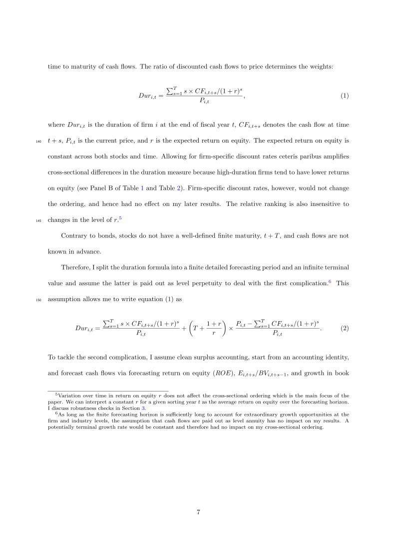
time to maturity of cash flows. The ratio of discounted cash flows to price determines the weights:

Duri,t =

∑Ts=1 s× CFi,t+s/(1 + r)s

Pi,t, (1)

where Duri,t is the duration of firm i at the end of fiscal year t, CFi,t+s denotes the cash flow at time

t+ s, Pi,t is the current price, and r is the expected return on equity. The expected return on equity is140

constant across both stocks and time. Allowing for firm-specific discount rates ceteris paribus amplifies

cross-sectional differences in the duration measure because high-duration firms tend to have lower returns

on equity (see Panel B of Table 1 and Table 2). Firm-specific discount rates, however, would not change

the ordering, and hence had no effect on my later results. The relative ranking is also insensitive to

changes in the level of r.5145

Contrary to bonds, stocks do not have a well-defined finite maturity, t + T , and cash flows are not

known in advance.

Therefore, I split the duration formula into a finite detailed forecasting period and an infinite terminal

value and assume the latter is paid out as level perpetuity to deal with the first complication.6 This

assumption allows me to write equation (1) as150

Duri,t =

∑Ts=1 s× CFi,t+s/(1 + r)s

Pi,t+

(T +

1 + r

r

)×Pi,t −

∑Ts=1 CFi,t+s/(1 + r)s

Pi,t. (2)

To tackle the second complication, I assume clean surplus accounting, start from an accounting identity,

and forecast cash flows via forecasting return on equity (ROE), Ei,t+s/BVi,t+s−1, and growth in book

5Variation over time in return on equity r does not affect the cross-sectional ordering which is the main focus of thepaper. We can interpret a constant r for a given sorting year t as the average return on equity over the forecasting horizon.I discuss robustness checks in Section 3.

6As long as the finite forecasting horizon is sufficiently long to account for extraordinary growth opportunities at thefirm and industry levels, the assumption that cash flows are paid out as level annuity has no impact on my results. Apotentially terminal growth rate would be constant and therefore had no impact on my cross-sectional ordering.

7

equity, (BVi,t+s −BVi,t+s−1)/BVi,t+s−1:

CFi,t+s = Ei,t+s − (BVi,t+s −BVi,t+s−1) (3)

= BVi,t+s−1 ×[

Ei,t+s

BVi,t+s−1− BVi,t+s −BVi,t+s−1

BVi,t+s−1

]. (4)

I model returns on equity and growth in equity as autoregressive processes based on recent findings in

the financial statement analysis literature (see Dechow et al. [27]). I estimate autoregressive parameters

using the pooled CRPS–Compustat universe and assume ROE mean reverts to the average cost of equity

(Nissim and Penman [56]). Nissim and Penman [56] also show that past sales growth is a better predictor

of future growth in book equity than past growth in book equity. I assume that growth in book equity155

mean reverts to the average growth rate of the economy with a coefficient of mean reversion equal to

average historical mean reversion in sales growth.

The book-to-market ratio and cash flow duration are often used interchangeably. A linear relationship

between the book-to-market ratio and duration exists under the assumptions thatROE immediately mean

reverts and that no growth occurs in the book value of equity. I will later show that my measure of cash160

flow duration contains information over and above the book-to-market ratio.

ROE has an AR(1) coefficient of 0.41 and BV of 0.24. I assume a discount rate r of 0.12, a

steady-state average cost of equity of 0.12, an average long-run nominal growth rate of 0.06, and a

detailed forecasting period of 15 years.7 All my findings are robust to reasonable permutations of these

values and to a pre-estimation of these parameters and out-of-sample portfolio sorts (see discussion in165

Section 3).

My sample period is July 1963 until June 2014. The sample is restricted from July 1981 until June

2014, when I make use of the institutional ownership data; July 1982 to June 2009, when I employ

I/B/E/S data on earnings forecasts, realized five year growth, and long term growth forecast; and July

2001 to June 2014, when I employ I/B/E/S forecasts on price targets. To minimize the impact of outliers,170

7Variation in expected inflation could affect the expectations about the long-run nominal growth rate of the economy,but should also affect the nominal discount rate. As stocks are claims on real assets, changes in inflation expectationsshould not affect the value of the firm. Table 5 reports results for five subsamples of ten years each. Return differencesbetween high- and low-duration stocks are similar across different subsamples.

8

I winsorize all variables at the 1% and 99% levels.

2.2. Descriptive Statistics

Table 1 reports summary statistics in Panel A and cross-sectional correlations for various firm

characteristics and return predictors in Panel B. I calculate all statistics annually and then average

over time.175

The average payoff horizon implied by stock prices is about nineteen years. An average standard

deviation of five years hints at substantial cross-sectional heterogeneity in this variable. Institutions hold

about 40% of all shares during my sample period, and the average firm size is $2.1 billion.

Panel B shows that duration is strongly negatively correlated with book-to-market.8 In addition,

high cash flow duration is associated with low payout rates, return-on-equity, and firm age, but high180

growth in sales. No linear association exists between duration and institutional ownership or size. The

institutional ownership ratio is strongly positively correlated with size.

Low-duration stocks tend to be industrial and manufacturing companies, whereas high-duration

stocks were mainly in the software and internet sector in the 1990s and the bio-sciences sector in the

2000s. Table A.1 in the online appendix reports five low- and high-duration firms in 1996 and 2004.185

3. Duration and the Term Structure of Equity Returns

3.1. Portfolios Sorted on Duration

At the end of June each year t from 1963 to 2013, I sort stocks into 10 deciles based on duration for

the fiscal year ending in calendar year t− 1. I rebalance portfolios on an annual basis and weight returns

within portfolio equally.9 Figure 1 plots the time-series average annual portfolio return as a function190

of the average median portfolio duration. This figure exhibits a negative relationship between duration

and holding-period return: low-duration stocks in portfolio 1 have, on average, a one-year holding-period

return of 25%. The high-duration stocks in the last basket, on the contrary, earn less than 10% per

annum.

8Table 12 shows that my findings continue to hold within both value and growth stocks, indicating that duration hasinformation over and above book-to-market.

9The online appendix reports all results for value-weighted returns.

9

I regress excess returns at the portfolio level on various risk factors to test whether traditional risk195

factors can explain the downward-sloping term structure of equity returns,

Ri,t = αi +∑s

βi,sXi,s,t + εi,t, (5)

where Ri,t is excess return of portfolio i at time t, αi is a model-specific pricing error, and βi,s is the

time-series loading of returns on risk factor s, Xi,s, such as size.

Panel A of Table 2 presents monthly mean excess returns, OLS regression coefficients, and pricing

errors for the CAPM with standard errors in parentheses for equally weighted portfolio returns. We200

see in the first line of the table that excess returns monotonically decrease in cash flow duration. In

contrast to the negative relationship for returns, duration is strongly positively related to CAPM betas.

High-duration stocks have a CAPM beta of 1.41 compared to low-duration stocks, which have an exposure

to the market of only 1.05. Decreasing returns and increasing exposure to the market result in a monotonic

negative relationship between duration and pricing errors. A strategy going long low-duration stocks and205

shorting high-duration stocks (D1–D10 in the following) leads to a statistically significant excess return

of 1.29% per month.

Panel B reports monthly Sharpe ratios for the duration-sorted portfolios. The hedge portfolio going

long low-duration stocks and shorting high-duration stocks has a monthly Sharpe ratio of 0.22 which

compares favorably to the monthly Sharpe ratios of the Fama & French five factors, which have monthly210

Sharpe ratios of 0.11 (market), 0.09 (size), 0.13 (value), 0.12 (profitability), and 0.16 (investment) during

my sample period.

Panel C contains results for value-weighted returns. Size and magnitude of return premia

are economically and statistically similar to the equally-weighted returns. The similarity between

equally-weighted and value-weighted returns is expected as size and duration are almost uncorrelated215

(see Table 1).

Panel D shows that delisting returns are not driving my results. If I do not account for delisting

returns, the long-short portfolio return is 1.03% per month compared to the baseline of 1.10% per month.

The CAPM has little explanatory power in the modern sample period (see, e.g., Campbell and

10

Vuolteenaho [16]).10 Table 3 reports alphas for the Fama & French three-factor model, the three-factor220

model augmented with a momentum factor, and the Fama & French five-factor model (Fama and French

[32]). The Fama & French three-factor alpha of the D1–D10 strategy is 0.84% per month, the four-factor

alpha is 0.66% per month, and the five-factor alpha is still a highly statistically significant 0.48% per

month. I report factor loadings in the online appendix to conserve space (see Table A.7 to Table A.9).

Stocks with high cash flow duration tend to have similar loadings on the market, size (SMB), and225

momentum as low-duration stocks, but they have lower loadings on value (HML), profitability (RMW ),

and investment (CMA).

3.2. Sensitivity and Subsample Analysis

The duration measure I present in Section 2 depends on assumptions regarding the persistence in

ROE and sales growth, the long-run growth rate in sales and ROE, the discount rate, and the detailed230

forecasting horizon. Figure 2 reports excess returns of a long-short portfolio for 11 different values of

each parameter. Specifically, the discount rate ranges between 0.07 and 0.17 (baseline 0.12), the detailed

forecast horizon between 10 and 20 years (baseline 15), the sales growth persistence between 0.09 and

0.36 (baseline 0.2411), the ROE persistence between 0.15 and 0.65 (baseline 0.4067), the steady-state

growth rate in sales between 0.01 and 0.11 (baseline 0.06), and the steady-state growth rate in ROE235

between 0.07 and 0.17 (baseline 0.12).

The red line in each panel shows the excess return for the baseline parameter values. We see in the

top panels of Figure 2 that assumptions regarding the discount rate or the detailed forecasting horizon

barely affect the slope of the term structure of equity returns.

In the middle panels, we see moving from a sales growth persistence of 0.09 to a persistence of 0.36240

increases the cross-sectional returns premium from 1.01% to 1.24% per month, whereas increasing the

persistence in ROE lowers the return premium from 1.30% to 0.62%.

In the bottom panels, we see the cross-sectional return premium is most sensitive to extreme

assumptions regarding the long-run sales growth and ROE. Increasing the long-run nominal growth

10One exception is the cross section of stocks sorted on price stickiness (see Weber [68] and Gorodnichenko and Weber[36]). Price stickiness and cash flow duration are uncorrelated in my sample.

11

rate of the economy from a baseline of 6% to 11% cuts the duration premium in half. Decreasing the245

long-run ROE from 12% to 7% instead lowers the excess return by a similar amount.

Table 4 reports excess returns at the portfolio level for economically reasonable variations of

parameter values. Overall, over a wide range of parameter values, we find an economically large and

statistically significant downward-sloping term structure of equity returns. The duration premium seems

a pervasive feature of the data which alleviates concerns of estimation uncertainty driving the results.250

So far, I have used full sample estimates for the autoregressive parameters of the cash flow model.

The evidence so far indicates the downward-sloping term structure of equity returns is a robust feature

of the data and reasonable parameter variations have little impact on the results. To make sure one

can indeed trade on the duration sorts, row (12) of Table 4 reports excess returns for an out-of-sample

exercise. Specifically, I first estimate parameters from 1963 until 1982, use these updated parameters to255

calculate duration at the firm level, and then sort stocks into portfolios from 1983 until the end of my

sample. Also in this out-of-sample exercise, we see a pronounced downward-sloping term structure of

equity returns with low-duration stocks earning an average excess return of 1.21% per month higher than

high-duration stocks.

3.3. Time Variation260

The predictive power of many return characteristics varies over time. Recent examples are the

disappearance of the size premium or the momentum crash (see Daniel and Moskowitz [23] and Freyberger,

Neuhierl, and Weber [34]).

Table 5 reports average monthly excess returns at the portfolio level decade by decade. Across

decades, we see an average monthly duration premium of more than 1% per month. The only exception265

is the very first decade from 1963 to 1973, during which the difference in returns between low- and high-

duration stocks is merely 0.69% per month, which is still economically large and statistically significant.

The term structure of interest rates often inverts during adverse macroeconomic periods. Ait-Sahalia,

Karaman, and Mancini [2] show that the term structure of risk premia is downward-sloping during

recessions, but flat or upward-sloping during normal times. Figure 3 is a time series plot of annual excess270

returns for the low- minus high-duration portfolio (blue line) and the market excess return (red dash-

12

dotted line). Both excess returns show substantial variation over time. During stock market downturns

in the earlier part of the sample up to 2001, we also see in the cross section of equity returns a more

pronounced downward-sloping pattern resulting in a large duration premium. During the recent financial

crisis, instead, low-duration stocks fell more than high-duration stocks, and we observe an upward-sloping275

term structure of equity returns and a negative duration premium. The two time series have a negative

correlation of -29.17%, which increases in absolute value to -36.33% when the sample ends in June 2007.

There is substantial variation over time in the duration premium. Over longer periods, such as

decades, there is a robustly positive downward-sloping term structure of equity returns. The downward

slope was steepest during times of low market returns in the earlier part of the sample, but we observe280

an upward-sloping term structure during the onset of the recent financial crisis. The market return fell

sharply, as did the duration premium.

3.4. Volatility-Managed Duration Portfolios

Moreira and Muir [54] create volatility managed portfolios and show they earn large alphas across

several leading asset pricing models. Specifically, they scale returns by lagged realized variance. The285

strategy takes on less risk when variance was high recently. They find large alphas when they regress the

scaled factor on the original factor or several factors raising the bar for risk-based explanations. Their

results indicate increases in Sharpe ratios relative to the original factor and an expansion of the mean-

variance frontier. Moreira and Muir [54] only focus on scaled factors but did not study the cross-sectional

implications of volatility management.290

Table 6 reports mean returns and alphas relative to several factor models for volatility-managed

duration portfolios.11 We see that volatility managed duration portfolios imply a downward-sloping term

structure of equity returns with a monthly return difference between high- and low-duration portfolios of

1.46% per month, which is even larger than the excess return for unscaled portfolios. When we correct

for exposure to market risk, the long-short excess return increases to 1.58% per month.295

Interestingly, controlling for the three Fama & French factors, the three-factor model augmented

with momentum or the five Fama & French factors has no impact on the return spread at all. Excess

11I thank an anonymous referee for suggesting this analysis.

13

returns are 1.31%, 1.26%, and 1.25%, which stands in contrast to the unscaled duration portfolios in

Table 3.

Moreira and Muir [54] show leading asset pricing models such as the habit formation model of300

Campbell and Cochrane [15], the long run risk model of Bansal and Yaron [9], and the intermediary-based

asset pricing models such as He and Krishnamurthy [40] cannot explain the returns of volatility managed

portfolios, further raising the bar for risk-based explanations to rationalize the downward-sloping term

structure of equity returns.

3.5. Variation with Investor Sentiment305

The results so far show that exposure to traditional risk factors does not suffice to explain the lower

returns of high-duration stocks compared to low-duration stocks. I now investigate a potential mispricing

explanation for this finding. I present Fama & French three-factor adjusted monthly excess returns

following periods of high and low investor sentiment. Stambaugh et al. [62] argue that anomalies should

be stronger following periods of high investor sentiment if mispricing is at the root of the anomaly.12 In310

periods of high investor sentiment, the views of investors about the prospects of many stocks could be

overly optimistic, leading to temporal overpricing. This effect should be strongest for stocks that are

hard to value. A positive return to the D1–D10 strategy should be larger after periods of overpricing and

be mainly attributable to the short leg.13

The mean level of the sentiment index of Baker and Wurgler [7] determines periods of high and low315

investor sentiment. Following Stambaugh et al. [62], I define a high-sentiment month as one in which the

sentiment index was above the mean value in the previous month.

Table 7 presents Fama & French-adjusted excess returns following periods of high and low investor

sentiment in Panel A. The benchmark-adjusted excess returns conditional on high and low sentiment are

the estimates of αH and αL in the following equation:320

Ri,t = αi,HdH,t + αi,LdL,t + βMarketMarkett + βSMBSMBt + βHMLHMLt + εi,t, (6)

12Stambaugh, Yu, and Yuan [63] show that investor sentiment and arbitrage asymmetry can also explain the idiosyncraticvolatility puzzle (see Ang, Hodrick, Xing, and Zhang [5]).

13High-duration firms tend to be younger firms with negative payout ratios and returns on equity, but historically stronggrowth in sales, and are therefore potentially difficult to value (see Table 1).

14

where dH,t and dL,t are dummies indicating high- and low-investor-sentiment months.

A strong negative relationship exists between duration and Fama & French-adjusted excess returns

in high-sentiment months: the D1–D10 strategy earns a highly statistically significant abnormal return

of 1.32% per month. Looking at the numbers for the individual portfolios, we see almost 90% of this

abnormal return is due to the large negative risk-adjusted return for the high-duration portfolio. The325

profitability of the D1–D10 strategy is reduced by a factor of 3 to 0.46% in low-sentiment months.

Comparing the results within portfolios across high- and low-sentiment months indicates high-

duration stocks could be prone to overpricing in periods of high investor sentiment. High-duration

stocks earn negative risk-adjusted returns after periods of high sentiment. No abnormal returns occur in

either direction following periods of low sentiment for high-duration stocks.330

Panel B of Table 7 measures the relationship of changes in the sentiment index and abnormal portfolio

returns. I run separate time-series regressions for each of the 10 portfolios of Fama & French-adjusted

returns on changes in the sentiment index. I find that low- and intermediate-duration portfolios show

no significant relationship, whereas high-duration portfolios load strongly on changes in the sentiment

index. This evidence lends further support to temporary overpricing of high-duration stocks.335

3.6. Analyst Expectations: Earnings Forecasts

Table 8 reports historical cash-flow fundamentals and analyst forecasts.14 Panel A presents the

evolution of the average portfolio long-term earnings growth (LTG) forecast from June of year t until

June of year t + 4. LTG is a forecast of the growth rate in earnings per share before extraordinary

items over the next three to five years. LTG for year t increases monotonically in duration from 13% for340

low-duration stocks to about 26% for portfolio D10. This forecast remains fairly stable for low-duration

stocks as we look at years t+ 1 until t+ 4. On the contrary, for high duration-stocks, LTG falls by 7%

over the next four years.15

The drop in expected long-term growth of high-duration stocks could be due to overly optimistic

14Analysts mainly cover large companies, and therefore the following results might not be representative for the universeof CRPS/Compustat stocks considered so far. In untabulated results, I also find a downward-sloping term structure ofequity returns for the subset of IBES firms.

15I report results for all firms with non-missing LTG forecasts for all periods. Results are unchanged if I look at all firmswith non-missing forecasts at any point in time.

15

initial forecasts or mean reversion in earnings. To discriminate between these two explanations, I report345

realized five-year growth in earnings between years t− 6 to t− 1 and t to t+ 5 in Panel B. For the pre-

portfolio-formation period, we see again a strong positive association between realized five-year growth in

earnings and duration. Low-duration stocks grow on average by 7%, whereas high-duration stocks grow by

31%. This difference in growth rates disappears over the following five years; both high- and low-duration

stocks grow at an annual rate of roughly 10% per annum. This finding hints at an extrapolation bias350

in analyst forecasts for the long-term growth prospects of high-duration firms and further indicates that

market participants are overly optimistic in their perceptions of the prospects of high-duration stocks.

Panel C corroborates this finding looking at three different measures of standardized earnings

surprises following Livnat and Mendenhall [48].16 SUE1 uses a rolling seasonal random walk model

for expected earnings, SUE2 excludes special items, and SUE3 uses IBES-reported analyst forecasts355

and actuals. Stocks with low cash flow duration have a positive median earnings surprise across all

three measures. High-duration stocks, on the other hand, have negative or 0 median earnings surprises.

Research in accounting associates earnings that just meet analyst forecasts with earnings management

(see Skinner and Sloan [61] and Burgstahler and Eames [14]).

3.7. Analyst Expectations: Implied Return Forecasts360

Earnings forecasts and forecasts for long-term growth in earnings are central ingredients for my

duration model in Section 2. My empirical analysis, however, focuses on returns of portfolios sorted on

duration. A direct way to see whether errors in expectations might be at the core of the downward-sloping

term structure of equity returns is to look at return expectations. I follow Asness et al. [6] and create

implied expected returns using analyst target prices. Target prices are an analyst’s forecast for the stock365

price one year into the future.

Panel A of Table 9 reports consensus price targets scaled by book value of equity and price targets

scaled by the current price minus 1, that is, implied return forecasts. Similar to Asness et al. [6] for high-

quality stocks, I find that analysts forecast higher future prices relative to book value for high-duration

stocks. The results for target prices scaled by book value is consistent with the notion that high-duration370

16See also Birru [12]. I thank Justin Birru for suggesting this test.

16

stocks warrant higher prices.

However, analysts’ implied return forecasts do not vary with my measure of cash-flow duration.

Analysts forecast an average expected return of 16% during my sample period for high- and low-duration

stocks. The evidence for price target implied returns is inconsistent with the lower ex-post realized returns

for high-duration stocks, similar to findings in Asness et al. [6].375

Panels B and C study the variation of mean target price implied returns and Fama & French three-

factor alphas of these implied returns with investor sentiment to see whether a systematic expectational

error exists. Greenwood and Shleifer [37] find across six datasets that investors’ return expectations are

positively correlated with past returns and the level of the stock market, but negatively correlated with

model-based expected returns inconsistent with rational expectations. We see both mean returns and380

three-factor alphas are upward-sloping after periods of high investor sentiment, but downward-sloping

after periods of low investor sentiment. The results for analysts’ return forecasts are in stark contrast

to realized returns following periods of high investor sentiment (see Table 7). The evidence adds a

cross-sectional dimension to the market-wide evidence of Greenwood and Shleifer [37] and shows that

expectational errors vary with investor sentiment.385

4. Short-Sale Constraints and the Term Structure of Equity Returns

The previous section illustrates that overpricing could be at the core of a downward-sloping term

structure of equity returns. For overpricing to persist temporarily, however, rational arbitrageurs have

to be restrained from taking sufficiently large short positions to correct the mispricing (see Miller [53]).

In this section, I investigate whether the low returns of high-duration stocks are concentrated among390

short-sale-constrained stocks as proxied by low institutional ownership. I first verbally describe the

testable implications. I then motivate institutional ownership as a proxy for short-sale constraints, and

analyze the interplay of duration and short-sale constraints. I close this section by briefly discussing the

robustness of my results.

4.1. Hypotheses395

Hypothesis 1. The positive abnormal return of going long low-duration stocks and short high-durationstocks (D1–D5 in the following) should be contained in portfolios with low institutionalownership.

17

Hypothesis 1 is a direct implication of the Miller [53] theory. Divergence of opinion about the future

prospects of difficult-to-value, high-duration stocks paired with short-sale constraints leads first to

overpricing and then to low returns once the mispricing is corrected. If the downward-sloping term

structure of equity returns is due to mispricing, the negative relationship between duration and returns400

should become weaker with less binding short-sale constraints.

Hypothesis 2. High-duration portfolios should drive the differences in returns of the D1–D5 strategyacross categories of institutional ownership.

Hypothesis 2 follows from the fact that short-sale constraints allow for overpricing, but not for

underpricing. If a specific stock is underpriced, sophisticated investors can take sufficiently large long

positions independent of short-sale constraints. Furthermore, short-duration stocks pay off most of their405

cash flows in the near-term future, have high returns on equity and low growth in sales, and are therefore

unlikely candidates for overpricing.

4.2. Institutional Ownership and Short-Sale Constraints

Institutional and cultural considerations potentially restrict short-sale activities of institutional

investors. Almazan, Brown, Carlson, and Chapman [3] report that charters restrict about 70% of mutual410

funds to pursue any short-selling activities, and only 2% actually do sell short. Restricted institutions

also do not synthetically engineer short positions. Koski and Pontiff [43] report that only 21% of equity

mutual funds make use of any derivative instruments. Therefore, the only possibility for institutions

to express negative opinions about the outlook of specific stocks is to reduce existing long positions.

Once institutions have sold their positions completely, they have to sit on the sidelines and their negative415

opinions are no longer reflected in market prices. A direct implication of these arguments is that arbitrage

capital increases in institutional ownership.

Contrary to the centralized market for shorting NYSE stocks in the early 20th century, nowadays

short sellers have to search for a stock lender in opaque shorting markets. A lower level of stock loan

supply therefore implies tighter short-sale constraints due to higher search cost (see Duffie, Garleanu, and420

Pedersen [30]). D’Avolio [25] shows that institutional ownership is the most important cross-sectional

determinant of stock loan supply. He also reports that custody banks that engage in stock lending on

behalf of their institutional clients are the most reliable stock lenders, whereas discount brokers are the

18

least dependable.

Short sellers could also have a preference for borrowing stocks from institutional owners. Dechow,425

Hutton, Meulbroek, and Sloan [26] highlight that short squeezes, the recall of stock loans by lenders, are

less likely for stocks with high institutional ownership. In addition, transaction and borrowing costs also

decrease in institutional ownership.

These arguments indicate that short-sale constraints are tighter and the cost of shorting is higher

for stocks with low institutional ownership.430

Institutional ownership is of course an endogenous variable. Institutional ownership has increased

substantially over my sample period which, ceteris paribus, should have increased the stock loan supply

and lowered short-selling costs. ETFs and index funds drove a large part of the increase in institutional

ownership in recent years. My cross-sectional prediction should continue to hold, however, as cash flow

duration and index inclusion are almost orthogonal. These passive institutions also just replicate an index435

and are therefore not actively trading against potential mispricings of stocks.

Stock-lending fees are an alternative measure for short-sale constraints (see Drechsler and Drechsler

[29]). Equity lending data are, however, not available before 2004, as opposed to data on institutional

ownership, which start in 1980 and Markit makes available to researchers only indicative fee data rather

than the actual fee data Drechsler and Drechsler [29] use.440

4.3. Descriptive Statistics

Table 1 illustrates that institutional ownership and size are strongly positively correlated. Many

return anomalies are stronger within smaller stocks, potentially because of lower liquidity and higher

transaction costs (Griffin and Lemmon [38] and Israel and Moskowitz [41]). I follow Nagel [55] to purify

my proxy for short-sale constraints from confounding size effects, and sort on residual institutional445

ownership.17 In each sorting year, I run a cross-sectional regression of logit-transformed institutional

ownership on a constant, the natural logarithm of size, log(ME), as well as log size squared and use the

17Wang [67] and Stambaugh et al. [63], among many other papers, also use residual institutional ownership as a proxyfor short-sale constraints.

19

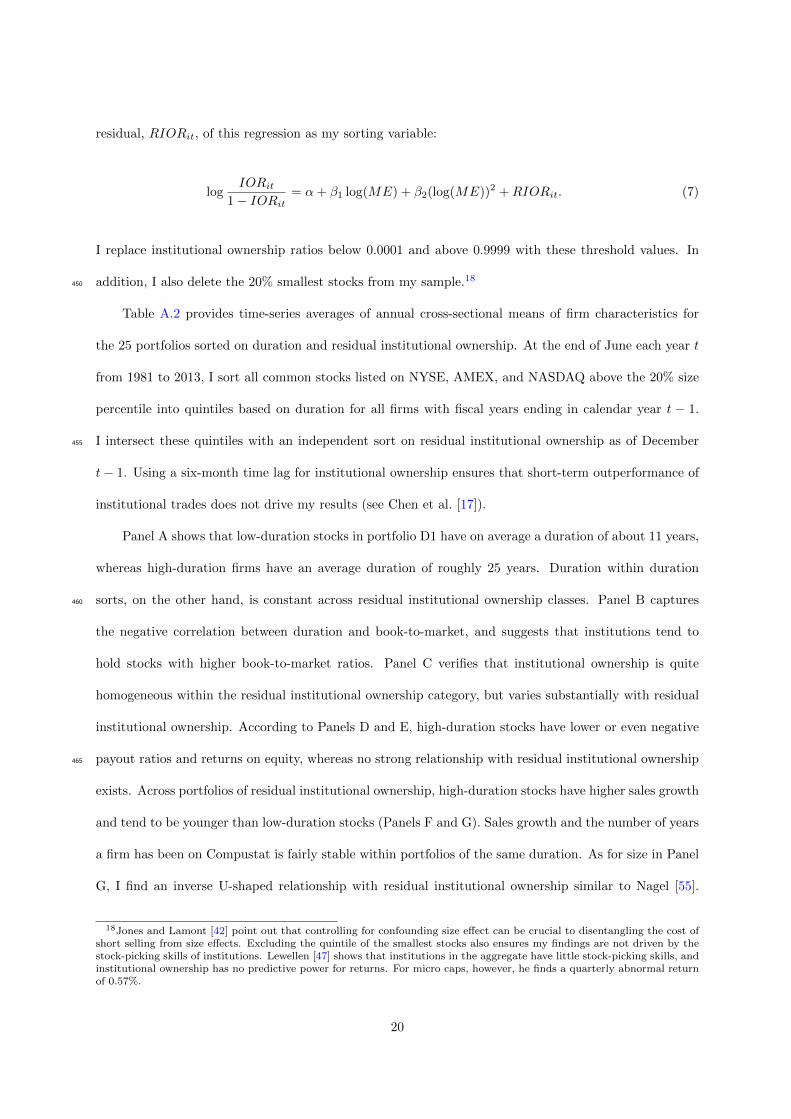
residual, RIORit, of this regression as my sorting variable:

logIORit

1 − IORit= α+ β1 log(ME) + β2(log(ME))2 +RIORit. (7)

I replace institutional ownership ratios below 0.0001 and above 0.9999 with these threshold values. In

addition, I also delete the 20% smallest stocks from my sample.18450

Table A.2 provides time-series averages of annual cross-sectional means of firm characteristics for

the 25 portfolios sorted on duration and residual institutional ownership. At the end of June each year t

from 1981 to 2013, I sort all common stocks listed on NYSE, AMEX, and NASDAQ above the 20% size

percentile into quintiles based on duration for all firms with fiscal years ending in calendar year t − 1.

I intersect these quintiles with an independent sort on residual institutional ownership as of December455

t− 1. Using a six-month time lag for institutional ownership ensures that short-term outperformance of

institutional trades does not drive my results (see Chen et al. [17]).

Panel A shows that low-duration stocks in portfolio D1 have on average a duration of about 11 years,

whereas high-duration firms have an average duration of roughly 25 years. Duration within duration

sorts, on the other hand, is constant across residual institutional ownership classes. Panel B captures460

the negative correlation between duration and book-to-market, and suggests that institutions tend to

hold stocks with higher book-to-market ratios. Panel C verifies that institutional ownership is quite

homogeneous within the residual institutional ownership category, but varies substantially with residual

institutional ownership. According to Panels D and E, high-duration stocks have lower or even negative

payout ratios and returns on equity, whereas no strong relationship with residual institutional ownership465

exists. Across portfolios of residual institutional ownership, high-duration stocks have higher sales growth

and tend to be younger than low-duration stocks (Panels F and G). Sales growth and the number of years

a firm has been on Compustat is fairly stable within portfolios of the same duration. As for size in Panel

G, I find an inverse U-shaped relationship with residual institutional ownership similar to Nagel [55].

18Jones and Lamont [42] point out that controlling for confounding size effect can be crucial to disentangling the cost ofshort selling from size effects. Excluding the quintile of the smallest stocks also ensures my findings are not driven by thestock-picking skills of institutions. Lewellen [47] shows that institutions in the aggregate have little stock-picking skills, andinstitutional ownership has no predictive power for returns. For micro caps, however, he finds a quarterly abnormal returnof 0.57%.

20

However, compared to the variation of size in the CRSP universe, the variation of size across sorts on470

residual ownership is negligible. The sorting on residual ownership is therefore successful in engineering

variation in my short-sale-constraints proxy, independent of size.

Overall, the double sorting generates portfolios that are fairly similar across residual institutional

ownership portfolios, whereas they exhibit large variation across duration categories. High-duration

stocks tend to have characteristics that Baker and Wurgler [7] and Griffin and Lemmon [38] associate475

with speculative, hard-to-value stocks that are prone to divergence of opinion. Daniel et al. [22] draw

on the insights from the psychology literature (see, e.g., Einhorn [31]) and argue mispricing should be

stronger for stocks requiring more judgement in valuing them and for which feedback on this evaluation

is ambiguous in the short run. They mention as an example stocks for which the bulk of cash flows

is expected to be paid out far ahead in the future. In the next subsection, I test whether short-sale480

constraints keep smart money out of the market so that market prices temporarily reflect only the

opinions of the most optimistic investors, leading first to overpricing and then to negative abnormal

returns once this overpricing is corrected.

4.4. Effect of Short-Sale Constraints on the Term Structure of Equity Returns

Table 10 reports monthly mean excess returns for the 25 portfolios. We see a pronounced downward-485

sloping term structure of equity returns for stocks with low residual institutional ownership, which are

potentially the most short sale constrained. Low-duration stocks earn an excess return of 1.02% per

month. The return decreases monotonically in duration. High-duration stocks earn an excess return of

-0.30% per month. The spread in excess returns for the two extreme-duration portfolios is 1.32% per

month and highly statistically significant.19490

Focusing on the long-short portfolio in the last column, we see excess returns decrease monotonically

in residual institutional ownership. For stocks that are potentially the least short-sale constrained,

the long-short portfolio has a statistically insignificant excess return of 0.15% per month, confirming

Hypothesis 1. The difference in returns across residual institutional ownership portfolios of more than

19The results in Table 10 do not directly map into the results of Table 2 as stocks have to be above the 20% size percentileand the sample starts in 1981 rather than 1963.

21

1% per month comes entirely from variation in returns for high-duration stocks. Excess returns increase495

from -0.30% to 0.94% from low to high residual institutional ownership, as predicted by Hypothesis 2.

Low-duration stocks, on the other hand, exhibit no variation with the proxy of short-sale constraints.

Institutional ownership only matters for stocks that are potentially prone to differences in opinion.

A strategy going long the low-residual institutional ownership portfolio and short the high-residual

institutional ownership portfolio (I1 - I5) earns an insignificant excess return of -0.08% for stocks with500

low cash flow duration. This spread decreases monotonically to a highly significant -1.24% per month

for high-duration stocks. This finding is in line with the prediction of the Miller [53] theory. Differences

in opinion paired with short-sale constraints lead to temporal overpricing. High-duration, short-sale

constrained stocks earn low returns once the overpricing is corrected. The data do not back the alternative

hypothesis that institutional ownership reflects smart money. Returns increase in residual institutional505

ownership only for stocks within the highest duration categories.20

Stocks with similar duration but different degrees of residual institutional ownership have similar

fundamentals (see Table A.2). Therefore, it is unlikely that specific investment styles or superior analysis

and information of institutions drive the heterogeneous effect of institutional ownership across duration

categories. Nevertheless, I correct for the portfolios’ exposure to risk in the following to rule out510

covariances with risk factors explain the pattern in excess returns presented in Table 10.21

Correcting for market exposure does not materially change any of the previous findings for excess

returns. Table A.3 in the online appendix shows that the D1–D5 strategy earns a risk-adjusted excess

return of 1.61% per month for stocks with low institutional ownership. This differential decreases to a

statistically insignificant 0.40% for stocks that are potentially the least short sale constrained.515

The CAPM has little explanatory power after 1963. Adjusting for exposure to the three Fama &

French risk factors has no significant impact on pricing errors. We see in Table A.4 in the online appendix

that the abnormal excess returns of the long-short portfolio decrease monotonically in institutional

20Another alternative is that short-sale constraints are also more binding for high-duration stocks. Diether, Lee, andWerner [28], however, show that short-selling activity is higher for growth stocks.

21Lewellen [47] shows that even though institutions as a whole have no stock-picking skills for large stocks, differenttypes of institutions have modest ability compared to the CAPM. Controlling for book-to-market and momentum, however,subsumes this effect.

22

ownership, resulting in a spread across institutional ownership categories of 1.22% per month. This

spread is even slightly larger than the spread in raw or CAPM-adjusted excess returns.22 Adjusting520

as well for momentum reduces pricing errors for high-duration stocks, while having minor impacts for

other categories. The D1–D5 abnormal return is reduced to a highly significant 0.94% per month within

the class of low residual institutional ownership stocks. For the least short-sale-constrained stocks, this

differential abnormal return is -0.10% per month and statistically indistinguishable from zero (see Table

A.5 in the online appendix). Table A.6 in the online appendix reports five-factor alphas. The difference525

in alphas of the long-short portfolios between high- and low-duration stocks is again more than 1% per

month and highly statistically significant.

Tables A.15 to A.19 report the factor loadings for the 25 portfolios. CAPM betas increase from

about 1 for low-duration stocks to about 1.45 for high-duration stocks. This pattern is independent

of institutional ownership. For the Fama & French three-factor model, high-duration stocks have530

higher exposure to market risk and load stronger on size (SMB), but show less common variation with

value (HML). Again, factor loadings are remarkably similar across categories of residual institutional

ownership. High-duration stocks also tend to load more negatively on momentum. The difference in

exposure to market risk and size (SMB) for high- versus low-duration stocks vanishes for the five-factor

model. High-duration stocks tend to load more negatively on value (HML), profitability (RMW ), and535

investment (CWA).

My results are consistent with a mispricing explanation for the negative cross-sectional relationship

between cash flow duration and stock returns in the cross section: the interplay between short-sale

constraints and differences in opinion is what seems responsible for a large part of the empirical regularity

that high-duration stocks earn lower returns compared to low-duration stocks. Exposure to untested risk540

factors might, however, explain the cross section of stocks sorted on cash flow duration. Independent of

my findings, the puzzle of van Binsbergen et al. [64] and van Binsbergen et al. [65] remains: Why do very

short-term assets have such a high risk premium?

22Nevertheless, differences in mean excess returns compared to differences in factor loadings largely drive the effect.

23

4.5. Robustness

I perform several robustness checks to corroborate my previous results and distinguish them from545

findings in the literature. Table 11 contains Fama-French-adjusted pricing errors conditional on size. I

first sort all stocks into two bins based on market capitalization. Within each size bin, I then sort firms

into tertiles based on duration, which I then intersect with an independent sort on residual institutional

ownership. Panel I reports Fama-French alphas for small stocks, whereas Panel II contains alphas for

large stocks. For both small and large stocks, we see a pronounced downward-sloping term structure550

of equity returns for the lowest residual institutional ownership portfolios. The differential in abnormal

returns between high- and low-duration stocks is 1.45% per month for small stocks and 0.72% for large

stocks. This differential abnormal return again decreases in residual institutional ownership, leaving a

highly significant spread of 1.52% between high- and low-residual institutional ownership categories for

small stocks and 0.52% for large stocks.555

Table 12 reports results for a similar exercise with book-to-market as a conditioning variable. The

previous findings hold both for growth stocks in Panel I and value stocks in Panel II. A negative relation

between duration and returns only exists for the most constrained portfolios.

The online appendix also contains all portfolio returns for value-weighted portfolio returns. Results

are similar to the equally weighted returns discussed in the main body of the paper.560

5. Conclusion

I construct a measure of cash flow duration at the firm level using financial statement data. Portfolios

of stocks sorted into deciles based on the measure of cash flow duration exhibit a spread in returns between

low- and high-duration stocks of more than 1% per month. Low-duration stocks have a monthly mean

excess return of 1.45%, whereas high-duration stocks earn 0.32% per month. Exposure to classical risk565

factors cannot explain this pattern in returns. A portfolio long low-duration stocks and short high-

duration stocks earns a statistically significant five-factor alpha of 0.48% per month. The return of this

arbitrage portfolio varies substantially with investor sentiment. It is three times higher after periods of

high investor sentiment.

24

The variation in the return differential with investor sentiment indicates that mispricing could explain570

the downward-sloping term structure of equity returns. I study the earnings expectations of market

participants and find that (a) analysts have overly optimistic growth forecasts in fundamentals for high-

duration stocks, which they adjust downwards over time; (b) analysts extrapolate from past earnings

growth into the future; and (c) high-duration stocks have negative earnings surprises and seem to engage

in earnings management.575

Earnings expectations are central ingredients for my proxy of cash flow duration, but my empirical

analysis focuses on returns of portfolios sorted on duration. I follow Asness et al. [6] and study analysts’

price targets and show that (a) analysts assign higher prices to high-duration stocks and (b) target-price-

implied returns do not vary with cash flow duration, but (c) analysts’ forecasts for expected returns are

upward sloping after periods of high investor sentiment and downward sloping after periods of low investor580

sentiment, in sharp contrast to ex-post realized returns. The evidence adds a cross-sectional dimension to

the market-wide evidence of Greenwood and Shleifer [37] and shows that expectational errors vary with

investor sentiment and could explain parts of the downward-sloping term structure of equity returns.

Mispricing can only persist in the presence of limits to arbitrage. I provide evidence that the interplay

between differences of opinion and short-sale constraints drives my results. Within short-sale-constrained585

stocks, I find a statistically and economically large spread in excess returns between high- and low-duration

stocks of more than 1.32% per month. On the contrary, no difference in returns occurs across duration

categories for unconstrained stocks, consistent with models of rare disaster (Barro [10] and Gabaix [35]).

In line with my proposed explanation for the empirical facts, returns do not vary with short-sale

constraints for short-duration stocks. Any variation in returns is driven by high-duration portfolios, which590

exhibit a spread in excess returns across categories of short-sale constraints of more than 1% per month

without differing in firm characteristics or exposure to risk factors.

Although correcting for standard risk factors has no impact on any of these conclusions, exposure

to other risk factors might still explain the negative relation between cash flow duration and returns.

Variation in the quantity or price of risk is observationally equivalent to variation in investor sentiment.595

My findings complement and extend evidence in van Binsbergen et al. [64] and van Binsbergen,

25

Hueskes, Koijen, and Vrugt [65]. These papers use clean measures of duration, but the dividend strips

and futures data they use limit their analysis to a short sample and assets with duration of only up to

10 years. Using information in the cross section of stock returns, I am able to study a large time series

and assets with duration of more than 25 years.600

26

References

[1] Ai, H., Croce, M., Diercks, A., Li, K., 2012. Production-based term structure of equity returns.Unpublished manuscript, University of Minnesota.

[2] Ait-Sahalia, Y., Karaman, M., Mancini, L., 2015. The term structure of variance swaps and riskpremia. Unpublished manuscript, Princeton University.605

[3] Almazan, A., Brown, K., Carlson, M., Chapman, D., 2004. Why constrain your mutual fundmanager? Journal of Financial Economics 73 (2), 289–321.

[4] Andries, M., Eisenbach, T. M., Schmalz, M. C., 2017. Horizon-dependent risk aversion and thetiming and pricing of uncertainty. Unpublished manuscript, University of Michigan.

[5] Ang, A., Hodrick, R. J., Xing, Y., Zhang, X., 2006. The cross-section of volatility and expected610

returns. The Journal of Finance 61 (1), 259–299.

[6] Asness, C. S., Frazzini, A., Pedersen, L. H., 2014. Quality minus junk. Unpublished manuscript,Copenhagen Business School.

[7] Baker, M., Wurgler, J., 2006. Investor sentiment and the cross-section of stock returns. The Journalof Finance 61 (4), 1645–1680.615

[8] Bansal, R., Dittmar, R. F., Lundblad, C. T., 2005. Consumption, dividends, and the cross sectionof equity returns. The Journal of Finance 60 (4), 1639–1672.

[9] Bansal, R., Yaron, A., 2004. Risks for the long run: A potential resolution of asset pricing puzzles.Journal of Finance 59 (4), 1481–1509.

[10] Barro, R. J., 2006. Rare disasters and asset markets in the twentieth century. The Quarterly Journal620

of Economics 121 (3), 823–866.

[11] Belo, F., Collin-Dufresne, P., Goldstein, R. S., 2015. Dividend dynamics and the term structure ofdividend strips. The Journal of Finance 70 (3), 1115–1160.URL http://dx.doi.org/10.1111/jofi.12242

[12] Birru, J., 2015. Psychological barriers, expectational errors, and underreaction to news. Unpublished625

manuscript, Ohio State University.

[13] Boguth, O., Carlson, M., Fisher, A. J., Simutin, M., 2012. Leverage and the limits of arbitragepricing: Implications for dividend strips and the term structure of equity risk premia. Unpublishedmanuscript, UBC.

[14] Burgstahler, D., Eames, M., 2006. Management of earnings and analysts’ forecasts to achieve zero630

and small positive earnings surprises. Journal of Business Finance & Accounting 33 (5-6), 633–652.URL http://dx.doi.org/10.1111/j.1468-5957.2006.00630.x

[15] Campbell, J., Cochrane, J., 1999. By force of habit: a consumption-based explanation of aggregatestock market behavior. Journal of Political Economy 107 (2), 205–251.

[16] Campbell, J. Y., Vuolteenaho, T., 2004. Bad beta, good beta. The American Economic Review635

94 (5), 1249–1275.URL http://www.aeaweb.org/articles.php?doi=10.1257/0002828043052240

[17] Chen, H.-L., Jegadeesh, N., Wermers, R., 2000. The value of active mutual fund management:An examination of the stockholdings and trades of fund managers. The Journal of Financial andQuantitative Analysis 35 (3), 343–368.640

URL http://www.jstor.org/stable/2676208

[18] Choi, J., Jin, L., Yan, H., 2013. What does stock ownership breadth measure? Review of Finance17 (4), 1239–1278.

[19] Cohen, R. B., Polk, C., Vuolteenaho, T., 2009. The price is (almost) right. The Journal of Finance64 (6), 2739–2782.645

[20] Corhay, A., Kung, H., Schmid, L., 2015. Competition, markups and predictable returns. Unpublishedmanuscript, LBS.

[21] Croce, M., Lettau, M., Ludvigson, S., 2015. Investor information, long-run risk, and the termstructure of equity. The Review of Financial Studies 28 (3), 706–742.

[22] Daniel, K., Hirshleifer, D., Subrahmanyam, A., 1998. Investor psychology and security market under-650

and overreactions. The Journal of Finance 53 (6), 1839–1885.

27

[23] Daniel, K. D., Moskowitz, T. J., 2016. Momentum crashes. Journal of Financial Economics(forthcoming).

[24] Davis, J. L., Fama, E. F., French, K. R., 2000. Characteristics, covariances, and average returns:1929 to 1997. The Journal of Finance 55 (1), 389–406.655

URL http://dx.doi.org/10.1111/0022-1082.00209

[25] D’Avolio, G., 2002. The market for borrowing stock. Journal of Financial Economics 66 (2), 271–306.

[26] Dechow, P., Hutton, A., Meulbroek, L., Sloan, R., 2001. Short-sellers, fundamental analysis, andstock returns. Journal of Financial Economics 61 (1), 77–106.

[27] Dechow, P., Sloan, R., Soliman, M., 2004. Implied equity duration: A new measure of equity risk.660

Review of Accounting Studies 9 (2-3), 197–228.

[28] Diether, K. B., Lee, K.-H., Werner, I. M., 2009. Short-sale strategies and return predictability.Review of Financial Studies 22 (2), 575–607.URL http://rfs.oxfordjournals.org/content/22/2/575.abstract

[29] Drechsler, I., Drechsler, Q. F., 2014. The shorting premium and asset pricing anomalies. Unpublished665

manuscript, New York University.

[30] Duffie, D., Garleanu, N., Pedersen, L., 2002. Securities lending, shorting, and pricing. Journal ofFinancial Economics 66 (2), 307–339.

[31] Einhorn, H., 1980. Overconfidence in judgment. New Directions for Methodology of Social andBehavioral Science 4 (1), 1–16.670

[32] Fama, E. F., French, K. R., 2015. A five-factor asset pricing model. Journal of Financial Economics116 (1), 1–22.

[33] Favilukis, J., Lin, X., 2016. Wage rigidity: A solution to several asset pricing puzzles. The Reviewof Financial Studies 29 (1), 148–192.

[34] Freyberger, J., Neuhierl, A., Weber, M., 2017. Dissecting characteristics non-parametrically.675

Unpublished manuscript, University of Chicago.

[35] Gabaix, X., 2012. Variable rare disasters: An exactly solved framework for ten puzzles in macro-finance. Quarterly Journal of Economics 127 (2), 645–700.

[36] Gorodnichenko, Y., Weber, M., 2016. Are sticky prices costly? Evidence from the stock market.American Economic Review 106 (1), 165–199.680

[37] Greenwood, R., Shleifer, A., 2014. Expectations of returns and expected returns. Review of FinancialStudies 27 (3), 714–746.

[38] Griffin, J. M., Lemmon, M. L., 2002. Book-to-market equity, distress risk, and stock returns. TheJournal of Finance 57 (5), 2317–2336.URL http://dx.doi.org/10.1111/1540-6261.00497685

[39] Hansen, L. P., Heaton, J. C., Li, N., 2008. Consumption strikes back? measuring long-run risk.Journal of Political economy 116 (2), 260–302.

[40] He, Z., Krishnamurthy, A., 2013. Intermediary asset pricing. The American Economic Review 103 (2),732–770.

[41] Israel, R., Moskowitz, T., 2013. The role of shorting, firm size, and time on market anomalies.690

Journal of Financial Economics 108 (2), 275–301.

[42] Jones, C., Lamont, O., 2002. Short-sale constraints and stock returns. Journal of Financial Economics66 (2-3), 207–239.

[43] Koski, J., Pontiff, J., 1999. How are derivatives used? Evidence from the mutual fund industry. TheJournal of Finance 54 (2), 791–816.695

[44] Lettau, M., Ludvigson, S., 2001. Resurrecting the (C) CAPM: a cross-sectional test when risk premiaare time-varying. Journal of Political Economy 109 (6), 1238–1287.

[45] Lettau, M., Maggiori, M., Weber, M., 2014. Conditional risk premia in currency markets and otherasset classes. Journal of Financial Economics 114 (2), 197–225.

[46] Lettau, M., Wachter, J. A., 2007. Why is long-horizon equity less risky? A duration-based700

explanation of the value premium. The Journal of Finance 62 (1), 55–92.

[47] Lewellen, J., 2011. Institutional investors and the limits of arbitrage. Journal of Financial Economics

28

102 (1), 62–80.

[48] Livnat, J., Mendenhall, R. R., 2006. Comparing the post–earnings announcement drift for surprisescalculated from analyst and time series forecasts. Journal of Accounting Research 44 (1), 177–205.705

[49] Lopez, P., Lopez-Salido, D., Vazquez-Grande, F., 2015. Nominal rigidities and the term structuresof equity and bond returns. Tech. rep., Unpublished manuscript, FED Board.

[50] Malloy, C., Moskowitz, T., Vissing-Jørgensen, A., 2009. Long-run stockholder consumption risk andasset returns. The Journal of Finance 64 (6), 2427–2479.

[51] Malloy, C. J., Moskowitz, T. J., VISSING-JØRGENSEN, A., 2009. Long-run stockholder710

consumption risk and asset returns. The Journal of Finance 64 (6), 2427–2479.

[52] Marfe, R., 2016. Income insurance and the equilibrium term-structure of equity. Journal of Finance(forthcoming).

[53] Miller, E. M., 1977. Risk, uncertainty, and divergence of opinion. The Journal of Finance 32 (4),1151–1168.715

URL http://www.jstor.org/stable/2326520

[54] Moreira, A., Muir, T., 2016. Volatility managed portfolios. Journal of Finance (forthcoming).

[55] Nagel, S., 2005. Short sales, institutional investors and the cross-section of stock returns. Journal ofFinancial Economics 78 (2), 277–309.URL http://www.sciencedirect.com/science/article/pii/S0304405X05000735720

[56] Nissim, D., Penman, S., 2001. Ratio analysis and equity valuation: From research to practice. Reviewof Accounting Studies 6 (1), 109–154.

[57] Parker, J., Julliard, C., 2005. Consumption risk and the cross section of expected returns. Journalof Political Economy 113 (1), 185–222.

[58] Santos, T., Veronesi, P., 2010. Habit formation, the cross section of stock returns and the cash-flow725

risk puzzle. Journal of Financial Economics 98 (2), 385–413.

[59] Schulz, F., 2015. On the timing and pricing of dividends: Revisiting the term structure of the equityrisk premium. Tech. rep., Unpublished manuscript, University of Washington.

[60] Shumway, T., 1997. The delisting bias in CRSP data. The Journal of Finance 52 (1), 327–340.URL http://www.jstor.org/stable/2329566730

[61] Skinner, D. J., Sloan, R. G., 2002. Earnings surprises, growth expectations, and stock returns ordon’t let an earnings torpedo sink your portfolio. Review of Accounting Studies 7 (2-3), 289–312.

[62] Stambaugh, R. F., Yu, J., Yuan, Y., 2012. The short of it: Investor sentiment and anomalies. Journalof Financial Economics 104 (2), 288–302.URL http://www.sciencedirect.com/science/article/pii/S0304405X11002649735

[63] Stambaugh, R. F., Yu, J., Yuan, Y., 2015. Arbitrage asymmetry and the idiosyncratic volatilitypuzzle. The Journal of Finance 70 (5), 1903–1948.

[64] van Binsbergen, J., Brandt, M., Koijen, R., 2012. On the timing and pricing of dividends. AmericanEconomic Review 102 (4), 1596–1618.URL http://www.aeaweb.org/articles.php?doi=10.1257/aer.102.4.1596740

[65] van Binsbergen, J., Hueskes, W., Koijen, R., Vrugt, E., 2013. Equity yields. Journal of FinancialEconomics 110 (3), 503–519.

[66] van Binsbergen, J. H., Koijen, R. S., 2015. The term structure of returns: Facts and theory.Unpublished manuscript, Wharton.

[67] Wang, C., 2014. Institutional holding, low beta and idiosyncratic volatility anomalies. Unpublished745

manuscript, Yale SOM.

[68] Weber, M., 2015. Nominal rigidities and asset pricing. Unpublished manuscript, University ofChicago.

29

Figure 1: Average Term Structure of Equity

6 9 12 15 18 21 24

10

12

14

16

18

20

22

24

AnnualReturn

[%]

Duration [years]

This figure plots the time series average annual portfolio return as a function of the average median portfolio cash flow

duration. I sort all common stocks listed on NYSE, AMEX, and NASDAQ at the end of June each year t from 1963

to 2013 into deciles based on duration for all firms with fiscal years ending in year t-1. I weight returns equally and

include delisting returns. If a firm is delisted for cause (delisting code between 400 and 591) and has missing delisting

return, I assume a delisting return of -30% following Shumway [60]. Financial statement data come from Compustat.

For missing Compustat book equity values, I use the Moody’s book equity information collected by Davis et al. [24].

30

Figure 2: Sensitivity Analysis

0.08 0.10 0.12 0.14 0.16

0.50

0.90

1.30

baseline

Discount Rate

11 13 15 17 19

Forcast Horizon [years]

baseline

0.12 0.18 0.24 0.30 0.36

0.50

0.90

1.30

Monthly

Return

[%]

Sales Growth Persistence

baseline

0.20 0.30 0.40 0.50 0.60

ROE Persistence

baseline

0.02 0.04 0.06 0.08 0.10

0.50

0.90

1.30

Steady State Sales Growth

baseline

0.08 0.10 0.12 0.14 0.16

Steady State ROE

baseline

This figure plots monthly long-short excess returns for variations in the parameter values I use to construct cash flow

duration at the firm level (see equation (2)). I sort all common stocks listed on NYSE, AMEX, and NASDAQ at the end

of June each year t from 1963 to 2013 into deciles based on duration for all firms with fiscal years ending in year t-1. I

weight returns equally and include delisting returns. If a firm is delisted for cause (delisting code between 400 and 591)

and has missing delisting return, I assume a delisting return of -30% following Shumway [60]. Financial statement

data come from Compustat. For missing Compustat book equity values, I use the Moody’s book equity information

collected by Davis et al. [24].

31

Figure 3: Time Series of Returns

−40

−20

0

20

40

60

80

100

1964

1969

1974

1979

1984

1989

1994

1999

2004

2009

2014

Year

ρDur,M = −29.17%

AnnualReturn

[%]

DurationMarket

This figure plots annual long-short excess returns based on 10 cash flow duration sorted portfolios (blue line) and the

market excess return (red dash-dotted line). I sort all common stocks listed on NYSE, AMEX, and NASDAQ at the end

of June each year t from 1963 to 2013 into deciles based on duration for all firms with fiscal years ending in year t-1. I

weight returns equally and include delisting returns. If a firm is delisted for cause (delisting code between 400 and 591)

and has missing delisting return, I assume a delisting return of -30% following Shumway [60]. Financial statement

data come from Compustat. For missing Compustat book equity values, I use the Moody’s book equity information

collected by Davis et al. [24].

32

Table 1: Summary Statistics and Correlations for Firm Characteristics and Return Predictors

This table reports time series averages of annual cross-sectional means and standard

deviations for firm characteristics and return predictors in Panel A and contemporaneous

correlations of these variables in Panel B. Dur is cash-flow duration; BM is the

book-to-market ratio; IOR is the fraction of shares institutions hold; PR is net payout over

net income; ROE is return on equity; Sales g is sales growth; ME is the market capitalization

in millions; and Age is the number of years a firm has been on Compustat. Institutional

ownership information is obtained from the Thomson Reuters 13F database. Financial

statement data come from Compustat. For missing Compustat book equity values, I use

the Moody’s book equity information collected by Davis et al. [24]. The sample period is

June 1981 to June 2014. I only use stocks above the 20th size percentile.

Dur BM IOR PR ROE Sales g ME Age

Panel A. Means and Standard Deviations

Mean 18.77 0.67 0.44 -0.01 0.05 0.22 2125 17.59

Std 5.37 0.53 0.23 2.10 0.54 0.59 6197 11.46

Panel B. Contemporaneous Correlations

Dur -0.70 -0.08 -0.10 -0.39 0.34 0.04 -0.19

B/M -0.01 0.08 -0.04 -0.16 -0.11 0.11

IOR 0.06 0.18 -0.10 0.22 0.26

PR -0.05 -0.24 0.08 0.20

ROE -0.02 0.10 0.09

Sale g -0.04 -0.20

ME 0.30

33

Tab

le2:M

ean

Excess

Retu

rnsof10

Portfoliosso

rte

don

Duration

Pa

nel

Are

port

sm

on

thly

mea

nex

cess

retu

rns,

tim

ese

ries

fact

or

loa

din

gs(β

),a

nd

pri

cin

ger

rors

(α)

for

the

CA

PM

for

ten

port

foli

os

sort

edo

n

du

rati

on

(Du

r)w

ith

OL

Sst

an

da

rder

rors

inpa

ren

thes

esin

Pa

nel

A.

Iso

rta

llco

mm

on

stoc

ksli

sted

on

NY

SE

,A

ME

X,

an

dN

AS

DA

Qa

tth

een

d

of

Ju

ne

each

yea

rt

fro

m1

96

3to

20

13

into

dec

iles

base

do

nd

ura

tio

nfo

ra

llfi

rms

wit

hfi

sca

lyea

rsen

din

gin

yea

rt-

1.

Iw

eigh

tre

turn

seq

ua

lly

an

din

clu

de

del

isti

ng

retu

rns.

Ifa

firm

isd

elis

ted

for

cau

se(d

elis

tin

gco

de

betw

een

40

0a

nd

59

1)

an

dh

as

am

issi

ng

del

isti

ng

retu

rn,

Ia

ssu

me

a

del

isti

ng

retu

rno

f-3

0%

foll

ow

ing

Sh

um

wa

y[6

0].

Ma

rket

isth

eva

lue

wei

ghte

dre

turn

on

all

NY

SE

,A

ME

X,

an

dN

AS

DA

Qco

mm

on

stoc

ksm

inu

sth

e

on

e-m

on

thT

rea

sury

bill

rate

.F

ina

nci

al

sta

tem

ent

da

taco

me

fro

mC

om

pu

sta

t.F

or

mis

sin

gC

om

pu

sta

tbo

ok

equ

ity

valu

es,

Iu

seth

eM

ood

y’s

boo

k

equ

ity

info

rma

tio

nco

llec

ted

byD

avi

set

al.

[24

].P

an

elB

repo

rts

mo

nth

lyS

ha

rpe

Ra

tio

s,P

an

elC

repo

rts

resu

lts

for

valu

e-w

eigh

ted

port

foli

ore

turn

s,

an

dP

an

elD

for

equ

all

y-w

eigh

ted

port

foli

ore

turn

sw

ith

ou

tin

clu

din

gd

elis

tin

gre

turn

s.

Low

Du

rD

2D

3D

4D

5D

6D

7D

8D

9H

igh

Du

rD

1–D

10

PanelA.M

ean-E

xcess

Retu

rnsand

CAPM

Mea

n1.

431.

241.1

41.0

41.0

00.9

70.8

10.6

80.6

20.3

21.1

0

SE

(0.2

5)(0

.24)

(0.2

4)

(0.2

3)

(0.2

4)

(0.2

4)

(0.2

5)

(0.2

6)

(0.3

0)

(0.3

5)

(0.2

0)

βCAPM

1.05

1.06

1.0

81.1

01.1

31.1

51.1

91.2

61.3

91.4

1-0

.36

SE

(0.0

4)(0

.03)

(0.0

3)

(0.0

3)

(0.0

3)

(0.0

3)

(0.0

3)

(0.0

3)

(0.0

4)

(0.0

5)

(0.0

4)

αCAPM

0.90

0.71

0.6

00.4

90.4

30.3

90.2

10.0

5-0

.08

-0.3

91.2

9

SE

(0.1

7)(0

.14)

(0.1

3)

(0.1

2)

(0.1

2)

(0.1

2)

(0.1

2)

(0.1

3)

(0.1

7)

(0.2

4)

(0.1

9)

PanelB.M

onth

lySharp

eRatios

Sh

arp

eR

atio

0.23

0.21

0.2

00.1

80.1

70.1

60.1

30.1

10.0

80.0

40.2

2

PanelC.Value-w

eighted

Retu

rns

Mea

n1.

040.

870.8

80.8

30.7

40.6

20.5

50.5

50.4

3-0

.04

1.0

8

SE

(0.2

4)(0

.22)

(0.2

1)

(0.2

0)

(0.1

9)

(0.1

9)

(0.1

9)

(0.1

9)

(0.2

2)

(0.3

1)

(0.2

4)

PanelD.NoDelistingRetu

rns

Mea

n1.

491.

271.1

71.0

71.0

20.9

80.8

30.7

00.6

70.4

71.0

3

SE

(0.2

5)(0

.24)

(0.2

4)

(0.2

4)

(0.2

4)

(0.2

4)

(0.2

5)

(0.2

6)

(0.3

0)

(0.3

5)

(0.2

0)

34

Tab

le3:Fam

a&

French

Facto

rAlp

hasof10

Portfoliosso

rte

don

Duration

Th

ista

ble

repo

rts

pri

cin

ger

rors

(α)

for

the

Fa

ma

&F

ren

chth

ree-

fact

or

mod

el(α

F&F3),

the

thre

e-fa

cto

rm

odel

au

gmen

ted

wit

hm

om

entu

m

(αF&F4),

an

dth

eF

am

a&

Fre

nch

five

-fa

cto

rm

odel

(αF&F5)

for

ten

port

foli

os

sort

edo

nd

ura

tio

n(D

ur)

wit

hO

LS

sta

nd

ard

erro

rsin

pare

nth

eses

.

Iso

rta

llco

mm

on

stoc

ksli

sted

on

NY

SE

,A

ME

X,

an

dN

AS

DA

Qa

tth

een

do

fJ

un

eea

chyea

rt

fro

m1

96

3to

20

13

into

dec

iles

base

do

nd

ura

tio

n

for

all

firm

sw

ith

fisc

al

yea

rsen

din

gin

yea

rt-

1.

Iw

eigh

tre

turn

seq

ua

lly

an

din

clu

de

del

isti

ng

retu

rns.

Ifa

firm

isd

elis

ted

for

cau

se(d

elis

tin

g

cod

ebe

twee

n4

00

an

d5

91

)a

nd

ha

sa

mis

sin

gd

elis

tin

gre

turn

,I

ass

um

ea

del

isti

ng

retu

rno

f-3

0%

foll

ow

ing

Sh

um

wa

y[6

0].

Ma

rket

isth

e

valu

e-w

eigh

ted

retu

rno

na

llN

YS

E,

AM

EX

,a

nd

NA

SD

AQ

com

mo

nst

ocks

min

us

the

on

e-m

on

thT

rea

sury

bill

rate

,SMB

isth

ea

vera

gere

turn

on

thre

esm

all

port

foli

os

min

us

the

ave

rage

retu

rno

nth

ree

big

port

foli

os,HML

isth

ea

vera

gere

turn

on

two

valu

epo

rtfo

lio

sm

inu

sth

ea

vera

ge

retu

rno

ntw

ogr

ow

thpo

rtfo

lio

s,Mom

isth

ea

vera

gere

turn

on

two

hig

hp

rio

rre

turn

port

foli

os

min

us

the

ave

rage

retu

rno

ntw

olo

wp

rio

rre

turn

port

foli

os,RMW

isth

ea

vera

gere

turn

on

two

robu

sto

pera

tin

gp

rofi

tabi

lity

port

foli

os

min

us

the

ave

rage

retu

rno

ntw

ow

eak

ope

rati

ng

pro

fita

bili

ty

port

foli

os,

an

dCMA

isth

ea

vera

gere

turn

on

two

con

serv

ati

vein

vest

men

tpo

rtfo

lio

sm

inu

sth

ea

vera

gere

turn

on

two

agg

ress

ive

inve

stm

ent

port

foli

os.

Fin

an

cia

lst

ate

men

td

ata

com

efr

om

Co

mp

ust

at.

Fo

rm

issi

ng

Co

mp

ust

at

boo

keq

uit

yva

lues

,I

use

the

Moo

dy’s

boo

keq

uit

yin

form

ati

on

coll

ecte

dby

Da

vis

eta

l.[2

4].

Low

Du

rD

2D

3D

4D

5D

6D

7D

8D

9H

igh

Du

rD

1–D

10

αF&F3

0.46

0.34

0.26

0.1

80.1

70.1

50.0

3-0

.03

-0.0

8-0

.38

0.8

4

SE

(0.1

0)(0

.08)

(0.0

7)

(0.0

6)

(0.0

6)

(0.0

6)

(0.0

7)

(0.0

7)

(0.1

1)

(0.1

9)

(0.1

5)

αF&F4

0.60

0.48

0.38

0.3

10.3

00.3

20.2

00.1

60.1

8-0

.07

0.6

6

SE

(0.1

0)(0

.07)

(0.0

6)

(0.0

6)

(0.0

6)

(0.0

6)

(0.0

6)

(0.0

6)

(0.1

0)

(0.1

8)

(0.1

5)

αF&F5

0.49

0.35

0.26

0.1

70.1

70.1

60.0

70.0

70.1

40.0

10.4

8

SE

(0.1

0)(0

.08)

(0.0

7)

(0.0

6)

(0.0

6)

(0.0

7)

(0.0

7)

(0.0

7)

(0.1

0)

(0.1

7)

(0.1

4)

35

Tab

le4:M

ean

Excess

Retu

rnsof10

Portfoliosso

rte

don

Duration

(robustness)

Th

ista

ble

repo

rts

mo

nth

lym

ean

exce

ssre

turn

sw

ith

OL

Sst

an

da

rder

rors

inpa

ren

thes

esfo

rva

ria

tio

ns

of

the

para

met

erva

lues

use

dto

calc

ula

te

du

rati

on

inS

ecti

on

2.

Iso

rta

llco

mm

on

stoc

ksli

sted

on

NY

SE

,A

ME

X,

an

dN

AS

DA

Qa

tth

een

do

fJ

un

eea

chyea

rt

fro

m1

96

3to

20

13

into

dec

iles

base

do

nd

ura

tio

nfo

ra

llfi

rms

wit

hfi

sca

lyea

rsen

din

gin

yea

rt-

1.

Iw

eigh

tre

turn

seq

ua

lly

an

din

clu

de

del

isti

ng

retu

rns.

Ifa

firm

isd

elis

ted

for

cau

se(d

elis

tin

gco

de

betw

een

40

0a

nd

59

1)

an

dh

as

am

issi

ng

del

isti

ng

retu

rn,

Ia

ssu

me

ad

elis

tin

gre

turn

of

-30

%fo

llo

win

gS

hu

mw

ay

[60

].F

ina

nci

al

sta

tem

ent

da

taco

me

fro

mC

om

pu

sta

t.F

or

mis

sin

gC

om

pu

sta

tbo

ok

equ

ity

valu

es,

Iu

seth

eM

ood

y’s

boo

keq

uit

yin

form

ati

on

coll

ecte

dby

Da

vis

eta

l.

[24

].

Low

Du

rD

2D

3D

4D

5D

6D

7D

8D

9H

igh

Du

rD

1–D

10

(1)

r=

0.10

1.45

1.23

1.1

31.0

61.0

00.9

50.8

10.6

80.6

60.2

81.1

7

(0.2

5)(0

.24)

(0.2

4)

(0.2

4)

(0.2

4)

(0.2

4)

(0.2

5)

(0.2

6)

(0.3

0)

(0.3

5)

(0.2

0)

(2)

r=

0.14

1.42

1.24

1.1

31.0

31.0

40.9

40.8

40.6

40.6

50.3

31.1

0

(0.2

5)(0

.24)

(0.2

3)

(0.2

4)

(0.2

3)

(0.2

4)

(0.2

4)

(0.2

6)

(0.3

1)

(0.3

5)

(0.2

0)

(3)

ar r

oe

=0.

301.

481.

211.1

31.1

20.9

80.9

70.8

00.7

30.5

60.2

51.2

3

(0.2

6)(0

.24)

(0.2

4)

(0.2

4)

(0.2

4)

(0.2

4)

(0.2

5)

(0.2

6)

(0.2

9)

(0.3

5)

(0.2

0)

(4)

ar r

oe

=0.

501.

341.

301.1

01.0

60.9

70.9

50.8

20.6

50.6

60.4

20.9

3

(0.2

5)(0

.23)

(0.2

3)

(0.2

4)

(0.2

3)

(0.2

4)

(0.2

5)

(0.2

6)

(0.3

1)

(0.3

6)

(0.2

0)

(6)

roe s

s=

0.10

1.40

1.27

1.1

21.0

41.0

10.9

60.8

10.6

70.6

10.3

61.0

4

(0.2

5)(0

.24)

(0.2

3)

(0.2

4)

(0.2

3)

(0.2

4)

(0.2

5)

(0.2

6)

(0.3

1)

(0.3

5)

(0.2

0)

(5)

roe s

s=

0.14

1.45

1.24

1.1

11.0

80.9

90.9

50.8

20.7

00.6

50.2

61.1

8

(0.2

5)(0

.24)

(0.2

4)

(0.2

4)

(0.2

4)

(0.2

4)

(0.2

5)

(0.2

6)

(0.2

9)

(0.3

5)

(0.2

0)

(9)

ar s

g=

0.20

1.42

1.25

1.1

41.0

21.0

10.9

50.8

00.7

00.6

30.3

31.0

9

(0.2

5)(0

.24)

(0.2

4)

(0.2

3)

(0.2

4)

(0.2

4)

(0.2

5)

(0.2

6)

(0.3

0)

(0.3

5)

(0.2

0)

(10)

ar s

g=

0.30

1.45

1.22

1.1

31.0

71.0

30.9

70.8

10.6

70.5

90.3

01.1

5

(0.2

5)(0

.24)

(0.2

3)

(0.2

3)

(0.2

4)

(0.2

4)

(0.2

5)

(0.2

6)

(0.3

0)

(0.3

5)

(0.2

0)

(7)

sgss

=0.

081.

441.

231.1

31.0

70.9

80.9

60.8

10.7

10.6

40.2

61.1

8

(0.2

5)(0

.24)

(0.2

4)

(0.2

4)

(0.2

4)

(0.2

4)

(0.2

5)

(0.2

6)

(0.2

9)

(0.3

5)

(0.2

0)

(8)

sgss

=0.

041.

401.

251.1

51.0

40.9

70.9

60.8

20.6

70.6

20.3

91.0

1

(0.2

5)(0

.24)

(0.2

3)

(0.2

4)

(0.2

3)

(0.2

4)

(0.2

5)

(0.2

6)

(0.3

1)

(0.3

5)

(0.2

0)

(11)

horizon

=10

1.39

1.26

1.1

21.0

70.9

60.9

40.8

30.6

70.6

00.4

10.9

8

(0.2

5)(0

.24)

(0.2

3)

(0.2

4)

(0.2

3)

(0.2

4)

(0.2

4)

(0.2

7)

(0.3

1)

(0.3

5)

(0.2

0)

(12)

pre

-est

imat

ion

1.36

1.18

1.0

50.9

80.9

60.9

00.7

40.6

10.5

90.1

41.2

1

(0.3

1)(0

.29)

(0.2

9)

(0.2

9)

(0.2

9)

(0.3

0)

(0.3

0)

(0.3

3)

(0.4

0)

(0.4

9)

(0.2

9)

36

Tab

le5:M

ean

Excess

Retu

rnsof10

Portfoliosso

rte

don

Duration

(subsa

mples)

Th

ista

ble

repo

rts

mo

nth

lym

ean

exce

ssre

turn

sw

ith

OL

Sst

an

da

rder

rors

inpa

ren

thes

esfo

rd

iffer

ent

subs

am

ple

s.I

sort

all

com

mo

nst

ocks

list

edo

n

NY

SE

,A

ME

X,

an

dN

AS

DA

Qa

tth

een

do

fJ

un

eea

chyea

rt

fro

m1

96

3to

20

13

into

dec

iles

base

do

nd

ura

tio

nfo

ra

llfi

rms

wit

hfi

sca

lyea

rsen

din

g

inyea

rt-

1.

Iw

eigh

tre

turn

seq

ua

lly

an

din

clu

de

del

isti

ng

retu

rns.

Ifa

firm

isd

elis

ted

for

cau

se(d

elis

tin

gco

de

betw

een

40

0a

nd

59

1)

an

dh

as

a

mis

sin

gd

elis

tin

gre

turn

,I

ass

um

ea

del

isti

ng

retu

rno

f-3

0%

foll

ow

ing

Sh

um

wa

y[6

0].

Fin

an

cia

lst

ate

men

td

ata

com

efr

om

Co

mp

ust

at.

Fo

rm

issi

ng

Co

mp

ust

at

boo

keq

uit

yva

lues

,I

use

the

Moo

dy’s

boo

keq

uit

yin

form

ati

on

coll

ecte

dby

Da

vis

eta

l.[2

4].

Low

Du

rD

2D

3D

4D

5D

6D

7D

8D

9H

igh

Du

rD

1–D

10

PanelA.July

1963–June1973

Mea

n0.

910.

820.

73

0.7

30.5

10.4

30.2

90.1

50.1

20.2

30.6

9

SE

(0.5

3)(0

.51)

(0.5

1)

(0.5

2)

(0.5

0)

(0.5

1)

(0.5

2)

(0.5

3)

(0.5

6)

(0.5

7)

(0.2

5)

PanelB.July

1973–June1983

Mea

n2.

171.

871.

78

1.6

61.6

31.7

01.5

41.4

01.3

50.8

31.3

4

SE

(0.6

7)(0

.63)

(0.6

1)

(0.6

1)

(0.6

1)

(0.6

3)

(0.6

4)

(0.6

6)

(0.6

9)

(0.7

4)

(0.3

9)

PanelC.July

1983–June1993

Mea

n0.

960.

790.

66

0.4

90.5

80.4

40.1

80.0

6-0

.11

-0.4

11.3

7

SE

(0.4

6)(0

.45)

(0.4

7)

(0.4

8)

(0.4

9)

(0.5

0)

(0.5

0)

(0.5

1)

(0.5

7)

(0.6

8)

(0.3

5)

PanelD.July

1993–June2003

Mea

n1.

381.

271.

15

0.9

81.0

80.9

80.9

00.8

30.7

40.2

81.1

0

SE

(0.4

9)(0

.48)

(0.5

0)

(0.4

7)

(0.5

2)

(0.5

3)

(0.5

8)

(0.6

8)

(0.9

1)

(1.1

2)

(0.7

6)

PanelE.July

2003–June2014

Mea

n1.

681.

441.

37

1.3

31.1

91.2

61.0

90.9

40.9

50.6

41.0

4

SE

(0.6

1)(0

.56)

(0.5

3)

(0.5

2)

(0.5

0)

(0.5

0)

(0.5

0)

(0.5

0)

(0.5

6)

(0.6

9)

(0.3

4)

37

Tab

le6:M

ean

Retu

rnsand

Alp

hasof10

Portfoliosso

rte

don

Duration:Volatility

-managed

Portfolios

Th

ista

ble

repo

rts

mea

nre

turn

sa

nd

pri

cin

ger

rors

(α)

for

the

CA

PM

(αCAPM

),th

eF

am

a&

Fre

nch

thre

e-fa

cto

rm

odel

(αF&F3),

the

thre

e-fa

cto

r

mod

ela

ugm

ente

dw

ith

mo

men

tum

(αF&F4),

an

dth

eF

am

a&

Fre

nch

five

-fa

cto

rm

odel

(αF&F5)

for

ten

port

foli

os

sort

edo

nd

ura

tio

n(D

ur)

wit

h

OL

Sst

an

da

rder

rors

inpa

ren

thes

es.

Po

rtfo

lio

retu

rns

are

sca

led

byth

ep

revi

ou

sm

on

ths

rea

lize

dva

ria

nce

as

inM

ore

ira

an

dM

uir

[54

].I

sort

all

com

mo

nst

ocks

list

edo

nN

YS

E,

AM

EX

,a

nd

NA

SD

AQ

at

the

end

of

Ju

ne

each

yea

rt

fro

m1

96

3to

20

13

into

dec

iles

base

do

nd

ura

tio

nfo

r

all

firm

sw

ith

fisc

al

yea

rsen

din

gin

yea

rt-

1.

Iw

eigh

tre

turn

seq

ua

lly

an

din

clu

de

del

isti

ng

retu

rns.

Ifa

firm

isd

elis

ted

for

cau

se(d

elis

tin

g

cod

ebe

twee

n4

00

an

d5

91

)a

nd

ha

sa

mis

sin

gd

elis

tin

gre

turn

,I

ass

um

ea

del

isti

ng

retu

rno

f-3

0%

foll

ow

ing

Sh

um

wa

y[6

0].

Ma

rket

isth

e

valu

e-w

eigh

ted

retu

rno

na

llN

YS

E,

AM

EX

,a

nd

NA

SD

AQ

com

mo

nst

ocks

min

us

the

on

e-m

on

thT

rea

sury

bill

rate

,SMB

isth

ea

vera

gere

turn

on

thre

esm

all

port

foli

os

min

us

the

ave

rage

retu

rno

nth

ree

big

port

foli

os,HML

isth

ea

vera

gere

turn

on

two

valu

epo

rtfo

lio

sm

inu

sth

ea

vera

ge

retu

rno

ntw

ogr

ow

thpo

rtfo

lio

s,Mom

isth

ea

vera

gere

turn

on

two

hig

hp

rio

rre

turn

port

foli

os

min

us

the

ave

rage

retu

rno

ntw

olo

wp

rio

rre

turn

port

foli

os,RMW

isth

ea

vera

gere

turn

on

two

robu

sto

pera

tin

gp

rofi

tabi

lity

port

foli

os

min

us

the

ave

rage

retu

rno

ntw

ow

eak

ope

rati

ng

pro

fita

bili

ty

port

foli

os,

an

dCMA

isth

ea

vera

gere

turn

on

two

con

serv

ati

vein

vest

men

tpo

rtfo

lio

sm

inu

sth

ea

vera

gere

turn

on

two

agg

ress

ive

inve

stm

ent

port

foli

os.

Fin

an

cia

lst

ate

men

td

ata

com

efr

om

Co

mp

ust

at.

Fo

rm

issi

ng

Co

mp

ust

at

boo

keq

uit

yva

lues

,I

use

the

Moo

dy’s

boo

keq

uit

yin

form

ati

on

coll

ecte

dby

Da

vis

eta

l.[2

4].

Low

Du

rD

2D

3D

4D

5D

6D

7D

8D

9H

igh

Du

rD

1–D

10

Mea

n1.

991.

681.

60

1.5

01.5

31.4

41.2

81.1

31.1

50.9

91.4

6

SE

(0.2

5)(0

.24)

(0.2

4)

(0.2

3)

(0.2

4)

(0.2

4)

(0.2

5)

(0.2

6)

(0.3

0)

(0.3

5)

(0.2

0)

αCAPM

1.58

1.29

1.20

1.1

21.1

11.0

20.8

70.6

70.6

50.4

41.5

8

SE

(0.2

0)(0

.19)

(0.1

9)

(0.1

9)

(0.1

8)

(0.1

9)

(0.2

0)

(0.2

0)

(0.2

4)

(0.2

9)

(0.2

0)

αF&F3

1.36

1.12

1.02

0.9

80.9

90.9

00.7

60.6

10.5

50.3

41.3

1

SE

(0.1

9)(0

.18)

(0.1

8)

(0.1

8)

(0.1

8)

(0.1

8)

(0.1

9)

(0.1

9)

(0.2

3)

(0.2

7)

(0.1

9)

αF&F4

1.26

1.03

0.92

0.8

70.8

50.7

90.6

20.4

60.4

00.1

91.2

6

SE

(0.1

9)(0

.19)

(0.1

8)

(0.1

9)

(0.1

8)

(0.1

8)

(0.1

9)

(0.1

9)

(0.2

3)

(0.2

7)

(0.1

9)

αF&F5

1.20

0.95

0.87

0.8

40.8

50.7

60.6

10.4

40.3

70.2

01.2

5

SE

(0.1

9)(0

.19)

(0.1

8)

(0.1

9)

(0.1

8)

(0.1

8)

(0.1

9)

(0.1

9)

(0.2

3)

(0.2

8)

(0.1

9)

38

Tab

le7:Fam

a&

French

Alp

hasof10

Portfoliosso

rte

don

Duration

Conditionalon

InvestorSentim

ent

Th

ista

ble

repo

rts

ben

chm

ark

-ad

just

edm

ean

exce

ssre

turn

sfo

llo

win

gpe

riod

so

fh

igh

an

dlo

win

vest

or

sen

tim

ent

inP

an

elA

,a

sw

ell

as

sen

tim

ent

beta

s

inP

an

elB

for

ten

port

foli

os

sort

edo

nd

ura

tio

n(D

ur)

wit

hO

LS

sta

nd

ard

erro

rsin

pare

nth

eses

.I

sort

all

com

mo

nst

ocks

list

edo

nN

YS

E,

AM

EX

,a

nd

NA

SD

AQ

at

the

end

of

Ju

ne

each

yea

rt

fro

m1

96

3to

20

13

into

dec

iles

base

do

nd

ura

tio

nfo

ra

llfi

rms

wit

hfi

sca

lyea

rsen

din

gin

yea

rt-

1.

Iw

eigh

t

retu

rns

equ

all

ya

nd

incl

ud

ed

elis

tin

gre

turn

s.If

afi

rmis

del

iste

dfo

rca

use

(del

isti

ng

cod

ebe

twee

n4

00

an

d5

91

)a

nd

ha

sa

mis

sin

gd

elis

tin

gre

turn

,I

ass

um

ea

del

isti

ng

retu

rno

f-3

0%

foll

ow

ing

Sh

um

wa

y[6

0].

Id

efin

eh

igh

an

dlo

wse

nti

men

tpe

riod

sby

the

mea

nle

vel

of

the

sen

tim

ent

ind

exo

fB

ake

r

an

dW

urg

ler

[7].

Sen

tim

ent

beta

sa

reth

eti

me

seri

esfa

cto

rlo

ad

ings

of

the

ben

chm

ark

-ad

just

edm

ean

exce

ssre

turn

so

na

con

sta

nt

an

dch

an

ges

inth

e

sen

tim

ent

ind

ex.

Fin

an

cia

lst

ate

men

td

ata

com

efr

om

Co

mp

ust

at.

Fo

rm

issi

ng

Co

mp

ust

at

boo

keq

uit

yva

lues

,I

use

the

Moo

dy’s

boo

keq

uit

yin

form

ati

on

coll

ecte

dby

Da

vis

eta

l.[2

4].

Iu

seth

eF

am

a&

Fre

nch

thre

e-fa

cto

rm

odel

as

ben

chm

ark

.T

he

sam

ple

peri

odis

Ju

ly1

96

5to

Dec

embe

r2

01

0d

ue

toth

e

ava

ila

bili

tyo

fth

ese

nti

men

tin

dex

.

Low

Du

rD

2D

3D

4D

5D

6D

7D

8D

9H

igh

Du

rD

1–D

10

PanelA.SentimentAlphas

αH

ighSent

0.17

0.20

0.2

00.1

00.1

10.0

5-0

.11

-0.2

0-0

.41

-1.1

51.3

2

(0.1

5)(0

.12)

(0.1

0)

(0.1

0)

(0.0

9)

(0.1

0)

(0.1

0)

(0.1

1)

(0.1

7)

(0.2

9)

(0.2

4)

αLowSent

0.77

0.49

0.3

40.2

50.2

10.2

30.1

50.1

20.1

90.3

10.4

6

(0.1

5)(0

.12)

(0.1

0)

(0.0

9)

(0.0

9)

(0.1

0)

(0.1

0)

(0.1

1)

(0.1

6)

(0.2

8)

(0.2

3)

PanelB.SentimentBeta

s

βSent

0.24

0.18

0.0

50.0

20.0

20.0

20.0

90.1

90.3

70.6

2-0

.38

(0.1

0)(0

.08)

(0.0

7)

(0.0

7)

(0.0

7)

(0.0

7)

(0.0

7)

(0.0

8)

(0.1

1)

(0.2

0)

(0.1

6)

39

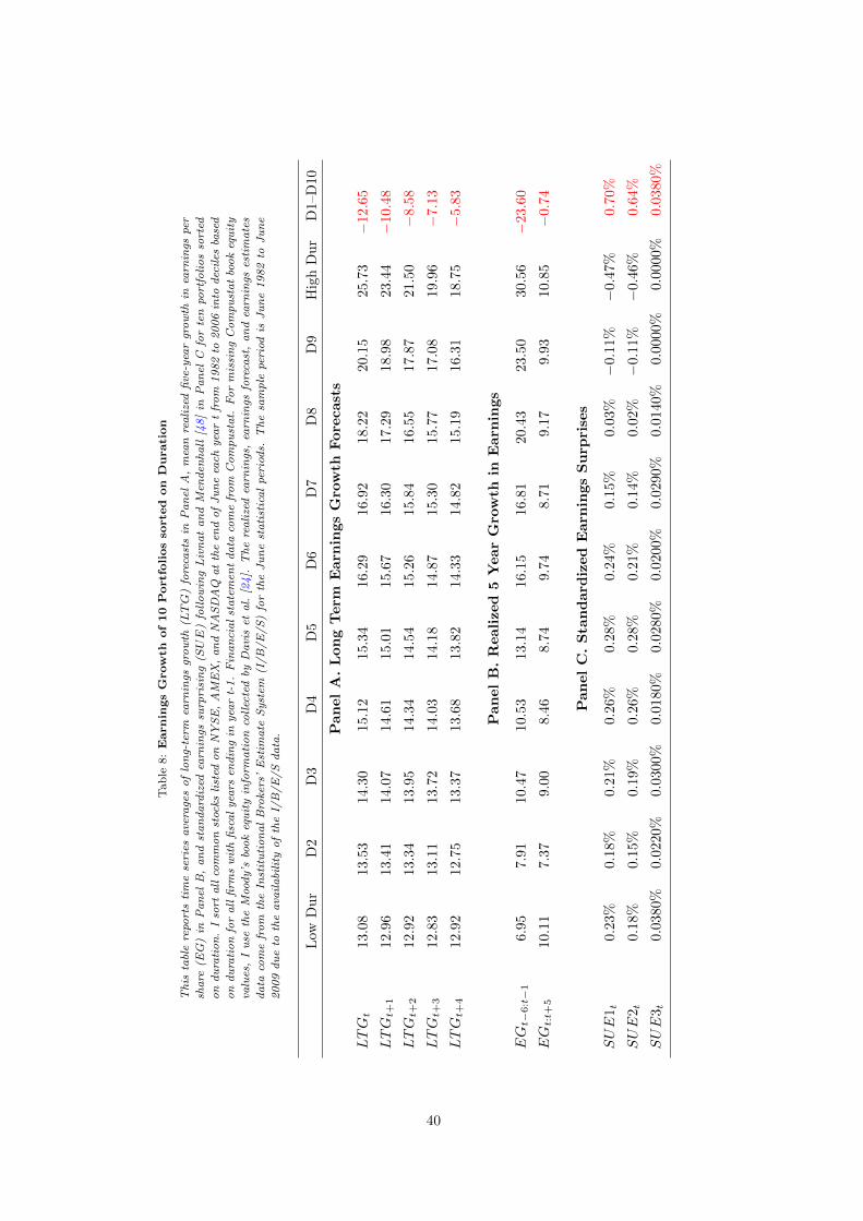
Tab

le8:Earnin

gsGrowth

of10

Portfoliosso

rte

don

Duration

Th

ista

ble

repo

rts

tim

ese

ries

ave

rage

so

flo

ng-

term

earn

ings

gro

wth

(LTG

)fo

reca

sts

inP

an

elA

,m

ean

rea

lize

dfi

ve-y

ear

gro

wth

inea

rnin

gspe

r

sha

re(E

G)

inP

an

elB

,a

nd

sta

nd

ard

ized

earn

ings

surp

risi

ng

(SUE

)fo

llo

win

gL

ivn

at

an

dM

end

enh

all

[48

]in

Pa

nel

Cfo

rte

npo

rtfo

lio

sso

rted

on

du

rati

on

.I

sort

all

com

mo

nst

ocks

list

edo

nN

YS

E,

AM

EX

,a

nd

NA

SD

AQ

at

the

end

of

Ju

ne

each

yea

rt

fro

m1

98

2to

20

06

into

dec

iles

base

d

on

du

rati

on

for

all

firm

sw

ith

fisc

al

yea

rsen

din

gin

yea

rt-

1.

Fin

an

cia

lst

ate

men

td

ata

com

efr

om

Co

mp

ust

at.

Fo

rm

issi

ng

Co

mp

ust

at

boo

keq

uit

y

valu

es,

Iu

seth

eM

ood

y’s

boo

keq

uit

yin

form

ati

on

coll

ecte

dby

Da

vis

eta

l.[2

4].

Th

ere

ali

zed

earn

ings

,ea

rnin

gsfo

reca

st,

an

dea

rnin

gses

tim

ate

s

da

taco

me

fro

mth

eIn

stit

uti

on

al

Bro

kers

’E

stim

ate

Syst

em(I

/B

/E

/S

)fo

rth

eJ

un

est

ati

stic

al

peri

ods.

Th

esa

mp

lepe

riod

isJ

un

e1

98

2to

Ju

ne

20

09

du

eto

the

ava

ila

bili

tyo

fth

eI/

B/

E/

Sd

ata

.

Low

Du

rD

2D

3D

4D

5D

6D

7D

8D

9H

igh

Du

rD

1–D

10

PanelA.LongTerm

Earn

ingsGro

wth

Fore

casts

LTG

t13.0

813.5

314.3

015.

12

15.3

416.2

916.9

218.2

220.1

525.7

3−

12.

65

LTG

t+1

12.9

613.4

114.0

714.

61

15.0

115.6

716.3

017.2

918.9

823.4

4−

10.

48

LTG

t+2

12.9

213.3

413.9

514.

34

14.5

415.2

615.8

416.5

517.8

721.5

0−

8.58

LTG

t+3

12.8

313.1

113.7

214.

03

14.1

814.8

715.3

015.7

717.0

819.9

6−

7.13

LTG

t+4

12.9

212.7

513.3

713.6

813.8

214.3

314.8

215.1

916.3

118.7

5−

5.83

PanelB.Realized

5YearGro

wth

inEarn

ings

EG

t−6:t−1

6.95

7.9

110.4

710.5

313.1

416.1

516.8

120.4

323.5

030.5

6−

23.

60

EG

t:t+

510.1

17.3

79.

008.4

68.7

49.7

48.7

19.1

79.9

310.8

5−

0.74

PanelC.Sta

ndard

ized

Earn

ingsSurp

rises

SUE

1t

0.23

%0.

18%

0.21

%0.

26%

0.28%

0.24%

0.15%

0.03%

−0.1

1%

−0.

47%

0.70%

SUE

2t

0.18

%0.

15%

0.19

%0.

26%

0.28%

0.21%

0.14%

0.02%

−0.1

1%

−0.

46%

0.64%

SUE

3t

0.03

80%

0.02

20%

0.03

00%

0.0180%

0.0280%

0.0200%

0.0290%

0.0140%

0.0000%

0.0000%

0.0380%

40

Table 9: Price Targets of 5 Portfolios sorted on Duration

This table reports time series averages of analysts twelve-months ahead price target scaled by the book value

of equity (PTB) and by the market price minus 1 (PTB) in Panel A, mean price-target implied expected

excess returns following periods of high and low investor sentiment Panel B, and benchmark-adjusted mean

price-target implied expected excess returns following periods of high and low investor sentiment Panel C for

five portfolios sorted on duration. I sort all common stocks listed on NYSE, AMEX, and NASDAQ at the

end of June each year t from 1982 to 2006 into deciles based on duration for all firms with fiscal years ending

in year t-1. I define high and low sentiment periods by the mean level of the sentiment index of Baker and

Wurgler [7]. Financial statement data come from Compustat. For missing Compustat book equity values,

I use the Moody’s book equity information collected by Davis et al. [24]. The realized earnings, earnings

forecast, and earnings estimates data come from the Institutional Brokers’ Estimate System (I/B/E/S) for

the June statistical periods. I use the Fama & French three-factor model as benchmark. The sample period

is July 2001 to June 2014 due to the availability of the target price data in Panel A and July 2001 to

December 2010 due to the availability of the sentiment index.

Low Dur D2 D3 D4 D5 D1–D5

Panel A. Scaled Price Targets

PTB 1.78 2.75 3.18 3.86 8.11 -6.33

PTP 16.83 15.83 14.92 14.66 16.85 -0.03

Panel B. Sentiment Means

meanHighSent 16.73 17.32 17.21 17.95 22.13 -5.41

(1.15) (0.97) (0.95) (0.91) (1.04) (0.76)

meanLowSent 17.88 15.45 14.87 14.09 15.43 2.44

(1.01) (0.85) (0.83) (0.80) (0.91) (0.67)

Panel C. Sentiment Alphas

αHighSent 16.49 16.94 16.82 17.49 21.61 -5.12

(1.09) (0.87) (0.87) (0.83) (0.98) (0.74)

αLowSent 18.81 16.53 15.84 15.05 16.32 2.48

(0.96) (0.77) (0.77) (0.73) (0.87) (0.66)

41

Table 10: Mean Excess Returns of 25 Portfolios sorted on Duration and Residual Institutional Ownership

This table reports monthly mean excess returns for twenty-five portfolios sorted on duration (Dur)

and residual institutional ownership (RIOR) with OLS standard errors in parentheses. I sort

all common stocks listed on NYSE, AMEX, and NASDAQ at the end of June each year t from

1981 to 2013 into quintiles based on duration for all firms with fiscal years ending in year t-1.

I intersect these quintiles with an independent sort on residual institutional ownership as of

December t-1. I weight returns equally and include delisting returns. If a firm is delisted for

cause (delisting code between 400 and 591) and has a missing delisting return, I assume a delisting

return of -30% following Shumway [60]. Dur is cash flow duration. RIOR is the residual in

a cross sectional regression of the fraction of shares held by institutions on size. Institutional

ownership information is obtained from the Thomson Reuters 13F database. Financial statement

data come from Compustat. For missing Compustat book equity values, I use the Moody’s book

equity information collected by Davis et al. [24]. I only use stocks above the 20th size percentile.

Low Dur D2 D3 D4 High Dur D1–D5

Mea

n

Low RIOR 1.02 0.84 0.75 0.47 -0.30 1.32

(0.29) (0.29) (0.29) (0.33) (0.45) (0.27)

RIOR2 1.08 0.96 0.85 0.73 0.25 0.83

(0.29) (0.28) (0.28) (0.29) (0.42) (0.24)

RIOR3 1.09 0.97 0.95 0.78 0.47 0.62

(0.29) (0.28) (0.28) (0.31) (0.42) (0.26)

RIOR4 1.04 1.02 0.91 0.64 0.52 0.52

(0.28) (0.29) (0.30) (0.33) (0.43) (0.27)

High RIOR 1.09 1.01 0.93 0.76 0.94 0.15

(0.31) (0.31) (0.31) (0.33) (0.42) (0.26)

RIOR1 – RIOR5 -0.08 -0.17 -0.18 -0.29 -1.24 1.17

(0.13) (0.13) (0.12) (0.13) (0.22) (0.23)

42

Tab

le11:Fam

a-French

Alp

hasof9

Portfoliosso

rte

don

Duration

and

ResidualIn

stitutionalOwnersh

ip(c

onditionalon

size)

Th

ista

ble

repo

rts

pri

cin

ger

rors

(α)

for

the

Fa

ma

&F

ren

chth

ree-

fact

or

mod

elfo

rn

ine

port

foli

os

sort

edo

nd

ura

tio

n(D

ur)

an

dre

sid

ua

l

inst

itu

tio

na

lo

wn

ersh

ip(R

IOR

)w

ith

OL

Sst

an

da

rder

rors

inpa

ren

thes

es,

sepa

rate

lyfo

rsm

all

stoc

ksin

Pa

nel

Ia

nd

larg

est

ocks

inP

an

el

II.

Iso

rta

llco

mm

on

stoc

ksli

sted

on

NY

SE

,A

ME

X,

an

dN

AS

DA

Qa

tth

een

do

fJ

un

eea

chyea

rt

fro

m1

98

1to

20

13

into

two

bask

ets

base

do

n

size

,a

nd

wit

hin

each

bin

Iso

rtst

ocks

into

tert

iles

base

do

nd

ura

tio

nfo

ra

llfi

rms

wit

hfi

sca

lyea

rsen

din

gin

yea

rt-

1.

Iin

ters

ect

thes

ete

rtil

es

wit

ha

nin

dep

end

ent

sort

on

resi

du

al

inst

itu

tio

na

lo

wn

ersh

ipa

so

fD

ecem

ber

t-1

.I

wei

ght

retu

rns

equ

all

ya

nd

incl

ud

ed

elis

tin

gre

turn

s.If

a

firm

isd

elis

ted

for

cau

se(d

elis

tin

gco

de

betw

een

40

0a

nd

59

1)

an

dh

as

am

issi

ng

del

isti

ng

retu

rn,

Ia

ssu

me

ad

elis

tin

gre

turn

of

-30

%fo

llo

win

g

Sh

um

wa

y[6

0].

Ma

rket

isth

eva

lue-

wei

ghte

dre

turn

on

all

NY

SE

,A

ME

X,

an

dN

AS

DA

Qco

mm

on

stoc

ksm

inu

sth

eo

ne-

mo

nth

Tre

asu

rybi

llra

te,

SMB

isth

ea

vera

gere

turn

on

thre

esm

all

port

foli

os

min

us

the

ave

rage

retu

rno

nth

ree

big

port

foli

os,

an

dHML

isth

ea

vera

gere

turn

on

two

valu

epo

rtfo

lio

sm

inu

sth

ea

vera

gere

turn

on

two

gro

wth

port

foli

os.

Du

ris

cash

flo

wd

ura

tio

n.

RIO

Ris

the

resi

du

al

ina

cro

ssse

ctio

na

lre

gres

sio

n

of

the

fra

ctio

no

fsh

are

sh

eld

byin

stit

uti

on

so

nsi

ze.

Inst

itu

tio

na

lo

wn

ersh

ipin

form

ati

on

iso

bta

ined

fro

mth

eT

ho

mso

nR

eute

rs1

3F

da

taba

se.

Fin

an

cia

lst

ate

men

td

ata

com

efr

om

Co

mp

ust

at.

Fo

rm

issi

ng

Co

mp

ust

at

boo

keq

uit

yva

lues

,I

use

the

Moo

dy’s

boo

keq

uit

yin

form

ati

on

coll

ecte

d

byD

avi

set

al.

[24

].I

on

lyu

sest

ocks

abo

veth

e2

0th

size

perc

enti

le.

Low

Du

rD

2H

igh

Du

rD

1–D

3L

owD

ur

D2

Hig

hD

ur

D1–D

3

PanelI.

Small

Sto

cks

PanelII.Larg

eSto

cks

αF&F

Low

RIO

R0.

980.3

0-0

.47

1.4

50.1

40.0

4-0

.58

0.7

2

(0.2

1)(0

.20)

(0.3

0)

(0.2

3)

(0.0

8)

(0.0

8)

(0.1

3)

(0.1

3)

RIO

R2

0.59

0.3

10.1

50.4

4-0

.06

0.0

3-0

.08

0.0

2

(0.1

5)(0

.14)

(0.2

7)

(0.2

0)

(0.0

9)

(0.0

8)

(0.1

1)

(0.1

1)

Hig

hR

IOR

0.58

0.4

40.6

5-0

.07

-0.0

20.0

4-0

.22

0.2

0

(0.1

6)(0

.15)

(0.3

1)

(0.2

5)

(0.1

0)

(0.1

0)

(0.1

2)

(0.1

3)

RIO

R1–

RIO

R3

0.40

-0.1

3-1

.13

1.5

20.1

60.0

0-0

.36

0.5

2

(0.1

7)(0

.15)

(0.2

2)

(0.2

7)

(0.0

9)

(0.0

8)

(0.1

4)

(0.1

4)

43

Tab

le12:Fam

a-French

Alp

hasof9

Portfoliosso

rte

don

Duration

and

ResidualIn

stitutionalOwnersh

ip(c

onditionalon

book-to-m

arket)

Th

ista

ble

repo

rts

pri

cin

ger

rors

(α)

for

the

Fa

ma

&F

ren

chth

ree-

fact

or

mod

elfo

rn

ine

port

foli

os

sort

edo

nd

ura

tio

n(D

ur)

an

dre

sid

ua

l

inst

itu

tio

na

lo

wn

ersh

ip(R

IOR

)w

ith

OL

Sst

an

da

rder

rors

inpa

ren

thes

es,

sepa

rate

lyfo

rgr

ow

thst

ocks

inP

an

elI

an

dva

lue

stoc

ksin

Pa

nel

II.

Iso

rta

llco

mm

on

stoc

ksli

sted

on

NY

SE

,A

ME

X,

an

dN

AS

DA

Qa

tth

een

do

fJ

un

eea

chyea

rt

fro

m1

98

1to

20

13

into

two

bask

ets

base

do

n

boo

k-to

-ma

rket

,a

nd

wit

hin

each

bin

Iso

rtst

ocks

into

tert

iles

base

do

nd

ura

tio

nfo

ra

llfi

rms

wit

hfi

sca

lyea

rsen

din

gin

yea

rt-

1.

Iin

ters

ect

thes

e

tert

iles

wit

ha

nin

dep

end

ent

sort

on

resi

du

al

inst

itu

tio

na

lo

wn

ersh

ipa

so

fD

ecem

ber

t-1

.I

wei

ght

retu

rns

equ

all

ya

nd

incl

ud

ed

elis

tin

gre

turn

s.If

afi

rmis

del

iste

dfo

rca

use

(del

isti

ng

cod

ebe

twee

n4

00

an

d5

91

)a

nd

ha

sa

mis

sin

gd

elis

tin

gre

turn

,I

ass

um

ea

del

isti

ng

retu

rno

f-3

0%

foll

ow

ing

Sh

um

wa

y[6

0].

Ma

rket

isth

eva

lue-

wei

ghte

dre

turn

on

all

NY

SE

,A

ME

X,

an

dN

AS

DA

Qco

mm

on

stoc

ksm

inu

sth

eo

ne-

mo

nth

Tre

asu

rybi

llra

te,

SMB

isth

ea

vera

gere

turn

on

thre

esm

all

port

foli

os

min

us

the

ave

rage

retu

rno

nth

ree

big

port

foli

os,

an

dHML

isth

ea

vera

gere

turn

on

two

valu

epo

rtfo

lio

sm

inu

sth

ea

vera

gere

turn

on

two

gro

wth

port

foli

os.

Du

ris

cash

flo

wd

ura

tio

n.

RIO

Ris

the

resi

du

al

ina

cro

ssse

ctio

na

lre

gres

sio

n

of

the

fra

ctio

no

fsh

are

sh

eld

byin

stit

uti

on

so

nsi

ze.

Inst

itu

tio

na

lo

wn

ersh

ipin

form

ati

on

iso

bta

ined

fro

mth

eT

ho

mso

nR

eute

rs1

3F

da

taba

se.

Fin

an

cia

lst

ate

men

td

ata

com

efr

om

Co

mp

ust

at.

Fo

rm

issi

ng

Co

mp

ust

at

boo

keq

uit

yva

lues

,I

use

the

Moo

dy’s

boo

keq

uit

yin

form

ati

on

coll

ecte

d

byD

avi

set

al.

[24

].I

on

lyu

sest

ocks

abo

veth

e2

0th

size

perc

enti

le.

Low

Du

rD

2H

igh

Du

rD

1–D

3L

owD

ur

D2

Hig

hD

ur

D1–D

3

PanelI.

Gro

wth

Sto

cks

PanelII.ValueSto

cks

αF&F

Low

RIO

R0.

06-0

.08

-0.9

00.9

50.8

10.4

00.1

90.6

3

(0.1

4)(0

.14)

(0.2

6)

(0.2

1)

(0.1

7)

(0.1

1)

(0.2

0)

(0.1

7)

RIO

R0.

150.0

6-0

.33

0.4

70.3

60.2

40.2

90.0

7

(0.0

8)(0

.08)

(0.2

2)

(0.2

2)

(0.1

2)

(0.0

9)

(0.1

5)

(0.1

2)

Hig

hR

IOR

0.08

-0.1

00.1

5-0

.07

0.5

30.1

80.3

80.1

4

(0.0

9)(0

.09)

(0.2

1)

(0.2

2)

(0.1

6)

(0.1

2)

(0.1

8)

(0.1

5)

RIO

R1–

RIO

R3

-0.0

20.0

2-1

.05

1.0

30.2

90.2

2-0

.20

0.4

8

(0.1

4)(0

.13)

(0.1

9)

(0.1

9)

(0.1

4)

(0.1

0)

(0.1

4)

(0.1

8)

44

Online Appendix:

Cash Flow Duration and750

the Term Structure of Equity Returns

Michael Weber

Not for Publication

1

Table A.1: Firm Names

This table reports five exemplary firm names for companies in the low- and high-duration portfolio in 1996 and

2004.

Panel I. 1996 Panel II. 2004

Low Duration High Duration Low Duration High Duration

Adolph Coors EA Industries Adolph Coors Enzo Biochem

Continental Peoplesoft Continental Adobe Systems

Chesapeake America Online Chesapeake Neurocrine Bioscs

United Industrial Symantec General Motors Penwest Pharma

Amcast Industrial McAfee SCS Transportation Martek Bioscs

2

Table A.2: Summary Statistics of 25 Portfolios sorted on Duration and Residual Institutional Ownership

This table reports time series averages of annual cross sectional means for firm characteristics and return predictors used

in the subsequent analysis for twenty-five portfolios sorted on duration (Dur) and residual institutional ownership (RIOR).

I sort all common stocks listed on NYSE, AMEX, and NASDAQ at the end of June each year t from 1981 to 2013 into

quintiles based on duration for all firms with fiscal years ending in year t-1. I intersected these quintiles with an independent

sort on residual institutional ownership as of December t-1. Dur is cash flow duration; BM is the book-to-market ratio;

IOR is the fraction of shares institutions hold; RIOR is the residual in a cross sectional regression of IOR on size; PR is

net payout over net income; ROE is return on equity; Sales g is sales growth; ME is the market capitalization in millions;

and Age is number of years a firm has been on Compustat. I obtain institutional ownership information from the Thomson

Reuters 13F database. Financial statement data come from Compustat. For missing Compustat book equity values, I use

the Moody’s book equity information collected by Davis et al. [24]. I only use stocks above the 20th size percentile.

Duration Duration

Low D2 D3 D4 High Low D2 D3 D4 High

Panel A. Dur Panel B. BM

Low RIOR 10.87 17.23 19.41 21.20 25.04 1.21 0.74 0.53 0.35 0.24

RIOR 2 11.70 17.19 19.38 21.18 24.61 1.21 0.75 0.53 0.35 0.27

RIOR 3 11.79 17.19 19.37 21.15 24.67 1.25 0.77 0.54 0.36 0.30

RIOR 4 11.48 17.14 19.38 21.13 24.47 1.34 0.80 0.57 0.41 0.33

High RIOR 11.18 17.10 19.36 21.13 24.53 1.47 0.87 0.63 0.45 0.40

Panel C. IOR Panel D. PR

Low RIOR 0.21 0.24 0.26 0.25 0.15 0.08 0.10 0.14 -0.14 -1.04

RIOR 2 0.37 0.41 0.44 0.45 0.34 0.29 0.30 0.19 0.00 -0.51

RIOR 3 0.42 0.48 0.52 0.53 0.42 0.25 0.21 0.08 -0.09 -0.75

RIOR 4 0.45 0.52 0.55 0.57 0.48 0.32 0.15 -0.02 -0.25 -0.74

High RIOR 0.55 0.60 0.63 0.64 0.59 0.27 0.06 -0.25 -0.48 -1.12

Panel E. ROE Panel F. Sales g

Low RIOR 0.42 0.16 0.16 0.17 -0.49 0.12 0.11 0.14 0.20 0.73

RIOR 2 0.27 0.14 0.15 0.18 -0.31 0.06 0.09 0.13 0.20 0.59

RIOR 3 0.20 0.12 0.14 0.16 -0.31 0.05 0.09 0.14 0.20 0.58

RIOR 4 0.16 0.10 0.12 0.13 -0.31 0.04 0.09 0.14 0.21 0.56

High RIOR 0.12 0.09 0.11 0.12 -0.35 0.03 0.09 0.14 0.22 0.51

Panel G. AGE Panel H. ME

Low RIOR 17.10 19.14 18.99 17.12 10.99 1639 1905 2588 2834 1224

RIOR 2 21.34 22.69 22.34 19.92 12.72 2304 2854 3791 4953 2451

RIOR 3 20.99 22.26 20.73 18.74 12.51 1565 2229 3022 4568 2529

RIOR 4 20.20 20.34 18.30 15.75 11.73 673 1305 1915 3251 1633

High RIOR 17.96 17.05 14.99 12.75 11.16 305 566 1151 1311 955

3

Table A.3: CAPM Alphas 25 Portfolios sorted on Duration and Residual Institutional Ownership

This table reports pricing errors (α) for the CAPM for twenty-five portfolios sorted on duration

(Dur) and residual institutional ownership (RIOR) with OLS standard errors in parentheses. I sort

all common stocks listed on NYSE, AMEX, and NASDAQ at the end of June each year t from

1981 to 2013 into quintiles based on duration for all firms with fiscal years ending in year t-1. I

intersect these quintiles with an independent sort on residual institutional ownership as of December

t-1. I weight returns equally and include delisting returns. If a firm is delisted for cause (delisting

code between 400 and 591) and has a missing delisting return, I assume a delisting return of -30%

following Shumway [60]. Market is the value weighted return on all NYSE, AMEX, and NASDAQ

common stocks minus the one-month Treasury bill rate, SMB is the average return on three small

portfolios minus the average return on three big portfolios, and HML is the average return on two

value portfolios minus the average return on two growth portfolios. Dur is cash flow duration. RIOR

is the residual in a cross sectional regression of the fraction of shares held by institutions on size.

Institutional ownership information is obtained from the Thomson Reuters 13F database. Financial

statement data come from Compustat. For missing Compustat book equity values, I use the Moody’s

book equity information collected by Davis et al. [24]. I only use stocks above the 20th size percentile.

Low Dur D2 D3 D4 High Dur D1–D5

αCAPM

Low RIOR 0.37 0.17 0.06 -0.29 -1.23 1.61

(0.19) (0.16) (0.15) (0.18) (0.32) (0.26)

RIOR2 0.40 0.26 0.14 -0.01 -0.69 1.09

(0.17) (0.14) (0.12) (0.12) (0.26) (0.23)

RIOR3 0.41 0.28 0.24 0.00 -0.47 0.88

(0.17) (0.14) (0.13) (0.14) (0.26) (0.25)

RIOR4 0.40 0.33 0.18 -0.17 -0.40 0.79

(0.17) (0.16) (0.15) (0.16) (0.28) (0.26)

High RIOR 0.42 0.30 0.21 -0.02 0.03 0.40

(0.20) (0.18) (0.18) (0.18) (0.27) (0.24)

RIOR1 – RIOR5 -0.05 -0.13 -0.15 -0.28 -1.26 1.21

(0.14) (0.13) (0.12) (0.13) (0.22) (0.23)

4

Table A.4: Fama - French Alphas of 25 Portfolios sorted on Duration and Residual Institutional Ownership

This table reports pricing errors (α) for the Fama & French three-factor model for twenty-five

portfolios sorted on duration (Dur) and residual institutional ownership (RIOR) with OLS standard

errors in parentheses. I sort all common stocks listed on NYSE, AMEX, and NASDAQ at the end

of June each year t from 1981 to 2013 into quintiles based on duration for all firms with fiscal years

ending in year t-1. I intersect these quintiles with an independent sort on residual institutional

ownership as of December t-1. I weight returns equally and include delisting returns. If a firm is

delisted for cause (delisting code between 400 and 591) and has a missing delisting return, I assume

a delisting return of -30% following Shumway [60]. Market is the value weighted return on all

NYSE, AMEX, and NASDAQ common stocks minus the one-month Treasury bill rate, SMB is the

average return on three small portfolios minus the average return on three big portfolios, HML is the

average return on two value portfolios minus the average return on two growth portfolios, and Mom

is the average return on two high prior return portfolios minus the average return on two low prior

return portfolios. Dur is cash flow duration. RIOR is the residual in a cross-sectional regression of

the fraction of shares held by institutions on size. Institutional ownership information is obtained

from the Thomson Reuters 13F database. Financial statement data come from Compustat. For

missing Compustat book equity values, I use the Moody’s book equity information collected by Davis

et al. [24]. I only use stocks above the 20th size percentile.

Low Dur D2 D3 D4 High Dur D1–D5

αF&F

Low RIOR 0.16 0.06 0.00 -0.22 -1.01 1.17

(0.13) (0.13) (0.11) (0.14) (0.24) (0.21)

RIOR2 0.17 0.12 0.05 0.03 -0.47 0.64

(0.12) (0.09) (0.08) (0.09) (0.18) (0.18)

RIOR3 0.12 0.05 0.14 0.05 -0.24 0.36

(0.11) (0.09) (0.09) (0.09) (0.18) (0.18)

RIOR4 0.13 0.12 0.05 -0.14 -0.16 0.29

(0.11) (0.09) (0.10) (0.11) (0.20) (0.20)

High RIOR 0.08 0.10 0.06 0.01 0.13 -0.05

(0.13) (0.11) (0.11) (0.13) (0.20) (0.20)

RIOR1–RIOR5 0.08 -0.04 -0.05 -0.23 -1.14 1.22

(0.13) (0.13) (0.12) (0.13) (0.22) (0.23)

5

Table A.5: Four Factor Alphas of 25 Portfolios sorted on Duration and Residual Institutional Ownership

This table reports pricing errors (α) for Fama & French three-factor model augmented with

momentum for twenty-five portfolios sorted on duration (Dur) and residual institutional ownership

(RIOR) with OLS standard errors in parentheses. I sort all common stocks listed on NYSE, AMEX,

and NASDAQ at the end of June each year t from 1981 to 2013 into quintiles based on duration

for all firms with fiscal years ending in year t-1. I intersect these quintiles with an independent

sort on residual institutional ownership as of December t-1. I weight returns equally and include

delisting returns. If a firm is delisted for cause (delisting code between 400 and 591) and has a

missing delisting return, I assume a delisting return of -30% following Shumway [60]. Market is the

value-weighted return on all NYSE, AMEX, and NASDAQ common stocks minus the one-month

Treasury bill rate, SMB is the average return on three small portfolios minus the average return

on three big portfolios, HML is the average return on two value portfolios minus the average

return on two growth portfolios, RMW is the average return on two robust operating profitability

portfolios minus the average return on two weak operating profitability portfolios, and CMA is the

average return on two conservative investment portfolios minus the average return on two aggressive

investment portfolios. Dur is cash flow duration. RIOR is the residual in a cross sectional regression

of the fraction of shares held by institutions on size. Institutional ownership information is obtained

from the Thomson Reuters 13F database. Financial statement data come from Compustat. For

missing Compustat book equity values, I use the Moody’s book equity information collected by Davis

et al. [24]. I only use stocks above the 20th size percentile.

Low Dur D2 D3 D4 High Dur D1–D5

α4Factor

Low RIOR 0.38 0.28 0.19 0.05 -0.56 0.94

(0.12) (0.11) (0.10) (0.12) (0.22) (0.20)

RIOR2 0.35 0.25 0.22 0.20 -0.10 0.45

(0.11) (0.08) (0.07) (0.08) (0.16) (0.18)

RIOR3 0.29 0.18 0.26 0.24 0.09 0.20

(0.10) (0.09) (0.08) (0.08) (0.16) (0.18)

RIOR4 0.28 0.25 0.22 0.08 0.17 0.11

(0.10) (0.09) (0.09) (0.09) (0.18) (0.20)

High RIOR 0.29 0.28 0.25 0.19 0.39 -0.10

(0.12) (0.10) (0.10) (0.12) (0.19) (0.21)

RIOR1–RIOR5 0.09 0.00 -0.06 -0.14 -0.95 1.04

(0.13) (0.13) (0.12) (0.14) (0.22) (0.23)

6

Table A.6: Five Factor Alphas of 25 Portfolios sorted on Duration and Residual Institutional Ownership

This table reports pricing errors (α) for the Fama & French five-factor model for twenty-five

portfolios sorted on duration (Dur) and residual institutional ownership (RIOR) with OLS standard

errors in parentheses. I sort all common stocks listed on NYSE, AMEX, and NASDAQ at the end

of June each year t from 1981 to 2013 into quintiles based on duration for all firms with fiscal years

ending in year t-1. I intersect these quintiles with an independent sort on residual institutional

ownership as of December t-1. I weight returns equally and include delisting returns. If a firm is

delisted for cause (delisting code between 400 and 591) and has a missing delisting return, I assume a

delisting return of -30% following Shumway [60]. Market is the value-weighted return on all NYSE,

AMEX, and NASDAQ stocks minus the one-month Treasury bill rate. Dur is cash flow duration.

RIOR is the residual in a cross sectional regression of the fraction of shares held by institutions

on size. Institutional ownership information is obtained from the Thomson Reuters 13F database.

Financial statement data come from Compustat. For missing Compustat book equity values, I use

the Moody’s book equity information collected by Davis et al. [24]. I only use stocks above the 20th

size percentile.

Low Dur D2 D3 D4 High Dur D1–D5

α5Factor

Low RIOR 0.23 0.14 0.08 -0.04 -0.43 0.66

(0.14) (0.13) (0.11) (0.14) (0.23) (0.19)

RIOR2 0.17 0.07 0.02 0.07 -0.07 0.24

(0.12) (0.09) (0.09) (0.09) (0.17) (0.16)

RIOR3 0.13 -0.04 0.07 0.12 0.05 0.08

(0.11) (0.09) (0.09) (0.10) (0.18) (0.18)

RIOR4 0.12 0.02 -0.01 -0.01 0.14 -0.02

(0.11) (0.09) (0.10) (0.11) (0.20) (0.19)

High RIOR 0.05 0.03 0.02 0.05 0.40 -0.35

(0.13) (0.11) (0.12) (0.13) (0.20) (0.20)

RIOR1–RIOR5 0.17 0.11 0.06 -0.09 -0.83 1.01

(0.14) (0.13) (0.12) (0.14) (0.23) (0.24)

7

Tab

leA

.7:Fam

a&

French

3Facto

rLoadin

gsof10

Portfoliosso

rte

don

Duration

Th

ista

ble

repo

rts

tim

ese

ries

fact

or

loa

din

gs(β

)fo

rth

eF

am

a&

Fre

nch

thre

e-fa

cto

rm

odel

for

ten

port

foli

os

sort

edo

nd

ura

tio

n(D

ur)

wit

hO

LS

sta

nd

ard

erro

rsin

pare

nth

eses

.I

sort

all

com

mo

nst

ocks

list

edo

nN

YS

E,

AM

EX

,a

nd

NA

SD

AQ

at

the

end

of

Ju

ne

each

yea

rt

fro

m1

96

3to

20

13

into

dec

iles

base

do

nd

ura

tio

nfo

ra

llfi

rms

wit

hfi

sca

lyea

rsen

din

gin

yea

rt-

1.

Iw

eigh

tre

turn

seq

ua

lly

an

din

clu

de

del

isti

ng

retu

rns.

Ifa

firm

isd

elis

ted

for

cau

se(d

elis

tin

gco

de

betw

een

40

0a

nd

59

1)

an

dh

as

am

issi

ng

del

isti

ng

retu

rn,

Ia

ssu

me

ad

elis

tin

gre

turn

of

-30

%fo

llo

win

g

Sh

um

wa

y[6

0].

Ma

rket

isth

eva

lue-

wei

ghte

dre

turn

on

all

NY

SE

,A

ME

X,

an

dN

AS

DA

Qco

mm

on

stoc

ksm

inu

sth

eo

ne-

mo

nth

Tre

asu

rybi

llra

te,

SMB

isth

ea

vera

gere

turn

on

thre

esm

all

port

foli

os

min

us

the

ave

rage

retu

rno

nth

ree

big

port

foli

os,

an

dHML

isth

ea

vera

gere

turn

on

two

valu

epo

rtfo

lio

sm

inu

sth

ea

vera

gere

turn

on

two

gro

wth

port

foli

os.

Du

ris

cash

flo

wd

ura

tio

n.

Fin

an

cia

lst

ate

men

td

ata

com

efr

om

Co

mp

ust

at.

Fo

rm

issi

ng

Co

mp

ust

at

boo

keq

uit

yva

lues

,I

use

the

Moo

dy’s

boo

keq

uit

yin

form

ati

on

coll

ecte

dby

Da

vis

eta

l.[2

4].

Low

Du

rD

2D

3D

4D

5D

6D

7D

8D

9H

igh

Du

rD

1–D

10

βM

arket

0.95

0.96

0.97

0.9

91.0

11.0

21.0

31.0

61.1

21.0

8-0

.13

(0.0

2)(0

.02)

(0.0

2)

(0.0

1)

(0.0

1)

(0.0

2)

(0.0

2)

(0.0

2)

(0.0

3)

(0.0

4)

(0.0

4)

βSM

B1.

030.

940.

92

0.8

70.8

50.8

50.8

50.8

60.9

91.2

1-0

.18

(0.0

2)(0

.02)

(0.0

2)

(0.0

1)

(0.0

1)

(0.0

2)

(0.0

2)

(0.0

2)

(0.0

3)

(0.0

4)

(0.0

4)

βH

ML

0.53

0.43

0.37

0.3

20.2

20.1

70.0

4-0

.16

-0.3

9-0

.49

1.0

2

(0.0

2)(0

.02)

(0.0

2)

(0.0

1)

(0.0

1)

(0.0

2)

(0.0

2)

(0.0

2)

(0.0

3)

(0.0

4)

(0.0

4)

8

Tab

leA

.8:Fam

a&

French

4Facto

rLoadin

gsof10

Portfoliosso

rte

don

Duration

Th

ista

ble

repo

rts

tim

ese

ries

fact

or

loa

din

gs(β

)fo

rth

eF

am

a&

Fre

nch

thre

e-fa

cto

rm

odel

au

gmen

ted

bym

om

entu

mfo

rte

npo

rtfo

lio

sso

rted

on

du

rati

on

(Du

r)w

ith

OL

Sst

an

da

rder

rors

inpa

ren

thes

es.

Iso

rta

llco

mm

on

stoc

ksli

sted

on

NY

SE

,A

ME

X,

an

dN

AS

DA

Qa

tth

een

do

f

Ju

ne

each

yea

rt

fro

m1

96

3to

20

13

into

dec

iles

base

do

nd

ura

tio

nfo

ra

llfi

rms

wit

hfi

sca

lyea

rsen

din

gin

yea

rt-

1.

Iw

eigh

tre

turn

seq

ua

lly

an

din

clu

de

del

isti

ng

retu

rns.

Ifa

firm

isd

elis

ted

for

cau

se(d

elis

tin

gco

de

betw

een

40

0a

nd

59

1)

an

dh

as

am

issi

ng

del

isti

ng

retu

rn,

Ia

ssu

me

a

del

isti

ng

retu

rno

f-3

0%

foll

ow

ing

Sh

um

wa

y[6

0].

Ma

rket

isth

eva

lue-

wei

ghte

dre

turn

on

all

NY

SE

,A

ME

X,

an

dN

AS

DA

Qco

mm

on

stoc

ksm

inu

s

the

on

e-m

on

thT

rea

sury

bill

rate

,SMB

isth

ea

vera

gere

turn

on

thre

esm

all

port

foli

os

min

us

the

ave

rage

retu

rno

nth

ree

big

port

foli

os,HML

is

the

ave

rage

retu

rno

ntw

ova

lue

port

foli

os

min

us

the

ave

rage

retu

rno

ntw

ogr

ow

thpo

rtfo

lio

s,a

ndMom

isth

ea

vera

gere

turn

on

two

hig

hp

rio

r

retu

rnpo

rtfo

lio

sm

inu

sth

ea

vera

gere

turn

on

two

low

pri

or

retu

rnpo

rtfo

lio

s.D

ur

isca

shfl

ow

du

rati

on

.F

ina

nci

al

sta

tem

ent

da

taco

me

fro

m

Co

mp

ust

at.

Fo

rm

issi

ng

Co

mp

ust

at

boo

keq

uit

yva

lues

,I

use

the

Moo

dy’s

boo

keq

uit

yin

form

ati

on

coll

ecte

dby

Da

vis

eta

l.[2

4].

Low

Du

rD

2D

3D

4D

5D

6D

7D

8D

9H

igh

Du

rD

1–D

10

βM

arket

0.92

0.93

0.95

0.9

70.9

80.9

91.0

01.0

21.0

71.0

2-0

.10

(0.0

2)(0

.02)

(0.0

2)

(0.0

1)

(0.0

1)

(0.0

1)

(0.0

1)

(0.0

2)

(0.0

2)

(0.0

4)

(0.0

4)

βSM

B1.

030.

940.

92

0.8

70.8

50.8

50.8

50.8

60.9

91.2

1-0

.19

(0.0

3)(0

.02)

(0.0

2)

(0.0

2)

(0.0

2)

(0.0

2)

(0.0

2)

(0.0

2)

(0.0

3)

(0.0

6)

(0.0

5)

βH

ML

0.48

0.38

0.33

0.2

70.1

70.1

2-0

.02

-0.2

3-0

.48

-0.6

01.0

8

(0.0

3)(0

.03)

(0.0

2)

(0.0

2)

(0.0

2)

(0.0

2)

(0.0

2)

(0.0

2)

(0.0

3)

(0.0

6)

(0.0

5)

βM

om

-0.1

5-0

.17

-0.1

4-0

.15

-0.1

5-0

.18

-0.1

9-0

.21

-0.2

9-0

.35

0.2

0

(0.0

2)(0

.02)

(0.0

1)

(0.0

1)

(0.0

1)

(0.0

1)

(0.0

1)

(0.0

1)

(0.0

2)

(0.0

4)

(0.0

4)

9

Tab

leA

.9:Fam

a&

French

5Facto

rLoadin

gsof10

Portfoliosso

rte

don

Duration

Th

ista

ble

repo

rts

tim

ese

ries

fact

or

loa

din

gs(β

)fo

rth

eF

am

a&

Fre

nch

five

-fa

cto

rm

odel

for

ten

port

foli

os

sort

edo

nd

ura

tio

n(D

ur)

wit

hO

LS

sta

nd

ard

erro

rsin

pare

nth

eses

.I

sort

all

com

mo

nst

ocks

list

edo

nN

YS

E,

AM

EX

,a

nd

NA

SD

AQ

at

the

end

of

Ju

ne

each

yea

rt

fro

m1

96

3to

20

13

into

dec

iles

base

do

nd

ura

tio

nfo

ra

llfi

rms

wit

hfi

sca

lyea

rsen

din

gin

yea

rt-

1.

Iw

eigh

tre

turn

seq

ua

lly

an

din

clu

de

del

isti

ng

retu

rns.

Ifa

firm

isd

elis

ted

for

cau

se(d

elis

tin

gco

de

betw

een

40

0a

nd

59

1)

an

dh

as

am

issi

ng

del

isti

ng

retu

rn,

Ia

ssu

me

ad

elis

tin

gre

turn

of

-30

%fo

llo

win

g

Sh

um

wa

y[6

0].

Ma

rket

isth

eva

lue-

wei

ghte

dre

turn

on

all

NY

SE

,A

ME

X,

an

dN

AS

DA

Qco

mm

on

stoc

ksm

inu

sth

eo

ne-

mo

nth

Tre

asu

rybi

llra

te,

SMB

isth

ea

vera

gere

turn

on

thre

esm

all

port

foli

os

min

us

the

ave

rage

retu

rno

nth

ree

big

port

foli

os,HML

isth

ea

vera

gere

turn

on

two

valu

e

port

foli

os

min

us

the

ave

rage

retu

rno

ntw

ogr

ow

thpo

rtfo

lio

s,RMW

isth

ea

vera

gere

turn

on

two

robu

sto

pera

tin

gp

rofi

tabi

lity

port

foli

os

min

us

the

ave

rage

retu

rno

ntw

ow

eak

ope

rati

ng

pro

fita

bili

typo

rtfo

lio

s,a

ndCMA

isth

ea

vera

gere

turn

on

two

con

serv

ati

vein

vest

men

tpo

rtfo

lio

sm

inu

s

the

ave

rage

retu

rno

ntw

oa

ggre

ssiv

ein

vest

men

tpo

rtfo

lio

s.D

ur

isca

shfl

ow

du

rati

on

.F

ina

nci

al

sta

tem

ent

da

taco

me

fro

mC

om

pu

sta

t.F

or

mis

sin

gC

om

pu

sta

tbo

ok

equ

ity

valu

es,

Iu

seth

eM

ood

y’s

boo

keq

uit

yin

form

ati

on

coll

ecte

dby

Da

vis

eta

l.[2

4].

Low

Du

rD

2D

3D

4D

5D

6D

7D

8D

9H

igh

Du

rD

1–D

10

βM

arket

0.95

0.95

0.97

0.9

91.0

11.0

11.0

31.0

31.0

71.0

1-0

.06

(0.0

2)(0

.02)

(0.0

2)

(0.0

2)

(0.0

2)

(0.0

2)

(0.0

2)

(0.0

2)

(0.0

2)

(0.0

4)

(0.0

3)

βSM

B1.

000.

930.

92

0.8

80.8

50.8

50.8

30.8

10.8

70.9

80.0

2

(0.0

3)(0

.03)

(0.0

2)

(0.0

2)

(0.0

2)

(0.0

2)

(0.0

2)

(0.0

2)

(0.0

3)

(0.0

6)

(0.0

5)

βH

ML

0.52

0.44

0.35

0.3

20.2

10.2

00.0

7-0

.10

-0.2

9-0

.36

0.8

8

(0.0

5)(0

.04)

(0.0

3)

(0.0

3)

(0.0

3)

(0.0

3)

(0.0

3)

(0.0

3)

(0.0

5)

(0.0

8)

(0.0

7)

βRM

W-0

.10

-0.0

4-0

.02

0.0

5-0

.01

0.0

0-0

.08

-0.2

3-0

.54

-1.0

10.9

0

(0.0

5)(0

.04)

(0.0

3)

(0.0

3)

(0.0

3)

(0.0

3)

(0.0

3)

(0.0

4)

(0.0

5)

(0.0

9)

(0.0

7)

βCM

A0.

02-0

.01

0.04

-0.0

10.0

1-0

.05

-0.0

6-0

.13

-0.2

0-0

.27

0.2

9

(0.0

7)(0

.06)

(0.0

5)

(0.0

5)

(0.0

4)

(0.0

5)

(0.0

5)

(0.0

5)

(0.0

7)

(0.1

2)

(0.1

0)

10

Tab

leA

.10:CAPM

Loadin

gsof10

Portfoliosso

rte

don

Duration:Volatility

-managed

Portfolios

Th

ista

ble

repo

rts

tim

ese

ries

fact

or

loa

din

gs(β

)fo

rth

eF

am

a&

Fre

nch

thre

e-fa

cto

rm

odel

for

ten

port

foli

os

sort

edo

nd

ura

tio

n(D

ur)

wit

hO

LS

sta

nd

ard

erro

rsin

pare

nth

eses

.P

ort

foli

ore

turn

sa

resc

ale

dby

the

pre

vio

us

mo

nth

sre

ali

zed

vari

an

cea

sin

Mo

reir

aa

nd

Mu

ir[5

4].

Iso

rta

ll

com

mo

nst

ocks

list

edo

nN

YS

E,

AM

EX

,a

nd

NA

SD

AQ

at

the

end

of

Ju

ne

each

yea

rt

fro

m1

96

3to

20

13

into

dec

iles

base

do

nd

ura

tio

nfo

ra

llfi

rms

wit

hfi

sca

lyea

rsen

din

gin

yea

rt-

1.

Iw

eigh

tre

turn

seq

ua

lly

an

din

clu

de

del

isti

ng

retu

rns.

Ifa

firm

isd

elis

ted

for

cau

se(d

elis

tin

gco

de

betw

een

40

0a

nd

59

1)

an

dh

as

am

issi

ng

del

isti

ng

retu

rn,

Ia

ssu

me

ad

elis

tin

gre

turn

of

-30

%fo

llo

win

gS

hu

mw

ay

[60

].M

ark

etis

the

valu

e-w

eigh

ted

retu

rno

na

llN

YS

E,

AM

EX

,a

nd

NA

SD

AQ

com

mo

nst

ocks

min

us

the

on

e-m

on

thT

rea

sury

bill

rate

,SMB

isth

ea

vera

gere

turn

on

thre

esm

all

port

foli

os

min

us

the

ave

rage

retu

rno

nth

ree

big

port

foli

os,

an

dHML

isth

ea

vera

gere

turn

on

two

valu

epo

rtfo

lio

sm

inu

sth

ea

vera

gere

turn

on

two

gro

wth

port

foli

os.

Du

ris

cash

flo

wd

ura

tio

n.

Fin

an

cia

lst

ate

men

td

ata

com

efr

om

Co

mp

ust

at.

Fo

rm

issi

ng

Co

mp

ust

at

boo

keq

uit

yva

lues

,I

use

the

Moo

dy’s

boo

keq

uit

yin

form

ati

on

coll

ecte

dby

Da

vis

eta

l.[2

4].

Low

Du

rD

2D

3D

4D

5D

6D

7D

8D

9H

igh

Du

rD

1–D

10

βM

arket

0.81

0.76

0.79

0.7

60.8

30.8

20.8

20.9

11.0

01.1

0-0

.26

(0.0

5)(0

.04)

(0.0

4)

(0.0

4)

(0.0

4)

(0.0

4)

(0.0

4)

(0.0

4)

(0.0

5)

(0.0

6)

(0.0

4)

11

Tab

leA

.11:Fam

a&

French

3Facto

rLoadin

gsof10

Portfoliosso

rte

don

Duration:Volatility

-managed

Portfolios

Th

ista

ble

repo

rts

tim

ese

ries

fact

or

loa

din

gs(β

)fo

rth

eF

am

a&

Fre

nch

thre

e-fa

cto

rm

odel

for

ten

port

foli

os

sort

edo

nd

ura

tio

n(D

ur)

wit

hO

LS

sta

nd

ard

erro

rsin

pare

nth

eses

.P

ort

foli

ore

turn

sa

resc

ale

dby

the

pre

vio

us

mo

nth

sre

ali

zed

vari

an

cea

sin

Mo

reir

aa

nd

Mu

ir[5

4].

Iso

rta

ll

com

mo

nst

ocks

list

edo

nN

YS

E,

AM

EX

,a

nd

NA

SD

AQ

at

the

end

of

Ju

ne

each

yea

rt

fro

m1

96

3to

20

13

into

dec

iles

base

do

nd

ura

tio

nfo

ra

llfi

rms

wit

hfi

sca

lyea

rsen

din

gin

yea

rt-

1.

Iw

eigh

tre

turn

seq

ua

lly

an

din

clu

de

del

isti

ng

retu

rns.

Ifa

firm

isd

elis

ted

for

cau

se(d

elis

tin

gco

de

betw

een

40

0a

nd

59

1)

an

dh

as

am

issi

ng

del

isti

ng

retu

rn,

Ia

ssu

me

ad

elis

tin

gre

turn

of

-30

%fo

llo

win

gS

hu

mw

ay

[60

].M

ark

etis

the

valu

e-w

eigh

ted

retu

rno

na

llN

YS

E,

AM

EX

,a

nd

NA

SD

AQ

com

mo

nst

ocks

min

us

the

on

e-m

on

thT

rea

sury

bill

rate

,SMB

isth

ea

vera

gere

turn

on

thre

esm

all

port

foli

os

min

us

the

ave

rage

retu

rno

nth

ree

big

port

foli

os,

an

dHML

isth

ea

vera

gere

turn

on

two

valu

epo

rtfo

lio

sm

inu

sth

ea

vera

gere

turn

on

two

gro

wth

port

foli

os.

Du

ris

cash

flo

wd

ura

tio

n.

Fin

an

cia

lst

ate

men

td

ata

com

efr

om

Co

mp

ust

at.

Fo

rm

issi

ng

Co

mp

ust

at

boo

keq

uit

yva

lues

,I

use

the

Moo

dy’s

boo

keq

uit

yin

form

ati

on

coll

ecte

dby

Da

vis

eta

l.[2

4].

Low

Du

rD

2D

3D

4D

5D

6D

7D

8D

9H

igh

Du

rD

1–D

10

βM

arket

0.70

0.67

0.69

0.6

80.7

30.7

30.7

10.7

80.8

30.8

7-0

.11

(0.0

4)(0

.04)

(0.0

4)

(0.0

4)

(0.0

4)

(0.0

4)

(0.0

4)

(0.0

5)

(0.0

5)

(0.0

6)

(0.0

4)

βSM

B0.

730.

600.

62

0.5

20.5

60.5

50.5

80.6

10.7

60.9

9-0

.13

(0.0

6)(0

.06)

(0.0

6)

(0.0

6)

(0.0

6)

(0.0

6)

(0.0

6)

(0.0

6)

(0.0

8)

(0.0

9)

(0.0

6)

βH

ML

0.17

0.12

0.14

0.1

10.0

50.0

50.0

1-0

.09

-0.0

9-0

.19

0.6

2

(0.0

7)(0

.07)

(0.0

6)

(0.0

7)

(0.0

6)

(0.0

6)

(0.0

7)

(0.0

7)

(0.0

8)

(0.1

0)

(0.0

7)

12

Tab

leA

.12:Fam

a&

French

4Facto

rLoadin

gsof10

Portfoliosso

rte

don

Duration:Volatility

-managed

Portfolios

Th

ista

ble

repo

rts

tim

ese

ries

fact

or

loa

din

gs(β

)fo

rth

eF

am

a&

Fre

nch

thre

e-fa

cto

rm

odel

au

gmen

ted

bym

om

entu

mfo

rte

npo

rtfo

lio

sso

rted

on

du

rati

on

(Du

r)w

ith

OL

Sst

an

da

rder

rors

inpa

ren

thes

es.

Po

rtfo

lio

retu

rns

are

sca

led

byth

ep

revi

ou

sm

on

ths

rea

lize

dva

ria

nce

as

inM

ore

ira

an

d

Mu

ir[5

4].

Iso

rta

llco

mm

on

stoc

ksli

sted

on

NY

SE

,A

ME

X,

an

dN

AS

DA

Qa

tth

een

do

fJ

un

eea

chyea

rt

fro

m1

96

3to

20

13

into

dec

iles

base

d

on

du

rati

on

for

all

firm

sw

ith

fisc

al

yea

rsen

din

gin

yea

rt-

1.

Iw

eigh

tre

turn

seq

ua

lly

an

din

clu

de

del

isti

ng

retu

rns.

Ifa

firm

isd

elis

ted

for

cau

se

(del

isti

ng

cod

ebe

twee

n4

00

an

d5

91

)a

nd

ha

sa

mis

sin

gd

elis

tin

gre

turn

,I

ass

um

ea

del

isti

ng

retu

rno

f-3

0%

foll

ow

ing

Sh

um

wa

y[6

0].

Ma

rket

isth

eva

lue-

wei

ghte

dre

turn

on

all

NY

SE

,A

ME

X,

an

dN

AS

DA

Qco

mm

on

stoc

ksm

inu

sth

eo

ne-

mo

nth

Tre

asu

rybi

llra

te,SMB

isth

ea

vera

ge

retu

rno

nth

ree

sma

llpo

rtfo

lio

sm

inu

sth

ea

vera

gere

turn

on

thre

ebi

gpo

rtfo

lio

s,HML

isth

ea

vera

gere

turn

on

two

valu

epo

rtfo

lio

sm

inu

sth

e

ave

rage

retu

rno

ntw

ogr

ow

thpo

rtfo

lio

s,a

ndMom

isth

ea

vera

gere

turn

on

two

hig

hp

rio

rre

turn

port

foli

os

min

us

the

ave

rage

retu

rno

ntw

olo

w

pri

or

retu

rnpo

rtfo

lio

s.D

ur

isca

shfl

ow

du

rati

on

.F

ina

nci

al

sta

tem

ent

da

taco

me

fro

mC

om

pu

sta

t.F

or

mis

sin

gC

om

pu

sta

tbo

ok

equ

ity

valu

es,

I

use

the

Moo

dy’s

boo

keq

uit

yin

form

ati

on

coll

ecte

dby

Da

vis

eta

l.[2

4].

Low

Du

rD

2D

3D

4D

5D

6D

7D

8D

9H

igh

Du

rD

1–D

10

βM

arket

0.72

0.69

0.71

0.7

00.7

50.7

50.7

40.8

10.8

60.9

0-0

.10

(0.0

5)(0

.04)

(0.0

4)

(0.0

4)

(0.0

4)

(0.0

4)

(0.0

4)

(0.0

5)

(0.0

5)

(0.0

6)

(0.0

4)

βSM

B0.

730.

600.

62

0.5

20.5

50.5

50.5

80.6

10.7

60.9

9-0

.13

(0.0

6)(0

.06)

(0.0

6)

(0.0

6)

(0.0

6)

(0.0

6)

(0.0

6)

(0.0

6)

(0.0

7)

(0.0

9)

(0.0

6)

βH

ML

0.21

0.16

0.18

0.1

40.1

00.0

90.0

5-0

.04

-0.0

4-0

.13

0.6

4

(0.0

7)(0

.07)

(0.0

6)

(0.0

7)

(0.0

6)

(0.0

7)

(0.0

7)

(0.0

7)

(0.0

8)

(0.1

0)

(0.0

7)

βM

om

0.11

0.11

0.12

0.1

20.1

50.1

30.1

50.1

70.1

70.1

80.0

6

(0.0

4)(0

.04)

(0.0

4)

(0.0

4)

(0.0

4)

(0.0

4)

(0.0

4)

(0.0

4)

(0.0

5)

(0.0

6)

(0.0

4)

13

Tab

leA

.13:Fam

a&

French

5Facto

rLoadin

gsof10

Portfoliosso

rte

don

Duration:Volatility

-managed

Portfolios

Th

ista

ble

repo

rts

tim

ese

ries

fact

or

loa

din

gs(β

)fo

rth

eF

am

a&

Fre

nch

five

-fa

cto

rm

odel

for

ten

port

foli

os

sort

edo

nd

ura

tio

n(D

ur)

wit

hO

LS

sta

nd

ard

erro

rsin

pare

nth

eses

.P

ort

foli

ore

turn

sa

resc

ale

dby

the

pre

vio

us

mo

nth

sre

ali

zed

vari

an

cea

sin

Mo

reir

aa

nd

Mu

ir[5

4].

Iso

rta

ll

com

mo

nst

ocks

list

edo

nN

YS

E,

AM

EX

,a

nd

NA

SD

AQ

at

the

end

of

Ju

ne

each

yea

rt

fro

m1

96

3to

20

13

into

dec

iles

base

do

nd

ura

tio

nfo

ra

llfi

rms

wit

hfi

sca

lyea

rsen

din

gin

yea

rt-

1.

Iw

eigh

tre

turn

seq

ua

lly

an

din

clu

de

del

isti

ng

retu

rns.

Ifa

firm

isd

elis

ted

for

cau

se(d

elis

tin

gco

de

betw

een

40

0a

nd

59

1)

an

dh

as

am

issi

ng

del

isti

ng

retu

rn,

Ia

ssu

me

ad

elis

tin

gre

turn

of

-30

%fo

llo

win

gS

hu

mw

ay

[60

].M

ark

etis

the

valu

e-w

eigh

ted

retu

rno

na

llN

YS

E,

AM

EX

,a

nd

NA

SD

AQ

com

mo

nst

ocks

min

us

the

on

e-m

on

thT

rea

sury

bill

rate

,SMB

isth

ea

vera

gere

turn

on

thre

esm

all

port

foli

os

min

us

the

ave

rage

retu

rno

nth

ree

big

port

foli

os,HML

isth

ea

vera

gere

turn

on

two

valu

epo

rtfo

lio

sm

inu

sth

ea

vera

gere

turn

on

two

gro

wth

port

foli

os,RMW

isth

ea

vera

gere

turn

on

two

robu

sto

pera

tin

gp

rofi

tabi

lity

port

foli

os

min

us

the

ave

rage

retu

rno

ntw

ow

eak

ope

rati

ng

pro

fita

bili

typo

rtfo

lio

s,a

ndCMA

isth

ea

vera

gere

turn

on

two

con

serv

ati

vein

vest

men

tpo

rtfo

lio

sm

inu

sth

ea

vera

gere

turn

on

two

agg

ress

ive

inve

stm

ent

port

foli

os.

Du

ris

cash

flo

wd

ura

tio

n.

Fin

an

cia

lst

ate

men

td

ata

com

efr

om

Co

mp

ust

at.

Fo

rm

issi

ng

Co

mp

ust

at

boo

keq

uit

yva

lues

,I

use

the

Moo

dy’s

boo

keq

uit

yin

form

ati

on

coll

ecte

dby

Da

vis

eta

l.[2

4].

Low

Du

rD

2D

3D

4D

5D

6D

7D

8D

9H

igh

Du

rD

1–D

10

βM

arket

0.76

0.72

0.74

0.7

20.7

60.7

60.7

50.8

20.8

80.9

2-0

.10

(0.0

5)(0

.05)

(0.0

4)

(0.0

5)

(0.0

4)

(0.0

4)

(0.0

5)

(0.0

5)

(0.0

6)

(0.0

7)

(0.0

5)

βSM

B0.

770.

660.

66

0.5

70.6

20.6

10.6

40.6

80.8

41.0

3-0

.09

(0.0

7)(0

.06)

(0.0

6)

(0.0

6)

(0.0

6)

(0.0

6)

(0.0

7)

(0.0

7)

(0.0

8)

(0.0

9)

(0.0

7)

βH

ML

-0.0

4-0

.07

-0.0

4-0

.02

-0.0

5-0

.07

-0.1

2-0

.23

-0.2

6-0

.39

0.6

2

(0.0

9)(0

.09)

(0.0

9)

(0.0

9)

(0.0

8)

(0.0

9)

(0.0

9)

(0.0

9)

(0.1

1)

(0.1

3)

(0.0

9)

βRM

W0.

200.

270.

22

0.2

40.2

80.2

80.2

80.3

30.3

40.1

60.1

9

(0.1

0)(0

.09)

(0.0

9)

(0.0

9)

(0.0

9)

(0.0

9)

(0.1

0)

(0.1

0)

(0.1

1)

(0.1

4)

(0.1

0)

βCM

A0.

460.

430.

39

0.2

80.2

10.2

40.2

70.2

90.3

60.4

50.0

0

(0.1

4)(0

.13)

(0.1

3)

(0.1

3)

(0.1

3)

(0.1

3)

(0.1

4)

(0.1

4)

(0.1

6)

(0.2

0)

(0.1

4)

14

Table A.14: CAPM Betas of 25 Portfolios sorted on Duration and Residual Institutional Ownership

This table reports time series factor loadings (β) for the CAPM for twenty-five portfolios sorted on

duration (Dur) and residual institutional ownership (RIOR) with OLS standard errors in parentheses.

I sort all common stocks listed on NYSE, AMEX, and NASDAQ at the end of June each year t from

1981 to 2013 into quintiles based on duration for all firms with fiscal years ending in year t-1. I intersect

these quintiles with an independent sort on residual institutional ownership as of December t-1. I weight

returns equally and include delisting returns. If a firm is delisted for cause (delisting code between 400

and 591) and has a missing delisting return, I assume a delisting return of -30% following Shumway

[60]. Market is the value-weighted return on all NYSE, AMEX, and NASDAQ common stocks minus

the one-month Treasury bill rate. Dur is cash flow duration. Financial statement data come from

Compustat. For missing Compustat book equity values, I use the Moody’s book equity information

collected by Davis et al. [24]. I only use stocks above the 20th size percentile.

Low Dur D2 D3 D4 High Dur D1–D5

βCAPM

Low RIOR 1.01 1.05 1.08 1.20 1.46 -0.45

(0.04) (0.04) (0.03) (0.04) (0.07) (0.06)

RIOR2 1.06 1.09 1.12 1.16 1.47 -0.41

(0.04) (0.03) (0.03) (0.03) (0.06) (0.05)

RIOR3 1.06 1.09 1.11 1.21 1.47 -0.41

(0.04) (0.03) (0.03) (0.03) (0.06) (0.05)

RIOR4 1.01 1.09 1.15 1.26 1.45 -0.44

(0.04) (0.04) (0.03) (0.04) (0.06) (0.06)

High RIOR 1.05 1.10 1.14 1.22 1.43 -0.38

(0.04) (0.04) (0.04) (0.04) (0.06) (0.05)

RIOR1–RIOR5 -0.04 -0.05 -0.06 -0.02 0.03 -0.07

(0.03) (0.03) (0.03) (0.03) (0.05) (0.05)

15

Table A.15: Fama & French Factor loadings of 25 Portfolios sorted on Duration and Residual InstitutionalOwnership

This table reports time series factor loadings (β) for the Fama & French three-factor model for twenty-five

portfolios sorted on duration (Dur) and residual institutional ownership (RIOR) with OLS standard errors

in parentheses. I sort all common stocks listed on NYSE, AMEX, and NASDAQ at the end of June each

year t from 1981 to 2013 into quintiles based on duration for all firms with fiscal years ending in year t-1.

I intersect these quintiles with an independent sort on residual institutional ownership as of December t-1.

I weight returns equally and include delisting returns. If a firm is delisted for cause (delisting code between

400 and 591) and has a missing delisting return, I assume a delisting return of -30% following Shumway

[60]. Market is the value-weighted return on all NYSE, AMEX, and NASDAQ common stocks minus the

one-month Treasury bill rate, SMB is the average return on three small portfolios minus the average return

on three big portfolios, and HML is the average return on two value portfolios minus the average return

on two growth portfolios. Dur is cash flow duration. Financial statement data come from Compustat. For

missing Compustat book equity values, I use the Moody’s book equity information collected by Davis et al.

[24]. I only use stocks above the 20th size percentile.

Low Dur D2 D3 D4 High Dur D1–D5

βM

arket

Low RIOR 0.98 1.00 1.00 1.05 1.18 -0.20

(0.03) (0.03) (0.03) (0.03) (0.06) (0.05)

RIOR2 1.04 1.05 1.07 1.06 1.22 -0.17

(0.03) (0.02) (0.02) (0.02) (0.04) (0.04)

RIOR3 1.07 1.09 1.06 1.10 1.21 -0.14

(0.02) (0.02) (0.02) (0.02) (0.04) (0.04)

RIOR4 1.01 1.05 1.09 1.13 1.17 -0.17

(0.02) (0.02) (0.02) (0.02) (0.05) (0.05)

High RIOR 1.06 1.05 1.06 1.07 1.21 -0.16

(0.03) (0.02) (0.03) (0.03) (0.05) (0.05)

RIOR1–RIOR5 -0.08 -0.05 -0.06 -0.02 -0.03 -0.05

(0.03) (0.03) (0.03) (0.03) (0.05) (0.05)

βSM

B

Low RIOR 0.87 0.68 0.74 0.78 1.21 -0.34

(0.05) (0.04) (0.04) (0.05) (0.08) (0.07)

RIOR2 0.83 0.70 0.61 0.56 1.05 -0.22

(0.04) (0.03) (0.03) (0.03) (0.06) (0.06)

RIOR3 0.83 0.65 0.68 0.65 1.08 -0.25

(0.04) (0.03) (0.03) (0.03) (0.06) (0.06)

RIOR4 0.86 0.90 0.79 0.84 1.15 -0.29

(0.04) (0.03) (0.04) (0.04) (0.07) (0.07)

High RIOR 1.00 0.99 0.96 0.92 1.17 -0.16

(0.04) (0.04) (0.04) (0.04) (0.07) (0.07)

RIOR1–RIOR5 -0.13 -0.31 -0.22 -0.14 0.04 -0.17

(0.05) (0.04) (0.04) (0.05) (0.08) (0.08)

continued on next page

16

Table A.16: Continued from Previous Page

Low Dur D2 D3 D4 High Dur D1–D5

βH

ML

Low RIOR 0.40 0.20 0.08 -0.18 -0.52 0.92

(0.05) (0.04) (0.04) (0.05) (0.08) (0.07)

RIOR2 0.44 0.27 0.16 -0.11 -0.51 0.95

(0.04) (0.03) (0.03) (0.03) (0.06) (0.06)

RIOR3 0.56 0.44 0.18 -0.12 -0.52 1.08

(0.04) (0.03) (0.03) (0.03) (0.06) (0.06)

RIOR4 0.51 0.40 0.22 -0.10 -0.54 1.06

(0.04) (0.03) (0.04) (0.04) (0.07) (0.07)

High RIOR 0.67 0.38 0.27 -0.09 -0.27 0.94

(0.04) (0.04) (0.04) (0.04) (0.07) (0.07)

RIOR1–RIOR5 -0.27 -0.18 -0.18 -0.08 -0.24 -0.02

(0.05) (0.04) (0.04) (0.05) (0.08) (0.08)

17

Table A.17: Four Factor loadings of 25 Portfolios sorted on Duration and Residual Institutional Ownership

This table reports time series factor loadings (β) for the Fama & French three-factor model augmented with

momentum for twenty-five portfolios sorted on duration (Dur) and residual institutional ownership (RIOR)

with OLS standard errors in parentheses. I sort all common stocks listed on NYSE, AMEX, and NASDAQ at

the end of June each year t from 1981 to 2013 into quintiles based on duration for all firms with fiscal years

ending in year t-1. I intersect these quintiles with an independent sort on residual institutional ownership as

of December t-1. I weight returns equally and include delisting returns. If a firm is delisted for cause (delisting

code between 400 and 591) and has a missing delisting return, I assume a delisting return of -30% following

Shumway [60]. Market is the value-weighted return on all NYSE, AMEX, and NASDAQ common stocks minus

the one-month Treasury bill rate, SMB is the average return on three small portfolios minus the average return

on three big portfolios, HML is the average return on two value portfolios minus the average return on two

growth portfolios, and Mom is the average return on two high prior return portfolios minus the average return

on two low prior return portfolios. Dur is cash flow duration. Financial statement data come from Compustat.

For missing Compustat book equity values, I use the Moody’s book equity information collected by Davis et al.

[24]. I only use stocks above the 20th size percentile.

Low Dur D2 D3 D4 High Dur D1–D5

βM

arket

Low RIOR 0.91 0.94 0.94 0.97 1.05 -0.13

(0.03) (0.03) (0.02) (0.03) (0.05) (0.05)

RIOR2 0.99 1.01 1.02 1.01 1.11 -0.12

(0.02) (0.02) (0.02) (0.02) (0.04) (0.04)

RIOR3 1.02 1.05 1.02 1.04 1.12 -0.10

(0.02) (0.02) (0.02) (0.02) (0.04) (0.04)

RIOR4 0.96 1.01 1.04 1.06 1.07 -0.11

(0.02) (0.02) (0.02) (0.02) (0.04) (0.05)

High RIOR 0.99 1.00 1.00 1.02 1.14 -0.14

(0.03) (0.02) (0.02) (0.03) (0.04) (0.05)

RIOR1–RIOR5 -0.08 -0.06 -0.06 -0.05 -0.09 0.01

(0.03) (0.03) (0.03) (0.03) (0.05) (0.05)

βSM

B

Low RIOR 0.89 0.70 0.75 0.80 1.24 -0.35

(0.04) (0.04) (0.03) (0.04) (0.07) (0.07)

RIOR2 0.84 0.71 0.62 0.57 1.08 -0.23

(0.04) (0.03) (0.02) (0.03) (0.05) (0.06)

RIOR3 0.84 0.66 0.69 0.67 1.10 -0.26

(0.03) (0.03) (0.03) (0.03) (0.05) (0.06)

RIOR4 0.87 0.91 0.81 0.85 1.17 -0.30

(0.03) (0.03) (0.03) (0.03) (0.06) (0.07)

High RIOR 1.02 1.00 0.97 0.93 1.18 -0.17

(0.04) (0.03) (0.03) (0.04) (0.06) (0.07)

RIOR1–RIOR5 -0.13 -0.30 -0.22 -0.13 0.06 -0.19

(0.05) (0.04) (0.04) (0.05) (0.08) (0.08)

continued on next page

18

Table A.18: Continued from Previous Page

Low Dur D2 D3 D4 High Dur D1–D5

βH

ML

Low RIOR 0.32 0.12 0.01 -0.28 -0.68 1.00

(0.04) (0.04) (0.04) (0.04) (0.08) (0.07)

RIOR2 0.37 0.22 0.10 -0.17 -0.65 1.02

(0.04) (0.03) (0.03) (0.03) (0.06) (0.06)

RIOR3 0.50 0.39 0.14 -0.19 -0.64 1.14

(0.03) (0.03) (0.03) (0.03) (0.06) (0.06)

RIOR4 0.46 0.35 0.15 -0.18 -0.67 1.12

(0.03) (0.03) (0.03) (0.03) (0.06) (0.07)

High RIOR 0.59 0.31 0.20 -0.16 -0.37 0.96

(0.04) (0.03) (0.04) (0.04) (0.07) (0.07)

RIOR1–RIOR5 -0.27 -0.19 -0.18 -0.12 -0.31 0.05

(0.05) (0.04) (0.04) (0.05) (0.08) (0.08)

βm

om

Low RIOR -0.25 -0.26 -0.22 -0.32 -0.52 0.27

0.03 0.03 0.02 0.03 0.05 0.05

RIOR2 -0.22 -0.16 -0.20 -0.20 -0.43 0.21

0.03 0.03 0.02 0.03 0.05 0.05

RIOR3 -0.19 -0.15 -0.14 -0.22 -0.38 0.19

0.03 0.03 0.02 0.03 0.05 0.05

RIOR4 -0.18 -0.15 -0.20 -0.26 -0.39 0.21

0.03 0.03 0.02 0.03 0.05 0.05

High RIOR -0.25 -0.22 -0.22 -0.21 -0.30 0.05

0.03 0.03 0.02 0.03 0.05 0.05

RIOR1–RIOR5 0.00 -0.05 0.01 -0.10 -0.22 0.22

0.03 0.03 0.02 0.03 0.05 0.05

19

Table A.19: Five Factor loadings of 25 Portfolios sorted on Duration and Residual Institutional Ownership

This table reports time series factor loadings (β) for the Fama & French five-factor model for twenty-five

portfolios sorted on duration (Dur) and residual institutional ownership (RIOR) with OLS standard errors in

parentheses. I sort all common stocks listed on NYSE, AMEX, and NASDAQ at the end of June each year t

from 1981 to 2013 into quintiles based on duration for all firms with fiscal years ending in year t-1. I intersect

these quintiles with an independent sort on residual institutional ownership as of December t-1. I weight returns

equally and include delisting returns. If a firm is delisted for cause (delisting code between 400 and 591) and

has a missing delisting return, I assume a delisting return of -30% following Shumway [60]. Market is the

value-weighted return on all NYSE, AMEX, and NASDAQ common stocks minus the one-month Treasury bill

rate, SMB is the average return on three small portfolios minus the average return on three big portfolios, HML

is the average return on two value portfolios minus the average return on two growth portfolios, RMW is the

average return on two robust operating profitability portfolios minus the average return on two weak operating

profitability portfolios, and CMA is the average return on two conservative investment portfolios minus the

average return on two aggressive investment portfolios. Dur is cash flow duration. Financial statement data

come from Compustat. For missing Compustat book equity values, I use the Moody’s book equity information

collected by Davis et al. [24]. I only use stocks above the 20th size percentile.

Low Dur D2 D3 D4 High Dur D1–D5

βM

arket

Low RIOR 0.96 0.98 0.98 1.00 1.04 -0.08

(0.03) (0.03) (0.03) (0.03) (0.05) (0.04)

RIOR2 1.04 1.07 1.07 1.05 1.12 -0.08

(0.03) (0.02) (0.02) (0.02) (0.04) (0.04)

RIOR3 1.06 1.11 1.07 1.07 1.14 -0.08

(0.03) (0.02) (0.02) (0.02) (0.04) (0.04)

RIOR4 1.01 1.07 1.10 1.09 1.10 -0.10

(0.03) (0.02) (0.02) (0.03) (0.05) (0.05)

High RIOR 1.06 1.06 1.07 1.06 1.15 -0.09

(0.03) (0.03) (0.03) (0.03) (0.05) (0.05)

RIOR1–RIOR5 -0.10 -0.09 -0.09 -0.05 -0.11 0.01

(0.03) (0.03) (0.03) (0.03) (0.05) (0.06)

βSM

B

Low RIOR 0.86 0.67 0.70 0.70 0.90 -0.05

(0.05) (0.05) (0.04) (0.05) (0.08) (0.07)

RIOR2 0.86 0.74 0.63 0.55 0.83 0.03

(0.04) (0.03) (0.03) (0.03) (0.06) (0.06)

RIOR3 0.85 0.72 0.73 0.64 0.92 -0.07

(0.04) (0.03) (0.03) (0.03) (0.06) (0.06)

RIOR4 0.88 0.95 0.85 0.80 0.96 -0.09

(0.04) (0.03) (0.04) (0.04) (0.07) (0.07)

High RIOR 1.05 1.04 0.98 0.93 1.01 0.04

(0.05) (0.04) (0.04) (0.05) (0.07) (0.07)

RIOR1–RIOR5 -0.19 -0.37 -0.28 -0.23 -0.11 -0.08

(0.05) (0.05) (0.04) (0.05) (0.08) (0.09)

continued on next page

20

Table A.20: Continued from Previous Page

Low Dur D2 D3 D4 High Dur D1–D5βH

ML

Low RIOR 0.47 0.30 0.13 -0.05 -0.17 0.64

(0.06) (0.06) (0.05) (0.07) (0.10) (0.09)

RIOR2 0.48 0.25 0.15 -0.06 -0.28 0.76

(0.05) (0.04) (0.04) (0.04) (0.08) (0.07)

RIOR3 0.59 0.42 0.15 -0.04 -0.35 0.94

(0.05) (0.04) (0.04) (0.04) (0.08) (0.08)

RIOR4 0.53 0.34 0.21 0.02 -0.39 0.92

(0.05) (0.04) (0.05) (0.05) (0.09) (0.09)

High RIOR 0.69 0.37 0.25 -0.02 -0.13 0.82

(0.06) (0.05) (0.05) (0.06) (0.09) (0.09)

RIOR1–RIOR5 -0.22 -0.06 -0.11 -0.03 -0.04 -0.18

(0.06) (0.06) (0.06) (0.06) (0.10) (0.11)

βRM

W

Low RIOR -0.08 -0.08 -0.13 -0.33 -1.13 1.05

(0.07) (0.06) (0.05) (0.07) (0.11) (0.09)

RIOR2 0.05 0.12 0.07 -0.04 -0.81 0.87

(0.06) (0.04) (0.04) (0.04) (0.08) (0.08)

RIOR3 0.04 0.24 0.17 -0.08 -0.59 0.63

(0.05) (0.04) (0.04) (0.05) (0.08) (0.09)

RIOR4 0.06 0.18 0.19 -0.17 -0.66 0.71

(0.05) (0.04) (0.05) (0.05) (0.09) (0.09)

High RIOR 0.12 0.18 0.07 -0.01 -0.56 0.68

(0.06) (0.05) (0.06) (0.06) (0.09) (0.09)

RIOR1–RIOR5 -0.20 -0.26 -0.21 -0.32 -0.57 0.37

(0.06) (0.06) (0.06) (0.06) (0.11) (0.11)

Table A.21: Continued from Previous Page

Low Dur D2 D3 D4 High Dur D1–D5

βCM

A

Low RIOR -0.12 -0.21 -0.07 -0.18 -0.41 0.28

(0.09) (0.09) (0.08) (0.10) (0.15) (0.13)

RIOR2 -0.12 0.00 -0.01 -0.10 -0.25 0.13

(0.08) (0.06) (0.06) (0.06) (0.11) (0.11)

RIOR3 -0.10 -0.05 0.01 -0.16 -0.18 0.08

(0.07) (0.06) (0.06) (0.06) (0.12) (0.12)

RIOR4 -0.05 0.07 -0.05 -0.22 -0.12 0.07

(0.07) (0.06) (0.07) (0.07) (0.13) (0.13)

High RIOR -0.09 -0.04 0.02 -0.16 -0.13 0.04

(0.09) (0.07) (0.08) (0.09) (0.13) (0.13)

RIOR1–RIOR5 -0.03 -0.17 -0.09 -0.02 -0.28 0.25

(0.09) (0.09) (0.08) (0.09) (0.15) (0.16)

21

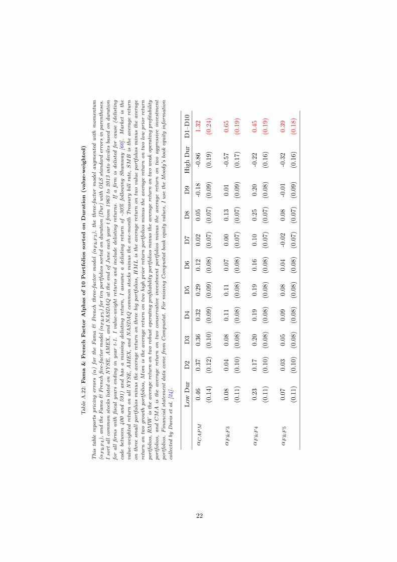
Tab

leA

.22:Fam

a&

French

Facto

rAlp

hasof10

Portfoliosso

rte

don

Duration

(valu

e-w

eighte

d)

Th

ista

ble

repo

rts

pri

cin

ger

rors

(α)

for

the

Fa

ma

&F

ren

chth

ree-

fact

or

mod

el(α

F&F3),

the

thre

e-fa

cto

rm

odel

au

gmen

ted

wit

hm

om

entu

m

(αF&F4),

an

dth

eF

am

a&

Fre

nch

five

-fa

cto

rm

odel

(αF&F5)

for

ten

port

foli

os

sort

edo

nd

ura

tio

n(D

ur)

wit

hO

LS

sta

nd

ard

erro

rsin

pare

nth

eses

.

Iso

rta

llco

mm

on

stoc

ksli

sted

on

NY

SE

,A

ME

X,

an

dN

AS

DA

Qa

tth

een

do

fJ

un

eea

chyea

rt

fro

m1

96

3to

20

13

into

dec

iles

base

do

nd

ura

tio

n

for

all

firm

sw

ith

fisc

al

yea

rsen

din

gin

yea

rt-

1.

Iva

lue-

wei

ght

retu

rns

an

din

clu

de

del

isti

ng

retu

rns.

Ifa

firm

isd

elis

ted

for

cau

se(d

elis

tin

g

cod

ebe

twee

n4

00

an

d5

91

)a

nd

ha

sa

mis

sin

gd

elis

tin

gre

turn

,I

ass

um

ea

del

isti

ng

retu

rno

f-3

0%

foll

ow

ing

Sh

um

wa

y[6

0].

Ma

rket

isth

e

valu

e-w

eigh

ted

retu

rno

na

llN

YS

E,

AM

EX

,a

nd

NA

SD

AQ

com

mo

nst

ocks

min

us

the

on

e-m

on

thT

rea

sury

bill

rate

,SMB

isth

ea

vera

gere

turn

on

thre

esm

all

port

foli

os

min

us

the

ave

rage

retu

rno

nth

ree

big

port

foli

os,HML

isth

ea

vera

gere

turn

on

two

valu

epo

rtfo

lio

sm

inu

sth

ea

vera

ge

retu

rno

ntw

ogr

ow

thpo

rtfo

lio

s,Mom

isth

ea

vera

gere

turn

on

two

hig

hp

rio

rre

turn

port

foli

os

min

us

the

ave

rage

retu

rno

ntw

olo

wp

rio

rre

turn

port

foli

os,RMW

isth

ea

vera

gere

turn

on

two

robu

sto

pera

tin

gp

rofi

tabi

lity

port

foli

os

min

us

the

ave

rage

retu

rno

ntw

ow

eak

ope

rati

ng

pro

fita

bili

ty

port

foli

os,

an

dCMA

isth

ea

vera

gere

turn

on

two

con

serv

ati

vein

vest

men

tpo

rtfo

lio

sm

inu

sth

ea

vera

gere

turn

on

two

agg

ress

ive

inve

stm

ent

port

foli

os.

Fin

an

cia

lst

ate

men

td

ata

com

efr

om

Co

mp

ust

at.

Fo

rm

issi

ng

Co

mp

ust

at

boo

keq

uit

yva

lues

,I

use

the

Moo

dy’s

boo

keq

uit

yin

form

ati

on

coll

ecte

dby

Da

vis

eta

l.[2

4].

Low

Du

rD

2D

3D

4D

5D

6D

7D

8D

9H

igh

Du

rD

1–D

10

αCAPM

0.46

0.37

0.36

0.3

20.2

90.1

20.0

20.0

5-0

.18

-0.8

61.3

2

(0.1

4)(0

.12)

(0.1

0)

(0.0

9)

(0.0

9)

(0.0

8)

(0.0

7)

(0.0

7)

(0.0

9)

(0.1

9)

(0.2

4)

αF&F3

0.08

0.04

0.08

0.1

10.1

10.0

70.0

00.1

30.0

1-0

.57

0.6

5

(0.1

1)(0

.10)

(0.0

8)

(0.0

8)

(0.0

8)

(0.0

8)

(0.0

7)

(0.0

7)

(0.0

9)

(0.1

7)

(0.1

9)

αF&F4

0.23

0.17

0.20

0.1

90.1

90.1

60.1

00.2

50.2

0-0

.22

0.4

5

(0.1

1)(0

.10)

(0.0

8)

(0.0

8)

(0.0

8)

(0.0

8)

(0.0

7)

(0.0

7)

(0.0

8)

(0.1

6)

(0.1

9)

αF&F5

0.07

0.03

0.05

0.0

90.0

80.0

4-0

.02

0.0

8-0

.01

-0.3

20.3

9

(0.1

1)(0

.10)

(0.0

8)

(0.0

8)

(0.0

8)

(0.0

8)

(0.0

7)

(0.0

7)

(0.0

9)

(0.1

6)

(0.1

8)

22

Tab

leA

.23:M

ean

Excess

Retu

rnsof10

Portfoliosso

rte

don

Duration

(robustness,valu

e-w

eighte

d)

Th

ista

ble

repo

rts

mo

nth

lym

ean

exce

ssre

turn

sw

ith

OL

Sst

an

da

rder

rors

inpa

ren

thes

esfo

rva

ria

tio

ns

of

the

para

met

erva

lues

use

dto

calc

ula

te

du

rati

on

inS

ecti

on

2.

Iso

rta

llco

mm

on

stoc

ksli

sted

on

NY

SE

,A

ME

X,

an

dN

AS

DA

Qa

tth

een

do

fJ

un

eea

chyea

rt

fro

m1

96

3to

20

13

into

dec

iles

base

do

nd

ura

tio

nfo

ra

llfi

rms

wit

hfi

sca

lyea

rsen

din

gin

yea

rt-

1.

Iva

lue-

wei

ght

retu

rns

an

din

clu

de

del

isti

ng

retu

rns.

Ifa

firm

isd

elis

ted

for

cau

se

(del

isti

ng

cod

ebe

twee

n4

00

an

d5

91

)a

nd

ha

sa

mis

sin

gd

elis

tin

gre

turn

,I

ass

um

ea

del

isti

ng

retu

rno

f-3

0%

foll

ow

ing

Sh

um

wa

y[6

0].

Fin

an

cia

l

sta

tem

ent

da

taco

me

fro

mC

om

pu

sta

t.F

or

mis

sin

gC

om

pu

sta

tbo

ok

equ

ity

valu

es,

Iu

seth

eM

ood

y’s

boo

keq

uit

yin

form

ati

on

coll

ecte

dby

Da

vis

eta

l.

[24

].

Low

Du

rD

2D

3D

4D

5D

6D

7D

8D

9H

igh

Du

rD

1–D

10

(1)

r=

0.10

1.06

0.87

0.8

60.8

40.7

50.5

80.6

00.5

30.4

2-0

.18

1.2

4

(0.2

4)(0

.22)

(0.2

1)

(0.2

0)

(0.1

9)

(0.1

9)

(0.1

9)

(0.2

0)

(0.2

2)

(0.3

1)

(0.2

4)

(2)

r=

0.14

0.99

0.89

0.8

70.8

10.7

70.6

10.5

40.5

40.3

9-0

.18

1.1

7

(0.2

4)(0

.22)

(0.2

1)

(0.2

0)

(0.1

9)

(0.1

9)

(0.1

9)

(0.1

9)

(0.2

4)

(0.3

2)

(0.2

5)

(3)

ar r

oe

=0.

301.

481.

221.2

01.1

01.0

00.9

70.8

50.7

10.5

70.1

71.3

2

(0.2

6)(0

.24)

(0.2

4)

(0.2

4)

(0.2

4)

(0.2

4)

(0.2

5)

(0.2

6)

(0.2

7)

(0.3

3)

(0.1

9)

(4)

ar r

oe

=0.

501.

471.

231.1

91.0

91.0

10.9

50.8

50.7

20.5

60.1

81.2

9

(0.2

6)(0

.24)

(0.2

4)

(0.2

4)

(0.2

4)

(0.2

4)

(0.2

5)

(0.2

6)

(0.2

7)

(0.3

3)

(0.1

9)

(6)

roe s

s=

0.10

0.93

0.90

0.8

40.8

50.7

10.6

20.5

20.5

10.2

7-0

.21

1.1

4

(0.2

4)(0

.21)

(0.2

1)

(0.2

0)

(0.1

9)

(0.1

9)

(0.1

9)

(0.2

0)

(0.2

8)

(0.3

2)

(0.2

5)

(5)

roe s

s=

0.14

1.07

0.87

0.8

50.8

10.7

10.6

00.6

30.5

10.4

3-0

.07

1.1

4

(0.2

4)(0

.23)

(0.2

1)

(0.2

0)

(0.1

9)

(0.1

9)

(0.1

9)

(0.1

9)

(0.2

1)

(0.3

1)

(0.2

3)

(9)

ar s

g=

0.20

1.00

0.88

0.8

30.7

90.7

40.6

10.5

70.5

40.3

9-0

.15

1.1

5

(0.2

4)(0

.22)

(0.2

1)

(0.2

0)

(0.1

9)

(0.1

9)

(0.1

9)

(0.2

0)

(0.2

2)

(0.3

2)

(0.2

4)

(10)

ar s

g=

0.30

1.06

0.87

0.8

50.8

40.7

50.6

20.5

40.5

40.3

8-0

.17

1.2

3

(0.2

4)(0

.22)

(0.2

1)

(0.2

0)

(0.1

9)

(0.1

9)

(0.1

9)

(0.1

9)

(0.2

3)

(0.3

2)

(0.2

5)

(7)

sgss

=0.

080.

960.

880.8

70.8

40.6

90.6

60.5

20.5

00.3

2-0

.23

1.1

9

(0.2

4)(0

.21)

(0.2

1)

(0.2

0)

(0.1

9)

(0.1

9)

(0.1

9)

(0.2

0)

(0.2

7)

(0.3

2)

(0.2

4)

(8)

sgss

=0.

041.

070.

870.8

30.8

10.7

40.5

90.6

10.5

40.4

1-0

.12

1.1

9

(0.2

4)(0

.22)

(0.2

1)

(0.2

0)

(0.1

9)

(0.1

9)

(0.2

0)

(0.1

9)

(0.2

1)

(0.3

2)

(0.2

4)

(11)

horizon

=10

0.97

0.88

0.8

80.8

40.7

10.6

60.5

30.5

10.3

3-0

.22

1.1

8

(0.2

4)(0

.22)

(0.2

1)

(0.2

0)

(0.1

9)

(0.1

9)

(0.1

9)

(0.2

0)

(0.2

6)

(0.3

2)

(0.2

4)

23

Tab

leA

.24:M

ean

Excess

Retu

rnsof10

Portfoliosso

rte

don

Duration

(subsa

mples,

valu

e-w

eighte

d)

Th

ista

ble

repo

rts

mo

nth

lym

ean

exce

ssre

turn

sw

ith

OL

Sst

an

da

rder

rors

inpa

ren

thes

esfo

rd

iffer

ent

subs

am

ple

s.I

sort

all

com

mo

nst

ocks

list

ed

on

NY

SE

,A

ME

X,

an

dN

AS

DA

Qa

tth

een

do

fJ

un

eea

chyea

rt

fro

m1

96

3to

20

13

into

dec

iles

base

do

nd

ura

tio

nfo

ra

llfi

rms

wit

hfi

sca

lyea

rs

end

ing

inyea

rt-

1.

Iva

lue-

wei

ght

retu

rns

an

din

clu

de

del

isti

ng

retu

rns.

Ifa

firm

isd

elis

ted

for

cau

se(d

elis

tin

gco

de

betw

een

40

0a

nd

59

1)

an

dh

as

a

mis

sin

gd

elis

tin

gre

turn

,I

ass

um

ea

del

isti

ng

retu

rno

f-3

0%

foll

ow

ing

Sh

um

wa

y[6

0].

Fin

an

cia

lst

ate

men

td

ata

com

efr

om

Co

mp

ust

at.

Fo

rm

issi

ng

Co

mp

ust

at

boo

keq

uit

yva

lues

,I

use

the

Moo

dy’s

boo

keq

uit

yin

form

ati

on

coll

ecte

dby

Da

vis

eta

l.[2

4].

Low

Du

rD

2D

3D

4D

5D

6D

7D

8D

9H

igh

Du

rD

1–D

10

PanelA.July

1963–June1973

Mea

n0.

390.

520.

44

0.5

80.5

4-0

.03

-0.1

40.0

80.2

20.4

5-0

.06

SE

(0.4

6)(0

.44)

(0.3

9)

(0.4

0)

(0.3

7)

(0.3

6)

(0.3

9)

(0.3

8)

(0.4

2)

(0.3

8)

(0.3

4)

PanelB.July

1973–June1983

Mea

n1.

171.

231.

08

1.0

10.6

80.7

90.6

30.5

80.3

0-0

.27

1.4

4

SE

(0.6

2)(0

.55)

(0.5

3)

(0.5

1)

(0.4

7)

(0.4

7)

(0.4

9)

(0.5

0)

(0.5

3)

(0.6

0)

(0.5

0)

PanelC.July

1983–June1993

Mea

n1.

260.

930.

87

0.8

30.5

30.7

30.5

80.5

50.3

3-0

.62

1.8

8

SE

(0.4

9)(0

.44)

(0.4

7)

(0.4

6)

(0.4

3)

(0.4

7)

(0.4

5)

(0.4

7)

(0.5

4)

(0.6

7)

(0.4

9)

PanelD.July

1993–June2003

Mea

n0.

820.

700.

74

0.7

10.9

70.6

60.7

70.7

00.5

0-1

.04

1.8

6

SE

(0.5

1)(0

.54)

(0.4

7)

(0.4

5)

(0.4

4)

(0.4

6)

(0.4

6)

(0.4

4)

(0.6

0)

(1.1

0)

(0.8

5)

PanelE.July

2003–June2014

Mea

n1.

361.

051.

17

0.9

71.0

80.8

30.8

10.8

10.5

90.6

80.6

7

SE

(0.5

7)(0

.50)

(0.4

6)

(0.4

2)

(0.4

3)

(0.3

5)

(0.3

8)

(0.3

7)

(0.4

2)

(0.6

1)

(0.3

9)

24

Tab

leA

.25:M

ean

Retu

rnsand

Alp

hasof10

Portfoliosso

rte

don

Duration:Volatility

-managed

Portfolios(v

alu

e-w

eighte

d)

Th

ista

ble

repo

rts

mea

nre

turn

sa

nd

pri

cin

ger

rors

(α)

for

the

CA

PM

(αCAPM

),th

eF

am

a&

Fre

nch

thre

e-fa

cto

rm

odel

(αF&F3),

the

thre

e-fa

cto

r

mod

ela

ugm

ente

dw

ith

mo

men

tum

(αF&F4),

an

dth

eF

am

a&

Fre

nch

five

-fa

cto

rm

odel

(αF&F5)

for

ten

port

foli

os

sort

edo

nd

ura

tio

n(D

ur)

wit

h

OL

Sst

an

da

rder

rors

inpa

ren

thes

es.

Po

rtfo

lio

retu

rns

are

sca

led

byth

ep

revi

ou

sm

on

ths

rea

lize

dva

ria

nce

as

inM

ore

ira

an

dM

uir

[54

].I

sort

all

com

mo

nst

ocks

list

edo

nN

YS

E,

AM

EX

,a

nd

NA

SD

AQ

at

the

end

of

Ju

ne

each

yea

rt

fro

m1

96

3to

20

13

into

dec

iles

base

do

nd

ura

tio

nfo

ra

ll

firm

sw

ith

fisc

al

yea

rsen

din

gin

yea

rt-

1.

Iva

lue-

wei

ght

retu

rns

an

din

clu

de

del

isti

ng

retu

rns.

Ifa

firm

isd

elis

ted

for

cau

se(d

elis

tin

gco

de

betw

een

40

0a

nd

59

1)

an

dh

as

am

issi

ng

del

isti

ng

retu

rn,

Ia

ssu

me

ad

elis

tin

gre

turn

of

-30

%fo

llo

win

gS

hu

mw

ay

[60

].M

ark

etis

the

valu

e-w

eigh

ted

retu

rn

on

all

NY

SE

,A

ME

X,

an

dN

AS

DA

Qco

mm

on

stoc

ksm

inu

sth

eo

ne-

mo

nth

Tre

asu

rybi

llra

te,SMB

isth

ea

vera

gere

turn

on

thre

esm

all

port

foli

os

min

us

the

ave

rage

retu

rno

nth

ree

big

port

foli

os,HML

isth

ea

vera

gere

turn

on

two

valu

epo

rtfo

lio

sm

inu

sth

ea

vera

gere

turn

on

two

gro

wth

port

foli

os,Mom

isth

ea

vera

gere

turn

on

two

hig

hp

rio

rre

turn

port

foli

os

min

us

the

ave

rage

retu

rno

ntw

olo

wp

rio

rre

turn

port

foli

os,RMW

isth

ea

vera

gere

turn

on

two

robu

sto

pera

tin

gp

rofi

tabi

lity

port

foli

os

min

us

the

ave

rage

retu

rno

ntw

ow

eak

ope

rati

ng

pro

fita

bili

typo

rtfo

lio

s,a

nd

CMA

isth

ea

vera

gere

turn

on

two

con

serv

ati

vein

vest

men

tpo

rtfo

lio

sm

inu

sth

ea

vera

gere

turn

on

two

agg

ress

ive

inve

stm

ent

port

foli

os.

Fin

an

cia

l

sta

tem

ent

da

taco

me

fro

mC

om

pu

sta

t.F

or

mis

sin

gC

om

pu

sta

tbo

ok

equ

ity

valu

es,

Iu

seth

eM

ood

y’s

boo

keq

uit

yin

form

ati

on

coll

ecte

dby

Da

vis

eta

l.[2

4].

Low

Du

rD

2D

3D

4D

5D

6D

7D

8D

9H

igh

Du

rD

1–D

10

Mea

n1.

361.

201.

17

1.1

61.1

11.0

30.8

90.8

70.7

30.5

21.3

1

SE

(0.2

4)(0

.22)

(0.2

1)

(0.2

0)

(0.1

9)

(0.1

9)

(0.2

0)

(0.1

9)

(0.2

3)

(0.3

2)

(0.2

4)

αCAPM

0.96

0.83

0.81

0.8

20.7

80.7

00.5

50.5

20.3

5-0

.04

1.4

0

SE

(0.1

9)(0

.18)

(0.1

6)

(0.1

6)

(0.1

5)

(0.1

5)

(0.1

5)

(0.1

5)

(0.1

8)

(0.2

5)

(0.2

4)

αF&F3

0.80

0.70

0.69

0.7

50.7

30.7

00.5

60.6

10.4

60.1

40.9

6

SE

(0.1

9)(0

.18)

(0.1

6)

(0.1

6)

(0.1

5)

(0.1

5)

(0.1

5)

(0.1

5)

(0.1

8)

(0.2

4)

(0.2

2)

αF&F4

0.75

0.65

0.61

0.6

40.6

20.6

10.4

50.5

10.3

60.0

80.8

5

SE

(0.2

0)(0

.18)

(0.1

7)

(0.1

7)

(0.1

6)

(0.1

5)

(0.1

6)

(0.1

5)

(0.1

9)

(0.2

5)

(0.2

3)

αF&F5

0.66

0.61

0.59

0.6

30.6

30.6

00.4

10.4

10.3

10.0

40.8

3

SE

(0.2

0)(0

.18)

(0.1

7)

(0.1

7)

(0.1

6)

(0.1

5)

(0.1

6)

(0.1

5)

(0.1

9)

(0.2

5)

(0.2

3)

25

Tab

leA

.26:Fam

a&

French

Alp

hasof10

Portfoliosso

rte

don

Duration

Conditionalon

InvestorSentim

ent(v

alu

e-w

eighte

d)

Th

ista

ble

repo

rts

ben

chm

ark

-ad

just

edm

ean

exce

ssre

turn

sfo

llo

win

gpe

riod

so

fh

igh

an

dlo

win

vest

or

sen

tim

ent

inP

an

elA

,a

sw

ell

as

sen

tim

ent

beta

s

inP

an

elB

for

ten

port

foli

os

sort

edo

nd

ura

tio

n(D

ur)

wit

hO

LS

sta

nd

ard

erro

rsin

pare

nth

eses

.I

sort

all

com

mo

nst

ocks

list

edo

nN

YS

E,

AM

EX

,a

nd

NA

SD

AQ

at

the

end

of

Ju

ne

each

yea

rt

fro

m1

96

3to

20

13

into

dec

iles

base

do

nd

ura

tio

nfo

ra

llfi

rms

wit

hfi

sca

lyea

rsen

din

gin

yea

rt-

1.

Iva

lue-

wei

ght

retu

rns

an

din

clu

de

del

isti

ng

retu

rns.

Ifa

firm

isd

elis

ted

for

cau

se(d

elis

tin

gco

de

betw

een

40

0a

nd

59

1)

an

dh

as

am

issi

ng

del

isti

ng

retu

rn,

Ia

ssu

me

a

del

isti

ng

retu

rno

f-3

0%

foll

ow

ing

Sh

um

wa

y[6

0].

Id

efin

eh

igh

an

dlo

wse

nti

men

tpe

riod

sby

the

mea

nle

vel

of

the

sen

tim

ent

ind

exo

fB

ake

ra

nd

Wu

rgle

r

[7].

Sen

tim

ent

beta

sa

reth

eti

me

seri

esfa

cto

rlo

ad

ings

of

the

ben

chm

ark

-ad

just

edm

ean

exce

ssre

turn

so

na

con

sta

nt

an

dch

an

ges

inth

ese

nti

men

tin

dex

.

Fin

an

cia

lst

ate

men

td

ata

com

efr

om

Co

mp

ust

at.

Fo

rm

issi

ng

Co

mp

ust

at

boo

keq

uit

yva

lues

,I

use

the

Moo

dy’s

boo

keq

uit

yin

form

ati

on

coll

ecte

dby

Da

vis

eta

l.[2

4].

Iu

seth

eF

am

a&

Fre

nch

thre

e-fa

cto

rm

odel

as

ben

chm

ark

.T

he

sam

ple

peri

odis

Ju

ly1

96

5to

Dec

embe

r2

01

0d

ue

toth

ea

vail

abi

lity

of

the

sen

tim

ent

ind

ex.

Low

Du

rD

2D

3D

4D

5D

6D

7D

8D

9H

igh

Du

rD

1–D

10

PanelA.SentimentAlphas

αH

ighSent

-0.0

40.

020.0

00.1

80.1

90.1

70.0

50.0

8-0

.20

-1.3

31.2

9

(0.1

7)(0

.16)

(0.1

3)

(0.1

2)

(0.1

2)

(0.1

2)

(0.1

0)

(0.1

0)

(0.1

3)

(0.2

6)

(0.2

9)

αLowSent

0.11

0.09

0.1

50.0

90.0

4-0

.03

-0.0

80.2

20.2

00.0

40.0

7

(0.1

6)(0

.15)

(0.1

2)

(0.1

2)

(0.1

2)

(0.1

2)

(0.1

0)

(0.1

0)

(0.1

3)

(0.2

5)

(0.2

8)

PanelB.SentimentBeta

s

βSent

1.38

1.13

0.9

51.0

60.7

20.8

51.0

61.1

01.5

32.7

6-1

.38

(0.2

5)(0

.24)

(0.2

2)

(0.2

1)

(0.2

1)

(0.2

0)

(0.2

1)

(0.2

1)

(0.2

4)

(0.3

3)

(0.2

6)

26

Table A.27: Mean Excess Returns of 25 Portfolios sorted on Duration and Residual Institutional Ownership(value-weighted)

This table reports monthly mean excess returns for twenty-five portfolios sorted on duration (Dur)

and residual institutional ownership (RIOR) with OLS standard errors in parentheses. I sort

all common stocks listed on NYSE, AMEX, and NASDAQ at the end of June each year t from

1981 to 2013 into quintiles based on duration for all firms with fiscal years ending in year t-1.

I intersect these quintiles with an independent sort on residual institutional ownership as of

December t-1. I value-weight returns and include delisting returns. If a firm is delisted for cause

(delisting code between 400 and 591) and has a missing delisting return, I assume a delisting

return of -30% following Shumway [60]. Dur is cash flow duration. RIOR is the residual in

a cross sectional regression of the fraction of shares held by institutions on size. Institutional

ownership information is obtained from the Thomson Reuters 13F database. Financial statement

data come from Compustat. For missing Compustat book equity values, I use the Moody’s book

equity information collected by Davis et al. [24]. I only use stocks above the 20th size percentile.

Low Dur D2 D3 D4 High Dur D1–D5

Mea

n

Low RIOR 1.11 0.80 0.71 0.65 0.13 0.98

(0.32) (0.26) (0.28) (0.29) (0.42) (0.31)

RIOR2 0.95 0.92 0.84 0.79 0.44 0.52

(0.29) (0.26) (0.26) (0.24) (0.31) (0.25)

RIOR3 0.99 0.80 0.85 0.63 0.30 0.69

(0.28) (0.27) (0.25) (0.26) (0.31) (0.24)

RIOR4 0.77 0.89 0.60 0.56 0.41 0.36

(0.28) (0.27) (0.26) (0.27) (0.37) (0.31)

High RIOR 1.06 0.87 0.89 0.67 0.58 0.48

(0.31) (0.29) (0.29) (0.33) (0.39) (0.29)

RIOR1 – RIOR5 0.06 -0.08 -0.18 -0.02 -0.45 0.50

(0.26) (0.19) (0.24) (0.24) (0.27) (0.35)

27

Table A.28: CAPM Alphas 25 Portfolios sorted on Duration and Residual Institutional Ownership (value-weighted)

This table reports pricing errors (α) for the CAPM for twenty-five portfolios sorted on duration

(Dur) and residual institutional ownership (RIOR) with OLS standard errors in parentheses. I sort

all common stocks listed on NYSE, AMEX, and NASDAQ at the end of June each year t from

1981 to 2013 into quintiles based on duration for all firms with fiscal years ending in year t-1. I

intersect these quintiles with an independent sort on residual institutional ownership as of December

t-1. I value-weight returns and include delisting returns. If a firm is delisted for cause (delisting

code between 400 and 591) and has a missing delisting return, I assume a delisting return of -30%

following Shumway [60]. Market is the value weighted return on all NYSE, AMEX, and NASDAQ

common stocks minus the one-month Treasury bill rate, SMB is the average return on three small

portfolios minus the average return on three big portfolios, and HML is the average return on two

value portfolios minus the average return on two growth portfolios. Dur is cash flow duration. RIOR

is the residual in a cross sectional regression of the fraction of shares held by institutions on size.

Institutional ownership information is obtained from the Thomson Reuters 13F database. Financial

statement data come from Compustat. For missing Compustat book equity values, I use the Moody’s

book equity information collected by Davis et al. [24]. I only use stocks above the 20th size percentile.

Low Dur D2 D3 D4 High Dur D1–D5

αCAPM

Low RIOR 0.46 0.17 0.06 -0.05 -0.83 1.29

(0.23) (0.14) (0.15) (0.14) (0.24) (0.29)

RIOR2 0.31 0.28 0.18 0.17 -0.32 0.62

(0.17) (0.13) (0.12) (0.10) (0.16) (0.25)

RIOR3 0.34 0.16 0.24 -0.05 -0.43 0.77

(0.16) (0.15) (0.13) (0.10) (0.18) (0.24)

RIOR4 0.13 0.26 -0.02 -0.11 -0.40 0.52

(0.17) (0.15) (0.15) (0.14) (0.24) (0.31)

High RIOR 0.36 0.19 0.27 -0.05 -0.32 0.67

(0.18) (0.16) (0.19) (0.21) (0.23) (0.29)

RIOR1 – RIOR5 0.11 -0.02 -0.21 0.00 -0.51 0.62

(0.26) (0.19) (0.25) (0.25) (0.27) (0.35)

28

Table A.29: Fama - French Alphas of 25 Portfolios sorted on Duration and Residual Institutional Ownership(value-weighted)

This table reports pricing errors (α) for the Fama & French three-factor model for twenty-five

portfolios sorted on duration (Dur) and residual institutional ownership (RIOR) with OLS standard

errors in parentheses. I sort all common stocks listed on NYSE, AMEX, and NASDAQ at the end

of June each year t from 1981 to 2013 into quintiles based on duration for all firms with fiscal years

ending in year t-1. I intersect these quintiles with an independent sort on residual institutional

ownership as of December t-1. I value-weight returns and include delisting returns. If a firm is

delisted for cause (delisting code between 400 and 591) and has a missing delisting return, I assume

a delisting return of -30% following Shumway [60]. Market is the value weighted return on all

NYSE, AMEX, and NASDAQ common stocks minus the one-month Treasury bill rate, SMB is the

average return on three small portfolios minus the average return on three big portfolios, HML is the

average return on two value portfolios minus the average return on two growth portfolios, and Mom

is the average return on two high prior return portfolios minus the average return on two low prior

return portfolios. Dur is cash flow duration. RIOR is the residual in a cross-sectional regression of

the fraction of shares held by institutions on size. Institutional ownership information is obtained

from the Thomson Reuters 13F database. Financial statement data come from Compustat. For

missing Compustat book equity values, I use the Moody’s book equity information collected by Davis

et al. [24]. I only use stocks above the 20th size percentile.

Low Dur D2 D3 D4 High Dur D1–D5

αF&F

Low RIOR 0.25 0.02 -0.08 -0.08 -0.60 0.85

(0.22) (0.14) (0.15) (0.14) (0.23) (0.26)

RIOR2 -0.01 0.09 0.08 0.23 -0.10 0.09

(0.15) (0.12) (0.12) (0.09) (0.14) (0.19)

RIOR3 0.07 -0.11 0.14 0.05 -0.23 0.30

(0.14) (0.13) (0.12) (0.09) (0.17) (0.20)

RIOR4 -0.11 0.07 -0.07 0.01 -0.02 -0.08

(0.15) (0.14) (0.15) (0.13) (0.21) (0.25)

High RIOR -0.01 0.04 0.18 0.11 -0.10 0.09

(0.14) (0.14) (0.18) (0.20) (0.21) (0.23)

RIOR1 – RIOR5 0.26 -0.02 -0.27 -0.19 -0.50 0.76

(0.25) (0.19) (0.24) (0.24) (0.27) (0.36)

29

Table A.30: Four Factor Alphas of 25 Portfolios sorted on Duration and Residual Institutional Ownership(value-weighted)

This table reports pricing errors (α) for Fama & French three-factor model augmented with

momentum for twenty-five portfolios sorted on duration (Dur) and residual institutional ownership

(RIOR) with OLS standard errors in parentheses. I sort all common stocks listed on NYSE, AMEX,

and NASDAQ at the end of June each year t from 1981 to 2013 into quintiles based on duration

for all firms with fiscal years ending in year t-1. I intersect these quintiles with an independent

sort on residual institutional ownership as of December t-1. I v value-weight returns and include

delisting returns. If a firm is delisted for cause (delisting code between 400 and 591) and has a

missing delisting return, I assume a delisting return of -30% following Shumway [60]. Market is the

value-weighted return on all NYSE, AMEX, and NASDAQ common stocks minus the one-month

Treasury bill rate, SMB is the average return on three small portfolios minus the average return

on three big portfolios, HML is the average return on two value portfolios minus the average

return on two growth portfolios, RMW is the average return on two robust operating profitability

portfolios minus the average return on two weak operating profitability portfolios, and CMA is the

average return on two conservative investment portfolios minus the average return on two aggressive

investment portfolios. Dur is cash flow duration. RIOR is the residual in a cross sectional regression

of the fraction of shares held by institutions on size. Institutional ownership information is obtained

from the Thomson Reuters 13F database. Financial statement data come from Compustat. For

missing Compustat book equity values, I use the Moody’s book equity information collected by Davis

et al. [24]. I only use stocks above the 20th size percentile.

Low Dur D2 D3 D4 High Dur D1–D5

α4Factor

Low RIOR 0.51 0.17 0.14 0.13 -0.09 0.60

(0.22) (0.13) (0.14) (0.14) (0.19) (0.26)

RIOR2 0.19 0.24 0.26 0.28 0.12 0.08

(0.14) (0.12) (0.11) (0.10) (0.13) (0.20)

RIOR3 0.24 0.00 0.22 0.19 0.04 0.20

(0.14) (0.13) (0.12) (0.09) (0.16) (0.21)

RIOR4 0.02 0.10 0.06 0.07 0.17 -0.15

(0.15) (0.14) (0.15) (0.13) (0.21) (0.26)

High RIOR 0.22 0.13 0.23 0.31 0.13 0.09

(0.12) (0.15) (0.19) (0.20) (0.21) (0.24)

RIOR1 – RIOR5 0.29 0.04 -0.09 -0.18 -0.22 0.51

(0.25) (0.19) (0.24) (0.24) (0.27) (0.36)

30

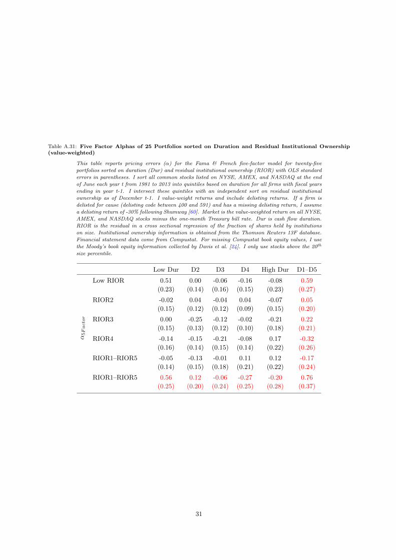
Table A.31: Five Factor Alphas of 25 Portfolios sorted on Duration and Residual Institutional Ownership(value-weighted)

This table reports pricing errors (α) for the Fama & French five-factor model for twenty-five

portfolios sorted on duration (Dur) and residual institutional ownership (RIOR) with OLS standard

errors in parentheses. I sort all common stocks listed on NYSE, AMEX, and NASDAQ at the end

of June each year t from 1981 to 2013 into quintiles based on duration for all firms with fiscal years

ending in year t-1. I intersect these quintiles with an independent sort on residual institutional

ownership as of December t-1. I value-weight returns and include delisting returns. If a firm is

delisted for cause (delisting code between 400 and 591) and has a missing delisting return, I assume

a delisting return of -30% following Shumway [60]. Market is the value-weighted return on all NYSE,

AMEX, and NASDAQ stocks minus the one-month Treasury bill rate. Dur is cash flow duration.

RIOR is the residual in a cross sectional regression of the fraction of shares held by institutions

on size. Institutional ownership information is obtained from the Thomson Reuters 13F database.

Financial statement data come from Compustat. For missing Compustat book equity values, I use

the Moody’s book equity information collected by Davis et al. [24]. I only use stocks above the 20th

size percentile.

Low Dur D2 D3 D4 High Dur D1–D5

α5Factor

Low RIOR 0.51 0.00 -0.06 -0.16 -0.08 0.59

(0.23) (0.14) (0.16) (0.15) (0.23) (0.27)

RIOR2 -0.02 0.04 -0.04 0.04 -0.07 0.05

(0.15) (0.12) (0.12) (0.09) (0.15) (0.20)

RIOR3 0.00 -0.25 -0.12 -0.02 -0.21 0.22

(0.15) (0.13) (0.12) (0.10) (0.18) (0.21)

RIOR4 -0.14 -0.15 -0.21 -0.08 0.17 -0.32

(0.16) (0.14) (0.15) (0.14) (0.22) (0.26)

RIOR1–RIOR5 -0.05 -0.13 -0.01 0.11 0.12 -0.17

(0.14) (0.15) (0.18) (0.21) (0.22) (0.24)

RIOR1–RIOR5 0.56 0.12 -0.06 -0.27 -0.20 0.76

(0.25) (0.20) (0.24) (0.25) (0.28) (0.37)

31