cassini iss observation of saturn•s north polar vortex...
TRANSCRIPT

Icarus 285 (2017) 68–82
Contents lists available at ScienceDirect
Icarus
journal homepage: www.elsevier.com/locate/icarus
Cassini ISS observation of Saturn’s north polar vortex and comparison
to the south polar vortex
Kunio M. Sayanagi a , ∗, John J. Blalock
a , Ulyana A. Dyudina
b , Shawn P. Ewald
b , Andrew P. Ingersoll b
a Department of Atmospheric and Planetary Sciences, Hampton University, Hampton, VA, 23668, USA b Division of Geological and Planetary Sciences, California Institute of Technology, Pasadena, CA, 91125, USA
a r t i c l e i n f o
Article history:
Received 16 February 2016
Revised 1 December 2016
Accepted 5 December 2016
Available online 13 December 2016
Keywords:
Atmospheres, dynamics
Saturn, atmosphere
Jovian planets
Saturn
a b s t r a c t
We present analyses of Saturn’s north pole using high-resolution images captured in late 2012 by the
Cassini spacecraft’s Imaging Science Subsystem (ISS) camera. The images reveal the presence of an intense
cyclonic vortex centered at the north pole. In the red and green visible continuum wavelengths, the north
polar region exhibits a cyclonically spiraling cloud morphology extending from the pole to 85 °N plane-
tocentric latitude, with a 4700 km radius. Images captured in the methane bands, which sense upper
tropospheric haze, show an approximately circular hole in the haze extending up to 1.5 ° latitude away
from the pole. The spiraling morphology and the “eye”-like hole at the center are reminiscent of a terres-
trial tropical cyclone. In the System III reference frame (rotation period of 10h39m22.4s, Seidelmann et al.
2007; Archinal et al. 2011), the eastward wind speed increases to about 140 m s −1 at 89 °N planetocentric
latitude. The vorticity is (6.5 ± 1.5) ×10 −4 s −1 at the pole, and decreases to (1.3 ± 1.2) ×10 −4 s −1 at 89 °N.
In addition, we present an analysis of Saturn’s south polar vortex using images captured in January 2007
to compare its cloud morphology to the north pole. The set of images captured in 2007 includes filters
that have not been analyzed before. Images captured in the violet filter (400 nm) also reveal a bright po-
lar cloud. The south polar morphology in 2007 was more smooth and lacked the small clouds apparent
around the north pole in 2012. Saturn underwent equinox in August 2009. The 2007 observation cap-
tured the pre-equinox south pole, and the 2012 observation captured the post-equinox north pole. Thus,
the observed differences between the poles are likely due to seasonal effects. If these differences indeed
are caused by seasonal effects, continuing observations of the summer north pole by the Cassini mission
should show a formation of a polar cloud that appears bright in short-wavelength filters.
© 2016 Elsevier Inc. All rights reserved.
t
w
l
p
e
p
C
5
b
t
1. Introduction
On November 27, 2012, Cassini orbiter’s Imaging Science Sub-
system (ISS) camera returned high-resolution images of the north
pole of Saturn illuminated by sunlight for the first time since the
equinox in 1994. Before 1994, the northern high-latitudes were
imaged by Voyager 1 & 2 in 1980–1981 ( Godfrey, 1988 ), by the
Hubble Space Telescope in 1990 ( Caldwell et al., 1993 ), and by
ground-based telescopes ( Sanchez-Lavega et al., 1993; 1997 ). How-
ever, these images captured before the 1994 equinox did not re-
solve the north pole due to low image resolution and observation
geometry that had severe foreshortening of the north pole.
∗ Corresponding author.
E-mail addresses: [email protected] , [email protected]
(K.M. Sayanagi).
e
n
t
o
e
http://dx.doi.org/10.1016/j.icarus.2016.12.011
0019-1035/© 2016 Elsevier Inc. All rights reserved.
When Cassini spacecraft entered orbit around Saturn in 2004,
he northern high-latitudes were in winter polar night, and ISS,
hich senses scattered sunlight in visible and near-infrared wave-
engths, was not able to image the pole. Prior to the present re-
ort, the Cassini Composite Infrared Spectrometer (CIRS) ( Fletcher
t al., 2008 ) observed thermal emissions from the polar region, and
redicted cyclonic vorticity at the north pole. Observation by the
assini Visible and Infrared Mapping Spectrometer (VIMS), whose
- μ m images reveal the motion of clouds silhouetted against the
ackground thermal emissions, confirmed the strong cyclonic mo-
ion at the pole ( Baines et al., 2009 ).
Sunlight started shining on the north pole of Saturn after the
quinox in August 2009; however, Cassini had a poor view of the
orth pole until late 2012 because the orbiter stayed in an equa-
orial orbit. Using the 2012 data, we report the cloud morphol-
gy and wind field of Saturn’s North Polar Vortex (NPV). Antuñano
t al. (2015) previously measured the wind structure around both

K.M. Sayanagi et al. / Icarus 285 (2017) 68–82 69
Table 1
When a range is given, the first number corresponds to that at the beginning of the imaging sequence, and the second to
the value at the end of the sequence.
Camera Year-Month-Day Distance from Saturn a Sub-spacecraft latitude Solar phase angle Pixel scale
NAC 2012-11-27 418,142 –457,351 km 37 .9 °N–46.3 °N 93 .5 °–65.9 ° 2 km
WAC 2012-12-10 448,523 –533,304 km 37 .0 °N–51.8 °N 105 .8 °–62.5 ° 23–28 km
NAC 2008-07-14 333,218 –390,607 km 64 .8 °S–56.6 °S 67 .1 °–57.4 ° 2 km
WAC 2007-01-30 1,029,965 –1,014,265 km 35 .8 °S–39.3 °S 120 .5 °–102.6 ° 60 km
a Distance is measured from the center of Saturn.
o
r
r
l
s
(
s
i
S
e
2
p
e
C
s
J
T
p
t
(
D
e
–
p
v
c
u
e
g
C
(
i
(
u
r
t
o
u
p
s
0
a
3
3
8
F
F
fi
s
t
a
R
F
b
m
8
m
n
d
f
h
h
s
a
t
M
p
i
s
a
t
h
T
r
o
d
e
o
t
a
6
1
p
a
f
V
C
w
i
t
n
i
r
d
i
a
i
m
a
e
d
f the poles; our current wind measurements focus on a smaller
egion immediately around the north pole with a higher spatial
esolution, and we also analyze the morphology in multiple wave-
engths using different ISS filters. These images also captured the
urrounding hexagonal jet pattern originally discovered by Godfrey
1988) ; our analysis of the hexagon will be reported separately.
The rest of our report is organized as follows. Section 2 de-
cribes the ISS image sets and the processing applied to them
n our study. Section 3 presents our measurements of the NPV.
ection 4 compares the NPV to the South Polar Vortex observed
arlier in the Cassini mission. Section 5 summarizes our results.
. ISS image sets
We analyze both the north and south poles of Saturn in this re-
ort. To study the north pole, we analyze the Narrow-Angle Cam-
ra (NAC) images captured on November 27, 2012 and Wide-Angle
amera (WAC) images captured on December 10, 2012. For the
outh polar analysis, we examine WAC images captured between
anuary 30–31, 2007, and NAC images captured on July 14, 2008.
he imaging observation geometries of those image sequences are
resented in Table 1 . Previously, NAC images of the south pole cap-
ured in July–August 2004 were presented by Sánchez-Lavega et al.
2006) and those captured on October 11, 2006 were presented by
yudina et al. (20 08, 20 09) and Antuñano et al. (2015) . Antuñano
t al. (2015) also analyzed CB2 and CB3 images captured in June
December 2013 of the north polar region. Our current report
resents images captured using filters not included in these pre-
ious studies and/or in higher spatial resolution.
We follow the standard image calibration and processing pro-
edure previously used by others to process ISS images of Sat-
rn, e.g., Porco et al. (2005) , Vasavada et al. (2006) , Del Genio
t al. (2007) , and Sayanagi et al. (2013, 2014) . We use the camera
eometric model and the photometric calibration software CISS-
AL version 3.4 described by Porco et al. (2004) and West et al.
2010) and released on April 9, 2006. The photometric flatten-
ng and mosaicing procedures are the same as in Sayanagi et al.
2013, 2014) . Image navigation and map projection procedures
sed the equatorial and polar radii of 60,268 km and 54,364 km,
espectively ( Lindal et al., 1985 ). We use the System III longi-
ude (rotation rate of � = 1.638 ×10 −4 s −1 , and rotation period
f 10h39m22.4s; Seidelmann et al. 2007; Archinal et al. 2011 ). We
se the planetocentric latitude throughout our report. We map the
hotometrically flattened images in polar orthographic projection
uch that our polar maps, centered on the pole, are re-sampled to
.07 ° and 0.0028 ° of latitude per pixel for the WAC and NAC im-
ges, respectively.
. Analysis
.1. Cloud morphology
Figs. 1 and 2 show the morphological context poleward of
3 °N that surrounds the polar vortex captured in the WAC images.
ig. 1 depicts the morphology captured in individual filters, and
ig. 2 presents color composites that combine views of multiple
lters. Images captured in CB2 filter (757 nm continuum, Fig. 1 a)
how a spiraling cloud morphology poleward of 85 °N. The sense of
he spiral is cyclonic, i.e., the spiral arms turn counter-clockwise
s they move away from the center. The NPV’s appearances in
ED (648 nm broadband, Fig. 1 e) and GRN (567 nm broadband,
ig. 1 f) filters are similar to that in CB2. In BL1 (460 nm broad-
and, Fig. 1 g), and VIO (420 nm broadband, Fig. 1h), the spiraling
orphology is barely discernible, and latitudes poleward of about
9.5 °N are dark, appearing as a circular hole. In MT2 (728 nm
oderate methane absorption band, Fig. 1 c), the contrast is domi-
ated by the dark circular hole centered on the pole and extending
own to 88.5 °N. The outline of the circular hole is sharp as will be
urther illustrated using the NAC images. In the MT2 view, the dark
ole is surrounded by a gradual darkening toward the edge of the
ole — the darkening becomes discernible poleward of 86.5 °N. The
ame hole can be found in the MT3 view (889 nm strong methane
bsorption band, Fig. 1 d); however, the contrast is much weaker
han in MT2. We interpret the dark appearance of the pole in MT2,
T3, BL1 and VIO as a lack of reflecting aerosols rather than a
resence of dark aerosols because no such darkening can be seen
n CB2 and CB3. We also note that the size of this hole appears
maller in BL1 and VIO than in MT2 and MT3; since the methane
bsorption band filters MT2 and MT3 sense higher altitudes than
he broad band visible filters BL1 and VIO, we interpret that the
ole is larger in the upper altitudes sensed by the methane filters.
he uniform scattering of shorter wavelengths BL1 and VIO in the
egion outside the hole is also indicative of the presence of a layer
f single-scattering particles smaller than ∼ 400 nm. Quantitative
etermination of the cloud and haze layer altitudes would require
xtensive radiative transfer modeling, which is beyond the scope
f our study; García-Melendo et al. (2009, 2011) estimated that
he CB2 filter senses altitudes between 350 mbar and 700 mbar,
nd MT2 and MT3 are sensitive to a range between 250 mbar and
0 mbar.
In Fig. 1 d (MT3) and 1h (VIO), 29 and 30 images captured over
1h14m, respectively, were high-pass filtered and averaged to im-
rove the image quality. In Fig. 1 d, the darkening at the corners is
n artifact introduced by the spatial filtering, however, the circular
eature centered on the pole is real. Note that the RED, GRN, BL1,
IO, MT2 and MT3 images have lower spatial resolution than the
B2 image because they were captured in 4 × 4 summation mode,
hich reduces the images to a 256 × 256 pixel resolution. The CB2
mages were captured in the full 1024 × 1024 resolution.
Fig. 2 shows color composite maps that combine views of mul-
iple filters presented in Fig. 1 . Fig. 2 a’s red, green, and blue chan-
els are assigned to CB2, MT2 and MT3 filters, respectively; a sim-
lar mosaic that overlaid CB2, MT2, BL1 and VIO was previously
eleased as a press release PIA17652. In Fig. 2 a, the region imme-
iately around the pole appears red. We interpret this as a hole
n the high-altitude haze layer to which the MT2 and MT3 images
re sensitive, while the CB2 channel shows the top of the underly-
ng cloud deck which does not have a hole at the pole. Because
ethane is well-mixed, features that appear bright in the MT2
nd MT3 absorption bands must reside at high altitudes ( Tomasko
t al., 1984 ). Consequently, in this color scheme, the altitude of
epicted features generally increases in order of red-green-blue

70 K.M. Sayanagi et al. / Icarus 285 (2017) 68–82
Fig. 1. WAC images of northern high-latitudes in polar orthographic projection. The filter used to make each of the map is denoted in the panel header (see main text for
their central wavelengths). The horizontal and vertical axis labels denote the planetocentric latitude along the horizontal and vertical center of the figure, respectively. Panels
(a)–(c) and (e)–(h) are mosaics of two images. Panels (d) and (h) are averages of 29 high-pass spatial-filtered images as described in the main text.

K.M. Sayanagi et al. / Icarus 285 (2017) 68–82 71
Fig. 2. WAC composite-color maps of northern high-latitudes in polar orthographic
projection. In panel (a), the red, green, and blue channels are assigned to CB2 (as
shown in Fig. 1 a), MT2 Fig. 1 c) and MT3 ( Fig. 1 d) filters, respectively. In panel (b),
the red, green, and blue channels are RED ( Fig. 1 e), GRN (Fig 1f) and BL1 (Fig. 1g),
respectively. (For interpretation of the references to color in this figure legend, the
reader is referred to the web version of this article.)
—
b
t
t
p
i
(
i
t
a
p
m
a
t
f
h
a
r
2
4
M
o
t
t
r
m
t
r
v
a
n
a
B
p
t
g
t
t
r
i
d
o
s
n
s
w
F
a
3
s
s
p
2
f
1
a
t
w
s
a
m
r
a
a
f
i
s
b
i
i
t
i
s
c
c
white indicates that light is scattered in all three wavelengths
ands by aerosols at high altitudes; Sayanagi et al. (2013) used
he same color scheme to show the great storm of 2010–2011 in
heir Figs. 4 , 5 , 11 and 16. Fig. 2 b presents a real-color view of the
ole, in which the RGB channels are assigned to RED, GRN, and BL1
mages; this color scheme is the same as that of Sayanagi et al. ’s
2013) Fig. 13.
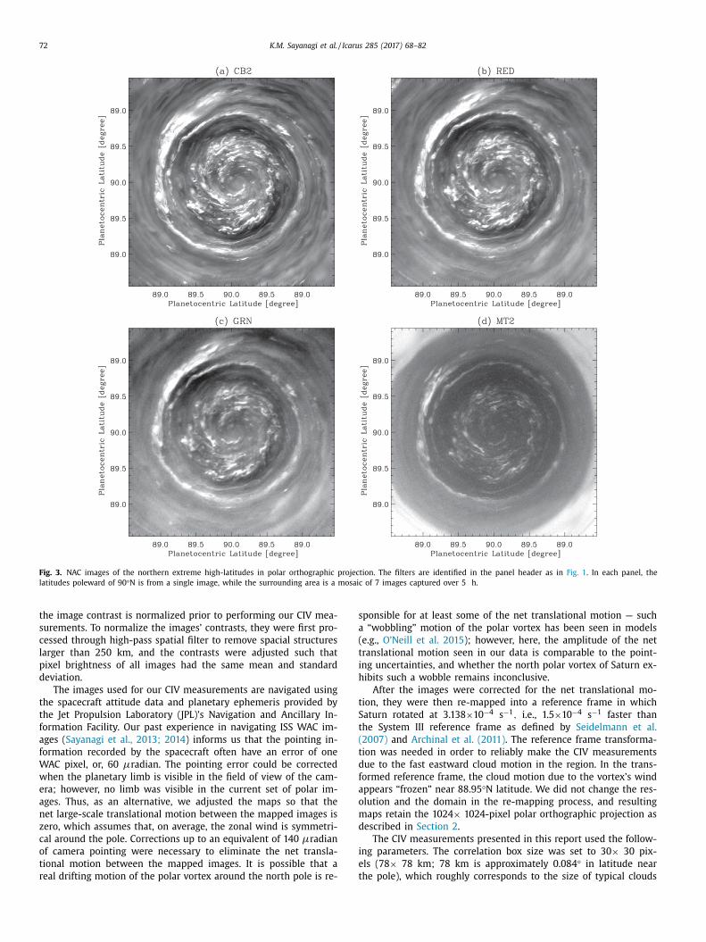
High-resolution morphology of the center of the polar vortex
s presented in Figs. 3 , 4 and 5 . Fig. 3 presents the NAC view of
he north pole; the figure shows a region within 1.5 ° of latitude
round the pole. These images are processed such that the region
oleward of 89 ° is from a single image, and the rest is a mosaic of
ultiple images to expand the view. The morphology in CB2, RED
nd GRN are very similar as exhibited in Fig. 2 panels a–c. In MT2,
he circular hole in the upper tropospheric haze is apparent; this
eature can also be seen in the WAC image ( Fig. 1 c). Inside of the
ole, only the brightest of the features that are visible in Figs. 3 a–c
re apparent. The CB2 and MT2 images were captured in the full-
esolution mode, while the RED, and GRN images were in the 2 × summation mode.
Fig. 4 shows the same region as in Fig. 3 in BL2 ( Fig. 4 a,
40 nm medium-band), UV3 ( Fig. 4 b, 343 nm broad-band) and
T3 ( Fig. 4 c) filters. These images are processed such that, for each
f the filters, 7 images captured over 5 h are averaged to improve
he image contrast. In addition, for the UV3 images, high-pass spa-
ial filter was applied to individual images prior to the averaging to
emove contrast variation spanning more than 1300 km (approxi-
ately 1.4 ° in latitude) and compensate for the imperfections in
he photometric flattening. Because the clouds in the polar vortex
egion move fast, in Fig. 4 , the averaging operation smeared indi-
idual small clouds that are apparent in Fig. 3 . We justify the aver-
ging because those small features are difficult to distinguish from
oise in the individual source images, and averaging multiple im-
ges helps in illustrating features symmetric around the pole. The
L2 view in Fig. 4 a exhibits the same hole in the cloud previously
resented in WAC views (BL1 and VIO, Figs. 1 g and 1 h). Unlike
he hole’s appearance in MT2, the hole’s morphology in BL2 has a
radual contrast change, and lacks a clear outline. In UV3 ( Fig. 4 b),
wo concentric circular structures surround the hole. Fig. 4 c shows
he view in MT3; the circular hole with a well-defined outline that
oughly follows the 88.5 °N latitude is the same feature as that seen
n MT2 ( Fig. 3 d); however, no cloud feature is visible inside of the
ark region. We did not find a high-latitude vortex that appears
nly in ultraviolet like that found on Jupiter by Porco et al. (2003) .
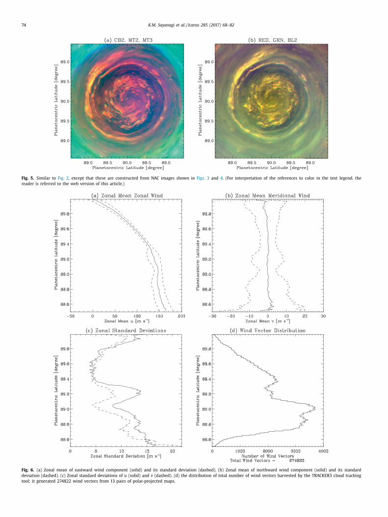
Fig. 5 shows the color overlay of the images that have been pre-
ented in Figs. 3 and 4 . In Fig. 5 a, the red, green and blue chan-
els are assigned to CB2, MT2 and MT3, respectively — this color
cheme is the same as in Fig. 2 a. A version without map-projection
as previously released in a NASA press release PIA14944. In
ig. 5 b, the red, green and blue channels are assigned to RED, GRN
nd BL2, respectively; this color scheme is the same as in Fig. 2 b.
.2. Cloud tracking wind measurement
In this section, we present results of cloud-tracking wind mea-
urement. To perform correlation imaging velocimetry (CIV) mea-
urements, we use TRACKER3, a CIV tool developed at JPL and
reviously applied to analyze wind fields on Jupiter ( Salyk et al.,
006 ) and Saturn ( Sayanagi et al., 2013; 2014 ). We tracked cloud
eatures in 14 of the NAC images captured over a period of 5 h
9 min on November 27, 2012. During the imaging sequence, CB2
nd RED images were captured alternately with a CB2-to-RED in-
erval of about 20 min and RED-to-CB2 interval of about 29 min;
e made CIV cloud-tracking measurements between these con-
ecutive CB2 and RED images. In a CIV measurement, it is usu-
lly not ideal to use images captured using different filters that
ay sense features at different altitudes; however, in the cur-
ent polar image sets, the appearance of cloud features is visu-
lly indistinguishable between CB2 and RED images (e.g., Fig. 3 a
nd b), and we found that the clouds in the region moved too
ast around the pole to take measurements with ∼ 50-min imag-
ng intervals between images using a single filter. For these rea-
ons, we found that it was more advantageous to track clouds
etween CB2 and RED images with 20 or 29 min intervals. The
mages were mapped in polar orthographic projection as described
n Section 2 . Orthographic projection shortens the apparent dis-
ance by approximately 0.02% at 88.5 °N, which does not pose an
ssue. Nevertheless, we circumvent the image distortion by mea-
uring the latitude-longitude coordinates of the tracked clouds, and
alculate their motion along Saturn’s oblate spherical surface. Be-
ause the CB2 and RED images have different ranges of I/F values,
72 K.M. Sayanagi et al. / Icarus 285 (2017) 68–82
Fig. 3. NAC images of the northern extreme high-latitudes in polar orthographic projection. The filters are identified in the panel header as in Fig. 1 . In each panel, the
latitudes poleward of 90 °N is from a single image, while the surrounding area is a mosaic of 7 images captured over 5 h.
s
a
(
t
i
h
t
S
t
(
t
d
f
a
o
m
d
i
e
t
the image contrast is normalized prior to performing our CIV mea-
surements. To normalize the images’ contrasts, they were first pro-
cessed through high-pass spatial filter to remove spacial structures
larger than 250 km, and the contrasts were adjusted such that
pixel brightness of all images had the same mean and standard
deviation.
The images used for our CIV measurements are navigated using
the spacecraft attitude data and planetary ephemeris provided by
the Jet Propulsion Laboratory (JPL)’s Navigation and Ancillary In-
formation Facility. Our past experience in navigating ISS WAC im-
ages ( Sayanagi et al., 2013; 2014 ) informs us that the pointing in-
formation recorded by the spacecraft often have an error of one
WAC pixel, or, 60 μradian. The pointing error could be corrected
when the planetary limb is visible in the field of view of the cam-
era; however, no limb was visible in the current set of polar im-
ages. Thus, as an alternative, we adjusted the maps so that the
net large-scale translational motion between the mapped images is
zero, which assumes that, on average, the zonal wind is symmetri-
cal around the pole. Corrections up to an equivalent of 140 μradian
of camera pointing were necessary to eliminate the net transla-
tional motion between the mapped images. It is possible that a
real drifting motion of the polar vortex around the north pole is re-
ponsible for at least some of the net translational motion — such
“wobbling” motion of the polar vortex has been seen in models
e.g., O’Neill et al. 2015 ); however, here, the amplitude of the net
ranslational motion seen in our data is comparable to the point-
ng uncertainties, and whether the north polar vortex of Saturn ex-
ibits such a wobble remains inconclusive.
After the images were corrected for the net translational mo-
ion, they were then re-mapped into a reference frame in which
aturn rotated at 3.138 ×10 −4 s −1 , i.e., 1.5 ×10 −4 s −1 faster than
he System III reference frame as defined by Seidelmann et al.
2007) and Archinal et al. (2011) . The reference frame transforma-
ion was needed in order to reliably make the CIV measurements
ue to the fast eastward cloud motion in the region. In the trans-
ormed reference frame, the cloud motion due to the vortex’s wind
ppears “frozen” near 88.95 °N latitude. We did not change the res-
lution and the domain in the re-mapping process, and resulting
aps retain the 1024 × 1024-pixel polar orthographic projection as
escribed in Section 2 .
The CIV measurements presented in this report used the follow-
ng parameters. The correlation box size was set to 30 × 30 pix-
ls (78 × 78 km; 78 km is approximately 0.084 ° in latitude near
he pole), which roughly corresponds to the size of typical clouds

K.M. Sayanagi et al. / Icarus 285 (2017) 68–82 73
Fig. 4. Same as in Fig. 3 , except that the maps here are average of 7 maps captured
over 5 h.
r
a
t
g
t
t
F
t
3
u
3
w
b
r
t
s
s
a
t
s
m
w
t
t
m
T
g
v
1
s
b
w
d
s
c
n
p
u
i
l
t
i
a
a
l
a
i
8
i
s
g
c
p
m
b
w
s
t
f
t
c
t
t
r
esolved in the NAC images. A tracking measurement was made on
cartesian grid with a grid separation of 5 pixels ( ∼ 13 km), i.e.,
here is a significant overlap in the correlation box between the
rids to ensure continuity in the returned wind field. The correla-
ion algorithm searched for a matching morphology in distance up
o 80 pixels away in the polar orthographic maps (about 210 km).
or an image pair with 20-min temporal separation, this correla-
ion search range combined with the reference frame change to
.138 ×10 −4 s −1 makes our measurements sensitive to wind speeds
p to 175 m s −1 at the pole and zonal wind speeds between
5 m s −1 and 315 m s −1 at 89 °N.
The zonal mean wind profiles returned by our cloud-tracking
ind measurements are shown in Fig. 6 . Fig. 6 d shows the distri-
ution of the wind vectors as a function of latitude; our analysis
eturned a total of 274,822 wind vectors; we binned the wind vec-
ors in latitude with a bin width of 0.01 °. The zonal mean and
tandard deviation of the eastward wind component u are pre-
ented in Fig. 6 a. Here, the zonal standard deviation of u and v
re the longitudinal variations in the measured value of u and v ;
hey do not represent measurement uncertainties. The zonal wind
peed steadily increases from the north pole to the end of the
easurement at 88.5 °N latitude. The zonal mean of the meridional
ind component v , shown in Fig. 6 b, is essentially zero throughout
he domain of measurement. The mapping process we used forces
he domain-mean meridional wind to become zero; however, our
easurements are sensitive to residual fluctuations around zero.
hus, our measurements did not detect zonally organized conver-
ence or divergence centered on the pole. The zonal standard de-
iations of both u and v stay between 3.7 m s −1 (at 89.52 °N) and
6 m s −1 (at 88.5 °N) throughout the latitudes covered in the mea-
urement.
The values of standard deviations include contributions from
oth real spatial variation in the wind and the uncertainty in the
ind measurements. Although our measurements do not provide a
irect way to distinguish the true spatial variations and the mea-
urement uncertainty, the zonal standard deviations of u and v
an be used to separate contributions from anisotropic compo-
ent of the spatial variation from the isotropic variation. Fig. 6 c
resents the zonal standard deviations of u and v ; when the val-
es of standard deviations are different, the wind vector variation
s spatially anisotropic. The maximum anisotropy occurs at 89.22 °Natitude, where the standard deviation of u is 5.7 m s −1 greater
han that of v ; if we assume that our measurement uncertainty is
sotropic, we can attribute this anisotropy in the wind vector vari-
tions to real spatial structures. The standard deviations of u and v
re essentially the same at 5–7 m s −1 between 89.4 °N and 89.8 °Natitudes, thus the wind vector variations are spatially isotropic
t these latitudes. However, the uncertainties of CIV cloud track-
ng methods are highly dependent on the cloud morphology. At
9.22 °N, Fig. 3 a shows that the clouds appear as streaks oriented
n east-west directions, which increases the uncertainty of u ; con-
equently, it is not surprising that the standard deviation of u is
reater than that of v . In the worst case, the measurement un-
ertainty is responsible for all of the standard deviation. We ex-
ect that, even in the absolute worst case, the correlation feature
atch can have a tracking uncertainty of quarter of the correlation
ox size, which is about 15 km in our current measurement. This
ould result in the wind speed uncertainty of 16 m s −1 ; Fig. 6 c
hows that the zonal standard deviations of u and v are substan-
ially smaller than 16 m s −1 in almost all latitudes. As a reference,
or an image pair with 20 min temporal separation, the uncer-
ainty of 10 m s −1 and 5 m s −1 would represent a tracking un-
ertainty of about 12 km and 6 km, respectively. Those uncertain-
ies correspond to about 15% and 7.5% of the size of the correla-
ion box, or 4.3 pixels and 2.2 pixels in the polar-projected maps,
espectively.
74 K.M. Sayanagi et al. / Icarus 285 (2017) 68–82
Fig. 5. Similar to Fig. 2 , except that these are constructed from NAC images shown in Figs. 3 and 4 . (For interpretation of the references to color in the text legend, the
reader is referred to the web version of this article.)
Fig. 6. (a) Zonal mean of eastward wind component (solid) and its standard deviation (dashed). (b) Zonal mean of northward wind component (solid) and its standard
deviation (dashed). (c) Zonal standard deviations of u (solid) and v (dashed). (d) the distribution of total number of wind vectors harvested by the TRACKER3 cloud tracking
tool; it generated 274822 wind vectors from 13 pairs of polar-projected maps.

K.M. Sayanagi et al. / Icarus 285 (2017) 68–82 75
Fig. 7. Map of eastward (panel a) and northward (b) wind components generated using a pair of polar-projected maps. Dark regions areas are where no trackable cloud was
found. Panels (c) and (d) show the same data as panels (a) and (b) except that the gaps filled using bi-linear interpolation method.
3
g
t
w
fi
a
c
F
p
r
d
t
fi
w
t
p
j
s
V
g
a
a
U
w
t
ζ
S
δ
W
�
t
r
.3. Relative vorticity and divergence
In this subsection, we present the relative vorticity and diver-
ence of the wind field in the north polar vortex. We calculate
he vorticity and divergence using the results of the cloud-tracking
ind measurements presented in the previous subsection. We first
ll the gaps in the wind field using bi-linear interpolation. Fig. 7 a
nd b present the zonal and meridional wind components of the
loud-tracking measurements — the cloud tracking result shown in
ig. 7 is from the cloud tracking performed between cloud maps
resented in Figs. 3 a and b. In the figures, the black pixels rep-
esent areas where no trackable pattern was detected. Fig. 7 c and
show the same wind fields with the gaps interpolated. The vor-
icity and divergence were calculated using the interpolated wind
eld.
After the gaps in the wind field are filled through interpolation,
e calculate the relative vorticity and divergence. Our wind vec-
ors are calculated on a cartesian grid ( i, j ) superimposed on the
olar orthographic map projection. The cartesian grid indices i and
increase in the directions of 0 ° and 90 ° eastward longitude, re-
pectively. We denote the cartesian wind components as U i, j and
i, j . U i, j and V i, j blow in the direction of 0 ° and 90 ° eastward lon-
itude, respectively. The cartesian wind components U i, j and V i, j
re related to the eastward and northward wind components u i, j nd v i, j by
i, j = −u i, j sin (λi, j ) − v i, j cos (λi, j )
V i, j = u i, j cos (λi, j ) − v i, j sin (λi, j ) , (1)
here λi, j is the eastward longitude. On grid ( i, j ), the relative vor-
icity then becomes
i, j =
V i +1 , j − V i −1 , j
�X i, j
− U i, j+1 − U i, j−1
�Y i, j
. (2)
imilarly, the divergence is
i, j =
U i, j+1 − U i, j−1
�X i, j
+
V i, j+1 − V i, j−1
�Y i, j
. (3)
e take account of Saturn’s oblateness in calculating the distances
X i, j and �Y i, j using the following oblate spherical mapping fac-
ors
i, j =
R e
1 + (R p /R e ) 2 tan
2 ϕ i, j
(4)
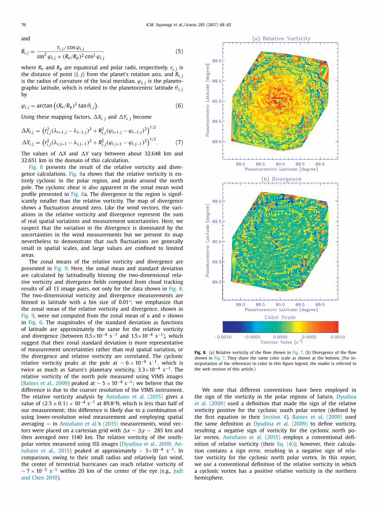
76 K.M. Sayanagi et al. / Icarus 285 (2017) 68–82
Fig. 8. (a) Relative vorticity of the flow shown in Fig. 7 . (b) Divergence of the flow
shown in Fig. 7 . They share the same color scale as shown at the bottom. (For in-
terpretation of the references to color in this figure legend, the reader is referred to
the web version of this article.)
t
e
v
t
t
r
l
n
t
t
w
a
h
and
R i, j =
r i, j / cos ϕ i, j
sin
2 ϕ i, j + (R e /R p ) 2 cos 2 ϕ i, j
(5)
where R e and R p are equatorial and polar radii, respectively. r i, j is
the distance of point ( i, j ) from the planet’s rotation axis, and R i, j is the radius of curvature of the local meridian. ϕi, j is the planeto-
graphic latitude, which is related to the planetocentric latitude θ i, j
by
ϕ i, j = arctan
((R e /R p )
2 tan θi, j
). (6)
Using these mapping factors, �X i, j and �Y i, j become
�X i, j =
(r 2 i, j (λi +1 , j − λi −1 , j )
2 + R
2 i, j (ϕ i +1 , j − ϕ i −1 , j )
2 )1 / 2
�Y i, j =
(r 2 i, j (λi, j+1 − λi, j−1 )
2 + R
2 i, j (ϕ i, j+1 − ϕ i, j−1 )
2 )1 / 2
. (7)
The values of �X and �Y vary between about 32.648 km and
32.651 km in the domain of this calculation.
Fig. 8 presents the result of the relative vorticity and diver-
gence calculations. Fig. 8 a shows that the relative vorticity is en-
tirely cyclonic in the polar region, and peaks around the north
pole. The cyclonic shear is also apparent in the zonal mean wind
profile presented in Fig. 6 a. The divergence in the region is signif-
icantly smaller than the relative vorticity. The map of divergence
shows a fluctuation around zero. Like the wind vectors, the vari-
ations in the relative vorticity and divergence represent the sum
of real spatial variations and measurement uncertainties. Here, we
suspect that the variation in the divergence is dominated by the
uncertainties in the wind measurements but we present its map
nevertheless to demonstrate that such fluctuations are generally
small in spatial scales, and large values are confined to limited
areas.
The zonal means of the relative vorticity and divergence are
presented in Fig. 9 . Here, the zonal mean and standard deviation
are calculated by latitudinally binning the two-dimensional rela-
tive vorticity and divergence fields computed from cloud tracking
results of all 13 image pairs, not only for the data shown in Fig. 8 .
The two-dimensional vorticity and divergence measurements are
binned in latitude with a bin size of 0.01 °; we emphasize that
the zonal mean of the relative vorticity and divergence, shown in
Fig. 9 , were not computed from the zonal mean of u and v shown
in Fig. 6 . The magnitudes of the standard deviation as functions
of latitude are approximately the same for the relative vorticity
and divergence (between 0.5 ×10 −4 s −1 and 1.5 ×10 −4 s −1 ), which
suggest that their zonal standard deviation is more representative
of measurement uncertainties rather than real spatial variation, or
the divergence and relative vorticity are correlated. The cyclonic
relative vorticity peaks at the pole at ∼ 6 × 10 −4 s −1 , which is
twice as much as Saturn’s planetary vorticity, 3.3 ×10 −4 s −1 . The
relative vorticity of the north pole measured using VIMS images
( Baines et al., 2009 ) peaked at ∼ 5 × 10 −4 s −1 ; we believe that the
difference is due to the coarser resolution of the VIMS instrument.
The relative vorticity analysis by Antuñano et al. (2015) gives a
value of (2 . 5 ± 0 . 1) × 10 −4 s −1 at 89.8 °N, which is less than half of
our measurement; this difference is likely due to a combination of
using lower-resolution wind measurement and employing spatial
averaging — in Antuñano et al. ’s (2015) measurements, wind vec-
tors were placed on a cartesian grid with �x ∼ �y ∼ 285 km and
then averaged over 1140 km. The relative vorticity of the south-
polar vortex measured using ISS images ( Dyudina et al., 2009; An-
tuñano et al., 2015 ) peaked at approximately – 3 ×10 −4 s −1 . In
comparison, owing to their small radius and relatively fast wind,
the center of terrestrial hurricanes can reach relative vorticity of
∼ 7 × 10 −3 s −1 within 20 km of the center of the eye (e.g., Judt
and Chen 2010 ).
We note that different conventions have been employed in
he sign of the vorticity in the polar regions of Saturn. Dyudina
t al. (2009) used a definition that made the sign of the relative
orticity positive for the cyclonic south polar vortex (defined by
he first equation in their Section 4 ). Baines et al. (2009) used
he same definition as Dyudina et al. (2009) to define vorticity,
esulting a negative sign of vorticity for the cyclonic north po-
ar vortex. Antuñano et al. (2015) employs a conventional defi-
ition of relative vorticity (their Eq. (4) ); however, their calcula-
ion contains a sign error, resulting in a negative sign of rela-
ive vorticity for the cyclonic north polar vortex. In this report,
e use a conventional definition of the relative vorticity in which
cyclonic vortex has a positive relative vorticity in the northern
emisphere.

K.M. Sayanagi et al. / Icarus 285 (2017) 68–82 77
Fig. 9. (a) Zonal mean of the relative vorticity of wind measurements in all 13 map
pairs. (b) Same as panel (a), except that it shows the divergence.
4
p
a
v
2
t
w
p
c
o
t
C
e
9
t
l
t
i
G
∼
s
t
w
o
t
t
i
v
T
b
w
t
t
(
p
s
t
t
(
(
c
h
a
F
l
u
m
a
b
o
n
h
m
s
a
r
t
b
o
a
o
t
c
m
M
a
c
a
B
c
i
T
r
h
t
d
D
a
. Comparison to Saturn’s south pole
In this section, we compare the cloud morphology of the north-
olar vortex to that of the south-polar vortex. The morphology
nd dynamics of Saturn’s south pole has been documented pre-
iously by Sánchez-Lavega et al. (2006) , Dyudina et al. (2008,
009) and Antuñano et al. (2015) . These previous papers presented
he morphology of the south pole using CB2 and CB3 images,
hich showed, like the north pole, the clouds around the south
ole exhibit cyclonically spiraling (i.e., a spiral arm turns counter-
lockwise as it extends away from the pole) morphology centered
n the pole and extending down to around 83 °S.
Here, we extend the morphological analysis to the images cap-
ured using MT2, MT3, RED, GRN, BL1 and VIO filters in addition to
B2 and CB3. On January 30–31, 2007, 9 images were captured in
ach of the filters over a duration of 3 h 20 min; we averaged the
map-projected images captured in each of the filters to improve
he contrast, and show the results for each of the filters in Fig. 10 .
Fig. 10 presents polar-projected maps of the southern high-
atitude region. The double-wall structure surrounding the “eye” of
he south polar vortex, originally reported by Dyudina et al. (2008) ,
s apparent when viewed in CB2 ( Fig. 10 a), CB3 (10b), RED (10e),
RN (10f) and BL1 (10g). The two walls are located at ∼ 88 °S and
89 °S. In those filters, the interior of the eye appears dark. Out-
ide of the eye, concentric albedo structure that appears substan-
ially brighter than the eye interior dominates the morphology, in
hich a few diffuse discrete features can also be seen. The interior
f the eye also appears dark in MT2 Fig. 10 c) and MT3 (10d). While
he interior of the eye of the south-polar vortex appears darker
han the surrounding in all above filters, the contrast is reversed
n VIO ( Fig. 10 h), in which a bright cloud covers the south-polar
ortex eye region poleward of 87 °S, which we call the polar cap.
he bright polar cap is apparent only in the VIO filter presumably
ecause the aerosol layer that forms the cap is in the stratosphere,
here it scatters light more in the shorter wavelengths sensed by
he VIO filter.
The presence of the bright cap visible in VIO is consistent with
he warm summer south polar region observed by Cassini CIRS
Fletcher et al., 2008; 2015 ). Fletcher et al. (2008, 2015) inter-
reted the warming of the south pole to be a result of solar ab-
orption by stratospheric aerosols formed through photodissocia-
ion of methane molecules and trapped in the south polar vor-
ex. Our observation of the bright polar cap over the south pole
Fig. 10 h) was taken in 2007 shortly before the equinox in 2009
late summer), while the north polar images without a cap were
aptured in 2012 (early spring). The photochemical production of
aze particles in giant planet stratospheres is described by Atreya
nd Wong (2005) , Wong et al. (2003) and West et al. (2009) . Like
letcher et al. (2008, 2015) , we interpret the presence of a haze
ayer over the summer pole as an indication that it is a result of
ltraviolet photodissociation of hydrocarbon molecules in the sum-
er polar stratosphere. If Saturnian bright polar caps consist of
erosols formed through ultraviolet photodissociation of hydrocar-
ons, this interpretation also explains the absence of a similar cap
ver the north pole in 2012 because the north polar region had
ot received sufficient insolation to have formed a photochemical
aze layer. This hypothesis may be tested by the Cassini extended
ission by observing whether a cap similar to that seen over the
outh pole in 2007 will form over the north pole as the north pole
pproaches the next solstice in 2017.
As shown in Fig. 10 c, in MT2, the brightness of the eye inte-
ior appears to decrease in three discrete steps; the clouds appear
he brightest outside of the outer wall at 87 °S latitude. The region
etween 87 °S and 88 °S (which roughly coincides the outer edge
f the inner wall structure) constitutes the first step down in the
lbedo value. The region between 88 °S and 89 °S forms the sec-
nd step. Poleward of 89 °S is the third step, where the albedo is
he darkest in the south-polar region seen in MT2; 89 °S roughly
orresponding to the inner edge of the inner wall structure. The
orphology in MT3 appears ( Fig. 10 d) generally similar to that in
T2, except that the boundaries between the albedo steps are not
s sharp.
Fig. 11 a presents a false-color view in which red, green and blue
hannels are assigned to CB2, MT2, and MT3 maps like in Fig. 2 a
nd Fig. 5 a. Fig. 11 b assigns the RGB channels to RED, GRN and
L1 maps like in Figs. 2 b and 5 b, showing a contrast-enhanced real
olor view of the south pole.
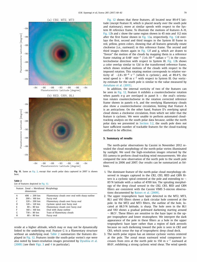
We also analyze the morphologies and the motions of clouds
nside the south polar vortex’s inner eye-wall, shown in Fig. 12 .
hree NAC images captured using the CB2 filter on July 14, 2008
evealed multiple discrete clouds that can be tracked over two
ours. The first of the three images is shown in Fig. 12 a (with fea-
ure labels) and 12e (without labels). Features A and F have well-
efined oval shapes with sharply resolved outlines. Features B, C,
, E and H also have oval shapes, but have gradually fading bound-
ries. Features A, C, D and E have filamentary clouds that appear to

78 K.M. Sayanagi et al. / Icarus 285 (2017) 68–82
Fig. 10. Same as Fig. 1 , except that south polar data captured in 2007 is shown here.
K.M. Sayanagi et al. / Icarus 285 (2017) 68–82 79
Fig. 11. Same as Fig. 2 , except that south polar data captured in 2007 is shown
here.
Table 2
List of features depicted in Fig. 12 .
Feature Zonal × Meridional
dimensions
Morphology
A 490 × 200 km Filamentary clouds over oval with sharp outline
B 200 × 160 km Fuzzy oval
C 320 × 200 km Filamentary clouds over fuzzy oval
D 120 × 120 km Cyclonic spiral over fuzzy oval
E 80 × 80 km Filamentary clouds over fuzzy oval
F 160 × 160 km Oval with sharp outline
G 730 × 80 km Train of filamentary clouds
H 80 × 80 km Fuzzy oval
r
l
w
p
a
(
t
a
t
F
a
l
r
c
t
“
f
t
a
w
i
t
w
i
A
b
w
t
f
a
i
c
f
t
p
h
m
5
v
b
I
c
o
l
eside at a higher altitude, which may or may not be dynamically
inked to the underlying oval. Feature G is a filamentary structure
ithout an underlying oval. Table 2 summarizes the features dis-
layed in Fig. 12 . Features inside the south-polar vortex’s eye were
lso noted by lower-resolution images presented by Dyudina et al.
2009) (see their Figs. 3 and 4 in particular).
Fig. 12 shows that these features, all located near 89.4 °S lati-
ude (except Feature H, which is placed nearly over the south pole
nd stationary), move at similar speeds with respect to the Sys-
em III reference frame. To illustrate the motions of features A–H,
ig. 12 b and c show the same region shown in 45 min and 112 min
fter the first frame shown in Fig. 12 a, respectively. Fig. 12 d over-
ays the first, second and third images in the System III frame in
ed, yellow, green colors, showing that all features generally rotate
lockwise (i.e., eastward) in this reference frame. The second and
hird images shown again in Fig. 12 f and g, which are drawn to
freeze” the motion of the clouds by mapping them in a reference
rame rotating at 0.48 ° min
−1 (1.4 ×10 −4 radian s −1 ) in the coun-
erclockwise direction with respect to System III. Fig. 12 h shows
color overlay similar to 12d in the transformed reference frame,
hich shows residual motions of the clouds with respect to the
mposed rotation. This rotating motion corresponds to relative vor-
icity of –2.8 ×10 −4 s −1 (which is cyclonic), and, at 89.4 °S, the
ind speed is ∼ 80 m s −1 with respect to System III. Our vortic-
ty estimate for the south pole is similar to the value measured by
ntuñano et al. (2015) .
In addition, the internal vorticity of two of the features can
e seen in Fig. 12 . Feature A exhibits a counterclockwise rotation
hen panels e-g are overlayed in panel h — the oval’s orienta-
ion rotates counterclockwise in the rotation corrected reference
rame shown in panels e-h, and the overlying filamentary clouds
lso show a counterclockwise circulation, hinting that Feature A
s an anticyclone. On the other hand, Feature D’s overlying spiral
loud shows a clockwise circulation, from which we infer that the
eature is cyclonic. We were unable to perform automated cloud-
racking analysis on the south polar data because, unlike the north
olar data we presented in Section 3.2 , the south pole does not
ave sufficient number of trackable features for the cloud-tracking
ethod to be effective.
. Summary of results
The north-polar observations by Cassini in November 2012 re-
ealed the cloud morphology of the north-polar vortex illuminated
y sunlight. We used the high-resolution images returned by the
SS camera to perform cloud-tracking wind measurements. We also
ompared the new observation of the north pole to the south pole
bserved in 2006 and 2007. Our results can be summarized as fol-
ows.
1. The dominant feature of the north-polar cloud morphology ob-
served in images captured in the CB2, CB3, RED and GRN fil-
ters is a cyclonic spiral centered at the pole and extending to ∼85 °N latitude with a radius of 4700 km. The spiraling morphol-
ogy of the deep cloud sensed in the CB2, CB3, RED and GRN
filters are consistent with the Cassini VIMS 5-micron observa-
tions documented by Baines et al. (2009) .
2. The upper tropospheric haze layer detected in the MT2, MT3,
BL1 and VIO filters shows a dark circular hole centered at the
pole. In the MT2 and MT3 filters, the outline of the hole, lo-
cated at 88.5 °N latitude, is sharp. The hole seen in the BL1
and VIO shows a gradual poleward darkening starting around
∼ 88.5 °. These filters are sensitive to the haze layer in the up-
per troposphere and lower stratosphere. We interpret the dark
appearance of the pole in these filters as a hole in the upper
tropospheric haze layer rather than a region of dark aerosols
because no such darkening toward the pole is seen in CB2 and
CB3, which sense the top of tropospheric deep cloud deck.
3. The north polar region has an intense cyclonic vortex centered
at the pole. The zonal mean eastward wind component in-
creases from zero at the north pole to 150 m s −1 eastward at
89.0 °, exhibiting a strong cyclonic wind shear. The wind speeds

80
K.M
. Sa
yan
ag
i et
al. / Ica
rus 2
85 (2
017
) 6
8–
82
Fig. 12. NAC images of the southern extreme high-latitudes poleward of – 89.28 °S in polar orthographic projection, captured in 2008 using the CB2 filter. Panel (a)–(c) show the region in three successive images separated by
approximately 45 min between (a) and (b), and 67 min between (b) and (c). Panel (d) overlays the images presented in panels (a)–(c) in red, yellow and green color channels to illustrate the cloud motion in the System III
reference frame. Panels (e)–(h) show the same, except that they are rotated counterclockwise (i.e., westward) with respect to panel (a) at 0.48 ° per min (1.4 ×10 −4 radian s −1 ) to ‘freeze’ the cloud motion. The features labeled A–H
are discussed in the main text. (For interpretation of the references to color in this figure legend, the reader is referred to the web version of this article.)

K.M. Sayanagi et al. / Icarus 285 (2017) 68–82 81
o
B
t
b
c
2
t
g
t
f
t
p
f
p
r
m
t
c
b
f
a
t
r
O
t
e
t
l
g
w
t
i
m
t
r
m
p
n
2
t
c
l
i
m
p
m
c
A
c
s
w
R
g
G
1
a
R
A
A
A
A
B
B
C
D
D
D
D
EF
F
detected here are consistent with that measured by Baines et al.
(2009) for the north pole. The wind structure at the north pole
is similar to that at the south pole revealed by Baines et al.
(2009) and Dyudina et al. (2009) .
4. The relative vorticity peaks at ∼ 6 × 10 −4 s −1 at the north pole,
which is a factor of two greater than the planetary vorticity.
The value measured here is greater than the values previously
measured by Antuñano et al. (2015) ( (2 . 5 ± 0 . 1) × 10 −4 s −1 ) us-
ing lower-resolution ISS images, and Baines et al. (2009) ( (5 ±0 . 5) × 10 −4 s −1 ) using VIMS 5-micron images; we believe that
these earlier measurements did not resolve the peak at the
pole due to the lower resolutions of the images employed in
their studies. In numerical simulations by O’Neill et al. (2015,
2016) for a Saturn-like case, the vortices gain relative vorticity
of up to 1.5 times the planetary vorticity. The dynamical impli-
cation of the high polar relative vorticity value is unclear.
5. The magnitude of the zonal mean divergence of the wind field
is smaller than 10 −5 s −1 , beyond the detection limit of the cur-
rent study.
6. The south polar vortex exhibits two concentric eye walls at ∼88 °S and ∼ 89 °S in CB2, CB3, RED, GRN and BL1 wavelengths.
7. In 2007, the south polar region at latitudes higher than ∼ 87 °Swas covered in a bright polar cap visible in the VIO filter. We
interpret the presence of the cap in the summer pole as a
result of stratospheric photochemical haze production through
mechanisms described by Atreya and Wong (2005) , Wong et al.
(2003) and West et al. (2009) . If the haze particles indeed form
over a summer pole, we expect a similar polar cap to form over
the north pole as it approaches the next solstice in 2017.
8. Discrete clouds can be seen in the interior of the inner eye wall
of the south polar vortex. From the motion of the clouds, the
relative vorticity is estimated to be – 2.8 ×10 −4 s −1 (which is
cyclonic). The relative vorticity structure of the south pole mea-
sured by Dyudina et al. (2009) and Antuñano et al. (2015) was
3 × 10 −4 s −1 .
The Cassini discoveries of intense polar cyclones at both poles
f Saturn are intriguing. Scott (2011) , O’Neill et al. (2015, 2016) and
rueshaber and Sayanagi (2014) used numerical models to show
hat turbulence leads to poleward flux of cyclonic vorticity through
eta-drifting cyclones, and results in an accumulation of cy-
lonic vorticity at the pole. In particular, O’Neill et al. (2015,
016) demonstrated that the ratio of the planetary radius a and
he Rossby deformation radius L D is a key parameter that controls
iant planet polar atmospheric dynamics. They showed that an in-
ense polar vortex forms when the model used a strong turbulent
orcing and a Saturn-like size ratio of a/L D ∼ 20 ; under this regime,
he relative vorticity of the polar vortex became greater than the
lanetary vorticity by a factor of ∼ 1.5. Under weak mechanical
orcing and a/L D ∼ 20 , O’Neill et al. (2015) produced a transient
olar cyclone, which the authors hypothesized as a Neptune-like
egime. For a Jupiter-like planetary size ratio of a/L D ∼ 40 , the
odel produced turbulent flows with weak zonal organization like
hat of Jupiter’s high latitudes regardless of the forcing strength.
Comparison of the Saturnian polar vortices with terrestrial cy-
lones illustrates some interesting commonalities and differences
etween them. First, terrestrial hurricanes require a warm sea sur-
ace to form ( Anthes, 1982; Houze, 1993; Emanuel, 2003 ); such
n energy source is not available on the giant planets. Although
he formation process differs, the intensification of terrestrial hur-
icanes follows a process similar to that tested by Scott (2011) and
’Neill et al. (2015, 2016) . In addition to the latent heat flux from
he surface, when a terrestrial tropical cyclone becomes intense
nough, it creates a local peak in the potential vorticity field such
hat it generates a local effective β-effect. The process involving
ocal effective- β is analogous to the planetary- β , which is the
radient of the planetary vorticity, and the results are similar;
hen cumulus convection generates eddies inside of a terrestrial
ropical cyclone, it causes an inward flux of cyclonic vorticity, and
ntensifies the cyclone ( Montgomery and Enagonio, 1998 ). Further
odeling effort s under more realistic conditions (e.g., inclusion of
he vertical dimension so that baroclinic effects are realistically
epresented) and observational studies to measure the eddy mo-
entum flux in the polar region (such measurements have been
erformed for mid-latitudes by Del Genio et al. (2007) and Del Ge-
io and Barbara (2012) ) may shed further light on this process.
If the differences in the morphology between the south pole in
007 and the north pole in 2012 were caused by seasonal effects,
he north pole, now basking in continuous sunshine, should be-
ome similar that of the south pole in 2007. In particular, if the po-
ar cap over the south pole in 2007, seen in the VIO filter ( Fig. 10 h),
s produced through ultraviolet photodissociation of hydrocarbon
olecules, we expect a similar bright cap to form over the north
ole later in the season. The continuing observation by the Cassini
ission should reveal whether seasonal effects will alter the polar
loud morphology.
cknowledgments
Our work was supported by the Cassini-Huygens mission, a
ooperative project of NASA, ESA, ASI, managed by JPL, a divi-
ion of the California Institute of Technology, under a contract
ith NASA. KMS acknowledges support from NASA Outer Planets
esearch Grant NNX12AR38G , NASA Planetary Atmospheres Pro-
ram Grant NNX14AK07G , NASA Cassini Data Analysis Program
rant NNX15AD33G , and NSF Astronomy and Astrophysics Grant
212216 . API acknowledges support from NSF grant AST-1411952
nd by the Cassini Project of NASA.
eferences
nthes, R.A. , 1982. Tropical Cyclones. Their Evolution, Structure and Effects. Ameri-
can Meteorological Society. . ntuñano, A. , Río-Gaztelurrutia, T. , Sánchez-Lavega, A. , Hueso, R. , 2015. Dynamics of
Saturn’s polar regions. J. Geophys. Res. 120, 155–176 . rchinal, B.A. , A’Hearn, M.F. , Bowell, E. , Conrad, A. , Consolmagno, G.J. , Courtin, R. ,
Fukushima, T. , Hestroffer, D. , Hilton, J.L. , Krasinsky, G.A. , Neumann, G. , Oberst, J. ,
Seidelmann, P.K. , Stooke, P. , Tholen, D.J. , Thomas, P.C. , Williams, I.P. , 2011. Re-port of the IAU Working Group on Cartographic Coordinates and Rotational El-
ements: 2009. Celestial Mech. Dyn. Astron. 109, 101–135 . treya, S.K. , Wong, A.-S. , 2005. Coupled clouds and chemistry of the giant planets
— a case for Multiprobes. Space Sci. Rev. 116, 121–136 . aines, K.H. , Momary, T.W. , Fletcher, L.N. , Showman, A.P. , Roos-Serote, M. ,
Brown, R.H. , Buratti, B.J. , Clark, R.N. , Nicholson, P.D. , 2009. Saturn’s north po-
lar cyclone and hexagon at depth revealed by Cassini/VIMS. Planet. Space Sci.57, 1671–1681 .
rueshaber, S.R. , Sayanagi, K.M. , 2014. Numerical simulations of Saturn’s polar cy-clones. In: AAS/Division for Planetary Sciences Meeting Abstracts. Vol. 46 of
AAS/Division for Planetary Sciences Meeting Abstracts, p. 422.27 . aldwell, J. , Hua, X.-M. , Turgeon, B. , Westphal, J.A. , Barnet, C.D. , 1993. The drift of
Saturn’s north polar SPOT observed by the Hubble Space Telescope. Science 260,
326–329 . el Genio, A.D. , Barbara, J.M. , 2012. Constraints on Saturn’s tropospheric general
circulation from Cassini ISS images. Icarus 219, 689–700 . el Genio, A.D. , Barbara, J.M. , Ferrier, J. , Ingersoll, A.P. , West, R.A. , Vasavada, A.R. ,
Spitale, J. , Porco, C.C. , 2007. Saturn eddy momentum fluxes and convection: firstestimates from Cassini images. Icarus 189, 479–492 .
yudina, U.A . , Ingersoll, A .P. , Ewald, S.P. , Vasavada, A .R. , West, R.A . , Baines, K.H. ,
Momary, T.W. , Del Genio, A.D. , Barbara, J.M. , Porco, C.C. , Achterberg, R.K. ,Flasar, F.M. , Simon-Miller, A .A . , Fletcher, L.N. , 2009. Saturn’s south polar vortex
compared to other large vortices in the Solar system. Icarus 202, 240–248 . yudina, U.A. , Ingersoll, A.P. , Ewald, S.P. , Vasavada, A.R. , West, R.A. , Del Genio, A.D. ,
Barbara, J.M. , Porco, C.C. , Achterberg, R.K. , Flasar, F.M. , Simon-Miller, A .A . ,Fletcher, L.N. , 2008. Dynamics of Saturn’s south polar vortex. Science 319, 1801 .
manuel, K. , 2003. Tropical cyclones. Ann. Rev Earth Planet. Sci. 31, 75–104 . letcher, L.N. , Irwin, P.G.J. , Orton, G.S. , Teanby, N.A. , Achterberg, R.K. , Bjoraker, G.L. ,
Read, P.L. , Simon-Miller, A .A . , Howett, C. , de Kok, R. , Bowles, N. , Calcutt, S.B. ,
Hesman, B. , Flasar, F.M. , 2008. Temperature and composition of Saturn’s polarhot spots and hexagon. Science 319, 79–81 .
letcher, L.N. , Irwin, P.G.J. , Sinclair, J.A. , Orton, G.S. , Giles, R.S. , Hurley, J. , Gorius, N. ,Achterberg, R.K. , Hesman, B.E. , Bjoraker, G.L. , 2015. Seasonal evolution of Sat-
urn’s polar temperatures and composition. Icarus 250, 131–153 .

82 K.M. Sayanagi et al. / Icarus 285 (2017) 68–82
S
S
S
S
S
S
T
V
W
W
W
García-Melendo, E. , Pérez-Hoyos, S. , Sánchez-Lavega, A. , Hueso, R. , 2011. Saturn’szonal wind profile in 20 04–20 09 from Cassini ISS images and its long-term
variability. Icarus 215, 62–74 . García-Melendo, E. , Sánchez-Lavega, A. , Rojas, J.F. , Pérez-Hoyos, S. , Hueso, R. , 2009.
Vertical shears in Saturn’s eastward jets at cloud level. Icarus 201, 818–820 . Godfrey, D.A. , 1988. A hexagonal feature around Saturn’s north pole. Icarus 76,
335–356 . Houze, R.A. , 1993. Cloud Dynamics. Academic Press, San Diego, CA .
Judt, F. , Chen, S.S. , 2010. Convectively generated potential vorticity in rainbands and
formation of the secondary eyewall in hurricane Rita of 2005. J. Atmosph. Sci.67, 3581–3599 .
Lindal, G.F. , Sweetnam, D.N. , Eshleman, V.R. , 1985. The atmosphere of Saturn –an analysis of the Voyager radio occultation measurements. Astron. J. 90,
1136–1146 . Montgomery, M.T. , Enagonio, J. , 1998. Tropical cyclogenesis via convectively forced
vortex Rossby waves in a three-dimensional quasigeostrophic model. J. Atmo-
sph. Sci. 55, 3176–3207 . O’Neill, M.E. , Emanuel, K.A. , Flierl, G.R. , 2015. Polar vortex formation in giant-planet
atmospheres due to moist convection. Nat. Geosci. 8, 523–526 . O’Neill, M.E. , Emanuel, K.A. , Flierl, G.R. , 2016. Weak jets and strong cyclones: shal-
low-water modeling of giant planet polar caps. J. Atmosph. Sci. 73, 1841–1855 . Porco, C.C. , Baker, E. , Barbara, J. , Beurle, K. , Brahic, A. , Burns, J.A. , Charnoz, S. ,
Cooper, N. , Dawson, D.D. , Del Genio, A.D. , Denk, T. , Dones, L. , Dyudina, U. ,
Evans, M.W. , Giese, B. , Grazier, K. , Helfenstein, P. , Ingersoll, A.P. , Jacobson, R.A. ,Johnson, T.V. , McEwen, A. , Murray, C.D. , Neukum, G. , Owen, W.M. , Perry, J. ,
Roatsch, T. , Spitale, J. , Squyres, S. , Thomas, P. , Tiscareno, M. , Turtle, E. ,Vasavada, A.R. , Veverka, J. , Wagner, R. , West, R. , 2005. Cassini imaging science:
initial results on Saturn’s atmosphere. Science 307, 1243–1247 . Porco, C.C. , West, R.A. , McEwen, A. , Del Genio, A.D. , Ingersoll, A.P. , Thomas, P. ,
Squyres, S. , Dones, L. , Murray, C.D. , Johnson, T.V. , Burns, J.A. , Brahic, A. ,
Neukum, G. , Veverka, J. , Barbara, J.M. , Denk, T. , Evans, M. , Ferrier, J.J. , Geissler, P. ,Helfenstein, P. , Roatsch, T. , Throop, H. , Tiscareno, M. , Vasavada, A.R. , 2003.
Cassini imaging of Jupiter’s atmosphere, satellites, and rings. Science 299,1541–1547 .
Porco, C.C. , West, R.A. , Squyres, S. , McEwen, A. , Thomas, P. , Murray, C.D. , Del Ge-nio, A. , Ingersoll, A.P. , Johnson, T.V. , Neukum, G. , Veverka, J. , Dones, L. , Brahic, A. ,
Burns, J.A. , Haemmerle, V. , Knowles, B. , Dawson, D. , Roatsch, T. , Beurle, K. ,
Owen, W. , 2004. Cassini imaging science: instrument characteristics and antici-pated scientific investigations at Saturn. Space Sci. Rev. 115, 363–497 .
alyk, C. , Ingersoll, A.P. , Lorre, J. , Vasavada, A. , Del Genio, A.D. , 2006. Interaction be-tween eddies and mean flow in Jupiter’s atmosphere: analysis of Cassini imag-
ing data. Icarus 185, 430–442 . ánchez-Lavega, A. , Hueso, R. , Pérez-Hoyos, S. , Rojas, J.F. , 2006. A strong vortex in
Saturn’s south pole. Icarus 184, 524–531 . anchez-Lavega, A. , Lecacheux, J. , Colas, F. , Laques, P. , 1993. Ground-based observa-
tions of Saturn’s north polar SPOT and hexagon. Science 260, 329–332 . Sanchez-Lavega, A. , Rojas, J.F. , Acarreta, J.R. , Lecacheux, J. , Colas, F. , Sada, P.V. , 1997.
New observations and studies of Satusrn’s long-lived north polar SPOT. Icarus
128, 322–334 . ayanagi, K.M. , Dyudina, U.A. , Ewald, S.P. , Fischer, G. , Ingersoll, A.P. , Kurth, W.S. ,
Muro, G.D. , Porco, C.C. , West, R.A. , 2013. Dynamics of Saturn’s great storm of2010-2011 from Cassini ISS and RPWS. Icarus 223, 460–478 .
ayanagi, K.M. , Dyudina, U.A. , Ewald, S.P. , Muro, G.D. , Ingersoll, A.P. , 2014. CassiniISS observation of Saturn’s string of pearls. Icarus 229, 170–180 .
Scott, R.K. , 2011. Polar accumulation of cyclonic vorticity. Geophys. Astrophys. Fluid
Dyn. 105, 409–420 . eidelmann, P.K. , Archinal, B.A. , A’Hearn, M.F. , Conrad, A. , Consolmagno, G.J. , He-
stroffer, D. , Hilton, J.L. , Krasinsky, G.A. , Neumann, G. , Oberst, J. , Stooke, P. ,Tedesco, E.F. , Tholen, D.J. , Thomas, P.C. , Williams, I.P. , 2007. Report of the
IAU/IAG working group on cartographic coordinates and rotational elements:2006. Celestial Mech. Dyn. Astron. 98, 155–180 .
omasko, M.G. , West, R.A. , Orton, G.S. , Teifel, V.G. , 1984. In: Gehrels, T.,
Matthews, M.S. (Eds.), Clouds and aerosols in Saturn’s atmosphere. Saturn. Univ.of Arizona Press, Tucson, pp. 150–194 .
asavada, A.R. , Hörst, S.M. , Kennedy, M.R. , Ingersoll, A.P. , Porco, C.C. , Del Genio, A.D. ,West, R.A. , 2006. Cassini imaging of Saturn: southern hemisphere winds and
vortices. J. Geophys. Res. (Planets) 111, E05004 . est, R.A. , Baines, K.H. , Karkoschka, E. , Sánchez-Lavega, A. , 2009. Clouds aerosols in
Saturn’s atmosphere. In: Dougherty, M.K., Esposito, L.W., Krimigis, S.M. (Eds.),
Saturn from Cassini-Huygens, p. 161 . est, R.A. , Knowles, B. , Birath, E. , Charnoz, S. , di Nino, D. , Hedman, M. , Helfen-
stein, P. , McEwen, A. , Perry, J. , Porco, C. , Salmon, J. , Throop, H. , Wilson, D. , 2010.In-flight calibration of the Cassini imaging science sub-system cameras. Planet.
Space Sci. 58, 1475–1488 . ong, A.-S. , Yung, Y.L. , Friedson, A.J. , 2003. Benzene and haze formation in the polar
atmosphere of Jupiter. Geophys. Res. Lett. 30, 1447 .