cassy lab - school-labs.com · faq topic ii - 2 quick start with cassy lab ii – 2: 1 how to get a...

CASSY LabFrequently

AskedQuestions

Bi-05-05

Quick Start with CASSY Lab FAQ-Index

Frequently Asked Questions (FAQ) In the following the manual gives answers to typical questions you might encounter while using CASSY Lab. Each topic is a separate ‘leaflet’ (separate pdf-file) which can also be used as a reference guide.

The following list of Tips and Tricks is not regarded to be complete. The list will be continuously grow with the questions of the users and may be also extended due to future updates of the CASSY Lab software. Data Exchange

I −1 How to export recorded data to other programs

Data Display II – 1 How to display a second axis

II − 2 How to get a stacked plot − (MCA-Box)

Data Evaluation

III − 1 How to perform a free fit to the recorded data

III − 2 How to define formulas − displaying a second axis

III − 3 How to use constants and formula for data matching

III − 4 How to use the modelling tool

FAQ Topic I - 1 Quick Start with CASSY Lab

I – 1: 1

How to export recorded data to other programs Once you have recorded your data you might want to export your measured data to other Window Programs for further data processing. There are two ways to do this:

Usually method 2 is the most convenient procedure to transfer easily data between various applications. How to export data via the clipboard Exporting data will be demonstrated with the CASSY Lab example “Titration of phosphoric acid”. You can load this experiment example the from the CASSY help (or F9) following the link sequence ‘Experiment Examples’, ‘Chemistry’ at the topic: ‘Inorganic Chemistry’.

Step 1

copy datato the

clipboard

via ASCII-File

Method 1:

Method 2:

via clipboard

& paste measured data from the clipboard into a spreadsheet application

Import measured data in ASCII format into other Window applications

Click the right mouse button in the table and select “Copy Table“

Quick Start with CASSY Lab FAQ Topic I - 1

I – 1: 2

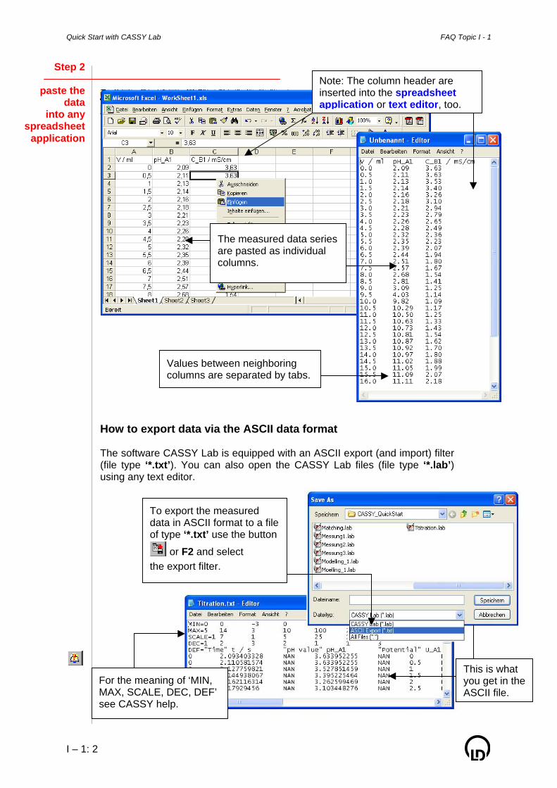
How to export data via the ASCII data format The software CASSY Lab is equipped with an ASCII export (and import) filter (file type ‘*.txt’). You can also open the CASSY Lab files (file type ‘*.lab’) using any text editor.

Step 2

paste thedata

into anyspreadsheet

application

Note: The column header are inserted into the spreadsheet application or text editor, too.

The measured data series are pasted as individual columns.

Values between neighboring columns are separated by tabs.

To export the measured data in ASCII format to a file of type ‘*.txt’ use the button or F2 and select the export filter.

For the meaning of ‘MIN, MAX, SCALE, DEC, DEF’ see CASSY help.

This is what you get in the ASCII file.

FAQ Topic II - 1 Quick Start with CASSY Lab

II – 1: 1

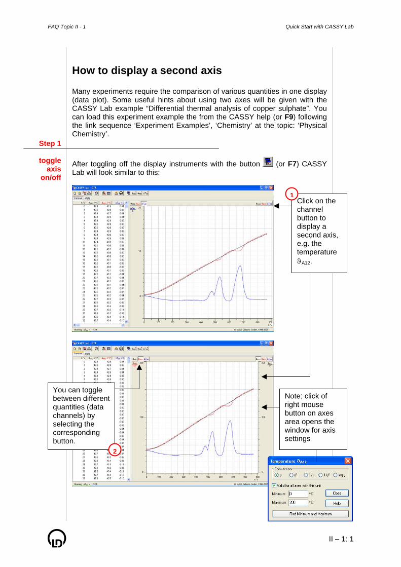
How to display a second axis Many experiments require the comparison of various quantities in one display (data plot). Some useful hints about using two axes will be given with the CASSY Lab example “Differential thermal analysis of copper sulphate”. You can load this experiment example the from the CASSY help (or F9) following the link sequence ‘Experiment Examples’, ‘Chemistry’ at the topic: ‘Physical Chemistry’.

After toggling off the display instruments with the button (or F7) CASSY Lab will look similar to this:

Step 1

toggleaxis

on/off

Click on the channel button to display a second axis,e.g. the temperature ϑA12.

You can toggle between differentquantities (data channels) by selecting the corresponding button.

Note: click of right mouse button on axes area opens the window for axis settings

1

2

Quick Start with CASSY Lab FAQ Topic II - 1

II – 1: 2

Often the selected axis (e.g. the right y-axis) of a quantity has to be rescaled and shifted in respect to the other axis (i.e. the left y-axis). In this example the difference temperature ∆T shall be shifted in respect to the temperatures ϑA12 and ϑA13.

For generating a stacked plot of measurements using the MCA-box (524 058) see FAQ Topic II – 2.

Step 2

shiftand

scaleaxis

shift the y-axis origin by clicking on the axis area, drag the axis and drop it at your required position.

You might want to rescale the axes to scale the various plots − e.g. here the black (ϑA12) and red curve (ϑA13) in respect to blue curve (∆T). A click of right mouse button on axes area opens a dialog window for the scaling of the axis of ϑA12 and ϑA13.


II – 2: 1

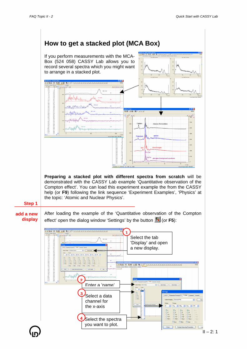
How to get a stacked plot (MCA Box) If you perform measurements with the MCA-Box (524 058) CASSY Lab allows you to record several spectra which you might want to arrange in a stacked plot.

Preparing a stacked plot with different spectra from scratch will be demonstrated with the CASSY Lab example ‘Quantitative observation of the Compton effect’. You can load this experiment example the from the CASSY help (or F9) following the link sequence ‘Experiment Examples’, ‘Physics’ at the topic: ‘Atomic and Nuclear Physics’. After loading the example of the ‘Quantitative observation of the Compton effect’ open the dialog window ‘Settings’ by the button (or F5):

Step 1

add a newdisplay

Select the tab ’Display’ and open a new display.

Enter a ’name’

Select a data channel for the x-axis

1

2

3

Select the spectra you want to plot.

4


II – 2: 2

Step 2

you mightwant tochange

standardplot

settings

Click right mouse button in the display to change the graphic settings

Note: yon can add or remove spectra by dragging and dropping the channel buttons between the top bar and the axis symbols.

Step 3

changescaling

of y-axis

Click right mouse button here to chose appropriate Maximum and Minimum y-values.

Select here whether the y-axis scaling should be valid for all data channels.

1

2

Note: If you start the experiment from ‘Load settings’ the recorded spectra will be displayed like this (i.e. not stacked).


II – 2: 3

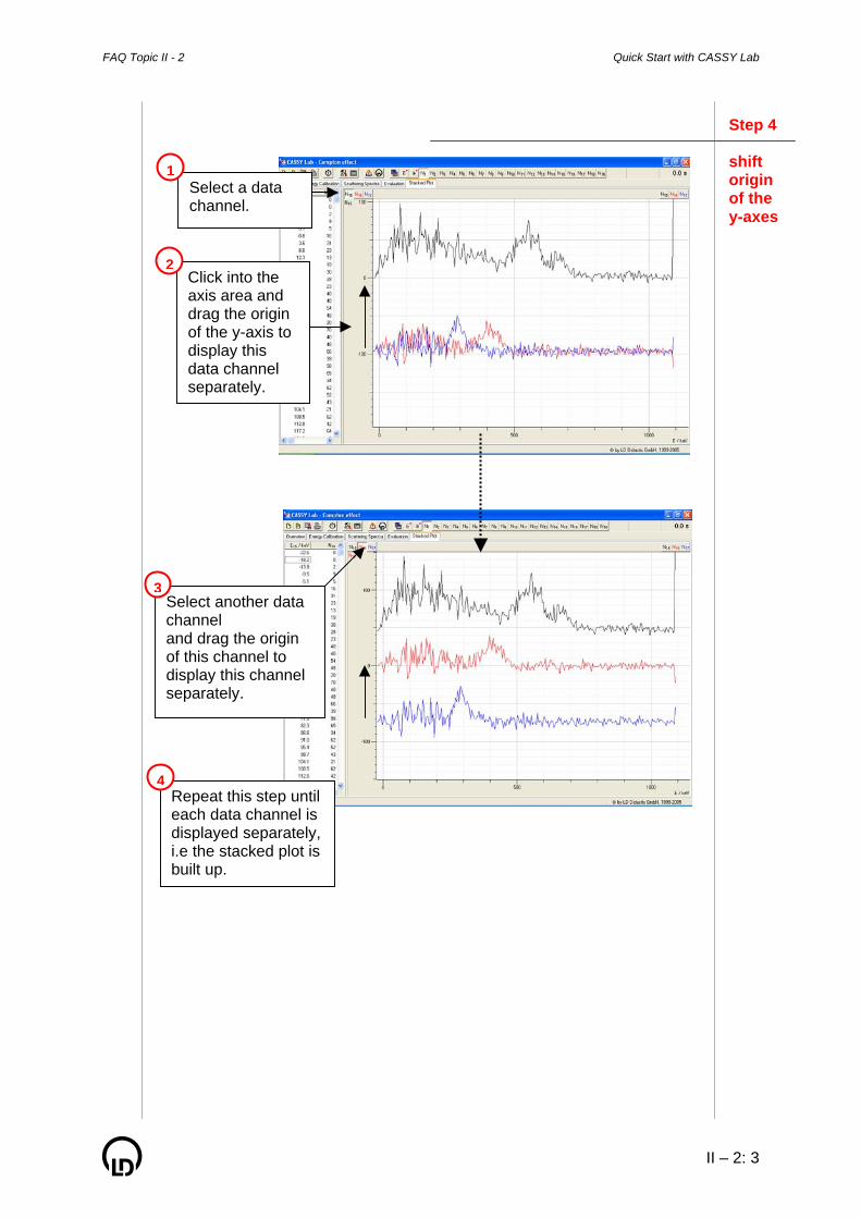
Step 4 shift origin of the y-axes

Click into the axis area and drag the origin of the y-axis to display this data channel separately.

Select a data channel.

1

2

Select another data channel and drag the origin of this channel to display this channel separately.

3

Repeat this step until each data channel is displayed separately, i.e the stacked plot is built up.

4


II – 2: 4

FAQ Topic III - 1 Quick Start with CASSY Lab

III – 1: 1

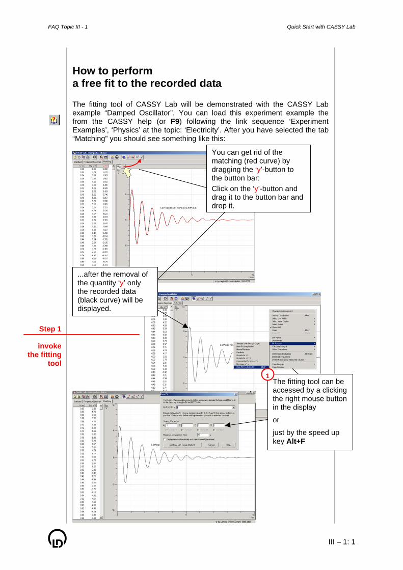
How to perform a free fit to the recorded data The fitting tool of CASSY Lab will be demonstrated with the CASSY Lab example “Damped Oscillator”. You can load this experiment example the from the CASSY help (or F9) following the link sequence ‘Experiment Examples’, ‘Physics’ at the topic: ‘Electricity’. After you have selected the tab “Matching” you should see something like this:

You can get rid of the matching (red curve) by dragging the ‘y’-button to the button bar: Click on the ‘y’-button and drag it to the button bar and drop it.

...after the removal of the quantity ‘y’ only the recorded data (black curve) will be displayed.

The fitting tool can be accessed by a clicking the right mouse button in the display

or

just by the speed up key Alt+F

1

Step 1

invokethe fitting

tool

Quick Start with CASSY Lab FAQ Topic III - 1

III – 1: 2

After invoking the fitting tool the proper fit model (mathematical formula) has to be selected. In the case of the damped oscillator you can choose a predefined function.

Remark: The sine function has been chosen according the Trigger Settings in the ‘Measurement Parameter’ menu.

Remark: The fit algorithm depends crucially on the starting value of the frequency. The frequency can be easily determined by Fourier Transformation.

Step 2

selectthe

fit model

You may enter the fit function here

or

you may select a predefined function from the pull down menu

2

Step 3

enterappropriate

startingvalues for

the fitparameters

)DtCsin(eAU Bt

+⋅⋅⋅=−

Enter meaningful estimate values for the fit parameters A, B, C, D

3

For the example here: A ~ 5 V (Amplitude) B ~ 1E-3 s (decay constant) C ~ 1E+3 Hz (frequency) D ~ 0 (phase shift)

Note: In this example the value D is kept constant.


III – 1: 3

In some cases, you may wish to mark a particular curve section for which the evaluation function has to perform a calculation.

To mark a curve section, hold down the left mouse button and drag the pointer to the end of the curve section. Alternatively, you can also click on the starting and end points. During marking, the marked curve section is displayed in green.

Step 4 select the data range for the fit

Select whether the fit result shall be put in a new channel

or

treated as a usual evaluation.

Continue with the button ‘Range Marking’ to mark a curve section.

4

Hint

You may display the result of the fit (shown in the status line) by using the speed up key Alt+T.


III – 1: 4

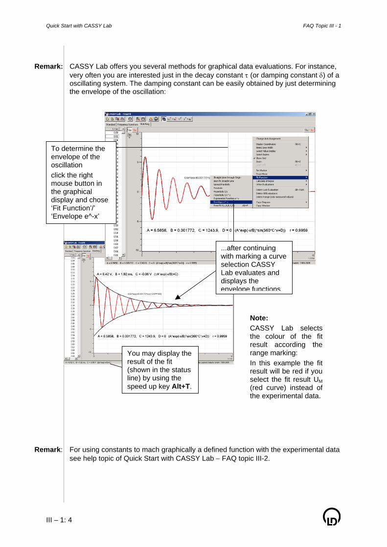
Remark: CASSY Lab offers you several methods for graphical data evaluations. For instance, very often you are interested just in the decay constant τ (or damping constant δ) of a oscillating system. The damping constant can be easily obtained by just determining the envelope of the oscillation:

Remark: For using constants to mach graphically a defined function with the experimental data see help topic of Quick Start with CASSY Lab − FAQ topic III-2.

To determine the envelope of the oscillation click the right mouse button in the graphical display and chose ‘Fit Function’/’ ‘Envelope e^-x’

...after continuing with marking a curve selection CASSY Lab evaluates and displays the envelope functions.

You may display the result of the fit (shown in the status line) by using the speed up key Alt+T.

Note: CASSY Lab selectsthe colour of the fitresult according therange marking: In this example the fitresult will be red if youselect the fit result UM(red curve) instead ofthe experimental data.


III – 2: 1

How to define formula − displaying a second axis Some quantities cannot be measured directly using CASSY. However, CASSY allows you define new quantities. One possibility is to use formulas.

Note: The temperature range determines the axis settings of a display when dragging a formula (e.g. ‘New Quantity’) into a display. For Axis settings see CASSY help. For entering formula see CASSY help

Step 1

definethe

newformula

Click on the tool box button and open the dialog window ‘Settings’

1

Select the tab ‘Parameter/Formula/FFT’ and click on the Button ‘New Quantity’

2

Enter

name Temperature

formula &JA11+273.15 K

symbol T

unit K

and desired

temperature range

to displayed

3


III – 2: 2

There are many reasons to depict the recoded data values differently. CASSY Lab allows you to display your data values in many different ways.

As a simple example the measured temperature values shall now be displayed at the same time on a centigrade scale and a Kelvin scale. To display a Kelvin scale on the same plot you first have to define first a new quantity. After displaying the formula in the graphical display a second axis can be displayed on the right margin of the display just by clicking on the button of the new quantity temperature ‘T’:

Remark: CASSY Lab automatically selects the colour settings. The colour of the symbols in the plot correspond to the colour of the buttons.

Step 2

displayinga second

axis

Click on the button ‘T’ of the ‘New Quantity’ Temperature to add an new axis on the right hand side of the plot.

4


III – 3: 1

How to use constants and formula for data matching There are several ways to define new quantities. One possibility is define a new quantity as a constant. Together with the use of formula (FAQ topic III-2) they allow the matching of a mathematical function to the experimental data in an elegant way.

To demonstrate the usage of constants and formula the CASSY Lab example “Damped Oscillator” will be used. You can load this experiment example the from the CASSY help (or F9) following the link sequence ‘Experiment Examples’, ‘Physics’ at the topic: ‘Electricity’. After you have selected the tab “Matching” you should see something like this:

According to theory a damped oscillation of the voltage U can be described by the following function with the parameters U0 (amplitude), τ (damping constant), ν (frequency) and phase shift ϕ.

Step 1

definea

newconstant

You can get rid of the matching (red curve) by dragging the ‘y’-button to the button bar: Click on the ‘y’-button and drag it to the button bar and drop it.

...after the removal of the quantity ‘y’ only the recorded data (black curve) will be displayed.

)t360sin(eU)t(Ut

0 ϕ+⋅ν⋅⋅⋅= τ−


III – 3: 2

For a given experimental data set (black curve) all these parameters are constant. As a first step you have to define these constants. In the following the procedure of defining new constants in CASSY Lab will be demonstrated for the amplitude U0.

Invoke the dialog window for ‘Settings’ by clicking

on the tool box button

and define a ‘New Quantity’ as constant.

1

enter the name2

For the difference between constants, parameters and formula see CASSY help

enter the symbol

Note: ‘_’ underscore gives index down the sign ‘^’ gives index up ‘&’ followed by a letter allows you to enter Greek letters.

You may set the constant to a certain initial value

3

4

enter the unit of the constant here

5 define the range for the instrument here

6

chose appropriate decimal places here

7

The new constants are added to the speed buttons on the top bar.

‘&j’ displays ‘ϕ’

Step 1

definea

newconstant


III – 3: 3

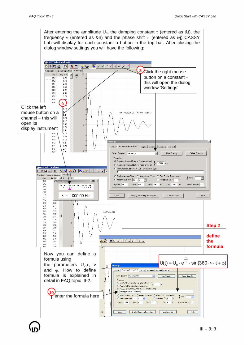
After entering the amplitude U0, the damping constant τ (entered as &t), the frequency ν (entered as &n) and the phase shift ϕ (entered as &j) CASSY Lab will display for each constant a button in the top bar. After closing the dialog window settings you will have the following:

Now you can define a formula using the parameters U0,τ, ν and ϕ. How to define formula is explained in detail in FAQ topic III-2.:

Click the right mouse button on a constant − this will open the dialog window ‘Settings’

Click the left mouse button on a channel − this will open its display instrument

8

9

Step 2 define the formula

enter the formula here10

)t360sin(eU)t(Ut

0 ϕ+⋅ν⋅⋅⋅= τ−


III – 3: 4

Step 3

changeconstants

untilmatching

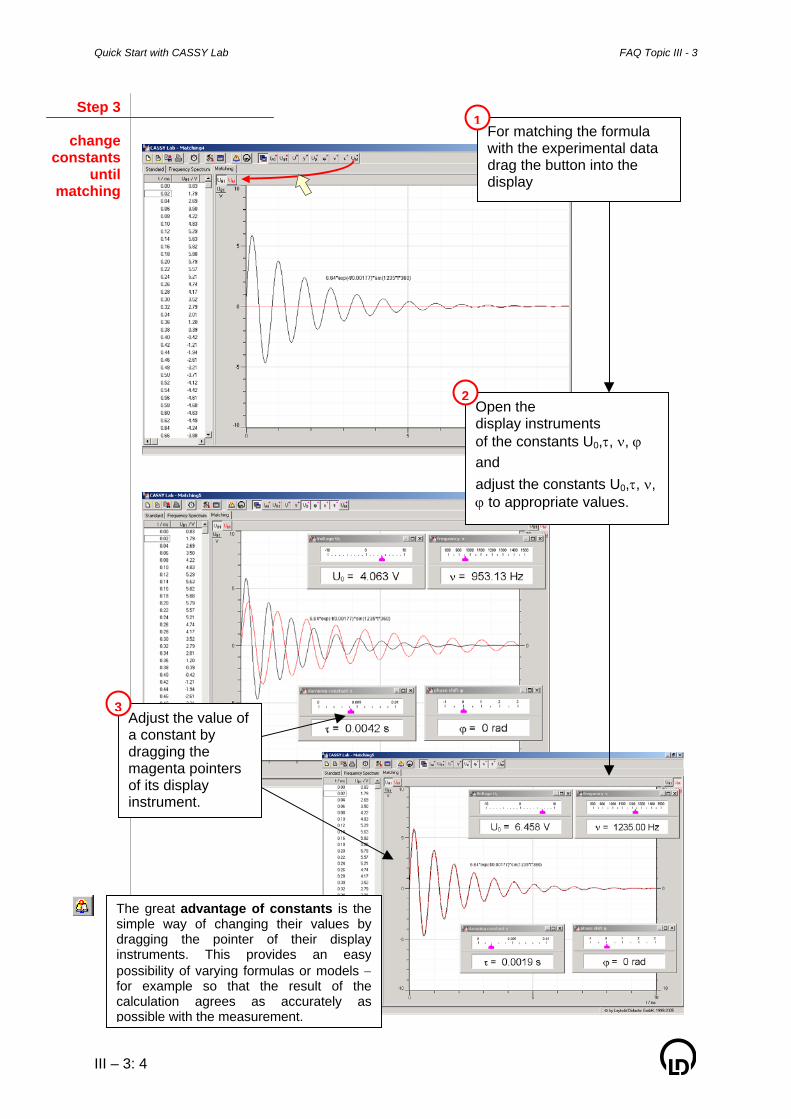
For matching the formula with the experimental data drag the button into the display

1

Open the display instruments of the constants U0,τ, ν, ϕ and adjust the constants U0,τ, ν, ϕ to appropriate values.

2

Adjust the value of a constant by dragging the magenta pointers of its display instrument.

3

The great advantage of constants is thesimple way of changing their values bydragging the pointer of their displayinstruments. This provides an easypossibility of varying formulas or models −for example so that the result of thecalculation agrees as accurately aspossible with the measurement.


III – 4: 1

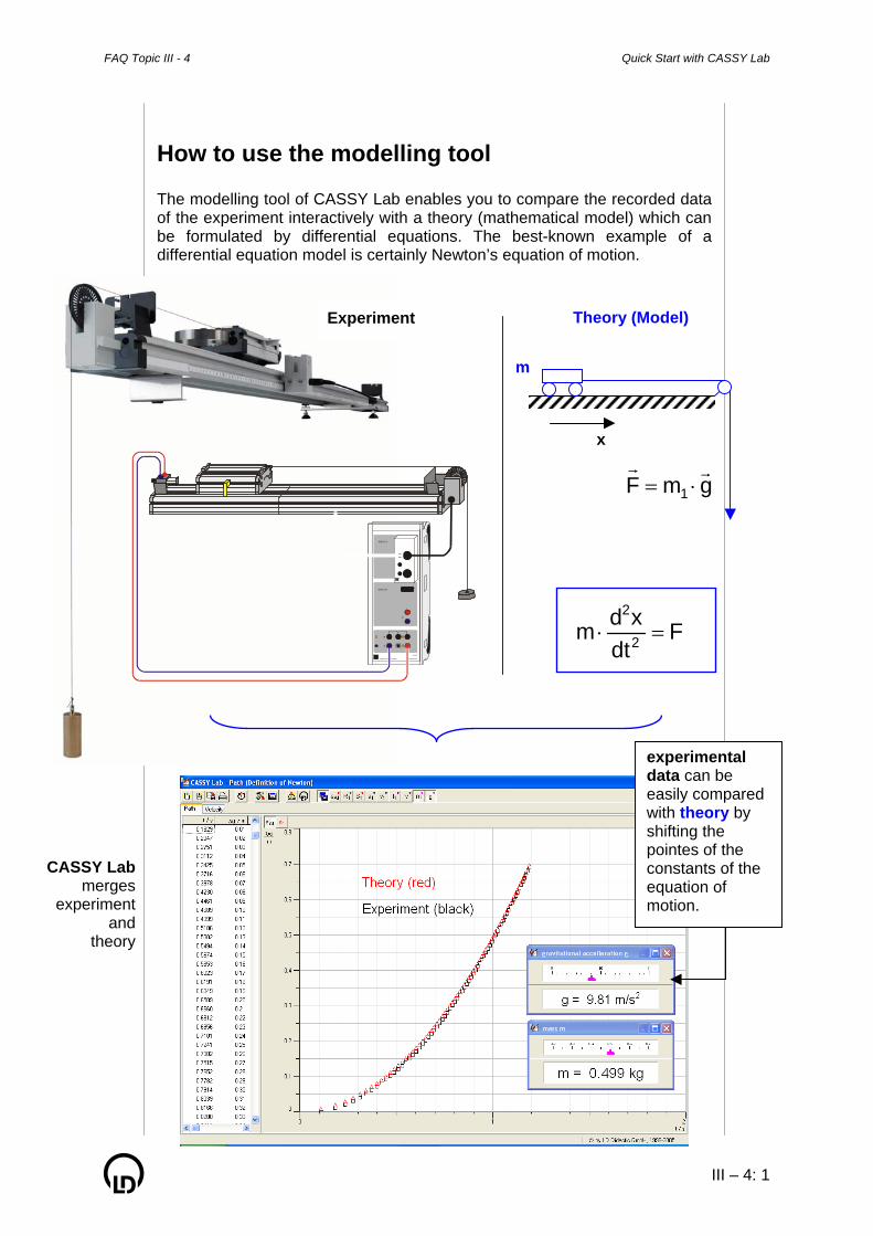
How to use the modelling tool The modelling tool of CASSY Lab enables you to compare the recorded data of the experiment interactively with a theory (mathematical model) which can be formulated by differential equations. The best-known example of a differential equation model is certainly Newton’s equation of motion.

F

dtxdm 2

2

=⋅

LEYBOLD DIDACT IC GMBH

S

R

SENSOR-CASSY

524 010

U

INPUT B

INPUT A

U

I

x

m

Theory (Model) Experiment

gmF 1

rr⋅=

experimental data can be easily compared with theory by shifting the pointes of the constants of the equation of motion.

CASSY Labmerges

experimentand

theory


III – 4: 2

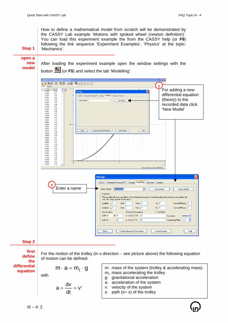
How to define a mathematical model from scratch will be demonstrated by the CASSY Lab example ‘Motions with spoked wheel (newton definition)’. You can load this experiment example the from the CASSY help (or F9) following the link sequence ‘Experiment Examples’, ‘Physics’ at the topic: ‘Mechanics’. After loading the experiment example open the window settings with the

button (or F5) and select the tab ‘Modelling’.

For the motion of the trolley (in x-direction − see picture above) the following equation of motion can be defined:

gmam 1 ⋅=⋅

with

Step 1

open anew

model

For adding a new differential equation (theory) to the recorded data click ‘New Model’

1

Enter a name 2

Step 2

firstdefine

thedifferential

equation

'vdtdva ==

m: mass of the system (trolley & accelerating mass)m1: mass accelerating the trolley g: gravitational acceleration a: acceleration of the system v: velocity of the system s: path (s= x) of the trolley


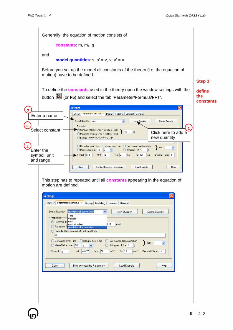
III – 4: 3

Generally, the equation of motion consists of constants: m, m1, g and model quantities: s, s’ = v, v, v’ = a. Before you set up the model all constants of the theory (i.e. the equation of motion) have to be defined. To define the constants used in the theory open the window settings with the

button (or F5) and select the tab ‘Parameter/Formula/FFT’.

This step has to repeated until all constants appearing in the equation of motion are defined.

Step 3 define the constants

Select constant Click here to add a new quantity

1

Enter a name 2

3

Enter the symbol, unit and range

4


III – 4: 4

After the definition of the constants the model quantities (here path and velocity) have to be defined.

To define the model of the theory open the window settings with the button (or F5) and select the tab ‘Modelling’.

Enter the equation of motion (differential equation). The differential equation may depend on constants which have to be defined first. To solve the equation of motion numerically, CASSY Lab needs to have the initial values of the two model quantities.

Note: Further information about various settings of the menu modelling can be found in the CASSY help ‘Settings – Modelling’. Use the index of the help menu and search for ‘Modelling’ to open this help topic.

Step 4

definethe

modelquantities

Enter the symbol of the two model quantities Select an appropriate range, e.g. like used in the display ‘Path’ and ‘Velocity’, respectively.

Enter a name

Select type of differential equation

Enter the equation of motion

Step 5

entermodel

Step 6

enterinitial

values

Note: Different initial values may be achieved by using appropriate trigger settings in the menu ’Measurement Parameters’

1

2

3

4


III – 4: 5

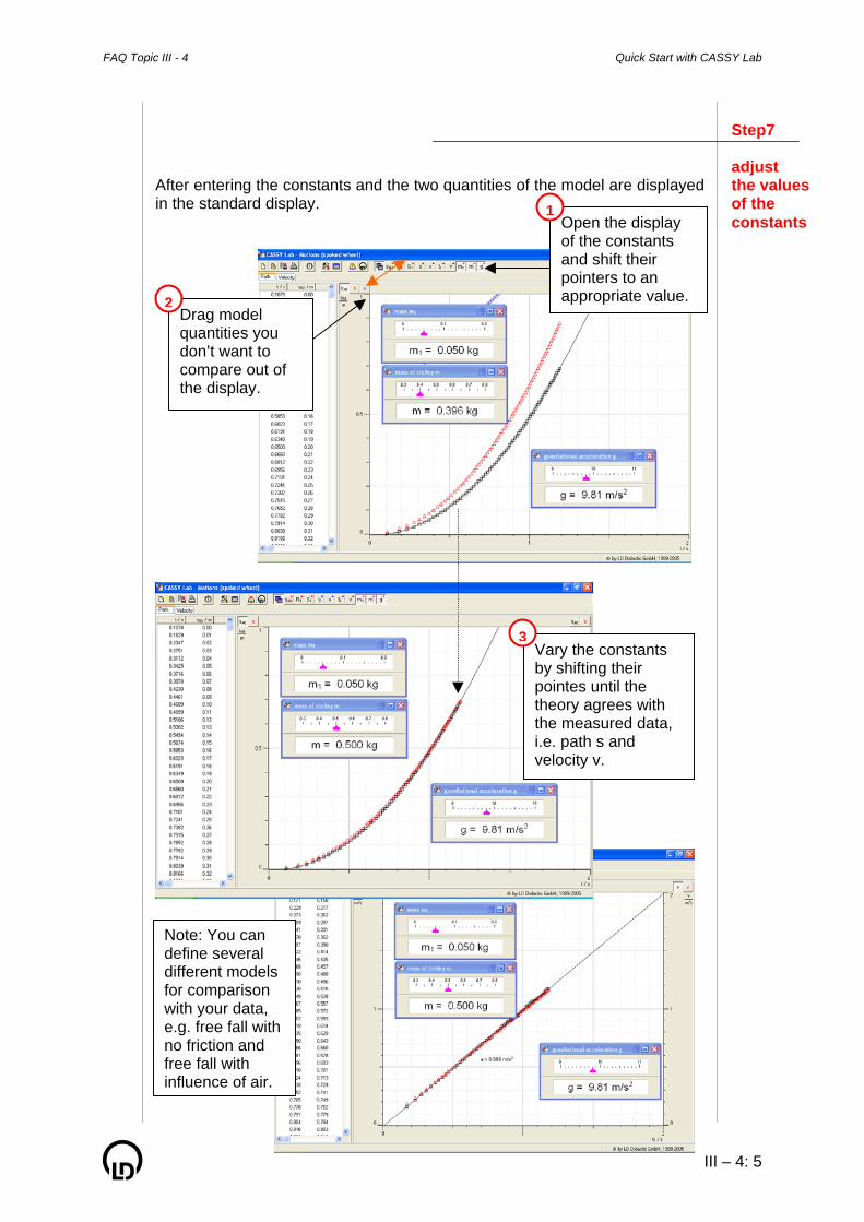
After entering the constants and the two quantities of the model are displayed in the standard display.

Step7 adjust the valuesof the constantsOpen the display

of the constants and shift their pointers to an appropriate value.

Drag model quantities you don’t want to compare out of the display.

1

2

Vary the constants by shifting their pointes until the theory agrees with the measured data, i.e. path s and velocity v.

3

Note: You can define several different models for comparison with your data, e.g. free fall with no friction and free fall with influence of air.


III – 4: 6

cassy lab - school-labs.com · faq topic ii - 2 quick start with cassy lab ii – 2: 1 how to get a...

Documents