Categorical Data Analysis1

STA 312: Fall 2012

1See last slide for copyright information.1 / 1

Variables and Cases

I There are n cases (people, rats, factories, wolf packs) in adata set.

I A variable is a characteristic or piece of information thatcan be recorded for each case in the data set.

I For example cases could be patients in a hospital, andvariables could be Age, Sex, Diagnosis, Have family doctor(Yes-No), Family history of heart disease (Yes-No), etc.

2 / 1

Variables can be Categorical, or Continuous

I Categorical: Gender, Diagnosis, Job category, Have familydoctor, Family history of heart disease, 5-year survival(Y-N)

I Some categories are ordered (birth order, health status)

I Continuous: Height, Weight, Blood pressure

I Some questions:I Are all normally distributed variables continuous?I Are all continuous variables quantitative?I Are all quantitative variables continuous?I Are there really any data sets with continuous variables?

3 / 1

Variables can be Explanatory, or Response

I Explanatory variables are sometimes called “independentvariables.”

I The x variables in regression are explanatory variables.

I Response variables are sometimes called “dependentvariables.”

I The Y variable in regression is the response variable.

I Sometimes the distinction is not useful: Does each twin getcancer, Yes or No?

4 / 1

Our main interest is in categorical variables

I Especially categorical response variables

I In ordinary regression, outcomes are normally distributed,and so continuous.

I But often, outcomes of interest are categoricalI Buy the product, or notI Marital status 5 years after graduationI Survive the operation, or not.

I Ordered categorical response variables, too: for examplehighest level of hockey ever played.

5 / 1

DistributionsWe will mostly use

I Bernoulli

I Binomial

I Multinomial

I Poisson

6 / 1

The Poisson processWhy the Poisson distribution is such a useful model for count data

I Events happening randomly in space or time

I Independent increments

I For a small region or interval,I Chance of 2 or more events is negligibleI Chance of an event roughly proportional to the size of the

region or interval

I Then (solve a system of differential equations), theprobability of observing x events in a region of size t is

e−λt(λt)x

x!for x = 0, 1, . . .

7 / 1

Poisson process examplesSome variables that have a Poisson distribution

I Calls coming in to an emergency number

I Customers arriving in a given time period

I Number of raisins in a loaf of raisin bread

I Number of bomb craters in a region after a bombing raid,London WWII

I In a jar of peanut butter . . .

8 / 1

Steps in the process of statistical analysisOne possible approach

I Consider a fairly realistic example or problem

I Decide on a statistical model

I Perhaps decide sample size

I Acquire data

I Examine and clean the data; generate displays anddescriptive statistics

I Estimate parameters, perhaps by maximum likelihood

I Carry out tests, compute confidence intervals, or both

I Perhaps re-consider the model and go back to estimation

I Based on the results of inference, draw conclusions aboutthe example or problem

9 / 1

Coffee taste test

A fast food chain is considering a change in the blend of coffeebeans they use to make their coffee. To determine whether theircustomers prefer the new blend, the company plans to select arandom sample of n = 100 coffee-drinking customers and askthem to taste coffee made with the new blend and with the oldblend, in cups marked “A” and “B.” Half the time the newblend will be in cup A, and half the time it will be in cup B.Management wants to know if there is a difference in preferencefor the two blends.

10 / 1

Statistical model

Letting π denote the probability that a consumer will choose thenew blend, treat the data Y1, . . . , Yn as a random sample from aBernoulli distribution. That is, independently for i = 1, . . . , n,

P (yi|π) = πyi(1− π)1−yi

for yi = 0 or yi = 1, and zero otherwise.

Note that Y =∑n

i=1 Yi is the number of consumers who choosethe new blend. Because Y ∼ B(n, π), the whole experimentcould also be treated as a single observation from a Binomial.

11 / 1

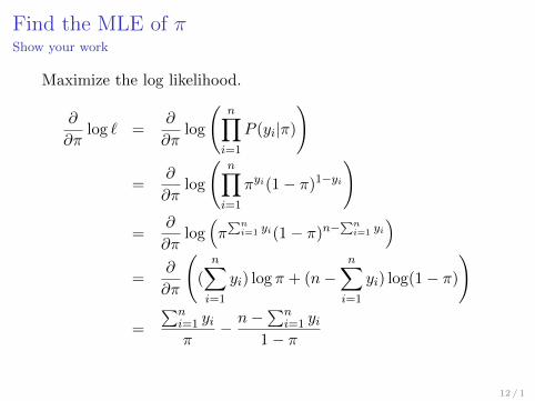
Find the MLE of πShow your work

Maximize the log likelihood.

∂

∂πlog ` =

∂

∂πlog

(n∏i=1

P (yi|π)

)

=∂

∂πlog

(n∏i=1

πyi(1− π)1−yi

)

=∂

∂πlog(π∑ni=1 yi(1− π)n−

∑ni=1 yi

)=

∂

∂π

((

n∑i=1

yi) log π + (n−n∑i=1

yi) log(1− π)

)

=

∑ni=1 yiπ

−n−

∑ni=1 yi

1− π

12 / 1

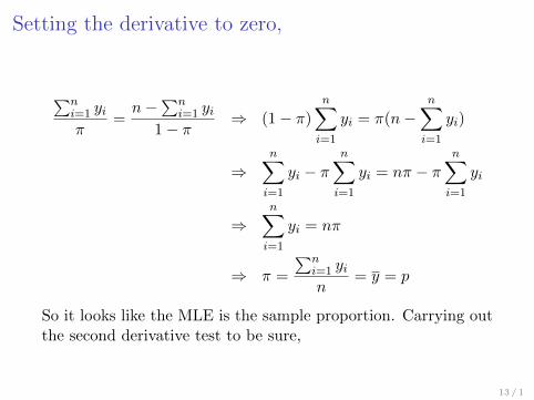
Setting the derivative to zero,

∑ni=1 yiπ

=n−

∑ni=1 yi

1− π⇒ (1− π)

n∑i=1

yi = π(n−n∑i=1

yi)

⇒n∑i=1

yi − πn∑i=1

yi = nπ − πn∑i=1

yi

⇒n∑i=1

yi = nπ

⇒ π =

∑ni=1 yin

= y = p

So it looks like the MLE is the sample proportion. Carrying outthe second derivative test to be sure,

13 / 1

Second derivative test

∂2 log `

∂π2=

∂

∂π

(∑ni=1 yiπ

−n−

∑ni=1 yi

1− π

)=−∑n

i=1 yiπ2

−−−n−

∑ni=1 yi

(1− π)2

= −n(

1− y(1− π)2

+y

π2

)< 0

Concave down, maximum, and π̂ = y = p.

14 / 1

Numerical estimate

Suppose 60 of the 100 consumers prefer the new blend. Give apoint estimate the parameter π. Your answer is a number.

> p = 60/100; p

[1] 0.6

15 / 1

Carry out a test to answer the questionIs there a difference in preference for the two blends?

Start by stating the null hypothesis

I H0 : π = 0.50

I H1 : π 6= 0.50

I A case could be made for a one-sided test, but we’ll stickwith two-sided.

I α = 0.05 as usual.

I Central Limit Theorem says π̂ = Y is approximatelynormal with mean π and variance π(1−π)

n .

16 / 1

Several valid test statistics for H0 : π = π0 are availableTwo of them are

Z1 =

√n(p− π0)√π0(1− π0)

and

Z2 =

√n(p− π0)√p(1− p)

What is the critical value? Your answer is a number.

> alpha = 0.05

> qnorm(1-alpha/2)

[1] 1.959964

17 / 1

Calculate the test statistic(s)and the p-value(s)

> pi0 = .5; p = .6; n = 100

> Z1 = sqrt(n)*(p-pi0)/sqrt(pi0*(1-pi0)); Z1

[1] 2

> pval1 = 2 * (1-pnorm(Z1)); pval1

[1] 0.04550026

>

> Z2 = sqrt(n)*(p-pi0)/sqrt(p*(1-p)); Z2

[1] 2.041241

> pval2 = 2 * (1-pnorm(Z2)); pval2

[1] 0.04122683

18 / 1

ConclusionsI Do you reject H0? Yes, just barely.I Isn’t the α = 0.05 significance level pretty arbitrary? Yes,

but if people insist on a Yes or No answer, this is what yougive them.

I What do you conclude, in symbols? π 6= 0.50. Specifically,π > 0.50.

I What do you conclude, in plain language? Your answer is astatement about coffee. More consumers prefer the newblend of coffee beans.

I Can you really draw directional conclusions when all youdid was reject a non-directional null hypothesis? Yes.Decompose the two-sided size α test into two one-sidedtests of size α/2. This approach works in general.

It is very important to state directional conclusions, and statethem clearly in terms of the subject matter. Say whathappened! If you are asked state the conclusion in plainlanguage, your answer must be free of statistical mumbo-jumbo.

19 / 1

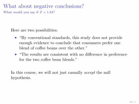
What about negative conclusions?What would you say if Z = 1.84?

Here are two possibilities.

I “By conventional standards, this study does not provideenough evidence to conclude that consumers prefer oneblend of coffee beans over the other.”

I “The results are consistent with no difference in preferencefor the two coffee bean blends.”

In this course, we will not just casually accept the nullhypothesis.

20 / 1

Confidence IntervalsApproximately for large n,

1− α ≈ Pr{−zα/2 < Z < zα/2}

= Pr

{−zα/2 <

√n(p− π)√p(1− p)

< zα/2

}

= Pr

{p− zα/2

√p(1− p)

n< π < p+ zα/2

√p(1− p)

n

}

I Could express this as p± zα/2√

p(1−p)n

I zα/2

√p(1−p)n is sometimes called the margin of error.

I If α = 0.05, it’s the 95% margin of error.

21 / 1

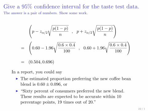
Give a 95% confidence interval for the taste test data.The answer is a pair of numbers. Show some work.

(p− zα/2

√p(1− p)

n, p+ zα/2

√p(1− p)

n

)

=

(0.60− 1.96

√0.6× 0.4

100, 0.60 + 1.96

√0.6× 0.4

100

)

= (0.504, 0.696)

In a report, you could say

I The estimated proportion preferring the new coffee beanblend is 0.60± 0.096, or

I “Sixty percent of consumers preferred the new blend.These results are expected to be accurate within 10percentage points, 19 times out of 20.”

22 / 1

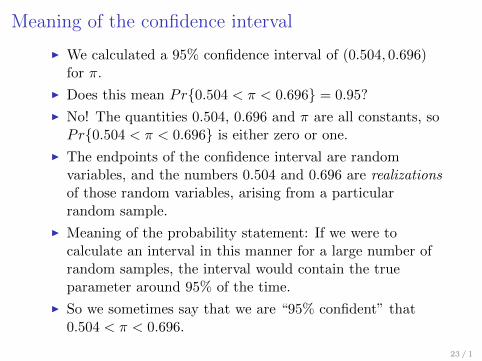
Meaning of the confidence interval

I We calculated a 95% confidence interval of (0.504, 0.696)for π.

I Does this mean Pr{0.504 < π < 0.696} = 0.95?

I No! The quantities 0.504, 0.696 and π are all constants, soPr{0.504 < π < 0.696} is either zero or one.

I The endpoints of the confidence interval are randomvariables, and the numbers 0.504 and 0.696 are realizationsof those random variables, arising from a particularrandom sample.

I Meaning of the probability statement: If we were tocalculate an interval in this manner for a large number ofrandom samples, the interval would contain the trueparameter around 95% of the time.

I So we sometimes say that we are “95% confident” that0.504 < π < 0.696.

23 / 1

Confidence intervals (regions) correspond to testsRecall Z1 =

√n(p−π0)√π0(1−π0)

and Z2 =√n(p−π0)√p(1−p)

.

From the derivation of the confidence interval,

−zα/2 < Z2 < zα/2

if and only if

p− zα/2

√p(1− p)

n< π0 < p+ zα/2

√p(1− p)

n

I So the confidence interval consists of those parametervalues π0 for which H0 : π = π0 is not rejected.

I That is, the null hypothesis is rejected at significance levelα if and only if the value given by the null hypothesis isoutside the (1− α)× 100% confidence interval.

I There is a confidence interval corresponding to Z1 too.Maybe it’s better – See Chapter 1.

I In general, any test can be inverted to obtain a confidenceregion.

24 / 1

Selecting sample size

I Where did that n = 100 come from?

I Probably off the top of someone’s head.

I We can (and should) be more systematic.

I Sample size can be selectedI To achieve a desired margin of errorI To achieve a desired statistical powerI In other reasonable ways

25 / 1

Power

The power of a test is the probability of rejecting H0 when H0

is false.

I More power is good.

I Power is not just one number. It is a function of theparameter.

I Usually,I For any n, the more incorrect H0 is, the greater the power.I For any parameter value satisfying the alternative

hypothesis, the larger n is, the greater the power.

26 / 1

Statistical power analysisTo select sample size

I Pick an effect you’d like to be able to detect – a parametervalue such that H0 is false. It should be just over theboundary of interesting and meaningful.

I Pick a desired power, a probability with which you’d like tobe able to detect the effect by rejecting the null hypothesis.

I Start with a fairly small n and calculate the power.Increase the sample size until the desired power is reached.

There are two main issues.

I What is an “interesting” or “meaningful” parameter value?

I How do you calculate the probability of rejecting H0?

27 / 1

Calculating power for the test of a single proportionTrue parameter value is π

Z1 =

√n(p− π0)√π0(1− π0)

Power = 1− Pr{−zα/2 < Z1 < zα/2}

= 1− Pr{−zα/2 <

√n(p− π0)√π0(1− π0)

< zα/2

}= . . .

= 1− Pr{√

n(π0 − π)√π(1− π)

− zα/2

√π0(1− π0)

π(1− π)<

√n(p− π)√π(1− π)

<

√n(π0 − π)√π(1− π)

+ zα/2

√π0(1− π0)

π(1− π)

}

≈ 1− Pr{√

n(π0 − π)√π(1− π)

− zα/2

√π0(1− π0)

π(1− π)< Z <

√n(π0 − π)√π(1− π)

+ zα/2

√π0(1− π0)

π(1− π)

}

= 1− Φ

(√n(π0 − π)√π(1− π)

+ zα/2

√π0(1− π0)

π(1− π)

)+ Φ

(√n(π0 − π)√π(1− π)

− zα/2

√π0(1− π0)

π(1− π)

),

where Φ(·) is the cumulative distribution function of thestandard normal.

28 / 1

An R function to calculate approximate powerFor the test of a single proportion

Power = 1− Φ

(√n(π0 − π)√π(1− π)

+ zα/2

√π0(1− π0)

π(1− π)

)+ Φ

(√n(π0 − π)√π(1− π)

− zα/2

√π0(1− π0)

π(1− π)

)

Z1power = function(pi,n,pi0=0.50,alpha=0.05)

{

a = sqrt(n)*(pi0-pi)/sqrt(pi*(1-pi))

b = qnorm(1-alpha/2) * sqrt(pi0*(1-pi0)/(pi*(1-pi)))

Z1power = 1 - pnorm(a+b) + pnorm(a-b)

Z1power

} # End of function Z1power

29 / 1

Some numerical examples

> Z1power(0.50,100)

[1] 0.05

>

> Z1power(0.55,100)

[1] 0.168788

> Z1power(0.60,100)

[1] 0.5163234

> Z1power(0.65,100)

[1] 0.8621995

> Z1power(0.40,100)

[1] 0.5163234

> Z1power(0.55,500)

[1] 0.6093123

> Z1power(0.55,1000)

[1] 0.8865478

30 / 1

Find smallest sample size needed to detect π = 0.55 asdifferent from π0 = 0.50 with probability at least 0.80

> samplesize = 50

> power=Z1power(pi=0.55,n=samplesize); power

[1] 0.1076602

> while(power < 0.80)

+ {

+ samplesize = samplesize+1

+ power = Z1power(pi=0.55,n=samplesize)

+ }

> samplesize; power

[1] 783

[1] 0.8002392

31 / 1

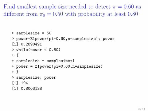
Find smallest sample size needed to detect π = 0.60 asdifferent from π0 = 0.50 with probability at least 0.80

> samplesize = 50

> power=Z1power(pi=0.60,n=samplesize); power

[1] 0.2890491

> while(power < 0.80)

+ {

+ samplesize = samplesize+1

+ power = Z1power(pi=0.60,n=samplesize)

+ }

> samplesize; power

[1] 194

[1] 0.8003138

32 / 1

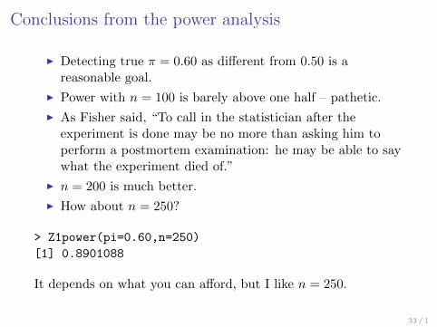
Conclusions from the power analysis

I Detecting true π = 0.60 as different from 0.50 is areasonable goal.

I Power with n = 100 is barely above one half – pathetic.

I As Fisher said, “To call in the statistician after theexperiment is done may be no more than asking him toperform a postmortem examination: he may be able to saywhat the experiment died of.”

I n = 200 is much better.

I How about n = 250?

> Z1power(pi=0.60,n=250)

[1] 0.8901088

It depends on what you can afford, but I like n = 250.

33 / 1

What is required of the scientistWho wants to select sample size by power analysis

The scientist must specify

I Parameter values that he or she wants to be able to detectas different from H0 value.

I Desired power (probability of detection)

It’s not always easy for the scientist to think in terms of theparameters of a statistical model.

34 / 1

Copyright Information

This slide show was prepared by Jerry Brunner, Department ofStatistics, University of Toronto. It is licensed under a CreativeCommons Attribution - ShareAlike 3.0 Unported License. Useany part of it as you like and share the result freely. TheLATEX source code is available from the course website:http://www.utstat.toronto.edu/∼brunner/oldclass/312f12

35 / 1