CAUSAL TRACKING CONTROL OF

A NON-MINIMUM PHASE

HIL TRANSMISSION TEST SYSTEM

Pengfei Wang

A thesis submitted for the degree of Doctor of Philosophy

University of Bath Department of Mechanical Engineering

December 2009

COPYRIGHT

Attention is drawn to the fact that copyright of this thesis rests with its author. This

copy of the thesis has been supplied on condition that anyone who consults it is

understood to recognise that its copyright rests with its author and no information

derived from it may be published without the prior written consent of the author.

This thesis may be made available for consultation within the University library and

maybe photocopied or lent to other libraries for the purposes of consultation.

Summary

The automotive industry has long relied on testing powertrain components in real

vehicles, which causes the development process to be slow and expensive. Therefore,

hardware in the loop (HIL) testing techniques are increasingly being adopted to

develop electronic control units (ECU) for engine and other components of a vehicle.

In this thesis, HIL testing system is developed to provide a laboratory testing

environment for continuously variable transmissions (CVTs). Two induction motors

were utilized to emulate a real engine and vehicle. The engine and vehicle models,

running in real-time, provide reference torque and speed signals for input and output

dynamometers, respectively. To design torque and speed tracking controllers, linear

models of the motor and drive systems were firstly identified from the test results.

Feedforward controllers were then designed according to the inverse dynamics of the

identified models. Because of the existence of unstable zeros in the model, design

effort was focused on the stability and causality of the inverse process. Digital

preview filters were formulated to approximate the stable inverse of unstable zeros as

part of the feedforward controller. Normally, future information of input trajectory is

required when implementing the digital preview filters, which makes the feedforward

controller non-causal. Since the engine and vehicle model require current

information to calculate the next output and no future value can be provided in

advance, the application of non-causal digital controllers was limited. A novel

method is proposed here to apply non-causal digital controllers causally. Robustness

of the controllers is also considered when the two motors are coupled and the gear

ratio between them was changed.

The proposed coupled control method was tested and verified experimentally by

using a manual gearbox before recommending its use for a CVT testing. A multi­

frequency test signal as well as simulation results of a whole vehicle model were

used as torque and speed demand signals in the experiments. A HIL testing case was

also presented. Frequency and time domain results showed the effectiveness of the

I

method under both testing procedures to fully compensate for the dynamics of both

actuators.

II

Acknowledgements

I would like to give my appreciation to everyone who has been supporting me in all

these three tough years.

Very special thanks to my supervisors Dr. Necip Sahinkaya and Dr. Sam Akehurst. I

can never finish my PhD without your expertise, guidance and patience.

Many thanks to the technicians for your assistance on the test rig.

谨以此论文献给我最亲爱的父母，你们的支持和信任永远是我最大的动力。

III

Contents

NOTATIONS................................................................................................ VII

CHAPTER 1 INTRODUCTION .................................................................. 1

1.1 CVT.................................................................................................................. 1

1.1.1 Introduction of CVT................................................................................. 1

1.1.2 Testing of CVT ........................................................................................ 6

1.2 Hardware in the Loop (HIL) Testing ............................................................... 7

1.3 HIL Test Facility for CVTs............................................................................ 10

1.3.1 Test Facility Architecture....................................................................... 10

1.3.2 Test Facility Components ...................................................................... 11

1.3.3 Control of Dynamometers...................................................................... 14

1.4 Feedforward Control ...................................................................................... 15

1.4.1 Control Scheme...................................................................................... 15

1.4.2 Inverse Feedforward Control ................................................................. 17

1.4.3 Stable Inversion of Non-minimum Phase Systems................................ 18

1.4.4 Comments on Stable Inversion Techniques........................................... 23

1.5 Thesis Scope .................................................................................................. 24

CHAPTER 2 SYSTEM IDENTIFICATION................................................ 25

2.1 Identification Method..................................................................................... 26

2.1.1 Least Squares Estimation ....................................................................... 26

2.1.2 Multi-Frequency Signal ......................................................................... 28

2.1.3 Statistical Analysis ................................................................................. 30

2.2 Identification Results ..................................................................................... 33

IV

2.2.1 Estimation of Inertia and Damping ........................................................ 34

2.2.2 Estimation of Motor and Drive System ................................................. 41

2.3 Transmission Delay in CAN Bus................................................................... 48

2.4 Model for Speed Control with CAN Bus Delay ............................................ 51

2.4.1 Simulink Model...................................................................................... 51

2.4.2 Estimated Transfer Function.................................................................. 56

CHAPTER 3 FEEDFORWARD TRACKING CONTROLLER................... 59

3.1 Digital Preview Filter..................................................................................... 59

3.1.1 Design of DPF........................................................................................ 60

3.1.2 Norm Optimization for DPF .................................................................. 62

3.2 Causal Design of DPF.................................................................................... 65

3.3 Causal Application of DPF to a Single Motor ............................................... 67

3.3.1 Output Dynamometer Speed Tracking Control ..................................... 67

3.3.2 Input Dynamometer Generated Torque Tracking Control..................... 75

3.4 Conclusions.................................................................................................... 80

CHAPTER 4 FEEDFORWARD CONTROLLER ROBUSTNESS............. 82

4.1 Gear Ratio Compensation of O/P Dynamometer Speed Control................... 83

4.1.1 Test with Neutral Gear ........................................................................... 84

4.1.2 Test with 1:1 Gear Ratio ........................................................................ 87

4.2 Compensation of Disturbance Torque for O/P Dynamometer....................... 90

4.3 Compensation of Inertia Torque for I/P Dynamometer ................................. 96

4.3.1 Test with Inertia Torque Compensator .................................................. 97

4.3.2 Test with additional PID controllers .................................................... 101

CHAPTER 5 TESTING WITH REAL TIME MODEL............................... 106

5.1 Engine and Vehicle model ........................................................................... 106

V

5.2 Testing with Simulation Results .................................................................. 107

5.3 HIL Testing .................................................................................................. 116

CHAPTER 6 CONCLUSIONS................................................................ 121

6.1 Conclusions.................................................................................................. 121

6.2 Future Work ................................................................................................. 122

REFERENCES .......................................................................................... 124

VI

Notations

A Vehicle frontal area

A Matrix as a function of

21, AA Matrices calculated from the weighting function w

Ak Amplitude of harmonic component

BI Combined damping ratio of input dynamometer and shaft

BM Motor damping ratio

BN Nominal damping ratio

BO Combined damping ratio of output dynamometer and shaft

C Vector of transfer function coefficients

CD Drag coefficient

D Number of preview steps required for feedforward controller

)( 1DPF z Transfer function of digital preview filter

)( 1zDPFA Transfer function of digital preview filter for gain compensation

)( 1 zDPF Transfer function of digital preview filter for phase compensation

F Complex measurement variable

FL Measurement vector used in the Least Square Estimation

tF Engine driving force

G(s) Continuous-time transfer function of the plant

(s)Gclose Continuous-time transfer function of closed loop speed control

( )_ sG DynoI Motor and drive system transfer function of input dynamometer

( )_ sG DynoO Motor and drive system transfer function of output dynamometer

(s)GPID Transfer function of PID controller

( )_ sG cmpRatio Transfer function of gear ratio compensator

(s)GSpeed Transfer function of output dynamometer speed control

VII

(s)GTorque Transfer function of input dynamometer torque control

)( 1zH Discrete-time transfer function of the plant

)( 1zH a Stable (acceptable) part of )( 1zH

)( 1zH Close Discrete-time equivalent of (s)Gclose with ZOH

)( 1 &

zH LM Discrete-time equivalent of ( )( ) __ sLsG DynoODynoO with ZOH

)( 1zH PID Discrete-time equivalent of (s)GPID with ZOH

)( 1zH Speed Discrete-time equivalent of (s)GSpeed with ZOH

)( 1zHTorque Discrete-time equivalent of (s)GTorque with ZOH

)( 1zH u Unstable (unacceptable) part of )( 1zH

J I Combined inertia of input dynamometer and shaft

J M Motor inertia

J N Nominal inertia

J O Combined inertia of output dynamometer and shaft

J Sh Shaft inertia

K Number of frequency components

( )&_ sL ShsDI Load transfer function of input dynamometer and shafts

( )_ sL DynoI Load transfer function of input dynamometer

( )_ sL ShaftI Load transfer function of input shaft

( )_ sL DynoO Load transfer function of output dynamometer

( )_ sL ShaftO Load transfer function of output shaft

N Number of preview steps for )( 1DPF z

P Number of unstable zeros in )( 1zH

2P1 , P Number of real and complex zeros in )( 1zH

Pk Ratio of power to the total power

)( 1Q z Transfer function of feedforward controller

R Relative order of the estimated transfer function )( nm

R 2 Goodness of fit measurement

R(s) Generic output signal

VIII

)( 1R z Ratio transfer function

gT Generated torque

mT Measured torque

sT Sampling time

Y (s) Generic output signal

Z Complex measurement vector for a single frequency

ZL Measurement matrix used in the Least Square Estimation

a Vehicle acceleration

ai Parameters for denominators of the estimated transfer function

bi Parameters for numerators of the estimated transfer function

e Residual

g Gravity acceleration

i, k Integers

m Order of the denominator of the estimated transfer function

vm Vehicle mass

n Order of the numerator of the estimated transfer function

p Number of data points

pk Power spectrum

q Number of estimated coefficients

r Plant input signal

cr Rolling resistance coefficient

s Laplace transform operator

v Residual degrees of freedom

vv Vehicle speed

w Weighting function

y Plant output signal

yd Desired signal

y f Delayed output signal

z Discrete z-transform operator

IX

zi Unstable zeros

( ,) Lagrange transfer function

α Vector of coefficients of DPFA

i Coefficients of DPFA

β Vector of constants

Covariance matrix

γ Vector of coefficients of zero phase filter

i Coefficients of zero phase filter

, Coefficients of R(z 1 )

Normalized frequency

1,2 Lower and upper limits of normalized frequency

Road gradient r

Lagrange multiplier

Air density

2 Mean Square Residual

Gear ratio between output and input dynamometers

k Phase of kth frequency component in SPHS signal

Frequency

0 Fundamental frequency

M Motor speed

(··) Derivatives

(¯) Complex conjugate

(^) Estimation

( )-1 Inverse

X

Chapter 1 Introduction

In this chapter, a general introduction to continuously variable transmissions (CVTs)

and hardware in the loop (HIL) testing techniques is presented as the background of

this research. To assist the CVT calibration and development processes, a HIL test

facility is developed in a laboratory environment using two electric motors as prime

movers and absorbers. The vital part in the HIL testing is to control the torque and

speed of these motors to track the engine torque and vehicle speed calculated from

the real-time simulation models. To achieve a perfect tracking, a feedforward control

is normally used, in addition to a feedback control. Inverse techniques for the design

of feedforward controllers are presented. Background on the concepts of minimum

and non-minimum phase systems is introduced, and stable inverse techniques for

non-minimum phase systems are reviewed. A scope of the thesis is also given at the

end of the chapter.

1.1 CVT

Currently, most vehicles use either conventional manual transmissions or automatic

transmissions configured with multiple planetary gear sets that use integral clutches

and bands to achieve discrete gear ratios. The way continuously variable

transmission (CVT) differs from manual and automatic transmissions is that the gear

ratio is not discretized and can thus be changed continuously between the minimum

and maximum values.

1.1.1 Introduction of CVT

Configuration of CVT

The most common configuration of CVTs applied in automotive industry is the

pushing metal belt CVT. The feature that characterizes this type of CVT is the

1

variable-diameter pulleys. Each pulley is made of two cones facing each other. A belt

rides in the groove between the two cones. The variable-diameter pulleys must

always come in pairs. One of the pulleys, known as the drive or primary pulley, is

connected to the crankshaft of the engine. The second pulley is called the driven or

secondary pulley which transfers energy to the vehicle driveshafts. The components

are shown in Figure 1-1.

Primary

Secondary

Primary

Secondary

Figure 1-1 Configuration of push belt CVT

The distance between the centres of the pulleys to where the belt makes contact in

the groove is known as the pitch radius, shown in Figure 1-1 as p and s. Since the

pulley centre distance is fixed and the belt length is constant, when the radius of one

pulley is increased, the radius of the other pulley must be decreased to keep the belt

tight. The force can be created from hydraulic pressure, centrifugal force or spring

tension to adjust the pulley haves. As the two pulleys change their radii relative to

one another, an infinite number of gear ratios is created from low to high and

everything in between.

There are also other configurations for CVT, such as toroidal CVTs [1,2] and

hydrostatic CVT [3,4]. Although different in components and configuration, all the

CVTs have the capability of changing the gear ratio continuously.

Function of CVT

The major advantage of CVT technology is that it allows the engine to operate in a

more fuel efficient manner. Unlike other transmissions which only allow a few

discrete gear ratios, CVT essentially enable an infinite number of ratios available

2

within a finite range, so the relationship between the speed of a vehicle, the

equivalent road load torque, and the engine speed and torque can be selected within a

continuous range. This gives the freedom to operate an engine at speeds that are not

fixed in relation to the vehicle speed. In addition, the use of electronic engine control

allows the engine torque output to be set by the control strategy rather than the driver.

When used together, these two features allow the driver’s power demand to be

implemented in the most advantageous manner. This has been traditionally

demonstrated as a means to optimise fuel economy by running the engine along a

line of minimum brake specific fuel consumption (BSFC), usually called an

economy line (E-line) [5], shown in Figure 1-2. There is another line (D-line) shown

in the figure, which will be further explained later.

Figure 1-2 Economic and dynamic operating line in engine map

The function of CVT is to make engine operate along the determined E-line to save

fuel, in dependent of vehicle speed. Figure 1-3 shows one way to generate the target

engine torque and target CVT ratio under the steady state operation. The engine

power demand was firstly calculated as the product of the target driving force and

vehicle speed, the intersection of iso-horsepower and the target engine operating line

(E-line) was selected as the ideal operating point defining the target engine torque

and engine speed for this desired driving force. The target CVT ratio was calculated

by dividing the target engine speed and vehicle speed. In this way, the engine torque

and CVT ratio that achieve the target driving force and trace the target engine

operating line can be calculated.

3

ng Force

peed

Is

Lines

Target Engine Speed

Target CVT Ra

Tar

get

Eng

ine

Tor

que

Target Operating Line

Target Power

Target Drivi

Vehicle S

o-hp

tio

Vehicle Speed

Target Driving Force

Vehicle Speed

Is

Lines

Target Engine Speed

Target CVT Ra

Tar

get

Eng

ine

Tor

que

Target Operating Line

Target Power

o-hp

tio

Vehicle Speed

Figure 1-3 Method for generating operation point under steady state

Similar studies on engine and CVT integrated control can be found in [6-12]. In the

way shown in Figure 1-3, a control map of engine torque and CVT ratio is developed

so that the required power output can be obtained at the optimum fuel economy level.

The desired engine operating line may sometimes refer to an optimal emission line.

For example, in [6], this line was generated by considering minimum emission of

NOx. NOx emissions and BSFC reduction are not mutually compatible events and

thus a trade-off between them must be considered to meet with legislative targets

while achieving low fuel consumption.

Efficiency of CVT

The algorithm shown in Figure 1-3 can only be applied for a steady state driving

condition without considering powertrain losses. However, in reality, substantial

energy loss occurs in the powertrain, e.g. the transmission accessories. In fact, it was

revealed in [7], that higher powertrain efficiency would probably ensure an improved

overall fuel economy, even with a relatively high BSFC value and vice versa.

Unfortunately, CVTs do not hold a better mechanical efficiency compared with a

manual transmission. When operated through a representative combined

city/highway cycle, average efficiencies for typical manual, automatic and belt CVT

transmissions would typically be 96.2 percent, 85.3 percent, and 84.6 percent

respectively [13].

In [14], different sources of mechanical power loss inside a typical push belt CVT

and their potential for reduction were described. It was pointed out that the main loss

4

occurs in the variator, pump and hydraulic actuation circuit. In the variator, power

was lost in the form of friction, e.g. friction in the bearings of the shaft, friction

between the belt and pulleys, and internal belt friction. The clamping force is the

main initiator for the level of losses of these three phenomena. Normally, an

excessive belt clamping force is applied based on a high safety factor because some

parameters related to clamping force are not exactly known, and also the torque

disturbances from engine or road are unknown. So accurately characterizing the

friction and reducing the clamping force can lead to a reduction of power loss, which

was investigated in a number of papers [15-19]. New control strategies were also

designed to reduce the clamping force as in [14,20,21].

The actuation power for the variator is derived from a hydraulic pump and associated

control circuit. The line pressure of the variator sub-circuit has an important

influence on pumping losses. In [14], a smart independent pressure circuit was

designed to optimise the line pressure. A high efficiency oil pump with a delivery

switching mechanism was described in [22]. The concept of using electrically

powered oil pump in addition to the main pump was also proposed in [14,23].

Furthermore, the conventional engine driven pump and control valves were replaced

by a servo hydraulic control system, consisting of two servo pumps that control

hydraulic circuit pressures. Since the hydraulic pressure was developed on demand,

the losses were greatly reduced [24,25].

Moreover, to improve efficiency, a lock up clutch can be utilized to lock the torque

converter above certain vehicle speeds. Optimization efforts were aimed at reducing

losses by engaging the lock up clutch as soon as possible [14,22].

Driveability of CVT

Apart from the need to improve efficiency, another factor influencing the uptake of

CVT technology is driveability. It is always difficult to obtain low fuel consumption

and good vehicle driveability at the same time. Such a situation is a result of different

courses of the dynamics (D-line) and economic (E-line) operating lines in the area of

the engine torque speed map as shown in Figure 1-2. More specifically, the (quasi­

stationary) operating points for minimal fuel consumption are located at high torque

and low engine speed, whereas those for good driveability are located at low torque

and high engine speed [26].

5

Generally, the efficiency is high if the power is delivered at low speed (large

transmission ratio) and high torque (nearly wide open throttle). In this so called E-

line strategy, only a small increase of the engine power will be obtained by

completely opening the throttle. A further increase of this power is possible only if

the engine is speeded up by down shifting the CVT. A fast downshift will result in a

large engine acceleration. The engine then may not have enough power to accelerate

its own inertia and thus power will be drawn from the vehicle, resulting in a vehicle

deceleration. This is seen as a serious drawback of the E-line strategy, and as such it

is hardly applied in practice [27]. The shifting characteristics of CVTs were

presented in [28]. The same conclusion was drawn when down shifting the CVT. If

the rate of ratio decrease is too great, a large negative inertia torque will be seen at

the output shaft. If the rate of ratio decrease is too low, it will take more time to reach

the desired engine power level. Therefore, an optimal choice of ratio changing rate is

important.

A solution was suggested in [27,29] to overcome the discrepancy between

driveability and fuel consumption by a power assist unit, embodied as a flywheel and

a planetary gear set in parallel to a standard CVT driveline. If the CVT ratio was

shifted down, the flywheel speed decrease at an increasing engine speed. The

resulting decrease of the kinetic energy of the flywheel can be used to accelerate the

engine. From a model point of view, it seems that the engine inertia was cancelled by

the flywheel inertia. Therefore, the new driveline was called the Zero Inertia (ZI)

driveline.

Further study on driveability issues like ratio schedule, pedal delay, shift speed, and

torque converter lock up, etc. can be found in [30-34]. It was identified that these

factors are likely to influence customer perception.

1.1.2 Testing of CVT

To further improve the efficiency and driveability of a CVT, experimental testing is

an essential part of the powertrain development process. The automotive industry has

long relied on vehicle testing to evaluate drivetrain components for new vehicle

applications. Vehicle and engine based tests have many downfalls that could be

avoided through the use of a laboratory based test system with electric prime movers

and absorbers. Vehicle testing with human drivers is often subjectively controlled

6

and the exact test conditions are often unrepeatable. Vehicle tests are subject to

weather changes and other environmental factors that can fluctuate tremendously

during a test programme. Engine driven testing requires special facilities with

exhaust removal systems and fuel storage capabilities.

The biggest downfall to vehicle and engine driven testing of drivetrain components

for new vehicles is that powertrain engineers often wait months for prototype

vehicles and engines to become available for their test programmes. This is

especially frustrating to drivetrain engineers because in most cases they want to

utilize existing transmission designs for new vehicle applications. They simply

modify or recalibrate a transmission from their product line to work on a new vehicle

with a new engine. The drivetrain development team has to wait months before they

know if an existing component will work or if a new design is needed [35].

A solution to this problem is to develop a transmission test system that can simulate

the characteristics of an engine and vehicle through the use of properly controlled

electric motors. The reasoning behind this solution is that even if the new engine or

vehicle does not yet exist, there will be initial computer-based models of the

proposed engine and vehicle that can be run in real-time, together with electric

motors to emulate a concept engine or loads of a vehicle.

1.2 Hardware in the Loop (HIL) Testing

Today’s automotive development processes are characterised by increasing technical

requirements within a competitive market and therefore by a growing complexity

regarding mechanics and electronics. On the electronic side, comfort and safety

requirements such as climate control or dynamic stability control systems will lead to

an increasing number of on-vehicle embedded systems with more and more software

solutions using several distributed Electronic Control Units (ECUs) [36]. On the

mechanics side, more sophisticated devices such as double clutch or continuously

variable transmissions (CVTs) are developed to improve vehicle performance or fuel

economics, which also leads to an increasing number and complexity of ECUs. Both

issues make testing a central task within the development process of automotive

mechanics and electronics.

7

The automotive industry has long relied on vehicle testing for calibration of newly

developed mechanics and electronics. Testing in real vehicles is time consuming and

costly, and occurs very late in the automotive development process which can lead to

costly mistakes when hardware iterations are required. It is therefore initiating

technologies to replace the real vehicle by a laboratory environment. While new

functions are still being developed or optimised, other functions are already

undergoing certain tests, mostly on module level but also on system and integration

level. To achieve the highest quality, testing must be done as early as possible within

the development process.

Hardware in the loop (HIL) testing for ECUs is now a well established technology

employed through the development process. Typical applications can be found in

[37-40]. Instead of being connected to an actual vehicle, the prototype ECU is

connected to a HIL simulation system. Software and hardware models simulate the

behaviour of the vehicle and related sensors and actuators. The models are typically

developed with a suitable modelling tool, such as Matlab/Simulink. C code is then

generated automatically and downloaded to real-time processors for execution. I/O

boards, together with signal conditioning for level adaptation to the automotive

voltages required by the ECU, provide the interface to the ECU pins. Figure 1-4

shows a typical hardware-in-the-loop system architecture for an ECU testing [41].

Figure 1-4 Typical hardware in the loop test system architecture

The extensive use of HIL technique includes introduction of transfer system, which

is typically a set of actuators. The transfer system is used to provide an interaction

between the software and hardware components of the system. It was called actuator­

8

based hardware in the loop (AbHWiL) testing in [42]. Such applications can be

found in [43,44] and the references therein. An antilock braking system

(ABS)/electronic stability program (ESP) HIL test bench was built in [43]. The

whole brake system existed in hardware form, and integrated through specific

interfaces, e.g. wheel pressures signals, with a vehicle model running in real-time on

a dSPACE processor board. A hydraulic unit driven by an electric motor was

included to actuate the booster input rod which was originally driven by the engine.

In the vehicle model, a driver simulator performed the desired manoeuvres and

computed the booster input rod reference signal. The four callipers pressure sensors

sent their signals back to the vehicle model, permitting to estimate braking torque

values. A HIL setup was developed in [44] for testing suspension units. An actuator

was used to provide the compression and elongation for the suspension unit, while

the resulted force was measured by a load cell. The mathematical simulation model

of the vehicle dynamics was run on a computer with suitable inputs and outputs. One

output of the model would be the displacement control signal for the actuator, while

the measured force would be an input of the model.

The dynamics of the transfer system need to be compensated for when the HIL test is

to be carried out in real time. PID controllers may be used if the actuator phase lag is

seen to be acceptable within the operational frequency range [43,44]. For a lightly

damped system with a small phase margin, the effect of heir dynamics may be

significant, and advanced delay compensation techniques need to be developed. This

will also apply to applications where electro-mechanical devices or complex circuitry

are used as transfer systems, with the result that the effect of their dynamics may be

significant within the operational range [42]. An emulator-based control strategy was

presented in [42] to emulate the inverse of a transfer system in order to solve the

problems of stability and fidelity caused by the unwanted transfer system dynamics.

Mitigating the effect of transfer system dynamics has been studied in detail in the

context of the related testing technique of real time dynamic substructuring (RTDS).

RTDS is an actuator-based HWiL technique (AbHWiL), which so far has primarily

been considered for civil engineering systems [45,46].

9

1.3 HIL Test Facility for CVTs

In the research described in this thesis, a HIL test facility was developed for

automotive powertrains, with a particular interest in continuously variable

transmission (CVT) testing. In this case, the CVT, its ECU, and the engine ECU are

proposed to exist in hardware form. Other parts of the vehicle powertrain will exist in

software form, namely the engine and vehicle. Two electric machines are employed

as actuators to be connected to the transmission to apply required duty cycles on the

input and output shafts of the CVT.

1.3.1 Test Facility Architecture

Figure 1-5 shows a proposed schematic arrangement of the CVT HIL test facility.

The real CVT to be tested is placed in between input and output dynamometers. The

dynamometers are driven by a twin ABB regenerative drive system and controlled by

a CP CADET V12 control and data acquisition system. The ECU of the CVT is

connected to the real engine ECU and also to an ECU calibration and optimisation

tool. Real-time engine and vehicle models are typically developed by

Matlab/Simulink, and executed on a dSPACE DS1006 processor board. Execution

results in the form of the engine brake torque are sent to CP CADET through a CAN

bus as input dynamometer torque set points. The input dynamometer torque is

usually controlled to exactly track these torque set points. Likewise, vehicle speed

will be sent to CP CADET through a CAN bus as output dynamometer speed set

points. The output dynamometer speed is usually controlled to exactly track these

speed set points. Then perceived by CVT, the input dynamometer is a virtual engine

while the output dynamometer is a virtual vehicle. Testing a CVT in this way would

be similar to testing it with a real engine in a vehicle, and the real-time models of

engine and vehicle can easily be updated for testing new engine and vehicle

configurations in a short timeframe.

HIL testing of powertrains in this manner allows rapid calibration of the engine and

transmission ECUs and the development of collaborative control strategies. It is also

less costly and more flexible than testing of a complete developed powertrain, which

is normally done on the vehicle. The software models of engine and vehicle can be

10

REC

rapidly modified allowing investigations on a range of vehicle architectures within

one test environment. The ECU calibration tool interfaces to the Matlab Model

Based Calibration Toolbox, which enables advanced design of experiments and

optimisation techniques to be applied to the powertrain calibration task.

Real Engine

ECU ECU Calibration Online

Virtual Engine & Driver Models on dSPACE System

CP Cadet V-12 Control & Data

Acquisition System (Includes Safety)

Input Dynamometer Emulates Engine

Output Dynamometer Emulates Vehicle

Real CVT

Tool

ABB Drive Cabinets

eal CVT U

Optimisation Tools

Virtual Vehicle on dSPACE

HA

RD

WA

RE

H

AR

DW

AR

ES

OF

TW

AR

E

Vehicle Loom and Actuators

CAN bus CAN bus

Figure 1-5 Architecture of CVT HIL test facility

1.3.2 Test Facility Components

The architecture of a HIL test facility for automotive transmissions was described in

the previous section. Some details of the software and hardware components used in

the test facility will be described in this section.

Electric Motor and Drive System

The test facility utilises a twin ABB regenerative drive system with a common DC

bus to drive two electric motors as actuators to be connected to a CVT. The input

electric motor is rated to 109 kW, 500 Nm and 4000 rev/min, while the output

electric motor is rated to 200 kW, 1000 Nm, and 4000 rev/min for continuous

operations. Transient overload potential of 100% is also available.

The torque from each motor is measured using HBM T10F torque flanges rated to

+/-200% of the motor torque capacities, which allows safety margin for transient and

11

inertial loadings. The speed of each machine is measured using a 1024 pulse/rev

encoder.

The electric motor and drive system is controlled by a CP Engineering CADET V12

control and data acquisition system, which is an advanced, integrated, Windows

based engine and vehicle test system. It supports up to 256 physical input channels,

such as speed encoders, and up to 64 digital input channels. It also supports 64

analogue output channels for control purposes, and up to 64 digital output channels.

It is able to perform real-time direct digital control on 16 PID control loops at up to

320 Hz control frequency. Each of the PID loops supports linearization of input and

output channels. Each motor is controlled by two PID control loops in either speed or

torque mode.

CADET V12 supports both time based, and stage based testing methods. In stage

based testing, the motor set points and modes are defined at each stage and 64 digital

outputs may also be set on a per stage basis. The system includes data capture cards

capable of sampling at rates of up to the control frequency at 16 bit resolution. Data

can be logged in an optimised binary form at previous defined points in the test or as

a result of events of any level of complexity. The system also offers safety interfaces

to the electric motors, such as speed and torque overload protection. The electric

motors and ABB drive cabinet is shown in Figure 1-6.

ABB Drive Input Cabinet Dynamometer

Figure 1-6 Electric motors and drive cabinet

CVT

CVT ECU Output

Dynamometer

12

Transmission

The transmission to be tested is a Ford ZF CFT23 CVT as shown in Figure 1-6,

which is typically installed in Focus CMax vehicles. This is a pushing metal V-belt

type CVT based on the Van Doorne metal V-belt design. The Transmission is an

integrated transaxle design i.e. designed for use in transverse front wheel drive

vehicles. The transmission incorporates a torque converter with lock up capability

and may be operated in either a fully automatic mode or under manual control (with

safety overrides) where clutchless shifting between a number of preset discrete ratios

is achieved by sequential movement of the gear shift lever. The transmission control

unit (TCU) is located in the sump of the CVT as a mechatronics unit incorporating

ECU and hydraulic valving. Communication with the TCU for calibration and

diagnostic purposes is achieved using INCA as described as follows.

INCA

Abbreviated from integrated calibration and acquisition system, INCA is a measuring,

calibration, and diagnostic system that provides comprehensive measuring support,

aids all essential tasks during control unit calibration, evaluates the measured data,

and documents the calibration results. It communicates with CVT ECU through a K­

line interface and allows calibrations to be carried out on-line. The calibration

datasets can also be read from or written to the CVT control unit.

dSPACE

Both the engine and vehicle models are developed in Matlab/Simulink and executed

utilising a dSPACE HIL platform. The main processing board is a DS1006, featuring

an AMD Opteron processor of 2.6 GHz. There is also 256 Mb of local memory

allocated to the processor board. The I/O capability is based on a DS2211 card

designed specifically for automotive HIL applications. The primary task of the I/O is

to undertake HIL interfacing with the production engine ECU, therefore the board

features an angular processing unit to generate realistic cam shaft and crankshaft

signals based on the predicted engine position of the real-time engine model.

Additionally, the card enables capture of injection signals, and can simulate a wide

range of transducers.

13

CAN Bus

A controller area network (CAN) bus interface to communicate between different

systems was chosen due to its general adoption in the automotive industry. Both the

production engine and transmission ECUs feature CAN bus communications to pass

critical information between each other. The dSPACE hardware also features a CAN

bus, so a CAN card was also installed into the CP CADET V12 system, with an add-

on CAN interface component. A bespoke set of CAN messages were developed for

passing measured values like speeds and torques, and set points between the

dSPACE hardware and the CP CADET system.

1.3.3 Control of Dynamometers

A vital part of the proposed HIL testing scheme for automotive powertrains is that to

emulate real engine and vehicle by using electric actuators, the torque and speed of

the actuators need to be precisely controlled to track the simulation results of the

real-time engine and vehicle model. The interaction between the two motors also

needs to be considered when the two motors are coupled. Change in the measured

input dynamometer torque will certainly result in the change in output dynamometer

speed, and vice versa. Hence even if the two motors are controlled successfully on

their own, the performance will be totally different when they are coupled.

There already exist certain controllers in the dynamometer drive system, like torque

and flux hysteresis controllers, DC voltage and reactive power controllers. There are

also PID controllers available for closed loop torque and speed control in CP

CADET system. However, the control results are not satisfactory for tracking

application. Large phase shift and gain error are observed for certain frequency range.

Obviously, the control error can not be eliminated by tuning the PID controllers in

CP CADET system. Other controllers existing in the drive system are not available

to be modified by users.

In this project, feedforward controllers are developed for both dynamometers to

further enhance the torque and speed control performance. Compensation is also

made when the two motors are coupled and when there is a change in the gear ratio.

The feedforward controllers are implemented on the dSPACE hardware along with

the PID controllers. The CP CADET system is maintained in the test mainly for

14

processing signals, additional data acquisition capacity and the existence of robust

safety protection of the dynamometers. Tracking controller design is the main effort

of this project and will be presented in details in the following chapters.

1.4 Feedforward Control

Output tracking is a general control problem for dynamic systems. This problem can

be dealt with a pure feedback strategy, but to achieve better performance, a

combination of feedforward and feedback action can be utilized. An input-output

inversion technique has been developed as an approach to design a feedforward

action to perform exact output tracking. An inverse system is created by this

technique according to the dynamics of the plant. The dynamics of the inverse

system are designed to be opposite to the original system, thus the whole system will

behave as a unit gain system without phase shift.

The inverse technique is in fact more complicated because of the stability and

reliability concerning the inverse system. When the original system has unstable

zeros, the inverse system will be unstable after direct inverse and perfect tracking of

arbitrary reference is not possible. This motivated research into stable approximate

inverse filters as a feedforward controller.

1.4.1 Control Scheme

A feedforward controller can be arranged in a system as shown in Figure 1-7, where

the plant includes the original control system, which can be either open or closed

loop.

r(k) y(k)yd (k) Q(z 1 ) H (z 1 )

Feedforward Plant controller

Figure 1-7 General feedforward control scheme

Two main types of feedforward control structures were found in the literature as

shown in Figure 1-8. In both schemes, the main role of feedback controller is

regulating the disturbance, while the main role of feedforward controller is

15

improving tracking performance. In structure (a) in Figure 1-8, the feedforward

controller is designed in addition to a closed loop system, to compensate for the

closed loop transfer function between r(k) and y(k). The feedback controller

improves the system dynamics by rejecting disturbance and enhancing robustness. In

structure (b), the feedforward controller is designed to compensate for the open-loop

transfer function between r(k) and y(k). If the dynamics of the plant was changed

because of external disturbance or additional load applied, the feedforward controller

has to be modified accordingly. However, the feedback controller will assist to

reduce the tracking errors.

Alternatively, an outer feedback loop controller can be added to structure (a), as

shown in Figure 1-9 (a), and an inner feedback loop controller can be added to

structure (b), as shown in Figure 1-9 (b). This will result in two control structures

having exactly the same transfer function between yd (k) and y(k).

It can be seen that after these modifications, the control structure would have an

additional feedback loop. The inner feedback loop controller is mainly used to

stabilize the dynamics of the plant, and the outer feedback loop controller is used to

further reduce the tracking error.

yd (k) r(k) y(k)PG ff

+

-G fb

(a)

' ffG

)(kyd ' fbG P

)(kr )(ky+

-

+ +

(b)

Figure 1-8 Feedforward control structures

16

+ -

yd (k) y(k) ffG fbG P

)(kr +

-

' fbG +

(a)

' ffG

)(kyd ' fbG P

)(kr)(ky+

- fbG +

+

-

(b)

Figure 1-9 Modified feedforward control structures

1.4.2 Inverse Feedforward Control

To introduce minimum phase and non-minimum phase systems, consider a generic

transfer function as follows:

( )G s ( )

( )

A s

B s (1-1)

If all the zeros of the transfer function are on the left side of the s plane, it is called a

minimum phase system. It is characterised by the fact that for a given amplitude

response, the phase response can be determined with the least phase shift.

If the transfer function (1-1) has zeros in the right side of s plane, it is called non-

minimum phase system. The phase response is then always larger than that of a

minimum phase system, with the same amplitude response.

To design a digital controller, an equivalent discrete time transfer function for the

transfer function (1-1) can be written in the following form:

17

H (z 1) N

D(

(

z

z

1

1

)

) (1-2)

Then for a minimum phase system, all the zeros of the transfer function (1-2) lie

within the unit circle in the z plane. If one or more zeros are outside of the unit

circle, then the system is a non-minimum phase system.

A feedforward controller shown in Figure 1-7 can be formulated by inverting

Equation (1-2):

1Q(z ) H (

1

z 1 )

N

D(

(

z

z

1

1

)

) (1-3)

Then the zeros and poles of the plant will be cancelled by the poles and zeros of the

feedforward controller. The whole system will behave as a unit gain system without

phase shift.

The inversion is more challenging for a non-minimum system. It will lead to an

unbounded r(k) , and can not be implemented in practice. Therefore much research

effort has been devoted to find a stable inversion method for non-minimum phase

systems.

1.4.3 Stable Inversion of Non-minimum Phase Systems

The basic idea for inverse control is to carry out zero-pole cancellation. For a

minimum phase system, this can be achieved by direct inversion. However, because

of the existence of unstable zeros in a non-minimum phase system, the inverse

system becomes unstable. Only the stable zeros can be inverted, so the dynamics of

original system can not be totally cancelled. However, by applying certain stable

inversion techniques to the unstable zeros, one of the following characteristics in

frequency domain can be obtained:

C1 The phase shift is equal to zero for all frequencies

C2 The gain is equal to one for all frequencies

C3 The phase shift is equal to zero for all frequencies and the gain is equal to

unity at a given frequency

C4 The phase shift is equal to zero for all frequencies and the gain is roughly

equal to unity for a given frequency range

18

C5 The frequency response is close to one for all frequencies

A popular substitution scheme for the inverse of unstable zeros to achieve C1

characteristics is zero phase error tracking controller (ZPETC). It was first proposed

by Tomizuka in 1987 [47]. ZPETC has drawn much research interest in its

achievement of a zero phase shift for all frequencies and a small amplitude error at

low frequencies.

A cousin controller named zero magnitude error tracking controller (ZMETC), which

was designed for C2 characteristics, can achieve the gain of one for all frequencies.

However, it is difficult to compensate the phase without changing the gain

characteristics. Therefore, most researchers have used ZPETC as the initial design of

an inverse controller for non-minimum phase systems, and then improve the

magnitude response if the performance was not satisfactory. ZMETC was described

and compared with ZPETC in [48].

The majority of the inverse controller design techniques for non-minimum phase

systems are based on the structure of ZPETC. Research has mainly focused on three

aspects: (a) further improvement of the gain characteristics, (b) the optimal design,

and (c) enhancement of the robustness to parameter variations. These aspects will be

reviewed and commented on in this section.

(A-1) Improvement of Gain Characteristics – Adding Zeros

ZPETC provides a zero phase error at any frequency and the gain approaches unity at

low frequencies. At high frequencies, the gain falls for unstable zeros in the left half

plane and rises for zeroes in the right half plane. This effect can be utilized by adding

a filter with a zero to the right of the imaginary axis to cancel the gain error due to a

plant zero in the left half plane. A typical application of this method can be found in

[49], which was referred to as an ‘E filter’.

By adding one zero, the overall gain can be made equal to one at a specified

frequency, providing C3 characteristics. However, in general, this would result in a

gain greater than unity at lower frequencies and would be of limited use. An

approximation of the error term with ZPETC controller is given in [49], under the

assumption of small normalized frequencies. Then, the location of additional zero

19

can be optimised to reduce the error to zero, resulting the gain being closer to unity at

all frequencies within the limitation of approximation.

(A-2) Improvement of Gain Characteristics – Preview Filter

The concept of preview filter was first introduced in [50]. It can also be interpreted

as adding more than one zero. Adding one zero to the feedforward controller, called

the first order preview filter, requires one step preview of the command signal. An

Nth order preview filter was defined in [50]. The parameters of the preview filter

were obtained by minimizing a penalty function. To add more zeros, increasing the

bandwidth of the inversion increases the penalty function, which can be reduced

significantly by increasing the order N of the preview filter.

Another preview filter was formulated in a different way in [51]. A minimal zero

phase filter was defined as the zero phase kernel. The preview filter was formulated

as a summation of zero phase kernels with increasing orders starting from zero. A

penalty function with a frequency domain weighting function was given, and the

parameters of the preview filter were derived by minimizing the penalty function.

It was also shown in [51], that the ‘E filter’ and the preview filter in [50] were

special cases of the proposed preview filter when there were no complex unstable

zeros.

In [52], a zero phase kernel was defined in a different way than that of [51]. The

preview filter was also formulated as a summation of zero phase kernels with

increasing orders starting from zero. The parameters of preview filter were obtained

in the same way by minimizing a weighted penalty function. It provided similar

results, but due to the novel design of the zero phase kernel, it is computationally

more efficient in real-time applications. Digital preview filters provide stable

inversion for unstable zeros to achieve C4 characteristics, which will be realized for

motor speed and torque control in this thesis.

(A-3) Improvement of Gain Characteristics – Series Expansion

The series expansion method can be used as an alternative to ZPETC when better

gain characteristics are required for non-minimum phase systems. In [53,54], the

inversion of unstable zeros was approximated by a truncated series expansion. It was

20

shown that for a known plant transfer function with no zeros on the unit circle, a

frequency response close to one can be obtained.

This approximation was modified in [55], to give a better frequency response than

that in [53,54] in the low frequency range, but with a worse response in the high

frequency range. Both techniques can be categorized to achieve C5 characteristics.

The series expansion method can also be used with ZPETC. In [56,57] , Taylor series

expansion was applied to the overall transfer function after using ZPETC, and the

convergence region was given. However, if the power series diverges, the gain

became worse than that of ZPETC. In [58], Laurent series expansion was applied to

the stable term of negative powers of z of the overall transfer function after using

ZPETC.

In [59], a free parameter was introduced, and the overall transfer function with

ZPETC was expanded in a power series in a different way than in [56,57], so that the

power series can always converge. It was shown that the method in [56,57] is a

special case when the free parameter was equal to one. Both applications can be

categorized to achieve C4 characteristics.

(A-4) Improvement of Gain Characteristics – Diophantine Equation

A Diophantine Equation is an indeterminate polynomial equation that allows the

variables to be integers only. In [60], a Diophantine Equation was used to

parameterize the class of all controllers satisfying the condition C1 and C3. The

general solution of ZPETC was given in an explicit form.

Another application of Diophantine Equation in the feedforward controller design

can be found in [61,62], which was referred to as steering along zeros control

(SAZC). It steered the state of the system along the unstable zero dynamics towards a

suitable initial state, such that the corresponding free evolution of the plant generates

an output response equal to that obtained by applying an unbounded control input.

(B-1) Optimisation - Least Square Method

In [60], after parameterization of ZPECT using the solution of a Diophantine

Equation, a cost function was introduced in L2 norm. The optimal solution

minimizing the cost function was obtained by an ordinary least square method.

21

(B-2) Optimisation - Lagrange Method

Typical application of this method can be found in [51] and [52]. A penalty function

was also introduced in L2 norm. Additionally, a frequency domain weighting

function was incorporated into the penalty function. The weighting function can be

arbitrarily defined to emphasize good performance in an interested frequency range.

The Lagrange function was formulated using the penalty function and Lagrange

multipliers were introduced for steady state performance. Then the optimal solution

was derived by Lagrange method. Details of this method are given in the following

section.

(C) Robustness to Parameter Variation

Feedforward controllers are designed to invert the dynamics of the plant. So

robustness of the controller performance needs to be considered when the dynamics

of the plant changes or when there are variations of the plant parameters.

In [53], the robustness of the controller was examined when there was uncertainty in

the location of one or more zeros. It was shown that the system tracking performance

is much less robust to parameter variations for zeros near the unit circle. In [61], to

preserve the asymptotic robustness to a step or ramp input, the feedforward controller

was fed with the first difference of the reference input. Feedforward controllers can

be designed to be adaptive to enhance the robustness. In [63], an adaptive ZPETC

was implemented for slowly varying plant dynamics. The parameters of the plant

were identified on line by using a normalized least squares algorithm, and the

parameters of ZPETC were adjusted according to the estimated plant parameters. A

similar adaptive inversion technique can be found in [52], where a preview filter was

regulated on line by including a real-time estimation technique to cope with the

external load perturbation and parameter variation. It is shown in [52], that the

adaptive filter works better only when there is a load disturbance. When there is no

load disturbance, the adaptive implementation of the preview filter has worse

performance than the static one.

To handle the case where the gain can not be made unity for the desired frequency

spectrum, a trajectory adaptive controller was proposed in [58]. This controller

automatically retunes itself when the frequency components of the trajectory change.

22

1.4.4 Comments on Stable Inversion Techniques

Several stable inversion techniques for non-minimum phase system were reviewed

above. Many of these techniques have the form of a Finite Impulse Response (FIR)

filter. So the design of the feedforward controller can also be put into the framework

of signal processing. Therefore, a typical adaptive signal processing technique such

as Recursive Least Square (RLS) or a multirate signal processing technique can be

employed in the design of feedforward controllers. As introduced in [64], the

adaptive filter could be updated on line to be a best least squares inverse of the plant

for a given input spectrum and for a given set of weights. Thus the adaptive filter can

be deemed as an inverse model of the plant and can be used as a feedforward

controller.

However, adaptive signal processing techniques have some weakness when used in

control. They need time to converge, and require slow changes in the dynamics of

the system. Due to these limitations, they are not used here. Applying multirate

signal processing techniques to feedforward control can be found in [65]. However,

the fastest sampling rates for the input control signal and the output measured signal,

i.e. speed and torque, are the same in the CP CADET system, therefore this

technique is not applicable in here.

Research on stable inversion techniques concluded three areas of improvements: the

improvement of gain characteristics, the optimal design, and the enhancement of

robustness to parameter variation respectively. However, it should be noted that non-

minimum phase system inversions using the techniques above are all non-causal, so

future information of input trajectory is required to implement the controller. This is

not a problem if the input trajectory is known prior. In our case, speed and torque

demands of the motors were calculated from the vehicle and engine models, and

these models can not be executed ahead of time to provide future information

because the models require current information, like current engine torque and speed,

to carry out the calculations. Therefore, causality is taken as the forth aspect to be

considered when implementing feedforward inverse control in the context of this

work. A predictor to predict future information using past values could be developed,

but the prediction can not be perfect, and the prediction error will significantly affect

the control performance and stability.

23

1.5 Thesis Scope

In the next chapter, a system identification method in frequency domain is introduced.

The characteristics of the dynamometers and their drive systems are identified

experimentally, and also the characteristics of the loads, i.e. inertias and damping

ratios. Signal transmission delays on the CAN bus system are determined. An overall

transfer function is estimated for the output dynamometer speed control including the

CAN bus delays. In Chapter 3, based on estimations, feedforward controllers are

designed for the output dynamometer speed control and the input dynamometer

torque control. Test results with multi frequency signals as speed and torque

demands are presented in both time and frequency domains to verify the designed

feedforward controllers. The robustness of the designed tracking controllers is

discussed in Chapter 4, when the two motors are coupled and there is a change in the

gear ratio. The coupled control method is also verified by the tests with multi

frequency speed and torque demands. In Chapter 5, tests are carried out by using

simulation results of the real-time whole vehicle model as speed and torque demands.

HIL testing results are also presented. Finally, conclusions and future work are

presented in Chapter 6.

24

Chapter 2 System Identification

To design a precise tracking controller, a model of the dynamometer is required.

Quite often, a linear model is preferred in the preliminary control design, which can

employ well established linear control techniques.

Due to the nonlinear character of mutual inductance within dynamometers, the

overall system is nonlinear. There are two ways to obtain a linear model: the first

way is to develop a nonlinear model and then linearize it by performing a small

perturbation on all the machine variables of the full nonlinear model. The second

way is to assume a linear model for the system and identify the model parameters

experimentally. In either technique, the linear region, where the linear model can

represent the system properly, needs to be indicated. If necessary, different linear

models can be used for each region, to cover the whole operating range of the

dynamometers.

For the first method, the operating principles of induction motors and the drive

system needs to be thoroughly understood. Any assumptions and approximations

used in the original modelling for the nonlinear system will introduce errors into the

final linear model, but in this way, parameters of the system can be easily modified

and examined. By contrast, the second method is based on the experimental results.

Only the input and output signals are considered, but not what happens in between. It

will lead to a more accurate model if there are uncertainties in the motor and drive

system behaviour. Because the main purpose of the project is to design a feedforward

compensator for the existing system, but not to examine the effect of parameters on

the system behaviour, the second method is applied here.

In this chapter, a frequency domain identification method for a linearized model is

introduced first. The transfer function for motor and its drive system is estimated

using this method, and also the load of the system, in terms of inertias and damping

ratios. To operate the system with the CAN bus, transmission delays on the CAN bus

25

were identified. Then these delays are included in the Simulink model of the closed

loop speed control for the output dynamometer which is constructed from the

estimated transfer functions. After that, an overall transfer function for the closed

loop speed control for the output dynamometer is obtained by calculation and by

estimation. Transfer functions developed from these two methods are compared with

test results

2.1 Identification Method

A linearized system model identification method based on the experimental data is

given in this section. The experimental data are obtained by operating the motors

with a multi-frequency demand signal. An approach to generate a multi-frequency

signal with low peak factor is explained. Statistical analysis of the estimation results

is also provided.

2.1.1 Least Squares Estimation

In parametric statistics, the least-square estimator is often used to estimate the

coefficients of a linear regression, which aims to minimize the sum of the square of

the residuals. To apply the method, a parametric linear model for the system must be

established.

A general linear transfer function was considered for the system to be estimated as

follows:

G(s) Y (s)

bnsn b2s2 b1s b0 (n m) (2-1)

R(s) sm am1sm1 a2s2 a1s a0

where a0 , a1 ,am1 ,b0 ,b1 ,bn are the parameters to be estimated. R(s) and Y (s)

denote the Laplace Transform of the reference and response signals respectively.

This can be written as follows:

26

a m

1

1

(2-2)

or

Z(s)C F (s) (2-3)

a1

a0 Y (s)s Y (s)s Y (s) R(s)s R(s)s R(s) Y (s)s mm n bn

b1

b0

Replacing s j at k0 for k 1K , where 0 is the fundamental frequency

and K is the number of frequency components, and separating the real and imaginary

components gives 2K real equations in terms of the discrete frequency responses of

the input R( j) and output Y ( j) of the system, as follows:

Re Z ) Re F )

Im Z ) Im F )

Re Z Re F )

Im Z Im F

j j( (

0 0

)

)

)

j j( (0 0

(2-4)C

jK jK( (0 0

jK jK( (0 0

or

(2-5)Z LC FL

A least squares estimation of the coefficient vector can then be obtained as follows

[66]:

C ( Z L Z L )1 Z L FL

T T (2-6)

The measurement matrices Z L and FL are functions of the frequency domain

representation of the input and output signals, and can be obtained by a Fourier

Transform.

27

In order to guarantee an arbitrary steady state gain ks , the following model can be

used:

2b sn b2 s b1s k as

1

Y (s) n 1

0 (2-7)G(s) (n )

1

m2R(s) a m m s s a2s a1s a0m

Then Equation (2-2) becomes:

am

a1

1

(2-8)

Equations (2-3), (2-4), and (2-5) will be the same, and the least square estimator will

also be given by Equation (2-6).

The orders of estimated transfer functions, i.e. m and n, should be selected to give the

best fit into the experimental data and also satisfy the requirements of designing the

feedforward controllers as will be discussed later.

2.1.2 Multi-Frequency Signal

The success of the estimator is heavily dependent on the selection of the test signal,

which should cover all the frequencies of interest. Using a sinusoidal signal will

require K groups of tests, one group for each frequency, and each group will require

a number of single tests for the purpose of averaging the response to reduce the

effects of noise. If a multi-frequency test signal is generated by adding all the

frequencies with arbitrary phases, it may result in unacceptable peak in the torque or

speed signal, which is not acceptable in real applications. Decreasing the excitation

amplitudes of all the frequencies is not a good solution, because this will result in

weak perturbations in the frequency domain and will consequently increase the

estimation errors [67].

Y (s)s Y (s)s ks R(s) Y (s) R(s)s R(s)s Y (s)s mm n a0

bn

b1

28

The method of adjusting the phase angles of a periodic signal with a given power

spectrum to minimize its peak-to-peak amplitude was first proposed by Schroeder

[68], and was described in [67] as follows:

A periodic signal s t is considered to have any user specified power spectrum pk ,

k 1, 2,, K . Defining Pk is the ratio of the power at k0 to the total power.

i.e.

pk K

Pk K , Pk 1 (2-9)

p k1 k

k1

Selecting the phase of each frequency component in accordance with the Schroeder

Phased Harmonic Sequence (SPHS) will require:

k1

k k 1 2Pi , (k 1, 2, , K ) (2-10) i1

Then the signal can be constructed as:

K

s t Ak cosk0t k (2-11) k1

where Ak is the amplitude of the k th harmonic and is given by:

Ak pk (2-12)2

Uniform amplitude ratio was defined in the test, that is:

1Ak 1, pk 2, Pk (2-13)

K

An example of a uniform amplitude SPHS test signal covering a frequency range

from 0.1 Hz to 20Hz, with 0.1 Hz fundamental frequency is shown in Figure 2-1, in

both time and frequency domains.

It can be seen in frequency domain that the multi frequency has the sub-harmonics

with uniform amplitude up to 20 Hz, and there is no unacceptable peak in amplitude

in time domain. Noise exists above 20 Hz, in both amplitude and phase.

29

20

10

0

-10

-200 2 4 6 8 10

Time (s)

(a) Time domain

1.5

1

0.5

0 -1 0 1 2

10 10 10 10180

90

0

-90

-180 -1 0 1 2

10 10 10 10Freqency (Hz)

(b) Frequency domain

Figure 2-1 SPHS multi-frequency test signal

2.1.3 Statistical Analysis

Once the system model is estimated, basic statistical analysis can be employed to

measure how well the estimated model represents the test results. Two statistics are

used here, namely Goodness of Fit (GOF), and Standard Error (SE).

Pha

se (

Deg

) A

mpl

itude

A

mpl

itude

30

Goodness of Fit (GOF)

A standardized measure of Goodness of Fit is provided to indicate how well the

estimation fits the observation. To give the definition of GOF, first of all, the residual

for a specific predictor value is defined as the difference between the response value

y and the predicted response value y :

e y y (2-14)

Sum of Squares Error measures the total deviation of the response values from the fit

to the response values. It is also called the summed square of residuals and is usually

labelled as SSE:

n

SSE e2 (2-15) i1

A value closer to zero indicates a better fit.

The goodness of fit measure, R2 , quantifies how successful the fit is in explaining

the variation of the data. It is defined as the ratio of the sum of squares of the

regression (SSR) and the total sum of squares (SST). SSR is defined as:

n

SSR yi y2 (2-16) i1

SST is also called the sum of squares about the mean, and is defined as:

n

SST yi y2 (2-17) i1

where SST SSR SSE . Given these definitions, R2 is expressed as:

R2 SSR

1 SSE

(2-18)SST SST

R2 can take any value between 0 and 1, with a value closer to 1 indicating a better fit.

If the number of fitted coefficients in the model is increased, R2 might increase

although the fit may not improve. To avoid this situation, the degree of freedom

adjusted R2 statistic is provided.

31

Degree of Freedom Adjusted R2 uses the R2 statistic defined in Equation (2-18),

and adjusts it based on the residual degrees of freedom. The residual degrees of

freedom is defined as the number of data points p minus the number of estimated

coefficients q:

v p q (2-19)

The adjusted R2 statistic is generally the best indicator of the fit quality when

additional coefficients are added to the model.

adjusted R2 1SSE

p 1

(2-20)SST v

The adjusted R2 statistic can take any value less than or equal to 1, with a value

closer to 1 indicating a better fit.

Standard Error (SE)

In order to determine how reliable the individual parameter estimates are, an

estimation of the variability of the estimators is needed. Standard Error (SE) can be

obtained by determining the covariance matrix of as:

1 ˆ 2 WT W (2-21)cov ˆ

where 2 is the variance of the error term in the simple linear regression model. The

only assumption needed for Equation (2-1) to hold is that the errors are uncorrelated

and all have the same variance.

The estimate of the error variance (or Mean Square Residual) is:

n

i i

2 i1

y y 2

SSE

(2-22)v 1 v 1

The degree of freedom associated with the mean squared residual is p q 1. As a

result, the Standard Error is defined as:

(2-23)

From SE, the significance of estimated coefficients can be determined. The estimated

coefficients can be divided by the corresponding standard error to get a T value. If

covdiagSE

32

the absolute T value is greater than the value obtained from standard t distribution

tables for a specified percent confidence interval, then the coefficient is designated as

significant, i.e. nonzero.

For example, the 95 percent confidence interval values can be calculated as:

confidence interval estimated coefficient (t0.95 )SE (2-24)

where t0.95 is the value obtained from the t distribution table for 95 percent

confidence. A small confidence interval indicates a reliable estimate for the

corresponding parameters. If the interval includes zero, then the parameter can be

classified as in significant and be ignored in the model.

2.2 Identification Results

In this section, linear system models are identified using experimental data. The

linear region, where the identified model can match the real system is also

determined. To get experimental results, two motors were operated separately with

closed loop speed control with the PID controller provided by the CP CADET

system. The block diagram for a speed control system is shown in Figure 2-2.

PID Controller

PIDController

Motor & Drive System

Load+

-

Speed SP Speed Response Percentage Torque

Figure 2-2 Closed loop speed control block diagram

The speed setpoint signal was constructed by using a DC plus SPHS signal covering

a frequency range from 0.1Hz to 20 Hz. The percentage, torque and speed signals

were recorded and used in identification. If the two motors were coupled, these

signals would have to be measured and recorded separately for input and output

dynamometers. As shown in Figure 2-2, the model for motor and drive system can be

identified from the recorded torque and percentage signals. The model for load, in

terms of inertia and damping can be identified from the recorded speed and torque

33

signals. The model for PID controller can easily be obtained as the parameters are

known.

2.2.1 Estimation of Inertia and Damping

When there is no external disturbance, the inertia and damping ratio can be

calculated from the measured torque and speed signals, e.g. by ramping the motor to

a particular speed to calculate the inertia and by running the motor at a constant

speed to calculate the damping ratio. This could also be achieved by exciting the

motor with SPHS signal and carrying out estimation between measured torque and

speed signals. The estimated transfer function will be forced to be first order, with

inertia and damping ratio as denominator parameters. There are advantages to use

SPHS signal, as the inertia and damping ratio can be estimated at the same time with

a single test and the estimation process is optimised in a least-squares sense.

During the test, torque from each dynamometer was measured using HBM T10F

torque flanges, while speed of each dynamometer was measured using 1024

pulse/rev encoder. Both signals were recorded at 160 Hz sampling frequency. As

shown in Figure 2-3, the torque flanges were located on the shaft close to the

dynamometers, so the measured torque was the torque acting on the shaft, rather than

the total torque generated by the dynamometers. The difference between the

generated torque and measured torque is the torque used to drive the motor rotor

inertia and the damping inside the motor. This is the case for both input and output

dynamometers. The difference between the two measured torques is the torque used

to drive the input and output shafts and gear box inertias, and also the damping

between gears and the damping at bearings inside the gear box.

Input Output Dynamometer Dynamometer

Gear BoxGear Box

Input Shaft Output Shaft

Torque Transducer

Torque Transducer

Input Dyno Rotor Output Dyno Rotor

Figure 2-3 Location of torque transducers

34

As shown in Figure 2-3, inertias and damping ratios can be separated into four parts:

input dynamometer rotor, input shaft, output shaft and output dynamometer rotor,

among which, the gear box inertia and damping ratio was lumped into the input and

output shafts. A number of tests were conducted to estimate the inertias and damping

ratios for each part.

The output dynamometer was tested under closed loop speed control with input

dynamometer switched off. The speed demand consisted of a DC and an SPHS

signal with the frequency between 0.1 and 20 Hz. The constant speed component was

set to 1000 rev/min, and the amplitude of SPHS signal was scaled to be 50 rev/min.

Tests were carried out with a neutral gear and a 1:1 gear ratio. When testing with a

neutral gear, the output dynamometer torque transducer measures the torque driving

the output shaft. Therefore, the inertia and damping ratio of output shaft can be

estimated using the recorded torque and speed signals of the output dynamometer.

The estimation result is shown in Figure 2-4.

-1 0 110 10 10

-40

-20

0

20

40

Am

plitu

de (

dB)

Test

Estimation

10-1

100

101

-120

-90

-60

-30

0

Pha

se (

Deg

)

Frequency (Hz)

Figure 2-4 Experimental and estimated transfer functions between output

dynamometer torque and speed with a neutral gear driven by output

dynamometer

The estimated transfer function was:

35

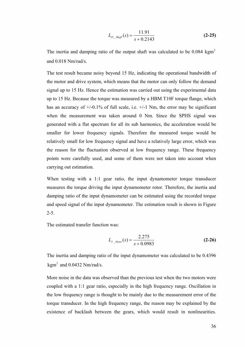
11.91LO _ Shaft (s) (2-25)

s 0.2143

The inertia and damping ratio of the output shaft was calculated to be 0.084 kgm2

and 0.018 Nm/rad/s.

The test result became noisy beyond 15 Hz, indicating the operational bandwidth of

the motor and drive system, which means that the motor can only follow the demand

signal up to 15 Hz. Hence the estimation was carried out using the experimental data

up to 15 Hz. Because the torque was measured by a HBM T10F torque flange, which

has an accuracy of +/-0.1% of full scale, i.e. +/-1 Nm, the error may be significant

when the measurement was taken around 0 Nm. Since the SPHS signal was

generated with a flat spectrum for all its sub harmonics, the acceleration would be

smaller for lower frequency signals. Therefore the measured torque would be

relatively small for low frequency signal and have a relatively large error, which was

the reason for the fluctuation observed at low frequency range. These frequency

points were carefully used, and some of them were not taken into account when

carrying out estimation.

When testing with a 1:1 gear ratio, the input dynamometer torque transducer

measures the torque driving the input dynamometer rotor. Therefore, the inertia and

damping ratio of the input dynamometer can be estimated using the recorded torque

and speed signal of the input dynamometer. The estimation result is shown in Figure

2-5.

The estimated transfer function was:

2.275LI _ Dyno (s) (2-26)

s 0.0983

The inertia and damping ratio of the input dynamometer was calculated to be 0.4396

kgm2 and 0.0432 Nm/rad/s.

More noise in the data was observed than the previous test when the two motors were

coupled with a 1:1 gear ratio, especially in the high frequency range. Oscillation in

the low frequency range is thought to be mainly due to the measurement error of the

torque transducer. In the high frequency range, the reason may be explained by the

existence of backlash between the gears, which would result in nonlinearities.

36

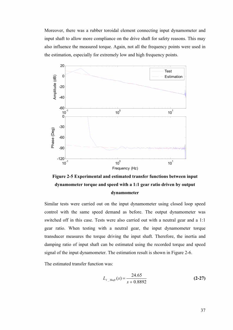
Moreover, there was a rubber toroidal element connecting input dynamometer and

input shaft to allow more compliance on the drive shaft for safety reasons. This may

also influence the measured torque. Again, not all the frequency points were used in

the estimation, especially for extremely low and high frequency points.

-1 0 110 10 10

-1 0 110 10 10

Frequency (Hz)

Figure 2-5 Experimental and estimated transfer functions between input

dynamometer torque and speed with a 1:1 gear ratio driven by output

dynamometer

Similar tests were carried out on the input dynamometer using closed loop speed

control with the same speed demand as before. The output dynamometer was

switched off in this case. Tests were also carried out with a neutral gear and a 1:1

gear ratio. When testing with a neutral gear, the input dynamometer torque

transducer measures the torque driving the input shaft. Therefore, the inertia and

damping ratio of input shaft can be estimated using the recorded torque and speed

signal of the input dynamometer. The estimation result is shown in Figure 2-6.

The estimated transfer function was:

24.65LI _ Shaft (s) (2-27)

s 0.8892

-60

-40

-20

0

20

Am

plitu

de (

dB)

Test

Estimation

-120

-90

-60

-30

0

Pha

se (

Deg

)

37

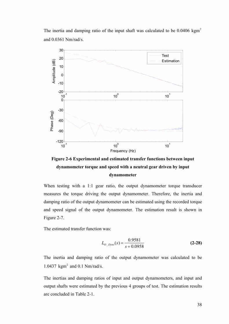
The inertia and damping ratio of the input shaft was calculated to be 0.0406 kgm2

and 0.0361 Nm/rad/s.

-1 0 110 10 10

-20

-10

0

10

20

30 A

mpl

itude

(dB

) Test

Estimation

10-1

100

101

-120

-90

-60

-30

0

Pha

se (

Deg

)

Frequency (Hz)

Figure 2-6 Experimental and estimated transfer functions between input

dynamometer torque and speed with a neutral gear driven by input

dynamometer

When testing with a 1:1 gear ratio, the output dynamometer torque transducer

measures the torque driving the output dynamometer. Therefore, the inertia and

damping ratio of the output dynamometer can be estimated using the recorded torque

and speed signal of the output dynamometer. The estimation result is shown in

Figure 2-7.

The estimated transfer function was:

0.9581LO _ Dyno (s) (2-28)

s 0.0958

The inertia and damping ratio of the output dynamometer was calculated to be

1.0437 kgm2 and 0.1 Nm/rad/s.

The inertias and damping ratios of input and output dynamometers, and input and

output shafts were estimated by the previous 4 groups of test. The estimation results

are concluded in Table 2-1.

38

-60

-40

-20

0

20

Am

plitu

de (

dB)

Test

Estimation

-1 0 110 10 10

10-1

100

101

-120

-90

-60

-30

0

Pha

se (

Deg

)

Frequency (Hz)

Figure 2-7 Experimental and estimated transfer functions between output

dynamometer torque and speed with a 1:1 gear ratio driven by input

dynamometer

Table 2-1 Estimation of system inertias and damping ratios

I/I/PP DDyynono I/PI/P ShaShafftt O/P ShO/P Shafaftt O/P DO/P Dyynono

IInernertitiaa

EEsstitimmaatitionon 00..44396396 00..04040606 0.0.008844 11..04304377

MaMannufaufactctururee 0.40.433 N/N/AA N/AN/A 0.0.99

TotTotaall 00..56564242

EEsstitimmaatitionon 00..00432432 00..03036161 0.0.001188 0.0.11

DaDampmpingingTotTotaall 00..09097373

Furthermore, when testing on the output dynamometer with a 1:1 gear ratio, the

output dynamometer torque transducer was measuring the torque driving the input

and output shafts and input dynamometer. The total inertia and damping ratio of

these three parts can be estimated using the recorded torque and speed signals of

output dynamometer to verify the previous results. The estimation results for total

inertia and damping ratio are shown in Figure 2-8.

39

-60

-40

-20

0

20

Am

plitu

de (

dB)

Test

Estimation

-1 0 110 10 10

10-1

100

101

-120

-60

0

60

120

180

Pha

se (

Deg

)

Frequency (Hz)

Figure 2-8 Experimental and estimated transfer functions between output

dynamometer torque and speed with a 1:1 gear ratio driven by output

dynamometer

Due to the backlash between the gears, the test result showed non-linear relationship

between measured torque and speed at high frequencies. The estimation was carried

out with a frequency range from 1 Hz to 3 Hz. It may represent the real system up to

6 Hz without obvious deviation from the test result. The estimated transfer function

was:

1.711LI _ D&Shs (s) (2-29)

s 0.2076

The inertia and damping ratio of the input dynamometer and the whole shaft were

calculated to be 0.5845 kgm2 and 0.1213 Nm/rad/s. The values calculated from

previous estimation were 0.5642 kgm2 and 0.0973 Nm/rad/s. The values estimated

for inertias are closer than the values estimated for damping ratios. From the

estimation results, the values of the damping ratios were very small compared to the

inertias, which will cause the cutoff frequency to be very low, e.g. 0.033 Hz in

Equation (2-29), and the lack of data to estimate the damping ratios. Moreover,

because the estimation of damping ratios relies on low frequency points, which are

affected by measurement errors, the damping estimation results were not as accurate

40

as the inertias. Hence, the dynamics of the system load are mainly determined by the

inertias of the system, especially in middle and high frequency range. Since the

damping ratios are very small, the damping effect can actually be neglected.

Although the experimental results shown in Figures 2-5 and 2-8 were obtained from

the same test on the output dynamometer speed control with a 1:1 gear ratio, the

backlash effects are major in the latter case. The result shown in Figure 2-5 was

obtained from the input dynamometer torque and speed signals, while the result

shown in Figure 2-8 was obtained from the output dynamometer torque and speed

signals. The load on the input dynamometer is the input dynamometer rotor, whereas

the load on the output dynamometer is the combination of the input and output shafts,

gear box, and the input dynamometer rotor. Therefore, the nonlinearity due to the

backlash in the gear box has more effects on the results in Figure 2-8. The effect is

significant above 10 Hz and would affect the performance of the feedforward

controller as will be discussed later.

2.2.2 Estimation of Motor and Drive System

The next component to be estimated in the block diagram shown in Figure 2-2 is the

motor and drive system. The motor and drive system takes a digital percentage

control signal as input, converts it into analogue voltage signal in the drive system,

and generates equivalent motor torque. There will be some dynamics between the

percentage control signal and motor torque, which can be identified from the

percentage and torque signals recorded in the test.

As mentioned above, the measured torque is the combined torque on the shaft. It is

different from the torque generated by the motor. For a single motor without any

external torque, the measured torque is the torque which is used to drive the

connected shaft. When the inertia or damping of the shaft changes, the measured

torque will change, even with the same control signal. Figure 2-9 shows the

frequency responses between measured torque and percentage control signal of

output dynamometer when running the motor with and without the output shaft

attached.

41

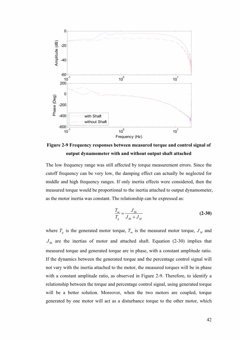
-60

-40

-20

0

Am

plitu

de (

dB)

-1 0 110 10 10

10-1

100

101

-600

-400

-200

0

200

Pha

se (

Deg

)

with Shaft

without Shaft

Frequency (Hz)

Figure 2-9 Frequency responses between measured torque and control signal of

output dynamometer with and without output shaft attached

The low frequency range was still affected by torque measurement errors. Since the

cutoff frequency can be very low, the damping effect can actually be neglected for

middle and high frequency ranges. If only inertia effects were considered, then the

measured torque would be proportional to the inertia attached to output dynamometer,

as the motor inertia was constant. The relationship can be expressed as:

Tm JSh (2-30)

Tg JSh JM

where Tg is the generated motor torque, Tm is the measured motor torque, J M and

JSh are the inertias of motor and attached shaft. Equation (2-30) implies that

measured torque and generated torque are in phase, with a constant amplitude ratio.

If the dynamics between the generated torque and the percentage control signal will

not vary with the inertia attached to the motor, the measured torques will be in phase

with a constant amplitude ratio, as observed in Figure 2-9. Therefore, to identify a

relationship between the torque and percentage control signal, using generated torque

will be a better solution. Moreover, when the two motors are coupled, torque

generated by one motor will act as a disturbance torque to the other motor, which

42

will also have effects on the measured motor torque, but not on the generated motor

torque.

Therefore, the model for motor and drive system was identified through a transfer

function between generated motor toque and percentage control signal, rather than

the measured torque. The generated motor torque can be calculated from the

measured motor torque and motor speed as follows:

Tg Tm J M M BM M (2-31)

where Tg is the generated motor torque, Tm is the measured motor torque, J M and

BM are the inertia and damping ratio of the motor, and M and M are the speed

and acceleration of the motor. J M and BM were identified in previous section. Tm

and M were recorded. M was calculated from M , by fitting a second order

polynomial to three speed samples and calculating derivatives at each sample point.

Since every speed sample was fitted a curve three times at the first, middle and last

point, the acceleration was also calculated three times for each sampling instance.

M used in Equation (2-31) was an average of these three values. The measured

relationship between generated motor torque and percentage control signal for output

dynamometer is shown in Figure 2-10, where there is no significant difference

between the results with and without the output shaft attached.

The test result shown in Figure 2-10 further established that the relationship between

generated motor torque and percentage control signal will not vary with the load

inertia. Therefore, the dynamics of the motor and drive system is better to be

interpreted using the generated motor torque instead of the measured motor torque.

Referring back to the control diagram in Figure 2-2, the torque would be the torque

generated by the motor and the load would be the external load plus the motor rotor

inertia.

43

-40

-20

0

20

40

Am

plitu

de (

dB)

-1 0 110 10 10

10-1

100

101

-400

-300

-200

-100

0

100

Pha

se (

Deg

)

With Shaft

Without Shaft

Frequency (Hz)

Figure 2-10 Frequency responses between generated torque and control signal

of output dynamometer with and without output shaft attached

The test results become noisy beyond 15 Hz, as observed from the previous test

results, which indicates the operation bandwidth of the motor. The smooth response

indicates linear characteristics of the motor. Since the frequency range of up to 15 Hz

was sufficient for testing CVTs, the estimation of motor and drive system model was

carried out within the smooth range between 1 Hz and 15 Hz using averaged values

from 5 tests. The estimated transfer function between generated torque and

percentage control signals for output dynamometer is as follows:

1.243s3 121.7s 2 2.468e4s 6.592e5GO _ Dyno (s)

3 2 (2-32)

s 97.29s 5660s 7.184e4

The frequency response of the estimated transfer function is shown in Figure 2-11,

compared with the averaged test results.

44

-40

-20

0

20

40

Am

plitu

de (

dB)

-1 0 110 10 10

10-1

100

101

-300

-200

-100

0

100

Pha

se (

Deg

)

Test

Estimation

Frequency (Hz)

Figure 2-11 Experimental and estimated transfer functions between generated

torque and control signal of output dynamometer

A similar identification procedure was carried out for the input dynamometer, also

within the frequency range of 1 Hz to 15 Hz. The estimated transfer function

between generated motor torque and percentage control signals was found to be:

0.7651s3 66.06s2 1.478e4s 5.141e5GI _ Dyno (s)

3 2 (2-33)

s 98.34s 6134s 9.429e4

The frequency responses of the estimated transfer function and averaged test results

are shown in Figure 2-12.

The transfer functions have been estimated for the motor and drive system for both

input and output dynamometers at a certain motor speed. The linear regions i.e.

different motor torques and speeds where the estimated transfer functions can

represent the motor behaviour need to be further established.

45

-30

-20

-10

0

10

20

Am

plitu

de (

dB)

-1 0 110 10 10

10-1

100

101

-250

-200

-150

-100

-50

0

Pha

se (

Deg

)

Test

Estimation

Frequency (Hz)

Figure 2-12 Experimental and estimated transfer functions between generated

torque and control signal of input dynamometer

Further tests were carried out with different levels of speed demands, each demand

consisting of a DC speed signal and an SPHS speed signal with an amplitude scaled

to 5% of the DC speed. For the output dynamometer, the steady state speed was

increased from 250 rev/min to 1500 rev/min, by 250 rev/min intervals. The torque

generated by the motor was increased relatively due to the larger acceleration of the

motor. The frequency response between generated torque and percentage control was

obtained by Fourier Transform as in previous tests, and are shown in Figure 2-13

with three different speeds, where the frequency responses were very similar to each

other. It can be concluded that the characteristics of output dynamometer and its

drive system is linear. The generated motor torque depended only on the percentage

control signal, but not on the motor torque or speed. The behaviour may be due to the

control strategy that exists in the drive system.

The dynamic response of the motor and drive system was also examined for the input

dynamometer in a similar way. Considering its application of emulating an IC engine,

the steady state speed demand for the input dynamometer was increased from 500

rev/min to 4000 rev/min in 500 rev/min interval, plus an SPHS speed signal with

46

scaled amplitude of 5% of the steady state speed. The results are shown in Figure

2-14 with three different steady state speeds.

-40

-20

0

20

40 A

mpl

itude

(dB

)

-1 0 110 10 10

-600

-400

-200

0

200

Pha

se (

Deg

)

500 rpm

1000 rpm 1500 rpm

-1 0 110 10 10

Frequency (Hz)

Figure 2-13 Frequency responses between generated torque and control signal

of output dynamometer with different speeds

-40

-20

0

20

40

Am

plitu

de (

dB)

-1 0 110 10 10

-400

-200

0

200

Pha

se (

Deg

)

1000 rpm

2000 rpm 3000 rpm

-1 0 110 10 10

Frequency (Hz)

Figure 2-14 Frequency responses between generated torque and control signal

of input dynamometer with different speeds

47

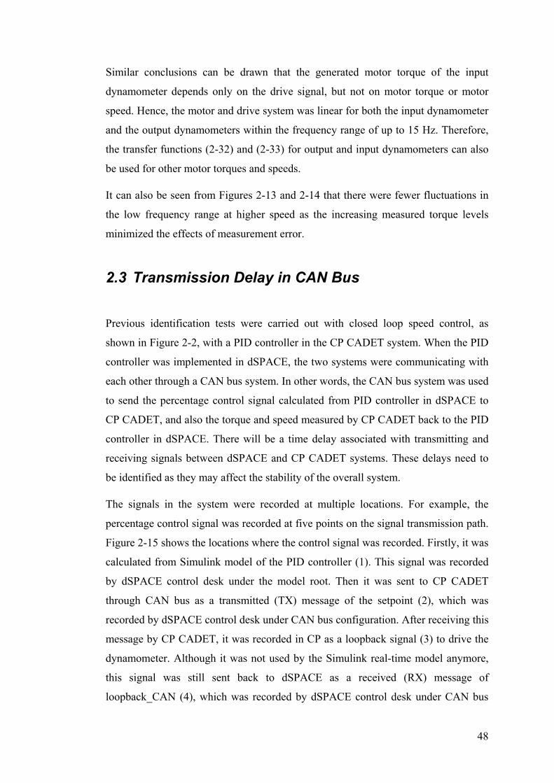
Similar conclusions can be drawn that the generated motor torque of the input

dynamometer depends only on the drive signal, but not on motor torque or motor

speed. Hence, the motor and drive system was linear for both the input dynamometer

and the output dynamometers within the frequency range of up to 15 Hz. Therefore,

the transfer functions (2-32) and (2-33) for output and input dynamometers can also

be used for other motor torques and speeds.

It can also be seen from Figures 2-13 and 2-14 that there were fewer fluctuations in

the low frequency range at higher speed as the increasing measured torque levels

minimized the effects of measurement error.

2.3 Transmission Delay in CAN Bus

Previous identification tests were carried out with closed loop speed control, as

shown in Figure 2-2, with a PID controller in the CP CADET system. When the PID

controller was implemented in dSPACE, the two systems were communicating with

each other through a CAN bus system. In other words, the CAN bus system was used

to send the percentage control signal calculated from PID controller in dSPACE to

CP CADET, and also the torque and speed measured by CP CADET back to the PID

controller in dSPACE. There will be a time delay associated with transmitting and

receiving signals between dSPACE and CP CADET systems. These delays need to

be identified as they may affect the stability of the overall system.

The signals in the system were recorded at multiple locations. For example, the

percentage control signal was recorded at five points on the signal transmission path.

Figure 2-15 shows the locations where the control signal was recorded. Firstly, it was

calculated from Simulink model of the PID controller (1). This signal was recorded

by dSPACE control desk under the model root. Then it was sent to CP CADET

through CAN bus as a transmitted (TX) message of the setpoint (2), which was

recorded by dSPACE control desk under CAN bus configuration. After receiving this

message by CP CADET, it was recorded in CP as a loopback signal (3) to drive the

dynamometer. Although it was not used by the Simulink real-time model anymore,

this signal was still sent back to dSPACE as a received (RX) message of

loopback_CAN (4), which was recorded by dSPACE control desk under CAN bus

48

configuration. After receiving this signal by the real-time model, this signal was

recorded again as loopback_Sim (5) by dSPACE control desk under the model root.

Control Signal Facilities Locations TX Message RX Message

Sim

CAN

CP

Percentage control signal

Loopback_CP

Setpoint Loopback_CAN

Loopback_Sim dSPACE

dSPACE

CADET

(1)

(2)

(3)

(4)

(5)

Figure 2-15 Recording locations for the percentage control signal

By comparing the same signal recorded from different locations in the system, the

delay in transmitting and receiving messages can be identified. Figure 2-16 shows

the control signal recorded by dSPACE control desk in Simulink model and CAN

bus configuration, which were synchronized by dSPACE. The control signal

recorded by CP CADET is not shown, because it was not synchronized with

dSPACE.

9.7 9.75 9.8 9.85 9.9 -10

-5

0

5

10

Con

trol

Sig

nal (

%)

Percentage (1)

Setpoint (2) Loopback-CAN (4)

Loopback-Sim (5)

Time (s)

Figure 2-16 Percentage control signal recorded in different locations

Together with Figure 2-15, it can be observed that there are two samples delay from

percentage signal (1) to setpoint signal (2), and no delay from loopback_CAN (4) to

loopback_Sim (5). From setpoint (2) to loopback_CAN (4), there was one sample

49

delay. This one sample delay could exist either between setpoint (2) and

loopback_CP (3), or between loopback_CP (3) and loopback_CAN (4). To examine

this, different sampling frequencies were used for the CAN bus and CP control

system. It was observed that the length of this delay varied with the CP control

frequency, but not with the CAN bus sampling frequency. It was always one sample

delay of CP control rate, which meant the delay existed between loopback_CP (3)

and loopback_CAN (4). Different sampling frequencies were also applied to the

Simulink model and the CAN bus. It was observed that the two samples delay

between percentage (1) and setpoint (2) was depended on the Simulink model

sampling rate. The delays on signal transmitting path in the system were concluded

as in Figure 2-17.

Facilities Locations Data

Sim

CAN

CP

dSPACE

dSPACE

CADET

2 model sampling delay

1 CP sampling delay No delay

No delay

TX Message RX Message

Figure 2-17 Delays on signal transmitting path

Normally, the sampling rate on the CAN bus system is slower than the simulation

sampling rate by an integer divider. Delay in the TX message was dependent on the

simulation sampling rate, while delay in the RX message was dependent on the

control frequency in the CP CADET system. In the tests with the CAN bus, the

percentage control signal calculated from the real-time model was sent to CP

CADET as a TX message to drive the dynamometer, the delay can be reduced by

increasing sampling rate in Simulink model to be as small as required. Measured

torque and speed signals were sent back to the real-time Simulink model as RX

message to calculate next control signal sample. The delay was restricted to be at

least 6.25 ms, as the fastest control rate available on the CP CADET system is 160

Hz.

50

2.4 Model for Speed Control with CAN Bus Delay

When the CAN bus is implemented in the system to forward messages, the effects of

the delays identified in previous section have to be considered. This was first

examined for the output dynamometer speed control system. A Simulink model was

constructed based on the identified models for the system components, and the

effects of CAN bus delay on the system was investigated in simulation in order to

retune the PID controller parameters. Then a transfer function for the whole closed

loop system was derived to design the feedforward controller in the next chapter.

Alternatively, the transfer function can be estimated directly from the test results

between the speed demand signal and the measured speed signal. Both methods are

described here and compared with test results.

2.4.1 Simulink Model

Based on the speed control diagram shown in Figure 2-2, a CAN bus system can be

incorporated into the model. The PID controller is placed in dSPACE instead of in

the CP CADET system. The output of PID controller, the percentage control signal,

is sent to CP console through the CAN bus. The measured speed is then sent back to

dSPACE through CAN bus. The block diagram is shown in Figure 2-18.

PID Controller

PIDController

Motor & Drive System

Load+

-

Speed SP Speed Response

dSPACE

2z

Percentage Torque

1z

Delayed Response

CAN

Figure 2-18 Speed control block diagram with CAN bus delay

After including the delays in the model, if the same PID parameters as in the CP

CADET system are used, the simulation results in Figure 2-19 show oscillations in

the speed response. The speed demand consisted of a DC speed of 1000 rev/min plus

an SPHS signal with frequency up to 15 Hz and an amplitude of 40 rev/min.

51

0 2 4 6 8 10 850

900

950

1000

1050

1100

1150

Spe

ed (

rev/

min

)

Demand

Simulated Response

Time (s)

Figure 2-19 Simulated speed response with CAN bus and original PID

parameters

The performance can be improved by retuning the PID parameters. This was first

performed in simulation. Improved PID parameters were found to be 0.13 for

proportional gain, 0.25 for integral gain, and 0 for derivative gain, which yields a

new transfer function for the PID controller as follows:

0.13s 0.25GPID (s) (2-34)

s

Simulations were run with these new PID parameters, with the same speed demand

as before. The test results are shown in Figure 2-20.

0 2 4 6 8 10 950

1000

1050

Spe

ed (

rev/

min

)

Demand

Simulated Response

Time (s)

Figure 2-20 Simulated speed response with CAN bus and new PID parameters

52

Actual tests were carried out with the same speed demand to validate the Simulink

model. The simulation results and test results are compared in Figure 2-21.

Magnified views are shown in Figure 2-22.

950

1000

1050

Spe

ed (

rev/

min

)

Simulated

Test

0 2 4 6 8 10 Time (s)

Figure 2-21 Comparison of simulation and test results of output dynamometer

speed control with new PID parameters

1050 1010 1002

1001 1025 1005

Spe

ed (

rev/

min

)

1000

1000 1000

999

975 995 998

950 990 997 1 1.5 2 5 5.2 5.4 9 9.1 9.2

Time (s)

Figure 2-22 Magnified view of Figure 2-21

It can be seen that the simulation results offered a good fit to the test results, but

there are some fluctuations for high frequency components, due to the small

amplitude, hence high noise to signal ratio, of the signal. Comparison was also

performed in the frequency domain in Figure 2-23. The frequency response was

calculated by taking the Fourier Transform of the speed demand and speed response

in both simulation and test results.

53

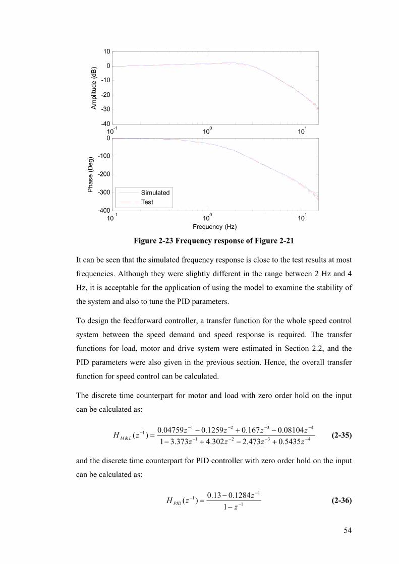
-40

-30

-20

-10

0

10

Am

plitu

de (

dB)

-1 0 110 10 10

10-1

100

101

-400

-300

-200

-100

0

Pha

se (

Deg

)

Simulated

Test

Frequency (Hz)

Figure 2-23 Frequency response of Figure 2-21

It can be seen that the simulated frequency response is close to the test results at most

frequencies. Although they were slightly different in the range between 2 Hz and 4

Hz, it is acceptable for the application of using the model to examine the stability of

the system and also to tune the PID parameters.

To design the feedforward controller, a transfer function for the whole speed control

system between the speed demand and speed response is required. The transfer

functions for load, motor and drive system were estimated in Section 2.2, and the

PID parameters were also given in the previous section. Hence, the overall transfer

function for speed control can be calculated.

The discrete time counterpart for motor and load with zero order hold on the input

can be calculated as:

H (z 1 ) 0.04759z 1 0.1259z 2 0.167z 3 0.08104z 4

(2-35)M &L 1 2 3 41 3.373z 4.302z 2.473z 0.5435z

and the discrete time counterpart for PID controller with zero order hold on the input

can be calculated as:

1 0.13 0.1284z 1

H PID (z ) 1 z 1

(2-36)

54

According to the control diagram shown in Figure 2-18, including the delays in the

system, the closed loop discrete time transfer function between the speed demand

and speed response can be obtained as follows:

0.006186z 4 0.02248z 5 0.03788z 6

H Close (z 1 ) 0.03199z 7 0.01041z 8

(2-37)1 4.373z 1 7.675z 2 6.775z 3 3.023z 4

0.5659z 5 0.03788z 6 0.03199z 7 0.01041z 8

The frequency response of the calculated closed loop transfer function is shown in

Figure 2-24, compared with the experimental transfer function between derived and

demanded speed signals.

-1 0 110 10 10

-40

-30

-20

-10

0

10

Am

plitu

de (

dB)

10-1

100

101

-400

-300

-200

-100

0

Pha

se (

Deg

)

Test

Calculated Transfer Function

Frequency (Hz)

Figure 2-24 Experimental and calculated transfer function of output

dynamometer speed control

The overall transfer function in Equation (2-37) was calculated from separate transfer

functions, which were estimated within the frequency range of 1 Hz to 15 Hz, and

therefore it represents the system within this frequency range.

55

2.4.2 Estimated Transfer Function

The overall transfer function could also be estimated directly by taking speed

demand as input signal and speed response as output signal. The estimation was

carried out within the frequency range of 1 Hz and 15 Hz. Different orders were

specified for numerator and denominator of the estimated transfer function. The

statistical analysis results showed that a third order for numerator and fourth order

for denominator provided the best fit. The estimation result is as follows:

1.096s3 47.86s 2 2043s 1.336e6GClose (s) (2-38)

s 4 77.91s3 5598s 2 9.494e4s 1.336e6

The equivalent discrete time transfer function with 160 Hz sampling frequency and

zero order hold on the input is:

(z 1 ) 0.004442z 1 0.0142z 2 0.01713z 3 0.005788z 4

(2-39)H Close 1 3.434z 1 4.503z 2 2.682z 3 0.6145z 4

The frequency response of estimated transfer function is shown in Figure 2-25, and

compared with test results.

-1 0 110 10 10

-1 0 110 10 10

Frequency (Hz)

Figure 2-25 Experimental and estimated transfer functions of output

dynamometer speed control

-40

-30

-20

-10

0

10

Am

plitu

de (

dB)

-400

-300

-200

-100

0

Pha

se (

Deg

)

Test

Estimated Transfer Function

56

The estimated transfer function offered a better fit than the calculated transfer

function in the middle frequency range, but a slightly worse fit in the low frequency

range. Both calculated and estimated transfer functions can be considered as a good

fit to the test results.

Frequency responses of the calculated transfer function and estimated transfer

function are compared in Figure 2-26. The frequency range to be shown was

extended to 50 Hz.

-1 0 110 10 10

-60

-40

-20

0

20

Am

plitu

de (

dB)

10-1

100

101

-800

-600

-400

-200

0

Pha

se (

Deg

)

Calculated Transfer Function

Estimated Transfer Function

Frequency (Hz)

Figure 2-26 Calculated and estimated transfer functions of output dynamometer

speed control

It can be seen that the calculated and estimated transfer functions possess different

characteristics, but within the frequency range, where the estimation was carried out,

they produced similar results.

Comparing the calculated transfer function in Equation (2-37) and estimated transfer

function in Equation (2-39), the orders of the numerator and denominator are

different. In Equation (2-37) the relative order, i.e. order of the denominator minus

numerator, is four, while in Equation (2-39) the relative order is only one. When the

overall transfer function is estimated, the relative order is specified to achieve a good

fit for only the interested frequency range, rather than the whole frequency range.

Moreover, in Equation (2-38), all the poles and zeros have break efficiencies within

57

20 Hz. They are considered to be significant to the system within the interested

frequency range so that the estimated transfer function can not be simplified anymore.

This characteristic is very useful and will be utilized in the design of a feedforward

controller. It is beneficial to have a smaller relative order when inverting the transfer

function, because smaller relative order means that less future sampling values are

needed to implement the controller. This will be discussed in detail in the next

chapter.

58

Chapter 3

Feedforward Tracking Controller

In the previous chapter, a methodology was presented to identify the dynamics of a

linearized system in the desired frequency range, leading to a continuous time

transfer function, and its counterpart in discrete time was obtained by placing a zero

order hold on the input signal. The discrete time transfer function is now used to

create an inverse system to be used as a feedforward controller.

The concepts of minimum and non-minimum phase system are introduced first.

Direct inverse for minimum phase systems is stable and straightforward. For non-

minimum phase systems, the technique of developing a digital preview filter (DPF)

is employed here to approximate the inverse of unstable zeros using Lagrange

method as part of the feedforward controller. To apply DPFs, future information of

the input trajectory was required. Normally, the future values can be predicted in

some way, but the prediction can never be perfect, and will certainly affect the

control performance. In this chapter, DPFs will be designed for the output

dynamometer speed control and input dynamometer torque control in a novel way, so

that no future information of input trajectories is required, which allows a non-causal

controller to be causal.

3.1 Digital Preview Filter

On an approximate inversion of a non-minimum system, the zero phase error

tracking control (ZPETC) has drawn interest among researchers, because zero phase

shift is obtain at all frequencies, with a small gain error at low frequencies. Based on

ZPETC, a precision tracking control scheme was proposed in [51] to further improve

gain characteristics at higher frequencies. The optimal design was also obtained by

Lagrange method.

59

One of the merits of this scheme was that a weighting function can be incorporated

into the penalty function. This will ensure the gain error is better compensated in the

desired frequency range. The parameterization of the digital preview filter was

presented in an explicit form. Given a discrete time transfer function, the filter could

easily be parameterized to minimize the penalty function with a fixed number of

preview steps. The preview steps can be chosen arbitrarily. Generally, a greater

number of available preview steps renders better tracking performance.

3.1.1 Design of DPF

The feedforward control scheme as shown in Figure 1-7, Q(z1) is the feedforward

controller transfer function, and H (z1) is the original system transfer function,

which can be either closed or open-loop. When the system is a non-minimum phase

system, the transfer function can normally be separated into two parts:

H (z1) Ha (z1)Hu (z1) (3-1)

in which H u (z 1 ) includes all the unstable zeros.

P

H u (z 1 ) (1 zi z 1 ) (3-2) i1

H a (z 1 ) can be directly inverted to be H a 1 (z 1 ) as part of feedforward controller. A

digital preview filter DPF (z 1 ) can be designed to approximate H u1 (z 1 ) as another

part of feedforward controller. Hence, the feedforward controller can be expressed as:

Q(z 1 ) H a1 (z 1 )H u

1 (z 1 ) H a 1 (z 1 )DPF (z 1 ) (3-3)

The ratio R(z 1 ) is defined as follows to measure the tracking performance:

P

R(z 1 ) DPF(z 1 ) (1 zi z 1 ) (3-4) i1

To achieve perfect tracking, the ratio function R(z 1 ) should have a unity gain and

zero phase shift within the desired frequency range. To achieve this objective, the

digital preview filter DPF(z 1 ) is divided into two parts as follows:

60

DPF (z 1 ) DPFA (z 1 )DPF (z 1 ) (3-5)

where DPF (z 1 ) is to make the digital preview filter have the same phase as that of

H u 1 (z 1 ) , and DPFA (z 1 ) is to make the gain of the digital preview filter to be as

close to that of H u1 (z 1 ) as possible.

The design of DPF (z 1 ) was initially presented in [47] as ZPETC controller.

P (1 z z)DPF (z 1 ) i (3-6)

(1 z )(1 z )i1 i i

where zi is the complex conjugate of the unstable zero zi . The denominator in

Equation (3-6) ensures a unity DC gain. Substituting Equations (3-5) and (3-6) into

Equation (3-4), the ratio function R(z 1 ) becomes:

P 1

R(z 1 ) DPFA (z 1 ) (1 zi z)(1 zi z )

(3-7) i1 (1 zi )(1 zi )

If, among P unstable zeros, there are P1 real unstable zeros, and P2 pairs of the

complex unstable zeros, Equation (3-7) can be rewritten as:

1 1 0 1 1 0 1 1 2 1 2R(z ) DPF (z ) P1 (z z )

P2 (z z ) (z z ) A k k j j j k 1 j1

P

DPFA (z 1 ) i (z z 1 ) i

i0

(3-8)

where

1 z 2 zk

0 k k 1 k

(1 zk )2 (1 zk )

2

j 0

1 2(2cos2 j 1)rj 2

2

2

rj 4

1 j

2rj cos j (1 r 2

j 2 )

2 j

2 rj

2

2 2(1 2rj cos j rj ) (1 2rj cos j rj ) (1 2rj cos j rj )

(3-9)

61

In which rj and j are the magnitude and argument of the complex unstable zeros.

It can be seen from Equation (3-8) that DPF (z 1 )H u (z 1 ) can be expressed as a

function of z z 1 and has zero phase shift. In fact, z z 1 is a minimal zero phase

filter and it is defined as the zero phase kernel in [51]. To make R(z 1 ) to have a

zero phase shift, DPFA (z 1 ) must also have zero phase shift. Therefore, it can be

also formulated as a function of the zero phase kernel as:

N P

DPFA (z 1 ) k (z z 1 ) k (3-10) k 0

where N is the required preview steps of the digital preview filter. Now the ratio

function can be expressed as:

R(z 1 )

P

i (z z 1 ) i

N

P

k (z z 1 ) k (3-11)

i0 k 0

3.1.2 Norm Optimization for DPF

The coefficients k can be determined by minimizing the following penalty function

J, formulated by L2 norm:

J

w( )R(e j ) 12 d (3-12)

0

with the constraint:

R(e j ) 1 (3-13) 0

where is the normalized frequency, Ts , is the frequency, Ts is the

sampling time, and w( ) is the weighting function, which can be chosen according

to particular applications and the available information. The constraint in Equation

(3-13) is to ensure that both the digital preview filter DPF (z 1 ) and the unstable

inverse model H u 1 (z 1 ) have the same DC gain. In order to obtain the L2 norm

optimal solution for the polynomial parameters, k , Lagrange method is employed

here. The Lagrange function ( ,) is defined as:

62

( ,)

w( )R(e j ) 12 d R(e j ) 1 (3-14)

00

where is the Lagrange multiplier. From (3-11), R(e j ) can be expressed as:

R(e j )

p

i (2cos )i

N

p

k (2cos )k

i0 k0 1

T 2cos

N p γ

1 2cos (2cos ) α

p (2cos ) (3-15)

1 2cos (2cos )N p

2cos (2cos )2 (2cos )N p1 γT α

p p1 N (2cos ) (2cos ) (2cos )

γT Aα

where

Tγ 0 1 p Tα 0 1 N p (3-16)

1 2cos (2cos )N p 2 N p1 2cos (2cos ) (2cos ) A (2cos ) p (2cos ) p1 (2cos )N

Therefore,

R(e j ) 12 R(e j )2

2R(e j ) 1(3-17)

αT AT γγT Aα 2γT Aα 1

and

0

R(e j ) 1 2 2N p

1

βT α (3-18)

0

N p

where

63

N β 1 2 2 p T (3-19)

By substituting Equations (3-17) and (3-18) into Equation (3-14), it is obtained that:

αT A1α 2γT A2α w( )d (βT α 1) (3-20)

0

where

A1 w( )AT γγT Ad A2 w( )Ad (3-21)

0 0

Let

2A1α 2AT

2 γ β 0 (3-22)α

βT α 1 0 (3-23)

Multiplying both sides of Equation (3-22) by the matrix βT A1 1 :

2βT α 2βT A1 1AT

2 γ βT A1 1β 0 (3-24)

From Equation (3-23):

βT α 1 (3-25)

By substituting Equation (3-25) into Equation (3-24), the Lagrange multiplier can be

obtained as:

βT A1AT γ 1 2 1 T

21

(3-26)β A1 β

Again by substituting Equation (3-26) into Equation (3-22), optimal parameters of

DPFA (z 1 ) can be obtained as:

α A1 1

AT2 γ

1 βT

T

A1

1

1

AT 2 γ β

(3-27)

β A1 β

where the definition of the notations is given in Equations (3-16), (3-19) and (3-21).

It can be seen from Equations (3-6) and (3-10), that the DPF is non-causal. To

implement it, N future values are required, among which, P steps are required to

64

compensate the phases shift, and N-P steps are required to further compensate the

amplitude at the frequency range of interest. Additional preview steps may also be

required due to the relative order R of the transfer function when taking the inverse

of the stable part. Therefore the total number of preview steps required for the

feedforward controller is as follows:

D N R (3-28)

3.2 Causal Design of DPF

The digital preview filter described in the previous section solved two problems in

the design of feedforward controller: (a) improved the gain characteristics and (b)

provided an optimal solution. The problem of causality will be dealt with in this

section. Because the DPF is non-causal, N steps of future value of input trajectory are

needed to implement it. Otherwise, the tracking will be delayed by N steps.

Generally speaking, a larger N will render better tracking performance if the desired

trajectory is known prior. In the case that the desired trajectory is not known in

advance, a prediction method is needed for the feedforward controller. However, a

larger N will make the future values harder to predict. Several examples of predictor

can be found in literature, e.g. [58,69,70]. But there are no perfect prediction

technique, errors in the prediction may jeopardise control performance.

It is proposed in this section to make the application of DPF causal within a desired

frequency range by employing system identification techniques. Additional time

delays will be manually added after the measured response. The stability of the

closed loop system will be ensured by retuning the PID parameters after adding

manual delays. Then the feedforward controller will be designed according to this

delayed signal rather than the actual response signal. If the overall delay from the

delayed response to the actual response is made equal to the prediction length, then

the actual response will be tracking the demand without any preview action.

The following process was developed to eliminate the need to provide future values

of the reference signal in the design of feedforward controller:

65

(a) Guess the D value, i.e. the total number of preview steps required for the

feedforward controller.

(b) Add manual delays after actual response, equal to D minus the delay that

already exists in the CAN bus. Retune the feedback controller parameters for

closed loop system if necessary.

(c) Identify the transfer function of the new system with the added delay between

the demand signal and delayed response signal by seeking as low a relative

order R.

(d) Check if the selected number of preview steps D is appropriate by taking into

account of the relative order R and the number of unstable zeros P of the

estimated transfer function.

(d1) if (d) is satisfied, design the non-causal digital preview filter as

described in Section 3.1.

(d2) if (d) is not satisfied, select a different D, and repeat the process

There is one premise that after adding the manual delay, the total delay D from the

actual response to the delayed response must be much greater than the relative order

of estimated transfer function R.

Normally, after adding the manual delays, the relative order of the transfer function

between the demanded and delayed responses should be increased by D. The relative

order can be significantly reduced by seeking a lower R when identifying the delayed

system transfer function within a desired frequency range. So using the estimated

transfer function with a smaller relative order R for the feedforward controller design

can allocate more preview steps N for the inverse of the unstable zeros, among which,

P delays are used to compensate the phase, and N-P delays are used to further

compensate the amplitude. Generally speaking, better performance in compensating

amplitude error can be expected if more preview steps are available.

The selection of the D value is very flexible. Larger D may allow larger N (assuming

the same R) and larger N-P (assuming the same P) to compensate the amplitude error,

which will render a better compensation performance. But adding more delays to the

system will probably result in a higher relative order R in the estimated transfer

function to provide a good fit into test results. Even though the relative order can be

arbitrarily specified, adding more delays may cause the number of unstable zeros, P,

66

to increase. So, D-R-P may not increase as D increases, which will not help to

improve the performance of DPF. On the contrary, smaller D may result in smaller R

or P, which may provide better performance than larger D value. Therefore, it is hard

to say that larger or smaller D value is better. It needs to be evaluated for the specific

application.

Examples of the application of the proposed process in the design of the feedforward

controller for both closed loop and open-loop systems are given in the following

sections. Feedforward controllers are designed and implemented for the closed loop

speed control of the output dynamometer and the open-loop torque control of the

input dynamometer.

3.3 Causal Application of DPF to a Single Motor

The proposed causal design of digital preview filters is applied to a single motor in

this section. Feedforward controllers are designed for the output dynamometer speed

and the input dynamometer torque control.

3.3.1 Output Dynamometer Speed Tracking Control

The speed control diagram including sampling delay on the CAN bus is shown in

Figure 2-18, and the response to an SPHS demand signal with a frequency range up

to 15 Hz is shown in Figure 2-20. To carry out the process proposed in the previous

section, another 7 delays are added to the feedback loop in dSPACE as shown in

Figure 3-1.

PID Controller

Motor & Drive System

Load+

-

dSPACE

2z

Percentage Torque

1z7z

Manual Delay

CAN

Feedforward Controller

Feedforward Controller

dy r y

fy

Figure 3-1 Speed control block diagram with manual delay

67

900

950

1000

1050

1100

Spe

ed (

rev/

min

)

Demand

Delayed Response

The PID controller was retuned in simulation without the feedforward controller to

ensure the stability of the closed loop system. New PID parameters were selected as

0.15 for proportional control, 0.25 for integral control and 0.003 for derivative

control. Tests were carried out with a speed demand signal, r, consisting of a SPHS

signal superposed on a 1000 rev/min constant value. The delayed response of the

system, y f , is shown in Figure 3-2. The test result shown here is the average over

three tests.

0 2 4 6 8 10 Time (s)

Figure 3-2 Delayed system response of output dynamometer speed control with

7 manual delays

By using the FFT of the recorded signals, and setting the relative order to one, the

transfer function between the delayed speed response y f and speed demand r, was

estimated as follows:

4.979s5 761.8s 4 8.979e4s3 4.705e6s 2

9.175e7s 2.303e9GSpeed (s)

s 6 116s5 1.23e4s 4 6.978e5s3 1.628e7s 2 (3-29)

2.321e8s 2.303e9

This gives four unstable zeros. The frequency response of the estimated and

experimental transfer functions are shown in Figure 3-3. Because of the added delays,

the phase shift of the speed response was increased, especially at high frequencies.

The phase shift is approximately 550 degrees at 15 Hz.

In order to design the digital preview filter, a discrete time equivalent of the

estimated transfer function between delayed speed response y f and speed demand r

68

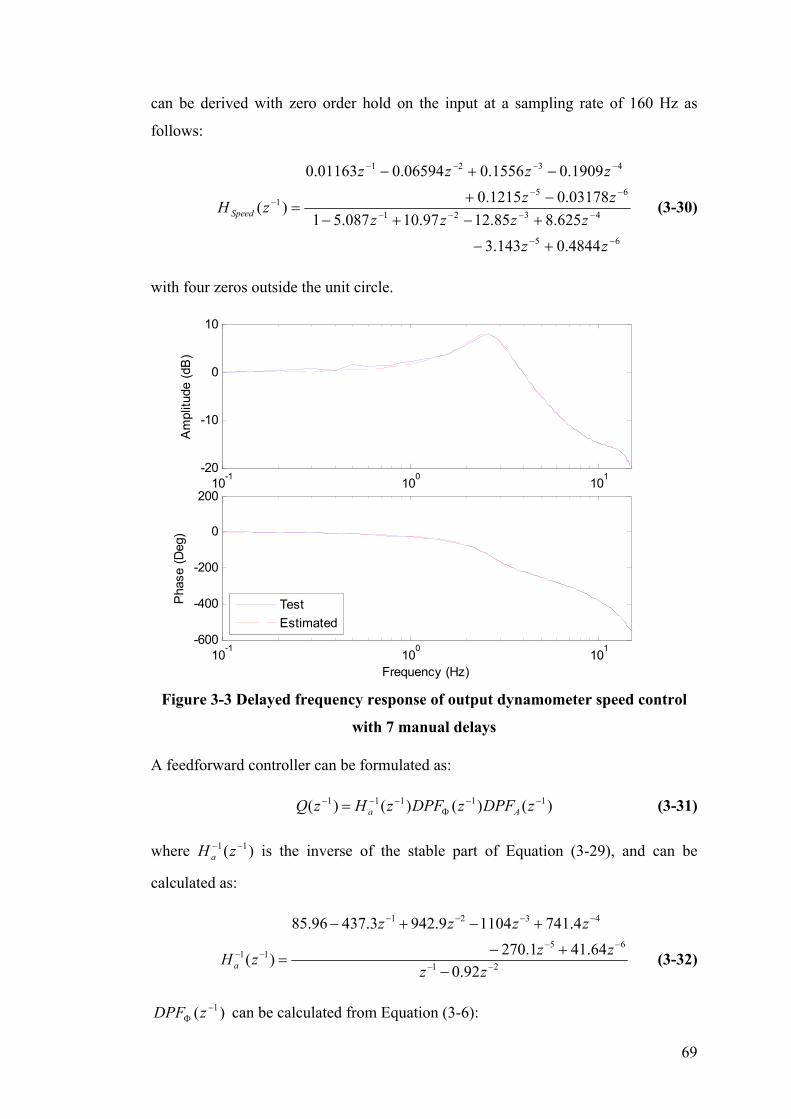
can be derived with zero order hold on the input at a sampling rate of 160 Hz as

follows:

0.01163z 1 0.06594z 2 0.1556z 3 0.1909z 4

1 0.1215z 5 0.03178z 6

H Speed (z ) 1 5.087z 1 10.97z 2 12.85z 3 8.625z 4

(3-30)

3.143z 5 0.4844z 6

with four zeros outside the unit circle.

-1 0 110 10 10

-1 0 110 10 10

Frequency (Hz)

Figure 3-3 Delayed frequency response of output dynamometer speed control

with 7 manual delays

A feedforward controller can be formulated as:

Q(z 1) H a1(z 1)DPF (z 1)DPFA (z 1) (3-31)

where H a 1(z1) is the inverse of the stable part of Equation (3-29), and can be

calculated as:

85.96 437.3z1 942.9z2 1104z3 741.4z4

1 1 270.1z5 41.64z6

Ha (z ) 1 2 (3-32)

z 0.92z

DPF (z 1 ) can be calculated from Equation (3-6):

-20

-10

0

10

Am

plitu

de (

dB)

-600

-400

-200

0

200

Pha

se (

Deg

)

Test

Estimated

69

DPF (z 1) 2.969 8.127z 1 9.007z 2 4.749z 3 z 4

(3-33)0.01015z 4

Then was obtained from Equations (3-8) and (3-9) to be:

103 [3.6252 7.7021 6.1548 2.1900 0.2926]T

Because the total delay D is 8 and the relative order of estimated transfer function R

is 1, the preview steps for digital preview filter N can be chosen to be D-R=7, and the

number of unstable zeros P=4. The weighting function w( ) was specified to be

uniform within the frequency range of up to 15 Hz, That is:

1 3

w( )

16 (3-34) 0

3 16

The penalty function J becomes:

J 16

3 R ( e j ) 1 2 d (3-35)

0

The matrices A1 and A2 are defined as:

3 3

A 16

AT γγT Ad A 16

Ad (3-36)1 0 2 0

Then the polynomial parameter vector for DPFA (z 1 ) can be calculated from

Equation (3-27) as:

19.2762 31.0421 15.9952 2.5216T

This gives the following digital preview filter to compensate for the amplitude using

Equation (3-10):

2.522 16z1 38.61z2 51.27z3 38.61z4

1 16z5 2.522z6

DPFA(z ) 3 (3-37)

z

One preview step is needed in Equation (3-32) because the relative order is one

(R=1). This leaves a total of 7 preview steps for the DPF design (N=7). Four preview

steps are needed in Equation (3-33) for the design of ZPETC, because the number of

70

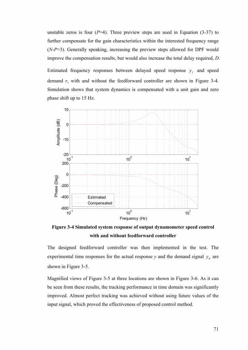
unstable zeros is four (P=4). Three preview steps are used in Equation (3-37) to

further compensate for the gain characteristics within the interested frequency range

(N-P=3). Generally speaking, increasing the preview steps allowed for DPF would

improve the compensation results, but would also increase the total delay required, D.

Estimated frequency responses between delayed speed response y f and speed

demand r, with and without the feedforward controller are shown in Figure 3-4.

Simulation shows that system dynamics is compensated with a unit gain and zero

phase shift up to 15 Hz.

-1 0 110 10 10

-20

-10

0

10

Am

plitu

de (

dB)

10-1

100

101

-600

-400

-200

0

200

Pha

se (

Deg

)

Estimated

Compensated

Frequency (Hz)

Figure 3-4 Simulated system response of output dynamometer speed control

with and without feedforward controller

The designed feedforward controller was then implemented in the test. The

experimental time responses for the actual response y and the demand signal yd are

shown in Figure 3-5.

Magnified views of Figure 3-5 at three locations are shown in Figure 3-6. As it can

be seen from these results, the tracking performance in time domain was significantly

improved. Almost perfect tracking was achieved without using future values of the

input signal, which proved the effectiveness of proposed control method.

71

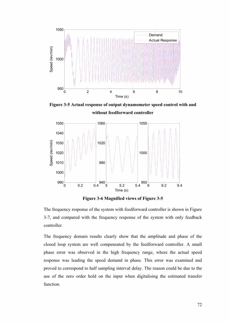
0 2 4 6 8 10 950

1000

1050

Spe

ed (

rev/

min

)

Demand

Actual Response

Time (s)

Figure 3-5 Actual response of output dynamometer speed control with and

without feedforward controller

0 0.2 0.4 990

1000

1010

1020

1030

1040

1050

Spe

ed (

rev/

min

)

5 5.2 5.4 940

980

1020

1060

9 9.2 9.4 950

1000

1050

Time (s)

Figure 3-6 Magnified views of Figure 3-5

The frequency response of the system with feedforward controller is shown in Figure

3-7, and compared with the frequency response of the system with only feedback

controller.

The frequency domain results clearly show that the amplitude and phase of the

closed loop system are well compensated by the feedforward controller. A small

phase error was observed in the high frequency range, where the actual speed

response was leading the speed demand in phase. This error was examined and

proved to correspond to half sampling interval delay. The reason could be due to the

use of the zero order hold on the input when digitalising the estimated transfer

function.

72

-20

-10

0

10

Am

plitu

de (

dB)

-1 0 110 10 10

10-1

100

101

-600

-400

-200

0

200

Pha

se (

Deg

)

Only Feedback Control

With Feedforward Control

Frequency (Hz)

Figure 3-7 Frequency response of Figure 3-5

As discussed in precious section, the selection of the D value is very flexible. Greater

D will not guarantee a better compensation performance. In the test, different

numbers of manual delays were added to the feedback loop, to offer different D

values. Transfer functions were estimated and feedforward controllers were designed

for each estimated transfer function. The information for the estimation and

feedforward controller design is summarised in Table 3-1. The frequency responses

of the estimated transfer functions are shown in Figure 3-8, and the simulated

frequency responses of the compensated systems are shown in Figure 3-9. It can be

seen that zero phase shift was achieved in all the three cases. The amplitude

compensation results are definitely improved by increasing the total number of the

delays from 6 to 8, but not so obviously from 8 to 10. Hence, D equal to 8 was

chosen and the designed feedforward controller was implemented in the test.

Table 3-1 Estimation and feedforward controller design with different D values

ToTottaall DDeellaayyss((DD))

ReRellaativtivee OrOrderder((RR))

PrPreveviieeww SStteeppss forfor DPFDPF ((NN))

((PP)) ((N-PN-P))

66 0 (40 (4thth/4/4thth)) 44 22

88 1 (51 (5thth/6/6thth)) 44 33

1010 1 (51 (5thth/6/6thth)) 44 55

73

-30

-20

-10

0

10

20

Am

plitu

de (

dB)

-1 0 110 10 10

-800

-600

-400

-200

0

Pha

se (

Deg

)

D=6

D=8 D=10

-1 0 110 10 10

Frequency (Hz)

Figure 3-8 Frequency responses of the estimated transfer functions with

different D values

-2

-1

0

1

2

Am

plitu

de (

dB)

-1 0 110 10 10

-1

-0.5

0

0.5

1

Pha

se (

Deg

)

D=6

D=8 D=10

-1 0 110 10 10

Frequency (Hz)

Figure 3-9 Simulated frequency responses of the compensated systems with

different D values

74

3.3.2 Input Dynamometer Generated Torque Tracking Control

Different from speed control, motor torque control can be operated in open-loop.

Torque demand can be converted into a percentage demand and sent directly to ABB

drive system. The converting gain was calculated to be 0.2, i.e. 1000 Nm torque

demand is equal to 200 percentage control signal demand. An open-loop control

strategy is considered to be more suitable, because the motor and drive system

possess relatively steady dynamics and are not affected by the external load and

torque disturbances. The same process can be applied here to design a feedforward

controller for the input dynamometer open-loop torque control system. Again 7

manual delays were added after the measured torque as shown in Figure 3-10. With

one sample CAN bus delay, there were a total of 8 samples delay between the actual

torque response output, y, and the delayed torque response, y f .

Motor & Drive System

Load

Speed 2z 2z

Percentage

7z 7z

ScalarScalar

Manual delay

Percentage SP

dSPACE CAN

1z

Feedforward Controller

FeedforwardController

dy r y

fy

Figure 3-10 Torque control block diagram with manual delay

To design a feedforward controller for the system, a transfer function between the

delayed torque response y f and torque demand r is required, as shown in Figure

3-10. No new tests were necessary to identify this relationship. Instead, previous test

results recorded in the closed loop speed control of the input dynamometer were used.

The recorded percentage signal was divided by the gain factor of 0.2 and used as the

torque setpoint signal, r. The recorded torque signal was shifted 7 samples

backwards and used as the delayed torque response, y f . After taking the FFTs, the

measured and estimated frequency responses between the delayed torque response

y f and the torque demand r are shown in Figure 3-11. The relationship was

estimated as a fourth order over fifth order transfer function, i.e. the relative order of

1, up to 15 Hz as follows:

75

4.45s 4 1446s 3 1.988e5s 2 1.474e7s 4.678e8GTorque (s) (3-38)

s 5 114.7s 4 1.398e4s 3 7.474e5s 2 2.926e7s 4.447e8

This gives four unstable zeros.

-1 0 110 10 10

-1 0 110 10 10

Frequency (Hz)

Figure 3-11 Delayed system response of input dynamometer torque control with

7 manual delay

The equivalent discrete transfer function can be obtained by using a zero order hold

assumption on the input:

0.002293z 1 0.022z 2 0.06542z 3

HTorque (z 1 ) 0.0831z 4 0.04043z 5

(3-39)1 4.04z 1 6.766z 2 5.867z 3 2.632z 4 0.4884z 5

with four zeros outside the unit circle.

The same procedure used in previous section can be applied to design a feedforward

controller for the input dynamometer torque control. There are a total of 8 sampling

delays between the actual torque response signal y and delayed torque signal y f ,

among which, one sampling delay is needed to invert the stable part of the estimated

transfer function in Equation (3-39), and the remaining 7 samples delay can be used

to design a digital preview filter to approximately invert the unstable part of the

estimated transfer function. This gives:

-40

-30

-20

-10

0

10

Am

plitu

de (

dB)

-800

-600

-400

-200

0

Pha

se (

Deg

)

Test

Estimated

76

H 1(z 1) 436.11762z 1 2951z 2 2559z 3 1148z 4 213z 5

(3-40)a 1z

DPF (z 1 ) can be calculated from Equation (3-6), which requires 4 preview steps

because there are 4 unstable zeros:

DPF (z 1) 17.63 36.24z 1 28.53z 2 9.594z 3 z 4

(3-41) 41.762z

With a uniform weighting function as before, the digital preview filter to compensate

the amplitude was calculated from Equation (3-10), which requires 3 preview steps:

0.1131 2.692z 1 6.914z 2 9.67z 3 6.914z 4

DPFA (z 1) 3

2.692z 5 0.1131z 6

(3-42)z

The above controller was first tested in simulation. The frequency response of the

estimated transfer function with and without the designed feedforward controller is

shown in Figure 3-12.

-1 0 110 10 10

-1 0 110 10 10

Frequency (Hz)

Figure 3-12 Simulated system response of input dynamometer torque control

with feedforward controller

-15

-10

-5

0

5

Am

plitu

de (

dB)

-600

-400

-200

0

200

Pha

se (

Deg

)

Estimated

Compensated

77

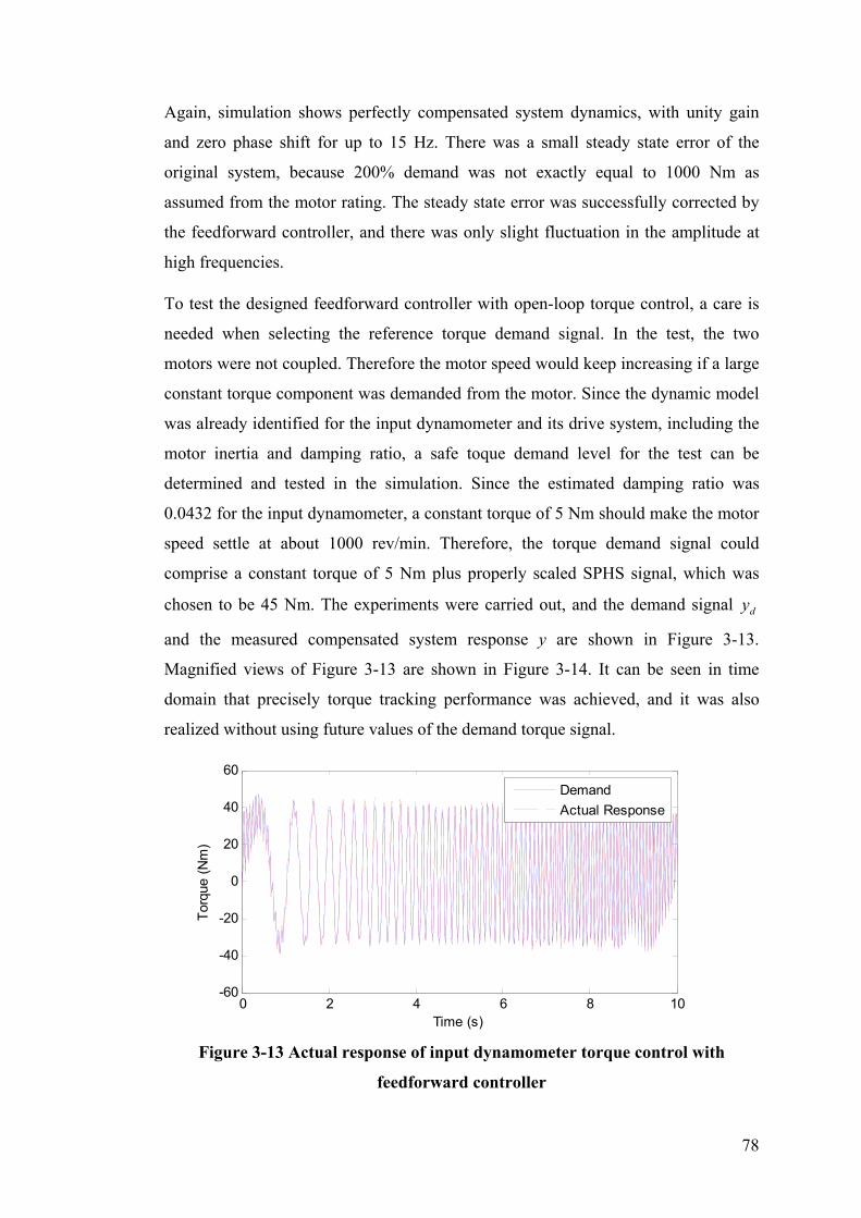
Again, simulation shows perfectly compensated system dynamics, with unity gain

and zero phase shift for up to 15 Hz. There was a small steady state error of the

original system, because 200% demand was not exactly equal to 1000 Nm as

assumed from the motor rating. The steady state error was successfully corrected by

the feedforward controller, and there was only slight fluctuation in the amplitude at

high frequencies.

To test the designed feedforward controller with open-loop torque control, a care is

needed when selecting the reference torque demand signal. In the test, the two

motors were not coupled. Therefore the motor speed would keep increasing if a large

constant torque component was demanded from the motor. Since the dynamic model

was already identified for the input dynamometer and its drive system, including the

motor inertia and damping ratio, a safe toque demand level for the test can be

determined and tested in the simulation. Since the estimated damping ratio was

0.0432 for the input dynamometer, a constant torque of 5 Nm should make the motor

speed settle at about 1000 rev/min. Therefore, the torque demand signal could

comprise a constant torque of 5 Nm plus properly scaled SPHS signal, which was

chosen to be 45 Nm. The experiments were carried out, and the demand signal yd

and the measured compensated system response y are shown in Figure 3-13.

Magnified views of Figure 3-13 are shown in Figure 3-14. It can be seen in time

domain that precisely torque tracking performance was achieved, and it was also

realized without using future values of the demand torque signal.

0 2 4 6 8 10 Time (s)

Figure 3-13 Actual response of input dynamometer torque control with

feedforward controller

-60

-40

-20

0

20

40

60

Tor

que

(Nm

)

Demand

Actual Response

78

50 60 60

40 40 40

3020 20

20

0 010

-20 -20 0

-10 -40 -40 0 0.2 0.4 5 5.2 5.4 9 9.2 9.4

Time (s)

Figure 3-14 Magnified views of Figure 3-13

Tor

que

(Nm

)

The frequency response of open-loop torque control of input dynamometer with and

without the feedforward controller is shown in Figure 3-15.

-15

-10

-5

0

5

Am

plitu

de (

dB)

-1 0 110 10 10

10-1

100

101

-600

-400

-200

0

200

Pha

se (

Deg

)

Only Feedback Control

With Feedforward Control

Frequency (Hz)

Figure 3-15 Frequency response of Figure 3-13

The frequency domain results illustrate the amplitude and phase are well

compensated, although the results are not as good as in the simulation. These can be

attributable to the nonlinearity and estimation errors. Fluctuations in the low

frequency range for both original and compensated systems were due to

measurement errors. Similar to the speed control results, the torque response leads

79

the torque demand signal by a half of sampling time, which may be due to the zero

order hold approximation used in the digitalization of the estimated transfer function.

3.4 Conclusions

Excellent tracking was achieved by using the proposed causal digital preview filter

as feedforward controller in both speed and torque control of the output and input

dynamometers respectively.

The causality was achieved by adding manual delays to the original system after the

actual response signal. Then the non-causal feedforward controller was designed for

the delayed output signal, rather than the actual signal. If the total sampling delays

between the delayed signal and actual signal can be made equal to the preview steps

required by the non-causal feedforward controller, the actual response will exactly

follow the demand signal without any delay. In that case the feedforward controller

can be deemed as a causal controller and can be implemented to both motor speed

and torque control when testing CVTs. Both simulation and experimental results are

presented to demonstrate the effectiveness of the proposed control method.

The digital preview filter is one of the available techniques to design feedforward

controllers. However, the proposed method can be applied to any other feedforward

controller technique to make the controller causal. One of the reasons that DPF was

implemented in this project was that a frequency domain weighting function can be

incorporated into the optimization to emphasize a frequency range of interests. In this

chapter, the weighting function was chosen to be uniform i.e. equal to one, over the

frequency range up to 15 Hz. When the controller was designed to be used in CVT

testing, the weighting function can be modified to emphasize good performance on a

certain frequency range determined by the simulation results based on the real-time

models.

The digital preview filter is designed to work within a defined frequency range.

Hence, to implement the feedforward controller in the test, it was necessary to test

the system with a reference signal, which does not include any frequency

components higher than the design bandwidth. Normally, a low pass filter should be

80

employed for the reference signal when testing the CVT with real-time engine and

vehicle models.

Another aspect of designing a feedforward controller was the selection of the

sampling frequency. The fastest sampling frequency of 160 Hz was used in the tests.

Using a lower sampling frequency in CP CADET, e.g. 80 Hz, would increase the

time delay on the CAN bus, and it also made the stabilization of the system much

harder by retuning the PID controller. Therefore the number of sampling delays that

can be added to the feedback loop is reduced. This meant that fewer preview steps

were available to design the digital preview filter, which could degenerate the

compensation performance. For example, with 80 Hz control frequency, only 4

manual delays could be added to the feedback loop giving the same absolute time

delay as 8 manual delays with 160 Hz control frequency, but the number of preview

steps available to design the feedforward controller was halved. This would certainly

degenerate the compensation performance.

81

Chapter 4

Feedforward Controller Robustness

Using a digital preview filter as part of a feedforward controller was demonstrated to

be effective in the previous chapter, but the feedforward controller was sensitive to

changes in the plant dynamics. It is not a problem for the generated torque control of

the input dynamometer, as it is open-loop control and the dynamics of the motor and

drive system is not affected by the other motor. However, for the output

dynamometer speed control, not only the gear ratio change will result in the change

of system dynamics, but also the torque generated by the input dynamometer will be

perceived as a disturbance by the output dynamometer.

One way to tackle the problem of changing system dynamics is to make the

feedforward controller adaptive to the plant dynamics. The plant dynamics could be

continuously estimated on-line, and the feedforward controller parameters could be

adjusted according to the updated system transfer function. The drawback of this

kind of control scheme is that the estimation process will take finite duration before

it converges, so it requires that the plant dynamics can only be slowly changing.

Because the continuous change in the CVT gear ratio will result in fast changing

closed loop dynamics, the performance of adaptive feedforward control may not be

satisfactory.

Another way would be to ensure that the original system dynamics is the same as the

one when the feedforward controller was designed. To achieve this, another

compensator is added to the system to retain the original system dynamics when the

gear ratio changes. The disturbance torque introduced by the input dynamometer is

also compensated by demanding additional percentage control signal from the output

dynamometer. In theory, the proposed gear ratio compensator can be updated at the

feedforward controller sampling rate or even faster, which is an advantage over the

existing adaptive method.

82

4.1 Gear Ratio Compensation of O/P Dynamometer

Speed Control

The feedforward controller was designed in the last chapter according to the

dynamics of the existing system, to approximate the inverse of the original system. It

is only effective when the dynamics of original system is kept unchanged. In the case

of speed control for the output dynamometer as shown in Figure 3-1, although the

PID controller, motor and drive system dynamics are invariant, the load dynamics in

terms of inertia and damping will vary with the gear ratio, when they are lumped into

the output dynamometer dynamics by the square of the ratio. Thus the feedforward

controller will fail to compensate the system dynamics if the gear ratio changes. This

can be solved in two ways, either updating the feedforward controller to match the

new system dynamics as a result of the gear ratio change, or updating the closed loop

to compensate the change in gear ratio. As discussed at the beginning of the chapter,

the latter would be a better choice, which can be achieved by adding another

controller to the feedback loop of the original system as shown in Figure 4-1.

PID Controller

PIDController

Motor & Drive System

Motor & Drive System

LoadLoad+

-

Speed SP Speed Percentage Torque

Gear Ratio Compensator

Gear Ratio Compensator

Figure 4-1 Output dynamometer closed loop speed control with gear ratio

compensator

The purpose of the gear ratio compensator is to retain the dynamics of the original

system when the gear ratio changes. The compensator can be formulated as follows:

GRatio _ cmp (s) (JO

2 J I )s (BO 2 BI ) (4-1)

J N s BN

where is the gear ratio. J I and BI are the combined inertia and damping ratio of

the input dynamometer and input shaft, and JO and BO are the combined inertia and

damping ratio of the output dynamometer and output shaft. J N and B N are the

nominal inertia and damping ratio of a virtual load, on which the feedforward

83

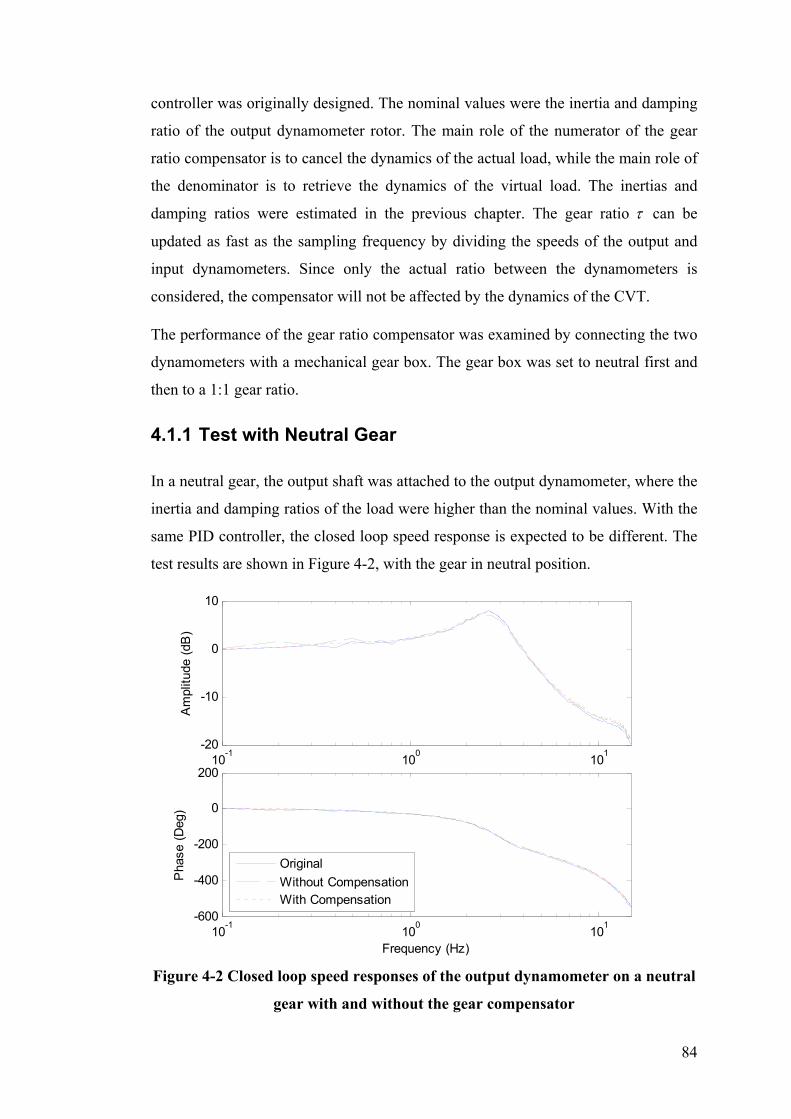
controller was originally designed. The nominal values were the inertia and damping

ratio of the output dynamometer rotor. The main role of the numerator of the gear

ratio compensator is to cancel the dynamics of the actual load, while the main role of

the denominator is to retrieve the dynamics of the virtual load. The inertias and

damping ratios were estimated in the previous chapter. The gear ratio can be

updated as fast as the sampling frequency by dividing the speeds of the output and

input dynamometers. Since only the actual ratio between the dynamometers is

considered, the compensator will not be affected by the dynamics of the CVT.

The performance of the gear ratio compensator was examined by connecting the two

dynamometers with a mechanical gear box. The gear box was set to neutral first and

then to a 1:1 gear ratio.

4.1.1 Test with Neutral Gear

In a neutral gear, the output shaft was attached to the output dynamometer, where the

inertia and damping ratios of the load were higher than the nominal values. With the

same PID controller, the closed loop speed response is expected to be different. The

test results are shown in Figure 4-2, with the gear in neutral position.

-1 0 110 10 10

-1 0 110 10 10

Frequency (Hz)

Figure 4-2 Closed loop speed responses of the output dynamometer on a neutral

gear with and without the gear compensator

-20

-10

0

10

Am

plitu

de (

dB)

-600

-400

-200

0

200

Pha

se (

Deg

)

Original

Without Compensation With Compensation

84

-10

-5

0

5

10

Am

plitu

de (

dB)

010

1 2 3 4 5 -300

-200

-100

0

Pha

se (

Deg

)

Original

Without Compensation With Compensation

Frequency (Hz)

Figure 4-3 A magnified view of Figure 4-2

The solid line shows the closed loop speed response of only output dynamometer

with added manual delays as in previous chapter in Figure 3-3. With a neutral gear

ratio and the output shaft attached, and the same PID controller parameters there was

only slight change in the amplitude, and the phase was almost the same as before,

because the inertia and damping of the output shaft is relatively small compared to

the output dynamometer. However, deviation from original dynamics can still be

observed in the amplitude, especially in the middle frequency range, between 2 Hz

and 4 Hz as shown in Figure 4-3. This was successful corrected by the gear ratio

compensator, as shown by the dotted line.

If the feedforward controller designed in previous chapter was used here without any

change in its parameters, the nominal load used in the gear ratio compensator would

be the inertia and damping of the output dynamometer rotor. The speed demand

consisted of a SPHS signal with a frequency range of up to 15 Hz and a scaled

amplitude of 45 rev/min, superposed on a steady state speed of 1000 rev/min. The

test results in the time domain are shown in Figure 4-4. Magnified views of Figure

4-4 are shown in Figure 4-5.

85

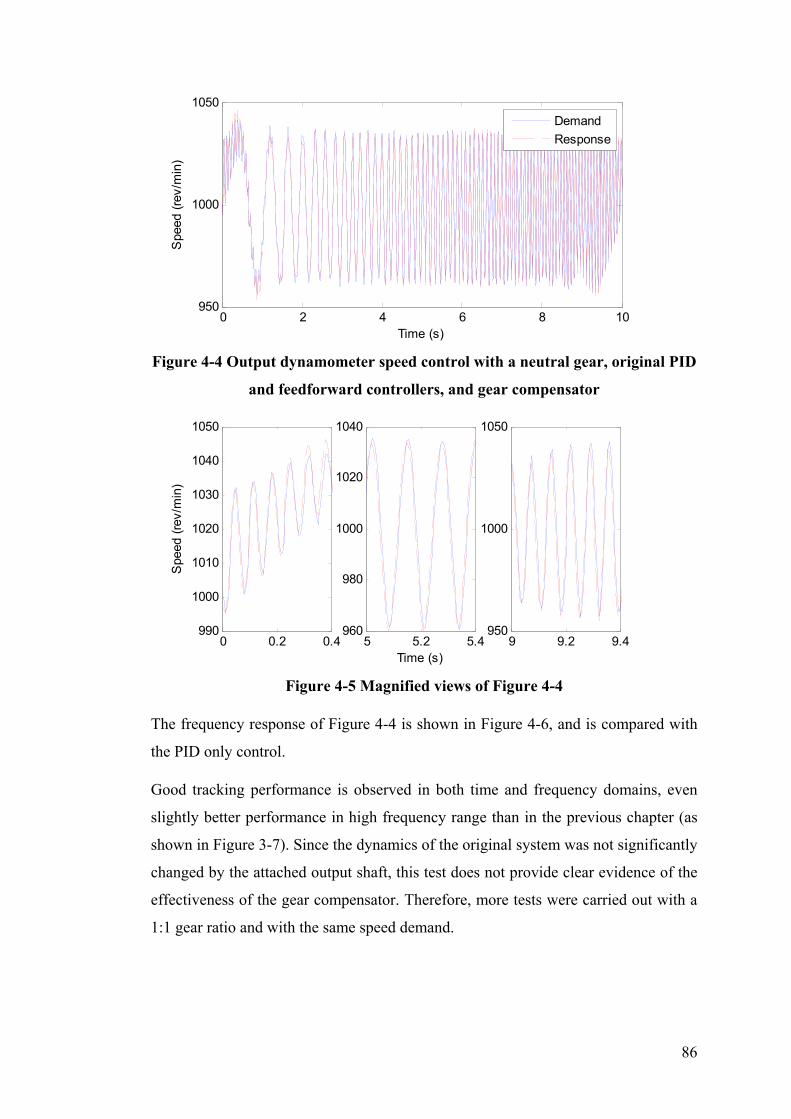
0 2 4 6 8 10 950

1000

1050

Spe

ed (

rev/

min

)

Demand

Response

Time (s)

Figure 4-4 Output dynamometer speed control with a neutral gear, original PID

and feedforward controllers, and gear compensator

990

1000

1010

1020

1030

1040

1050

Spe

ed (

rev/

min

)

960

980

1000

1020

1040

950

1000

1050

0 0.2 0.4 5 5.2 5.4 9 9.2 9.4 Time (s)

Figure 4-5 Magnified views of Figure 4-4

The frequency response of Figure 4-4 is shown in Figure 4-6, and is compared with

the PID only control.

Good tracking performance is observed in both time and frequency domains, even

slightly better performance in high frequency range than in the previous chapter (as

shown in Figure 3-7). Since the dynamics of the original system was not significantly

changed by the attached output shaft, this test does not provide clear evidence of the

effectiveness of the gear compensator. Therefore, more tests were carried out with a

1:1 gear ratio and with the same speed demand.

86

-20

-10

0

10

Am

plitu

de (

dB)

-1 0 110 10 10

10-1

100

101

-600

-400

-200

0

200

Pha

se (

Deg

)

PID Control

Feedforward control

Frequency (Hz)

Figure 4-6 Frequency response of Figure 4-4

4.1.2 Test with 1:1 Gear Ratio

With the gear ratio set to 1:1, the responses of the closed loop PID speed control with

and without the gear compensator are shown in Figure 4-7, and compared with the

original system response of only the output dynamometer.

The solid line still shows the closed loop speed response of only output dynamometer.

With a 1:1 gear ratio and the whole shaft including input dynamometer rotor attached

to the output dynamometer, the closed loop speed response was significantly

changed, as shown by the dashed line. With the gear compensator, the frequency

response was successfully compensated to give the same response as the original

system, as shown by the dotted line. It can be seen that perfect match was achieved

for both amplitude and phase for the frequencies up to 6 Hz. Within this frequency

range, the dynamics of the system with a 1:1 gear ratio was successfully made to

match the original system by the gear compensator. Large discrepancies at high

frequencies are due to the backlash between the gears, which were heard when

running the motor in high frequency range.

87

-30

-20

-10

0

10

Am

plitu

de (

dB)

-1 0 110 10 10

-600

-400

-200

0

200

Pha

se (

Deg

)

Original

Without Compensation With Compensation

-1 0 110 10 10

Frequency (Hz)

Figure 4-7 Closed loop speed control dynamics of output dynamometer with a

1:1 gear ratio

Since the compensated system with a 1:1 gear ratio matches the original system for

frequencies only up to 6 Hz without noticeable effects of backlash, tests were carried

out with a SPHS speed demand signal with frequency components up to 10 Hz. The

test results are shown in Figure 4-8. Magnified views of Figure 4-8 are shown in

Figure 4-9.

960

980

1000

1020

1040

Spe

ed (

rev/

min

)

Demand

Response

0 2 4 6 8 10 Time (s)

Figure 4-8 Output dynamometer speed control with a 1:1 gear ratio, original

PID and feedforward controllers, and gear compensator

88

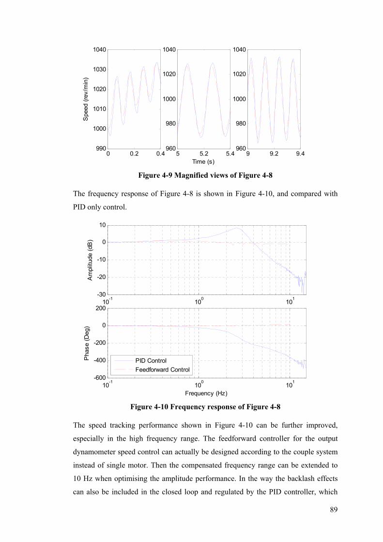
1040 1040 1040

1030 1020 1020

1020

1000 1000

1010

980 980 1000

990 960 960 0 0.2 0.4 5 5.2 5.4 9 9.2 9.4

Time (s)

Figure 4-9 Magnified views of Figure 4-8

Spe

ed (

rev/

min

)

The frequency response of Figure 4-8 is shown in Figure 4-10, and compared with

PID only control.

-30

-20

-10

0

10

Am

plitu

de (

dB)

-1 0 110 10 10

10-1

100

101

-600

-400

-200

0

200

Pha

se (

Deg

)

PID Control

Feedforward Control

Frequency (Hz)

Figure 4-10 Frequency response of Figure 4-8

The speed tracking performance shown in Figure 4-10 can be further improved,

especially in the high frequency range. The feedforward controller for the output

dynamometer speed control can actually be designed according to the couple system

instead of single motor. Then the compensated frequency range can be extended to

10 Hz when optimising the amplitude performance. In the way the backlash effects

can also be included in the closed loop and regulated by the PID controller, which

89

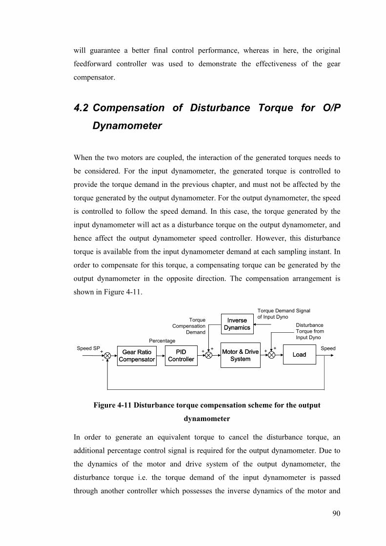
will guarantee a better final control performance, whereas in here, the original

feedforward controller was used to demonstrate the effectiveness of the gear

compensator.

4.2 Compensation of Disturbance Torque for O/P

Dynamometer

When the two motors are coupled, the interaction of the generated torques needs to

be considered. For the input dynamometer, the generated torque is controlled to

provide the torque demand in the previous chapter, and must not be affected by the

torque generated by the output dynamometer. For the output dynamometer, the speed

is controlled to follow the speed demand. In this case, the torque generated by the

input dynamometer will act as a disturbance torque on the output dynamometer, and

hence affect the output dynamometer speed controller. However, this disturbance

torque is available from the input dynamometer demand at each sampling instant. In

order to compensate for this torque, a compensating torque can be generated by the

output dynamometer in the opposite direction. The compensation arrangement is

shown in Figure 4-11.

PID Controller

PIDController

Motor & Drive System

Motor & Drive System

LoadLoad+

-

Speed SP Speed

Percentage

Disturbance Torque from Input Dyno

++

Torque Compensation

Demand

+ +

Inverse Dynamics

Inverse Dynamics

Torque Demand Signal of Input Dyno

Gear Ratio Compensator

Gear Ratio Compensator

Figure 4-11 Disturbance torque compensation scheme for the output

dynamometer

In order to generate an equivalent torque to cancel the disturbance torque, an

additional percentage control signal is required for the output dynamometer. Due to

the dynamics of the motor and drive system of the output dynamometer, the

disturbance torque i.e. the torque demand of the input dynamometer is passed

through another controller which possesses the inverse dynamics of the motor and

90

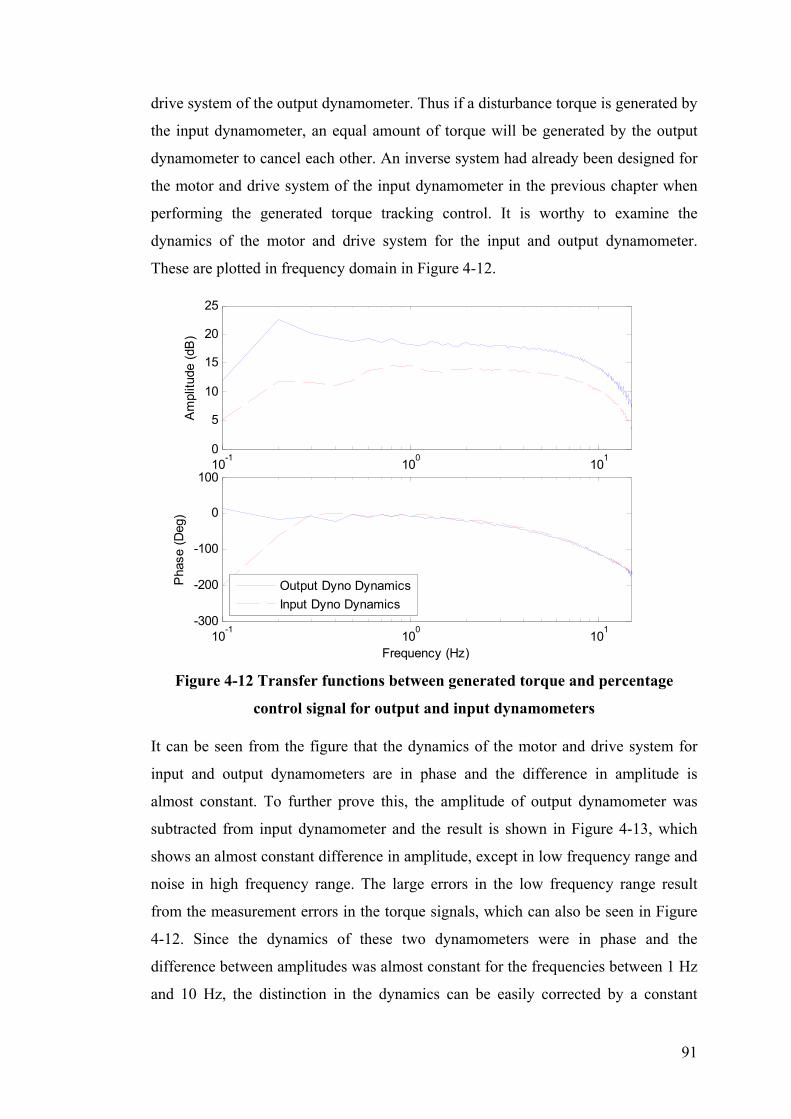
drive system of the output dynamometer. Thus if a disturbance torque is generated by

the input dynamometer, an equal amount of torque will be generated by the output

dynamometer to cancel each other. An inverse system had already been designed for

the motor and drive system of the input dynamometer in the previous chapter when

performing the generated torque tracking control. It is worthy to examine the

dynamics of the motor and drive system for the input and output dynamometer.

These are plotted in frequency domain in Figure 4-12.

0

5

10

15

20

25

Am

plitu

de (

dB)

-1 0 110 10 10

10-1

100

101

-300

-200

-100

0

100

Pha

se (

Deg

)

Output Dyno Dynamics

Input Dyno Dynamics

Frequency (Hz)

Figure 4-12 Transfer functions between generated torque and percentage

control signal for output and input dynamometers

It can be seen from the figure that the dynamics of the motor and drive system for

input and output dynamometers are in phase and the difference in amplitude is

almost constant. To further prove this, the amplitude of output dynamometer was

subtracted from input dynamometer and the result is shown in Figure 4-13, which

shows an almost constant difference in amplitude, except in low frequency range and

noise in high frequency range. The large errors in the low frequency range result

from the measurement errors in the torque signals, which can also be seen in Figure

4-12. Since the dynamics of these two dynamometers were in phase and the

difference between amplitudes was almost constant for the frequencies between 1 Hz

and 10 Hz, the distinction in the dynamics can be easily corrected by a constant

91

scaling factor, without the need to design an inverse dynamics compensator for the

output dynamometer. This factor was measured to be 0.636 for the frequencies

between 1 Hz and 10 Hz.

-1 0 110 10 10

Frequency (Hz)

Figure 4-13 Difference in amplitude response of motor and drive system for

input and output dynamometers

Therefore the compensation torque of the disturbance from the input dynamometer

on the output dynamometer speed control can be structured as shown in Figure 4-14.

Input Dynamometer

-15

-10

-5

0

5 G

ain

(dB

)

+ +PID Controller

PID Controller

LoadLoad+

-

Speed SP Speed

Percentage Disturbance Torque

- +

0.6360.636

Input Dynamometer

Input Dynamometer

Torque SP Torque

ScalarScalar

Output Dynamometer

Output Dynamometer

Percentage

Feedforward Controller

FeedforwardController

Feedforward Controller

FeedforwardController

Gear Ratio Compensator

Gear RatioCompensator

CVT

Figure 4-14 Block diagram of torque compensation scheme for output

dynamometer speed control

To verify the proposed compensation scheme, both dynamometers were switched on.

The output dynamometer was in speed control and input dynamometer was in torque

control. Both feedforward controllers were kept the same as designed in the previous

chapter. The output dynamometer speed demand consisted of a DC speed of 1000

rev/min plus a SPHS signal with a frequency range of up to 10 Hz, and a scaled

amplitude to 35 rev/min. The input dynamometer torque demand consisted of a

92

SPHS signal with the same frequency range and amplitude. The test results are

shown in the following figures.

The measured output dynamometer speed is shown in Figure 4-15. Magnified views

of Figure 4-15 are shown in Figure 4-16.

Time (s)

Figure 4-15 Output dynamometer speed with a 1:1 gear ratio

1040 1040 1040

1030 1020 1020

1020

1000 1000

1010

980 9801000

990 960 960 0 0.2 0.4 5 5.2 5.4 9 9.2 9.4

Time (s)

Figure 4-16 Magnified views of Figure 4-15

The frequency response of the system was shown in Figure 4-17, compared with the

one without a torque disturbance, when the input dynamometer was switched off.

0 2 4 6 8 10 960

980

1000

1020

1040

Spe

ed (

rev/

min

)

Demand

Response

Spe

ed (

rev/

min

)

93

-10

-5

0

5

10

Am

plitu

de (

dB)

-1 0 110 10 10

10-1

100

101

-100

-50

0

50

100

Pha

se (

Deg

)

Without Torque Disturbance

With Torque Disturbance

Frequency (Hz)

Figure 4-17 Frequency response of Figure 4-15 compared with the results shown

in Figure 4-10

It can be seen that the speed was well controlled. If comparing with the speed

response without external torque in Figure 4-10, the results were quite similar to each

other, which verified the effectiveness of the disturbance torque compensation

scheme for the output dynamometer. The compensation scheme was based on the

differences between the dynamics the input and output dynamometers, as seen in

Figure 4-13. The difference in amplitude response was not perfectly flat. The

compensation factor used here was an averaged value, so there was a small

discrepancy for the two speed control responses in the amplitude at high frequencies

as shown in Figure 4-17. In other words, the speed control was still affected by the

torque generated by the input dynamometer, but in a negligible way. The phase

response was also delayed, but seemed to offer a better result. Difference in the

responses at high frequencies with and without torque disturbance could result from

the backlash effect. With the backlash between the gears, the torque generated by the

input dynamometer will not be immediately cancelled by the torque generated by the

output dynamometer, even if the compensation factor was accurate.

The proposed scheme is based on the dynamics difference of the dynamometers. It

eliminates the need to design an additional feedforward controller, and also it is

94

based on the control signal rather than the measured torque value, which may be

contaminated by significant noise.

The input dynamometer torque controller performance was also assessed by using

the data obtained from the same test. The generated input dynamometer torque is

shown in Figure 4-18, and compared with the torque demand. The generated torque

was calculated by using Equation (2-31). Magnified views of Figure 4-18 is shown in

Figure 4-19.

0 2 4 6 8 10 -40

-20

0

20

40

Tor

que

(Nm

)

Demand

Response

Time (s)

Figure 4-18 Demanded and generated input dynamometer torque with a 1:1

gear ratio

40 40 60

30 20 30

Tor

que

(Nm

)

20

0 0

10

-20 -300

-10 -40 -60 0 0.2 0.4 5 5.2 5.4 9 9.2 9.4

Time (s)

Figure 4-19 Magnified views of Figure 4-18

The frequency response of the torque control system is shown in Figure 4-20.

95

Pha

se (

Deg

) A

mpl

itude

(dB

)

10

5

0

-5

-10 -1 0 1

10 10 10100

50

0

-50

-100 -1 0 1

10 10 10Frequency (Hz)

Figure 4-20 Frequency response of Figure 4-18

It can be seen from both time and frequency domain results that the generated input

dynamometer torque was precisely controlled to track the torque demand, and was

not affected by the coupling between the input and output dynamometers. A similar

result to the one on single motor control as shown in previous chapter in Figure 3-15

was obtained. The control result was almost perfect except for the small error in high

frequency, which was also seen in Figure 3-15.

4.3 Compensation of Inertia Torque for I/P

Dynamometer

So far, the generated torque of the input dynamometer was controlled to track the

torque demand, without jeopardising the speed control of the output dynamometer.

When testing a CVT in a real vehicle, the torque applied on the input shaft of the

CVT is the engine brake torque. Since the input shaft of the CVT was connected to

the input dynamometer where the torque measurement was taken, it would be more

realistic that the measured input dynamometer torque was controlled to track the

simulated engine brake torque rather than the generated torque.

96

The difference between the generated torque and measured torque was the torque

used to accelerate the input dynamometer rotor inertia and to overcome the damping

inside the motor. This difference needs to be compensated to make the measured

torque track the torque demand. Since the inertia and damping ratio had already been

estimated for the input dynamometer in Chapter 2, they can be compensated by

calculating the acceleration from the output dynamometer speed demand, the inertia

and damping compensation scheme is shown in Figure 4-21.

+ +PID Controller

PIDController

LoadLoad+

-

Speed SP Speed

Percentage

Disturbance Torque

- +

0.6360.636

Input Dynamometer

Input Dynamometer

Torque

ScalarScalar

Output Dynamometer

OutputDynamometer

Percentage Torque SP

Inertia&Friction Compensation Inertia&FrictionCompensation

+

+

Feedforward Controller

FeedforwardController

Feedforward Controller

FeedforwardController

Gear Ratio Compensator

Gear RatioCompensator

CVT

Output Dynamometer

Figure 4-21 Inertia and damping torque compensation scheme for input

dynamometer

Theoretically, the inertia and damping torque should be calculated from the

measured speed response of the input dynamometer rather than the speed demand,

but the measured speed contains noise and results in large errors when calculating the

derivative. More importantly, it will introduce high frequency input signal to the

feedforward controller of the torque control, which was designed for a specific

frequency range. With near perfect speed control, the compensation calculated from

the speed demand should give the same results as the one calculated from the actual

speed.

4.3.1 Test with Inertia Torque Compensator

Tests were carried out to examine the proposed inertia and damping compensation

scheme. The speed demand for the output dynamometer was the same as before. The

torque demand for the input dynamometer consisted of a SPHS signal with

frequencies up to 10 Hz and an amplitude of 45 Nm, superposed on a steady state of

97

torque demand of 100 Nm. The measured input dynamometer torque is shown in

Figure 4-22. Magnified views of Figure 4-22 are shown in Figure 4-23.

20

60

100

140

180 T

orqu

e (N

m)

Demanded

Measured

0 2 4 6 8 10 Time (s)

Figure 4-22 Measured torque of input dynamometer with inertia torque

compensation

160 160 160

150 140 140

140120 120

Tor

que

(Nm

)

130 100 100

120

80 80110

60 60100

90 40 40 0 0.2 0.4 5 5.2 5.4 9 9.2 9.4

Time (s)

Figure 4-23 Magnified view of Figure 4-22

The frequency response is shown in Figure 4-24. It can be seen from the test results

in both time and frequency domains that although the inertia and damping torque

compensation for input dynamometer was simple, the compensation method is

extremely effective. The amplitude of the measured torque in the middle frequency

range was slightly higher than the demand. This could be due to the error in the

output dynamometer speed control. As discussed, the error in speed control will lead

to the errors in the calculation of inertia and damping torque.

98

-10

-5

0

5

10

Am

plitu

de (

dB)

-1 0 110 10 10

-1 0 110 10 10

Frequency (Hz)

Figure 4-24 Frequency response of Figure 4-22

-100

-50

0

50

100

Pha

se (

Deg

)

To further examine this, the speed response of the output dynamometer was also

recorded, and the response in time domain is shown in Figure 4-25. Magnified views

of Figure 4-25 is shown in Figure 4-26. The frequency response is shown in Figure

4-27.

940

960

980

1000

1020

1040

1060

Spe

ed (

rev/

min

)

Demanded

Response

0 2 4 6 8 10Time (s)

Figure 4-25 Speed response of output dynamometer with inertia torque

compensation for input dynamometer

99

1040 1040 1040

1030 1020 1020

1020

1000 1000

1010

980 980 1000

990 960 960 0 0.2 0.4 5 5.2 5.4 9 9.2 9.4

Time (s)

Figure 4-26 Magnified views of Figure 4-25

Spe

ed (

rev/

min

)

-10

-5

0

5

10

Am

plitu

de (

dB)

-1 0 110 10 10

10-1

100

101

-100

-50

0

50

100

Pha

se (

Deg

)

Frequency (Hz)

Figure 4-27 Frequency response of Figure 4-25

The output dynamometer speed performance shows errors in the middle frequency

range. The backlash effect is always one of the factors that affect the control

performance. Due to the backlash, even with a 1:1 gear ratio, the speed and torque

will be different on the input and output shafts. Then the disturbance torque from the

input dynamometer will not be exactly cancelled by the additional output

dynamometer torque even though an exactly same among of torque is generated in

the opposite direction. The speed of input dynamometer will also be different from

the speed of output dynamometer. The calculation of inertia and damping torque

100

from speed demand will not be the same as calculated from the input dynamometer

speed response even though the output dynamometer speed is equal to the speed

demand.

4.3.2 Test with additional PID controllers

The control performance could be further improved if another PID controller is

added for both output and input dynamometer controls on the outer loop to further

correct the tracking error. Then the speed control will be in the form of structure (a)

in Figure 1-9, and the torque control will be in the form of structure (b) in Figure 1-8.

The overall block diagram with additional PID controllers is shown in Figure 4-28.

+

++

+

+ +PID Controller

PIDController

LoadLoad+

-

Percentage Disturbance Torque

- +

0.636

Input Dynamometer

Input Dynamometer

Torque

ScalarScalar

Output Dynamometer

Ou

sationsat

tputDynamometer

Percentage

Torque SP

Inertia&Friction CompenInertia&FrictionCompen ion

-

+

PID Controller

PIDController

PID Controller

PID Controller

+

-

+

Feedforward Controller

FeedforwardController

Feedforward Controller

Feedforward Controller

Gear Ratio Compensator

Gear Ratio Compensator

CVT

Speed SP Speed

Figure 4-28 Overall control block diagram with additional PIDs

Tuning of the PID controller would be dependent on a specific application. If the

feedforward controls for the motor torque and speed were nearly perfect, the torque

and speed errors would be very small, and the added PID controllers will have minor

effects on the original control systems. If the control errors were relatively large, the

PID controllers will provide further correction on the errors. But using additional

PID controllers will certainly introduce phase shift into the system, so better

performance can not be guaranteed. Sometimes a compromise may need to be

considered for the amplitude and phase when tuning the parameters of the PID

controller.

Tests were carried out with the same speed and torque demand for the output and

input dynamometers as the previous test. Two more PID controllers were added to

101

the outer loop of the speed and torque control. The PID parameters were tuned in

dSPACE starting with 0.1 for both proportional and integral gains. The derivative

gain was set to be 0 due to the noise. Then by running the test through SPHS cycles,

the gains were adjusted to offer better time responses. Finally, the PID parameters for

the speed control were tuned to be 0.08 for the proportional gain, 0.4 for the integral

gain and 0 for the derivative gain, while for the torque control the parameters were

0.03 for the proportional gain, 0.3 for the integral gain and 0 for the derivative gain.

With additional PID controllers, the measured input dynamometer torque is shown in

Figure 4-29. Magnified views of Figure 4-29 is shown in Figure 4-30. The frequency

response is shown in Figure 4-31, compared with the response without additional

PID controller.

20

40

60

80

100

120

140

160

180

Tor

que

(Nm

)

Demanded

Measured

0 2 4 6 8 10 Time (s)

Figure 4-29 Measured input dynamometer torque with additional PID

controller

160 150 160

150 140

140120

Tor

que

(Nm

)

130 100 100

120

80110

60100

90 50 40 0 0.2 0.4 5 5.2 5.4 9 9.2 9.4

Time (s)

Figure 4-30 Magnified views of Figure 4-29

102

-10

-5

0

5

10

Am

plitu

de (

dB)

-1 0 110 10 10

10-1

100

101

-100

-50

0

50

100

Pha

se (

Deg

)

Original

With Additional PID

Frequency (Hz)

Figure 4-31 Frequency response of Figure 4-29 compared with the results shown

in Figure 4-24

It can be seen from the amplitude response that the tracking error was reduced,

especially in the middle frequency range. Meanwhile, the phase became slightly

worse at the same frequency range. As discussed before, the PID controller will

introduce phase shift into the system, and sometimes it is a compromise between

amplitude and phase responses. However, the control results were already

satisfactory without the additional PID controller, i.e. the additional PID controller

did not show much improvement.

Relatively large control errors were observed on the output dynamometer speed

control response in Figure 4-27. The response is significantly improved by the

additional PID controller. The time domain response is shown in Figure 4-32.

Magnified views of Figure 4-32 are shown in Figure 4-33. The frequency response is

shown in Figure 4-34 compared with the response without additional PID controller.

Comparing Figures 4-25 and 4-32, the improvement in time domain is very obvious

between 1 s and 3 s. In frequency domain, a definitely better result was observed for

both amplitude and phase up to 2 Hz, due to the use of the PI controller, which has

more effects in the low frequency range. Fluctuation occurs around 3 Hz for both

amplitude and phase response, which was also observed in the torque control in

103

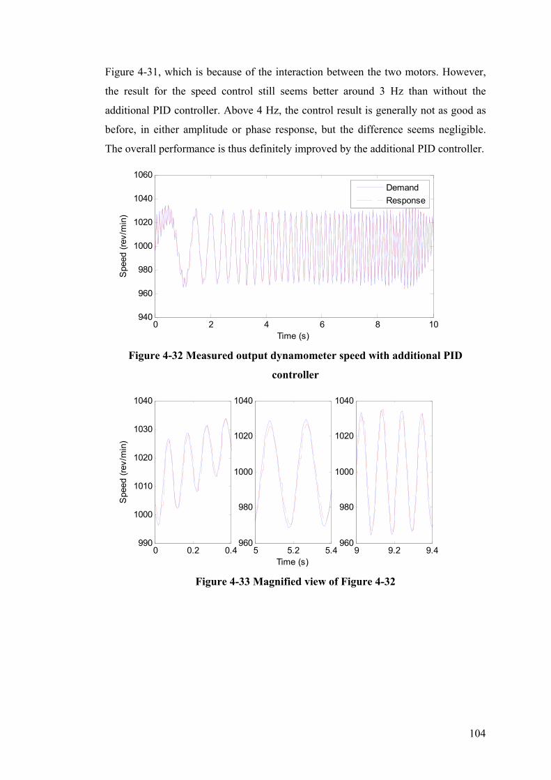
Figure 4-31, which is because of the interaction between the two motors. However,

the result for the speed control still seems better around 3 Hz than without the

additional PID controller. Above 4 Hz, the control result is generally not as good as

before, in either amplitude or phase response, but the difference seems negligible.

The overall performance is thus definitely improved by the additional PID controller.

0 2 4 6 8 10 940

960

980

1000

1020

1040

1060

Spe

ed (

rev/

min

)

Demand

Response

Time (s)

Figure 4-32 Measured output dynamometer speed with additional PID

controller

1040 1040 1040

1030 1020 1020

Spe

ed (

rev/

min

)

1020

1000 1000

1010

980 980 1000

990 960 960 0 0.2 0.4 5 5.2 5.4 9 9.2 9.4

Time (s)

Figure 4-33 Magnified view of Figure 4-32

104

-10

-5

0

5

10

Am

plitu

de (

dB)

-1 0 110 10 10

10-1

100

101

-100

-50

0

50

100

Pha

se (

Deg

)

Original

With Additional PID

Frequency (Hz)

Figure 4-34 Frequency response of Figure 4-32

Hence, the performance of the additional PID controller is hard to predict, especially

when the two motors are coupled. It could be a compromise on the performance

between amplitude and phase responses, like the input dynamometer torque control,

or between low and high frequency ranges, like the output dynamometer speed

control. The utilization of additional PID controller and tuning its parameters will

depend on the specific application. Normally the additional PID controller is not

necessary or the parameters can be set to be relatively small, so that it will only act

on relatively big errors. At the same time, it will not change the dynamics of the

original system and affect the performance of the feedforward controller.

105

Chapter 5 Testing with Real Time Model

All the previous tests were carried out with SPHS multi frequency signal as input.

Since it contains all the specified sub harmonics in one signal, it provides a

challenging way to test the effectiveness of the proposed torque and speed tracking

controllers, but this kind of signal was not expected when testing CVTs. More

realistic signals are used to test the designed controllers in this section, which are the

engine brake torque and vehicle speed simulated from real-time engine and vehicle

models. Although the real-time model is constructed with a manual transmission

rather than a CVT, the simulation results are still representing typical engine brake

torques and vehicle speeds encountered in real driving conditions.

5.1 Engine and Vehicle model

The engine and vehicle model used in this section of the work were supplied by the

Ford Motor company and for brevity and confidentiality reasons only their main

attributes are described here.

The vehicle model is based on the standard vehicle road load equation, including

speed dependent rolling resistance, aerodynamic drag, acceleration and gradient

effects. It can be expressed by the equation as follows:

Ft rcmv g mva mv g sin r 1 CD Avv

2 (5-1)2

The dynamics of tyre traction and stiffness and damping in the vehicle drive shafts

are also embedded within the model.

The engine model is termed as a ‘mean value engine model’, the outputs from the

model are the cycle averages for one complete engine cycle, as opposed to a crank

angle based model where outputs are derived on a crank angle basis and thus include

106

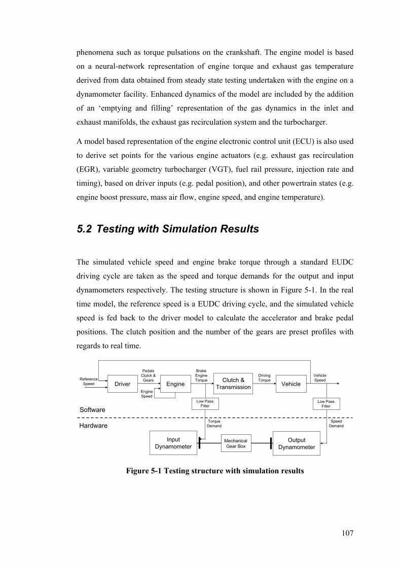
phenomena such as torque pulsations on the crankshaft. The engine model is based

on a neural-network representation of engine torque and exhaust gas temperature

derived from data obtained from steady state testing undertaken with the engine on a

dynamometer facility. Enhanced dynamics of the model are included by the addition

of an ‘emptying and filling’ representation of the gas dynamics in the inlet and

exhaust manifolds, the exhaust gas recirculation system and the turbocharger.

A model based representation of the engine electronic control unit (ECU) is also used

to derive set points for the various engine actuators (e.g. exhaust gas recirculation

(EGR), variable geometry turbocharger (VGT), fuel rail pressure, injection rate and

timing), based on driver inputs (e.g. pedal position), and other powertrain states (e.g.

engine boost pressure, mass air flow, engine speed, and engine temperature).

5.2 Testing with Simulation Results

The simulated vehicle speed and engine brake torque through a standard EUDC

driving cycle are taken as the speed and torque demands for the output and input

dynamometers respectively. The testing structure is shown in Figure 5-1. In the real

time model, the reference speed is a EUDC driving cycle, and the simulated vehicle

speed is fed back to the driver model to calculate the accelerator and brake pedal

positions. The clutch position and the number of the gears are preset profiles with

regards to real time.

Driver

Mechanical Gear Box

Clutch & Transmission Vehicle

Input Dynamometer

Output Dynamometer

Engine

Brake Engine Torque

Driving Torque

Vehicle Speed Reference

Speed

Pedals Clutch & Gears

Low Pass Filter

Torque Demand

Low Pass Filter

Speed Demand

Engine Speed

Software

Hardware

Figure 5-1 Testing structure with simulation results

107

The test results for the output dynamometer speed control are shown in Figure 5-2,

while the test results for the input dynamometer torque control are shown in Figure

5-3.

Since the EUDC driving cycle consists of several small driving cycles, the simulated

vehicle speed and engine brake torque also contains similar profiles for each

individual cycle. Typical acceleration and braking processes are selected for a

magnified view from Figure 5-2 for speed control, and shown in Figure 5-4.

Meanwhile, the same regions are also selected from Figure 5-3 for torque control,

magnified, and shown in Figure 5-5.

It can be seen from these test results that excellent tracking control was achieved for

both torque and speed. The tracking errors were generally due to noise. As motioned

before, the torque transducer has an accuracy of +/- 0.1% of full scale, i.e. +/- 1 Nm,

so the measurement error will have more effects at low torque values. There is also

some error from calibration of the torque transducer, e.g. it measuring between -1.2

and -0.8 Nm when the motors were switched off.

In fact, the simulated engine brake torque was not flat, e.g. between 250 s and 260 s

shown in Figure 5-5 (b), there were small variations in the amplitude of the signal,

which was normally less than 1 Nm, as shown in Figure 5-6. The feedforward

controller will attempt to follow these fast but low amplitude signals, but the

resultant response can not be accurately measured. This caused an error for the PID

controller to further correct, thus a noisy response in torque was observed.

The most critical aspect in the overall control was not the behaviour of the

feedforward controller, but the dynamic compensation for the output dynamometer

when the two motors were coupled, such that torque generated by the input

dynamometer will not have any effects on the output dynamometer. The speed

control compensation was achieved by a dynamics factor as shown in Figure 4-13,

which was almost constant, except for noise in the high frequency range. If the

compensation failed due to the inaccuracy of the dynamics factor, the speed of output

dynamometer will be pulled away from the speed demand by the input dynamometer

torque, and the compensation of inertia and damping torque for the measured input

dynamometer torque, which was calculated from the speed demand will also fail in

this case.

108

0 100 200 300 400 500 600 -200

0

200

400

600

800

1000

1200

Spe

ed (

rev/

min

)

Demanded Speed

Measured Speed

(a)

(b) (c)

Time (s)

Figure 5-2 Measured output dynamometer speed again simulated vehicle speed

109

0 100 200 300 400 500 600 -100

-50

0

50

100

150

200

Tor

que

(Nm

)

Demanded Torque

Measured Torque

(a) (b) (c)

Time (s)

Figure 5-3 Measured input dynamometer torque against simulated engine brake torque

110

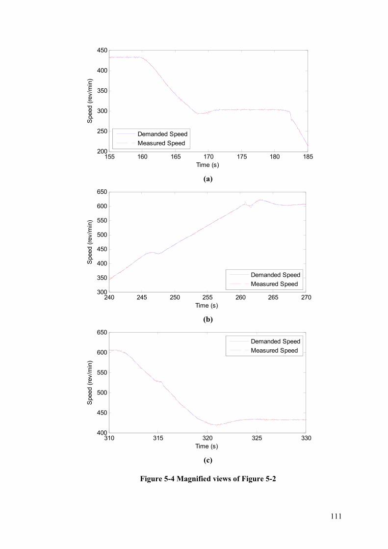
200

250

300

350

400

450

Spe

ed (

rev/

min

)

Demanded Speed

Measured Speed

155 160 165 170 175 180 185Time (s)

(a)

240 245 250 255 260 265 270Time (s)

(b)

310 315 320 325 330Time (s)

(c)

Figure 5-4 Magnified views of Figure 5-2

300

350

400

450

500

550

600

650

Spe

ed (

rev/

min

)

Demanded Speed

Measured Speed

400

450

500

550

600

650

Spe

ed (

rev/

min

)

Demanded Speed

Measured Speed

111

-60

-40

-20

0

20

40

60

Tor

uqe

(Nm

)

Demanded Torque

Measured Torque

155 160 165 170 175 180 185Time (s)

(a)

240 245 250 255 260 265 270Time (s)

(b)

310 315 320 325 330Time (s)

(c)

Figure 5-5 Magnified views of Figure 5-3

-50

0

50

100

150

200

Tor

uqe

(Nm

)

Demanded Torque

Measured Torque

-40

-20

0

20

40

60

80

Tor

uqe

(Nm

)

Demanded Torque

Measured Torque

112

254 254.5 255 255.5 256 93

94

95

96

97

98

99

100

Tor

uqe

(Nm

)

Demanded Torque

Measured Torque

Time (s)

Figure 5-6 Fluctuations in simulated engine brake torque as input dynamometer

torque demand

For example in Figures 5-4 (b) and 5-5 (b), there was a sudden drop in the brake

engine torque around 261 s because of a gear change and the associated lift off of the

accelerator pedal. As the dynamics compensation is not perfect, and the fast change

of the generated input dynamometer torque was not exactly repeated by the output

dynamometer in the opposite direction, the output dynamometer speed deviated from

the speed demand. Since the inertia torque was still calculated from the speed

demand, an error was caused on the measured input dynamometer torque. The error

in speed shown here was already improved by the additional PID controller, the

situation was worse before the PID controller was added.

When testing the CVT in a real vehicle, even with a robot driver, the speed tracking

accuracy needs to be within +/-1 km/h, i.e. +/-10 rev/min. The speed tracking error

shown in the test results is normally only +/-2 rev/min, and +/-10 rev/min on very

rare occasions, like shown in Figure 5-4 (b) around 261 s. When testing the CVT

with a real engine, the measured engine brake torque will also oscillate significantly

during an engine cycle for the firing and pumping processes, e.g. a peak value of 70

Nm for a mean brake torque of 30 Nm. The torque tracking error shown in the results

is normally +/-5 Nm, and +/-10 Nm for the worst situation. Hence, the control results

can sufficiently meet with the requirements to test a CVT.

In order to show the success of designed controllers for speed and torque control, a

new test was carried out on the input and output dynamometer running through the

simulation results, with the original PID controllers provided by the CP CADET

113

system. The test was only run up to 200 s, covering the first three small cycles. The

test results are shown in Figure 5-7 for measured output dynamometer speed and in

Figure 5-8 for measured input dynamometer torque.

0 50 100 150 200 -100

0

100

200

300

400

500 S

peed

(re

v/m

in)

Demanded Speed

Measured Speed

Time (s)

Figure 5-7 Measured output dynamometer speed with PID controllers in the CP

CADET system

0 50 100 150 200 -100

-50

0

50

100

150

Spe

ed (

rev/

min

)

Demanded Torque

Measured Torque

Time (s)

Figure 5-8 measured input dynamometer torque with PID controllers in the CP

CADET system

The same region as shown in Figures 5-4 (a) and 5-5 (a) was selected for a magnified

view, which is shown in Figures 5-9 and 5-10 for speed and torque control

respectively.

114

Time (s)

Figure 5-9 A magnified view of Figure 5-7

155 160 165 170 175 180 185 Time (s)

Figure 5-10 A magnified view of Figure 5-8

Because there is no compensation for the interaction between the two motors when

they are coupled, the PID controllers have to be tuned to emphasize good

performance on one control, either speed or torque. Otherwise the two PID

controllers will function against each other and damage the shaft. As seen from the

test results, the speed control was tuned to be stiff, and torque control to be loose. In

this case, the torque control performance is sacrificed, but even so the speed control

is still much worse than before as shown in Figure 5-4 (a). Moreover, the PID

controller is tuned for a specific gear ratio. Therefore, the performance will be worse

if the gear ratio changes.

As these results suggest, the proposed controllers improved the system response

significantly compared with the PID controllers as implemented by the manufacture

of the system. The interaction between these two motors was successfully

155 160 165 170 175 180 185 200

250

300

350

400

450

Spe

ed (

rev/

min

)

Demanded Speed

Measured Speed

-100

-50

0

50

100

Tor

que

(Nm

)

Demanded Torque

Measured Torque

115

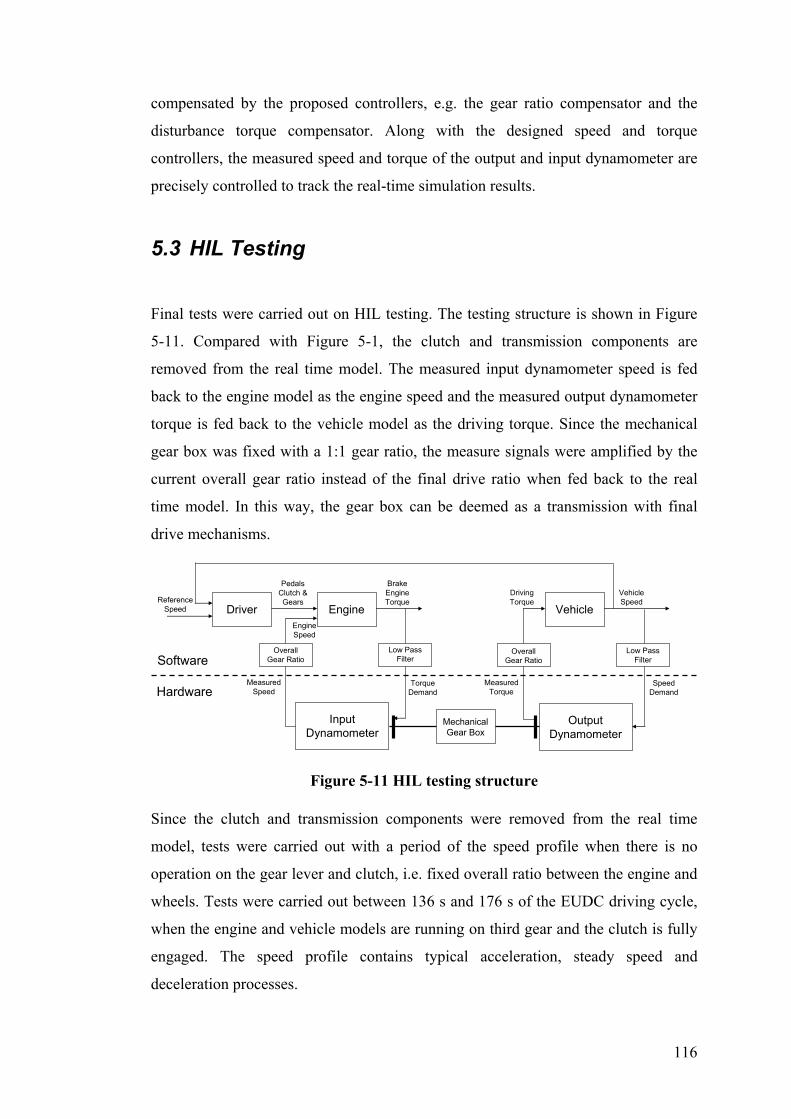
compensated by the proposed controllers, e.g. the gear ratio compensator and the

disturbance torque compensator. Along with the designed speed and torque

controllers, the measured speed and torque of the output and input dynamometer are

precisely controlled to track the real-time simulation results.

5.3 HIL Testing

Final tests were carried out on HIL testing. The testing structure is shown in Figure

5-11. Compared with Figure 5-1, the clutch and transmission components are

removed from the real time model. The measured input dynamometer speed is fed

back to the engine model as the engine speed and the measured output dynamometer

torque is fed back to the vehicle model as the driving torque. Since the mechanical

gear box was fixed with a 1:1 gear ratio, the measure signals were amplified by the

current overall gear ratio instead of the final drive ratio when fed back to the real

time model. In this way, the gear box can be deemed as a transmission with final

drive mechanisms.

Pedals Brake

Overall Gear Ratio

Low Pass Filter

Driver

Mechanical Gear Box

Vehicle

Input Dynamometer

Output Dynamometer

Engine

Torque Demand

Measured

Overall Gear Ratio

Speed Demand

Engine Speed

Measured Speed Torque

Low Pass Filter

Clutch & Engine Driving Vehicle Reference Speed Gears Torque Torque

Speed

Software

Hardware

Figure 5-11 HIL testing structure

Since the clutch and transmission components were removed from the real time

model, tests were carried out with a period of the speed profile when there is no

operation on the gear lever and clutch, i.e. fixed overall ratio between the engine and

wheels. Tests were carried out between 136 s and 176 s of the EUDC driving cycle,

when the engine and vehicle models are running on third gear and the clutch is fully

engaged. The speed profile contains typical acceleration, steady speed and

deceleration processes.

116

The output dynamometer speed control test results are shown in Figure 5-12, and

three magnified views are shown in Figure 5-13, while the input dynamometer torque

control test results are shown Figure 5-14 and three magnified views are shown in

Figure 5-15. Because of the use of low pass filters, there are phase shifts between the

outputs of the real time models and the dynamometer demands for both speed and

torque control. The outputs of the engine and vehicle models are shown by solid lines.

After low pass filter, the dynamometer demands are shown by dotted lines and the

dynamometer responses are shown by dashed lines.

It can be seen that both speed and torque responses of the dynamometers are very

noisy. The fluctuations are even more significant than the errors introduced by the

low pass filters. However, phase shifts are still observed between the dynamometer

responses and the real time model outputs. Since the simulated vehicle speed is quite

smooth, the phase shift is more obvious on the output dynamometer speed control.

Actually, because of the large mass of the vehicle and the damping in the tyres, the

vehicle model will have low pass filter behaviours, which will not response to the

noises in the torque signal. Meanwhile the simulated engine brake torque is much

noisier than the vehicle speed, which makes the phase shift even less significant. For

example, the input dynamometer torque response between 164 s and 166 s shown in

Figure 5-15 can be considered to closely follow the simulated engine brake torque.

Apart from the phase shifts introduced by the low pass filters, the dynamometer

responses are successfully controlled to track the filtered real time model outputs

without any phase shifts which can be seen in Figures 5-13 and 5-15.

Time (s)

Figure 5-12 HIL output dynamometer speed control results

136 141 146 151 156 161 166 171 176 250

300

350

400

450

Spe

ed (

rev/

min

)

Model Output

Filtered Output Dynamometer Response

117

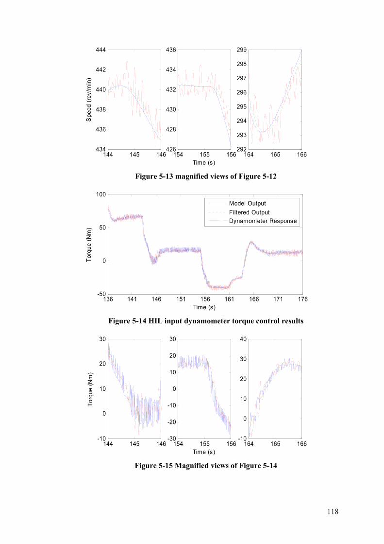
Spe

ed (

rev/

min

) T

orqu

e (N

m)

444 436 299

298 442 434

297

440 432 296

295438 430

294 436 428

293

434 426 292 144 145 146 154 155 156 164 165 166

Time (s)

Figure 5-13 magnified views of Figure 5-12

136 141 146 151 156 161 166 171 176 Time (s)

Figure 5-14 HIL input dynamometer torque control results

30 30 40

20 3020

1020

10 0

10-10

00-20

-10 -30 -10 144 145 146 154 155 156 164 165 166

Time (s)

Figure 5-15 Magnified views of Figure 5-14

-50

0

50

100

Tor

que

(Nm

)

Model Output

Filtered Output Dynamometer Response

118

As discussed in Section 4.3.2, additional PID controllers may further improve the

compensation results. Therefore, further tests were carried out with additional PID

controllers for both input and output dynamometers. The control errors are derived

from the dynamometer responses and the real time model outputs as the inputs of the

PID controllers. The same PID parameters are used here as in Section 4.3.2. The

proportional, integral and derivative gains are 0.08, 0.4 and 0 for the output

dynamometer speed control and 0.03, 0.3 and 0 for the input dynamometer torque

control.

The output dynamometer speed control results are shown in Figure 5-16, and three

magnified views are shown in Figure 5-17, while the input dynamometer torque

control results are shown in Figure 5-18 and three magnified views are shown in

Figure 5-19. Compared with the magnified views shown in Figures 5-13 and 5-15,

phase responses are further improved for both speed and torque control, e.g. between

164 s and 166 s for the speed control and between 154 s and 156 s for the torque

control. There is no obvious change in the speed amplitude with additional PID

controller. The torque amplitude is sometimes slightly worse than before, e.g.

between 164 s and 166 s shown in Figures 5-15 and 5-19. The control errors are

made within +/- 3 rev/min for the output dynamometer speed control and +/- 5 Nm

for the input dynamometer torque control. Therefore, the use of additional PID

controllers is reasonable in this case. Except for the noises in the measured speed and

torque signals, the input and output dynamometer responses are controlled to follow

the simulation results of the real time engine and vehicle models.

Time (s)

Figure 5-16 HIL output dynamometer speed control with additional PID

136 141 146 151 156 161 166 171 176 250

300

350

400

450

Spe

ed (

rev/

min

)

Model Output

Filtered Output Dynamometer Response

119

442 435 302

300 440

298 438

430 296

436 294

434 292

432 425 290 144 145 146 154 155 156 164 165 166

Time (s)

Figure 5-17 Magnified views of Figure 5-16

Spe

ed (

rev/

min

)

-50

0

50

100

Tor

que

(Nm

)

Model Output

Filtered Output

Dynamometer Response

140 145 150 155 160 165 170 175 Time (s)

Figure 5-18 HIL input dynamometer torque control with additional PID

40 30 30

2030 20

Tor

que

(Nm

) 1020 10

0

10 0 -10

0 -10-20

-10 -30 -20 144 145 146 154 155 156 164 165 166

Time (s)

Figure 5-19 Magnified views of Figure 5-18

120

Chapter 6 Conclusions

In this chapter conclusion is drawn for the programme of research, and potential

future work is also described.

6.1 Conclusions

In this programme of research, a hardware in the loop test facility has been

developed for automotive powertrains, with a particular interest in testing CVTs.

Two electric motors were utilized to substitute the real engine and vehicle and test

CVTs installed in between. In order to provide the same testing environment as in a

real engine and vehicle, real-time engine and vehicle models can be employed to

demand virtual driving torque and vehicle speed from the dynamometers. In this

thesis, digital controllers were designed for the input and output dynamometers to

accurately track these demands

A feedforward control scheme based on the input-output inverse technique was

employed to achieve a perfect tracking. First of all, linearized system models for the

original plant were identified. Since there were unstable zeros in the identified

models, direct inversion was not possible. Among the reviewed literature, ZPETC

was used as the initial design of the feedforward controller to achieve zero phase

shift for all frequencies. Then the design of the feedforward controller mainly

focused on four aspects: (a) the further improvement of gain characteristics, (b) the

optimal design, (c) the causality and (d) the enhancement of robustness to parameter

variations.

For the first two aspects, a digital preview filter (DPF) was designed to approximate

the inverse of the unstable zeros. The gain characteristics were improved by adding

more zeros into the controllers. A penalty function was formulated within the desired

frequency range and minimized by Lagrange method.

121

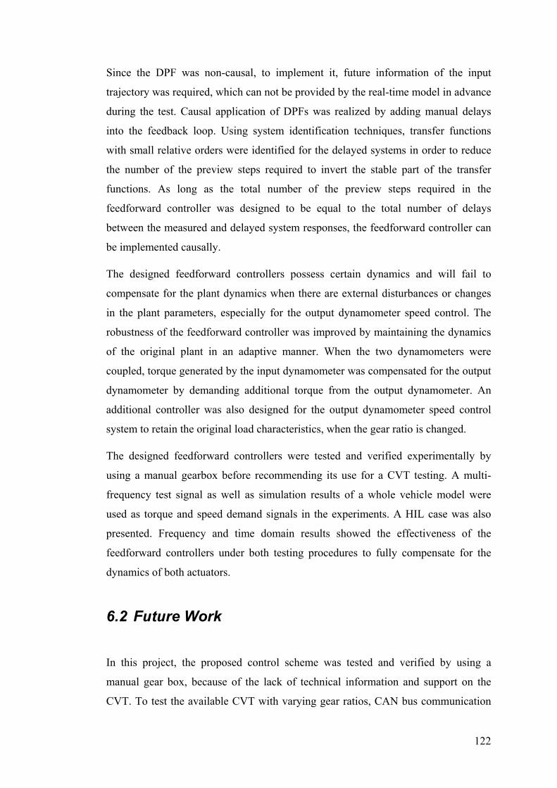
Since the DPF was non-causal, to implement it, future information of the input

trajectory was required, which can not be provided by the real-time model in advance

during the test. Causal application of DPFs was realized by adding manual delays

into the feedback loop. Using system identification techniques, transfer functions

with small relative orders were identified for the delayed systems in order to reduce

the number of the preview steps required to invert the stable part of the transfer

functions. As long as the total number of the preview steps required in the

feedforward controller was designed to be equal to the total number of delays

between the measured and delayed system responses, the feedforward controller can

be implemented causally.

The designed feedforward controllers possess certain dynamics and will fail to

compensate for the plant dynamics when there are external disturbances or changes

in the plant parameters, especially for the output dynamometer speed control. The

robustness of the feedforward controller was improved by maintaining the dynamics

of the original plant in an adaptive manner. When the two dynamometers were

coupled, torque generated by the input dynamometer was compensated for the output

dynamometer by demanding additional torque from the output dynamometer. An

additional controller was also designed for the output dynamometer speed control

system to retain the original load characteristics, when the gear ratio is changed.

The designed feedforward controllers were tested and verified experimentally by

using a manual gearbox before recommending its use for a CVT testing. A multi­

frequency test signal as well as simulation results of a whole vehicle model were

used as torque and speed demand signals in the experiments. A HIL case was also

presented. Frequency and time domain results showed the effectiveness of the

feedforward controllers under both testing procedures to fully compensate for the

dynamics of both actuators.

6.2 Future Work

In this project, the proposed control scheme was tested and verified by using a

manual gear box, because of the lack of technical information and support on the

CVT. To test the available CVT with varying gear ratios, CAN bus communication

122

needs to be set up between the CVT ECU and the engine ECU, where the CVT can

gather information about the driving condition and determine the optimal gear ratio.

To set up the communication, real-time engine and ECU models with a proper level

of simulation complexity are required. The models need to provide all the required

interfaces to the CVT ECU. Alternatively, the engine ECU can exist in the hardware

form and interface with real-time engine model and the CVT ECU.

The design of the feedforward controller in this project was based on the trial of

adding different delays to the feedback loop and estimating the transfer functions

with low relative orders. Generally speaking, the feedforward controller would offer

better performance with more future values, which means more delays needed to be

added to the feedback loop to make the feedforward controller causal. But adding

more delay may make the feedback control unstable, and also may not give good fit

when estimating the transfer function. Hence, future work is required to find an

optimal number of manual delays added to the feedback loop and optimal orders for

the numerator and denominator of the estimated transfer functions, to offer the best

fit and at the same time the best compensation.

123

References

[1] L.Fel, "Development of the Ball Toroidal Continuously Variable Transmission," SAE Technical Paper 981479, 1998.

[2] Y.Ono, M.Goto, R.Yamashita, Y.Hasuda, and S.Yasuhara, "The Durability and Reliability of Variators for a Dual-cavity Full-toroidal CVT," SAE Technical Paper 2000-01-0826, 2000.

[3] H.Aitzetmüller, "Steyr S-Matic~The future CVT system," SAE Technical Paper 2000-05-0129, 2000.

[4] P.Kanphet, P.Jirawattana, and B.Direcksataporn, "Optimal Operation and Control of a Hydrostatic CVT Powertrain," SAE Technical Paper 2005-01-1467, 2005.

[5] C.J.Brace, M.Deacon, N.D.Vaughan, R.W.Horrocks, and C.R.Burrows, "An Operation Point Optimizer for the Design and Calibration of an Integrated DieselContinuously variable Transmission Powertrain," Proceedings of the Institution of Mechanical Engineers. Part D, Journal of Automobile Engineering, vol. 213 1999.

[6] K.Osamura, H.Itoyama, and H.Iwano, "Study of an Integrated Diesel Engine-CVT Control Algorithm for Improving Drivability and Exhaust Emission Performance," SAE Technical Paper 2001-01-3452, 2001.

[7] S.Sakaguchi, E.Kimura, and K.Yamamoto, "Development of an Engine-CVT Integrated Control System," SAE Technical Paper 1999-01-0754, 1999.

[8] T.Kim and H.Kim, "Performance of Integrated Engine-CVT Control Considering Powertrain Loss and CVT Response Lag," Proceedings of the Institution of Mechanical Engineers. Part D, Journal of Automobile Engineering, vol. 216 2002.

[9] K.Osamura, H.Itoyama, and H.Iwano, "Improvement of Drive Torque Response by Applying an Integrated Control Algorithm for a Diesel Engine and CVT," JSAE Review 22, 2001.

[10] M.Yasuoka, M.Uchida, S.Katakura, and T.Yoshino, "An Integrated Control Algorithm for an SI Engine and a CVT," SAE Technical Paper 1999-01-0752, 1999.

124

[11] S.Takahashi, "Fundamental Study of Low Fuel Consumption Control Scheme Based on Combination of Direct Fuel Injection Engine and Continuously Variable Transmission," 1998.

[12] S.Liu and B.Paden, "A Survey of Today's CVT Controls," 1997.

[13] M.A.Kluger and D.M.Long, "An Overview of Current Automatic, Manual and Continuously Variable Transmission Efficiencies and Their Projected Future Improvements," SAE Technical Paper 1999-01-1259, 1999.

[14] F.Sluis, T.Dongen, G.Spijk, A.velde, and A.Heeswijk, "Efficiency Optimization of the Pushbelt CVT," SAE Technical Paper 2007-01-1457, 2007.

[15] R.Kataoka, K.Okubo, T.Fujii, and S.Kanehara, "A Study on a Metal Pushing V-belt type CVT - A Novel Approach to Characterize the Friction Between Blocks and a Pulley, and Shifting Mechanisms," SAE Technical Paper 2002-01-0697, 2002.

[16] H.Nishizawa, H.Yamaguchi, H.Suzuki, M.Osawa, K.Iwatuki, and Y.Oshiumi, "Friction Characteristics Analysis for Clamping Force Setup in Metal V-Belt Type CVT," SAE Technical Paper 2005-01-1462, 2005.

[17] H.Yamaguchi, H.Nishizawa, H.Suzuki, K.Iwatuki, and K.Hoshiya, "Development of Belt Saturation Detection Method for V-Belt Type CVT," SAE Technical Paper 2004-01-0479, 2004.

[18] H.Lee and H.Kim, "Analysis of Primary and Secondary Thrusts for A Metal Belt CVT Part 1: New Formula for Speed Ratio-Torque-Thrust Relationship Considering and Tension and Block Compression," SAE Technical Paper 2000-01-0841, 2000.

[19] S.Akehurst, D.A.Parker, and N.D.Vaughan, "Potential for Fuel Economy Improvements by Reducing Frictional Losses in a Pushing Metal V-Belt CVT," SAE Technical Paper 2004-01-0481, 2004.

[20] M.Drogen and M.Laan, "Determination of Variator Robustness Under Macro Slip Conditions for a Push Belt CVT," SAE Technical Paper 2004-01-0480, 2004.

[21] T.Saito and A.D.Lewis, "Development of a Simulation Technique for CVT Metal Pushing V-Belt with Feedback Control," SAE Technical Paper 2004-01-1326, 2004.

[22] A.Ohashi, Y.Sato, K.Kajikawa, S.Sakuma, J.Urano, M.Yamaguchi, and A.Shibahara, "Development of High-efficiency CVT for Luxury Compact Vehicle," SAE Technical Paper 2005-01-1019, 2005.

[23] H.Takahara, H.Yasue, R.Habuchi, T.Ishihara, S.Tsuzuki, and J.Maeda, "Continuously Variable Transmission Control System for Toyota Intelligent Idling Stop System," SAE Technical Paper 2004-01-1635, 2004.

125

[24] T.H.Bradley, B.R.Huff, and A.A.Frank, "Energy Consumption Test Methods and Results for Servo-Pump Continuously Variable Transmission Control System," SAE Technical Paper 2005-01-3782, 2005.

[25] E.A.Solik, A.A.Frank, and P.A.Erickson, "Design Improvements on a Vee Belt CVT and Application to a New In-line CVT Concept," SAE Technical Paper 2005-01-3459, 2005.

[26] J.Jantos, "Control of the Transmission Ratio Derivative in Passenger Car Powertrain with CVT," SAE Technical Paper 2001-01-1159, 2001.

[27] A.F.A.Serrarens, S.Shen, and F.E.Veldpaus, "Control of a Flywheel Assisted Driveline with Continuously Variable Transmission," Journal of Dynamic System, Measurement, and Control, 2003.

[28] J.E.Mahoney, J.M.Maguire, and S.Bai, "Ratio Changing the Continuously Variable Transmission," SAE Technical Paper 2004-01-1634, 2004.

[29] A.F.A.Serrarens and F.E.Veldpaus, "Powertrain Control of a Flywheel Assisted Driveline with CVT," Proceedings of the International Congress on Continuously Variable Transmissions, Eindhoven (1999), 1999.

[30] V.Wicke, C.J.Brace, M.Deacon, and N.D.Vaughan, "Preliminary Results from Driveability Investigations of Vehicles with Continuously Variable Transmission," Int. Congress on Continuously Variable Power Transmission CVT'99, 1999.

[31] D.Patel, J.Ely, and M.Overson, "CVT Drive Research Study," SAE Technical Paper 2005-01-1459, 2005.

[32] D.F.Pick, D.Yuan D.Wang, R.W.Proctor, and D.Patel, "Dead Pedal and the Perception of Performance of a Continuously Variable Transmission," SAE Technical Paper 2005-01-1596, 2005.

[33] V.Wicke, C.J.Brace, and N.D.Vaughan, "The Potential for Simulation of Driveability of CVT Vehicles," SAE Technical Paper 2000-01-0830, 2000.

[34] K.Abo, M.Kobayashi, and M.Kurosawa, "Development of a Metal Belt-Drive CVT Incorporating a Torque Converter for Use with 2-Liter Class Engines," SAE Technical Paper 980823, 1998.

[35] M.S.Castiglione, G.Stecklein, R.Senseney, and D.Stark, "Development of Transmission Hardware-in-the-loop Test System," SAE Technical Paper 2003-01-1027, 2003.

[36] A.Wagener, H.Kabza, C.Koerner, and P.Seger, "Model-based Drivetrain Development and Rapid Prototyping For a Hybrid Electric Car," Automotive and Transportation Technology Congress and Exhibition, 2001.

[37] M.Adenmark, M.Deter, and T.Schulte, "Testing Networked ECUs in a HIL Based Integration Lab," SAE Technical Paper 2006-01-3495, 2006.

126

[38] A.Wanpal, M.G.Babu, and N.Kankariya, "ECU Testing and Verification Using Hardware-in-the-Loop," SAE Technical Paper 2006-01-1444, 2006.

[39] M.B.Ganesh, "Hardware in the Loop Simulation (HIL) for Vehicle Electronics Systems Testing and Validation," SAE Technical Paper 2005-26-304, 2005.

[40] J.Gehring and H.Schutte, "A Hardware-in-the-Loop Test Bench for Validation of Complex ECU Networks," SAE Technical Paper 2002-01-0801, 2002.

[41] S.Kohl and D.Jegminat, "How to Do Hardware-in-the-Loop Simulation Right," SAE Technical Paper 2005-01-1657, 2005.

[42] P.J.Gawthrop, D.W.Virden, S.A.Neild, and D.J.Wagg, "Emulator-based Control for Actuator-based Hardware-in-the-Loop Testing," Control Engineering Practice, vol. 16, no. 8, pp. 897-908, 2008.

[43] M.Velardocchia and A.Sorniotti, "Hardware-in-the-Loop to Evaluate Active Braking Systems Performance," SAE Technical Paper 2005-01-1580, 2005.

[44] W.E.Misselhorn, N.J.Theron, and P.S.Els, "Investigation of Hardware-in-the-Loop for Use in Suspension Development," Vehicle System Dynamics, vol. 44, no. 1, pp. 65-81, 2006.

[45] A.Blakeborough, M.S.Williams, A.P.Darby, and D.M.Williams, "The Development of Real-Time Substructure Testing," Philosophical Transactions: Mathematical, Physical and Engineering Sciences, vol. 359, no. 1786, pp. 1869-1891, 2001.

[46] A.P.Darby, M.S.Williams, and A.Blakeborough, "Stability and Delay Compensation for Real-Time Substructure Testing," Journal of Engineering Mechanics, vol. 128, no. 12, pp. 1276-1284, 2002.

[47] M.Tomizuka, "Zero Phase Error Tracking Algorithm for Digital Control," Journal of Dynamic Systems, Measurement and Control, vol. 109, no. 1, pp. 65-68, 1987.

[48] J.A.Butterworth, L.Y.Pao, and D.Y.Abramovitch, "The Effect of Nonminimum-phase Zero Locations on the Performance of Feedforward Model-inverse Control Techniques in Discrete-time Systems," 2008 American Control Conference, 2008.

[49] B.Haack and M.Tomizuka, "The Effect of Adding Zeros to Feedforward Controllers," Journal of Dynamic Systems, Measurement and Control, vol. 113, no. 1, pp. 6-10, 1991.

[50] C.Menq and J.Chen, "Precision Tracking Control of Discrete Time Nonminimum-Phase Systems," Journal of Dynamic Systems, Measurement and Control, vol. 115, no. 2A, pp. 238-245, 1993.

127

[51] J.Z.Xia and C.Menq, "Precision Tracking Control of Non-minimum Phase Systems with Zero Phase Error," International Journal of Control, vol. 61, no. 4, pp. 791-807, 1995.

[52] S.Yeh and P.Hsu, "An Optimal and Adaptive Design of the Feedforward Motion Controller," IEEE/ASME Transactions on Mechatronics, vol. 4, no. 4, pp. 428-439, 1999.

[53] E.Gross, M.Tomizuka, and W.Messner, "Cancellation of Discrete Time Unstable Zeros by Feedforward Control," Journal of Dynamic Systems, Measurement and Control, vol. 116, no. 1, pp. 33-38, 1994.

[54] E.Gross and M.Tomizuka, "Experimental Flexible Beam Tip Tracking Control with a Truncated Series Approximation to Uncancelable Inverse Dynamics," IEEE Transactions on Control Systems Technology, vol. 2, no. 4, pp. 382-391, 1994.

[55] B.Choi and C.Choi, "A Feedforward Controller by Modified Series Approximation," IEEE/ASME Transactions on Mechatronics, vol. 3, no. 3, pp. 249-251, 1998.

[56] D.Torfs, J.Swevers, and J.De Schutter, "Quasi-perfect Tracking Control of Non-minimal Phase Systems," Proceedings of the 30th Conference on Decision and Control, 1991.

[57] D.Torfs, J.De Schutter, and J.Swevers, "Extended Bandwidth Zero Phase Error Tracking Control of Nonminimal Phase Systems," Journal of Dynamic Systems, Measurement and Control, vol. 114, no. 3, pp. 347-351, 1992.

[58] M.M.Mustafa, "Trajectory-adaptive Digital Tracking Controllers for Non-minimum Phase Systems without Factorisation of Zeros," IEE Proceedings: Control Theory and Applications, vol. 149, no. 2, pp. 157-162, 2002.

[59] M.Yamada, Y.Funahashi, and S.Fujiwara, "Zero Phase Error Tracking System with Arbitrarily Specified Gain Characteristics," Journal of Dynamic System, Measurement, and Control, vol. 119, no. 2, pp. 260-264, 1997.

[60] M.Yamada, Y.Funahashi, and Z.Riadh, "Generalized Optimal Zero Phase Error Tracking Controller Design," Journal of Dynamic Systems, Measurement and Control, vol. 121, no. 2, pp. 165-170, 1999.

[61] G.Marro and L.Marconi, "Using the Diophantine Equation in the Design of a Digital Perfect Tracking Compensator," Proceedings of 16th Benelux Meeting on Systems and Control, 1997.

[62] L.Marconi, G.Marro, and C.Melchiorri, "A Solution Technique for Almost Perfect Tracking of Non-minimum-phase, Discrete-time Linear System," International Journal of Control, vol. 74, no. 5, pp. 496-506, 2001.

[63] T.Tsao and M.Tomizuka, "Adaptive Zero Phase Error Tracking Algorithm for Digital Control," Journal of Dynamic Systems, Measurement and Control, vol. 109, no. 4, pp. 349-354, 1987.

128

[64] B.Widrow and M.Bilello, "Adaptive Inverse Control," Proceedings of the 1993 IEEE International Symposium on Intelligent Control, 1993.

[65] Y.Gu and M.Tomizuka, "Multi-rate Feedforward Tracking Control for Plants with Nonminimum Phase Discrete Time Models," Proceedings of the American Control Conference, vol. 6, pp. 4290-4294, 1999.

[66] C.R.Burrows and M.N.Sahinkaya, "Frequency-Domain Estimation of Linearized Oil-Film Coefficients," ASME Joint Lubrication Conference, 1981.

[67] M.N.Sahinkaya, M.O.T.Cole, and C.R.Burrows, "On the Use of Schroeder Phased Harmonic Sequences in Multi-Frequency Vibration Control of Flexible Rotor/Magnetic Bearing Systems," 8th International Symposium on Magnetic Bearings, 2002.

[68] M.R.Schroeder, "Synthesis of Low-Peak-Factor Signals and Binary Sequences with Low Autocorrelation," IEEE Transactions on Information Theory, 1969.

[69] T.Tsao, "Optimal Feed-Forward Digital Tracking Controller Design," Journal of Dynamic System, Measurement, and Control, vol. 116, no. 4, pp. 583-592, 1994.

[70] M.M.Mustafa, N.R.Yaacob, and N.A.Nik Mohamed, "Adaptive Zero-Phase Error-Tracking Controller with Advanced Learning," Control and Intelligent Systems, vol. 32, no. 2, pp. 116-125, 2004.

129