cavity basics - cas.web.cern.ch · pdf fileelectromagnetic field experiences a force ... c c c...

Cavity Basics

Erk Jensen

CERN BE‐RF

What is a cavity?

11‐6‐2010 CAS RF Denmark ‐

Cavity Basics 2

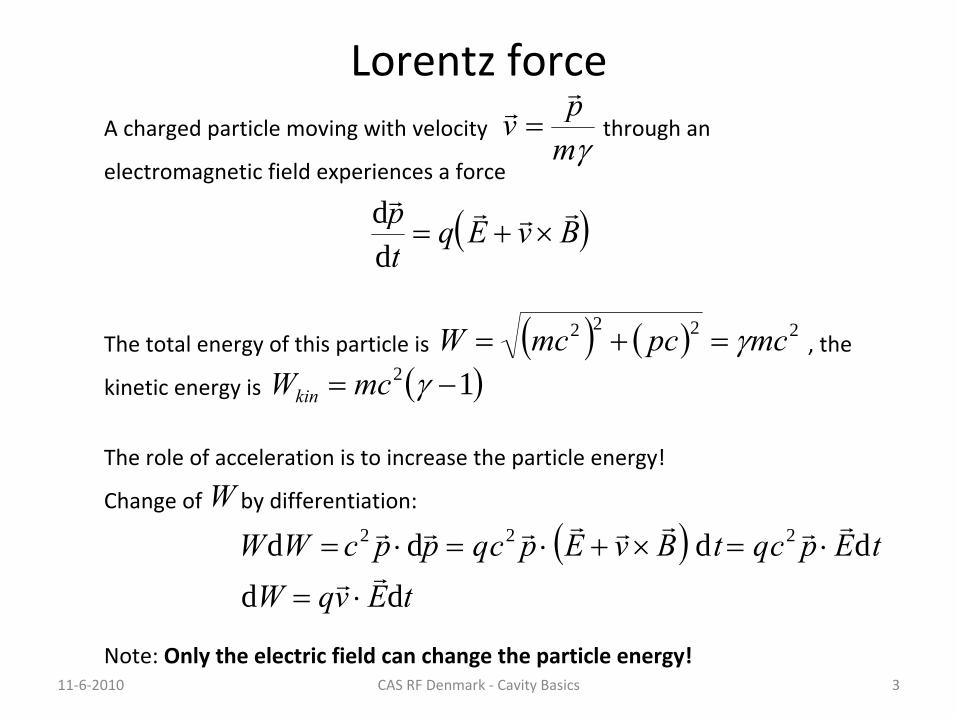
Lorentz forceA charged particle moving with velocity through an

electromagnetic field experiences a force

The total energy of this particle is

, the

kinetic energy is 12 mcWkin

2222 mcpcmcW

mpv

BvEqtp

dd

The role of acceleration is to increase the particle energy!

Change of by differentiation:W tEpcqtBvEpcqppcWW dddd 222

tEvqW dd

Note: Only the electric field can change the particle energy!11‐6‐2010 3CAS RF Denmark ‐

Cavity Basics

Maxwell’s equations

11‐6‐2010 4CAS RF Denmark ‐

Cavity Basics

00

0012

EBt

E

BEtc

B

The electromagnetic fields inside the “hollow place”

obey these equations:

With the curl of the 3rd, the time derivative of the 1st

equation and the

vector identity

EEE

this set of equations can be brought in the form

012

2

2

Etc

E

which is the Laplace equation in 4 dimensions.

With the boundaries of the “solid body”

around it (the cavity walls), there

exist eigensolutions of the cavity at certain frequencies (eigenfrequencies).

Wave vector

: the direction of is the direction of

propagation,the length of is the phase shift per

unit length.behaves like a vector.

Homogeneous plane wave

CAS RF Denmark ‐

Cavity Basics 5

z

x

Ey

φ

11‐6‐2010

rktuB

rktuE

x

y

coscos k

k

k

k

xzc

rk sincos

ck c

ck

2

1

c

z ck

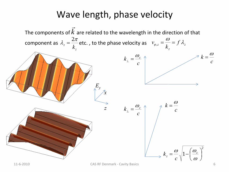
The components of are related to the wavelength in the direction of that

component as etc. , to the phase velocity as

Wave length, phase velocity


Cavity Basics 6

z

xEy

k

ck c c

k

2

1

c

z ck

ck c c

k

zz k

2 z

zz f

kv ,

Superposition of 2 homogeneous plane waves

CAS RF Denmark ‐

Cavity Basics 7

+=

Metallic walls may be inserted where

without perturbing

the fields.

Note the standing wave in x‐direction!

z

xEy

This way one gets a hollow rectangular waveguide

11‐6‐2010

0yE

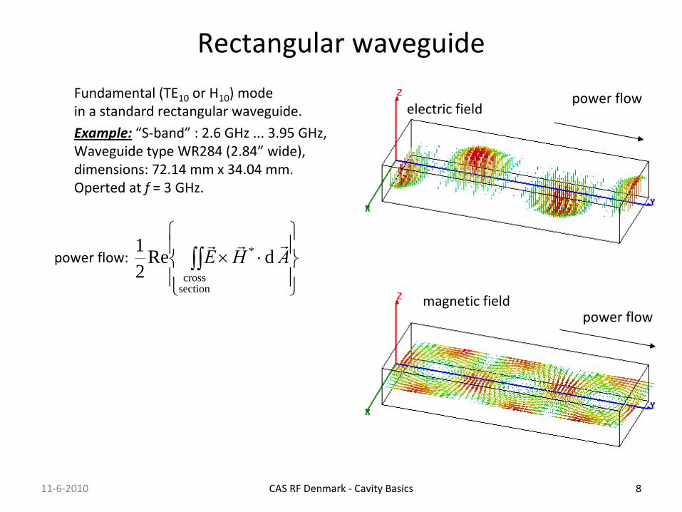
Rectangular waveguide

CAS RF Denmark ‐

Cavity Basics 8

Fundamental (TE10

or H10

) modein a standard rectangular waveguide.Example:

“S‐band”

: 2.6 GHz ... 3.95 GHz,Waveguide type WR284 (2.84”

wide),

dimensions: 72.14 mm x 34.04 mm.Operted at f

= 3 GHz.

electric field

magnetic field

power flow:

power flow

power flow

11‐6‐2010

sectioncross

* dRe21 AHE

Waveguide dispersion


Cavity Basics 9

What happens with different waveguide

dimensions (different width a)?

c

zk

1:

a

= 52 mm,

f/fc

= 1.04

cutoff

2

12

c

gz c

k

ck

acfc 2

f

= 3 GHz

2:a

= 72.14 mm,

f/fc

= 1.44

3:a

= 144.3 mm,

f/fc

= 2.881

2

3

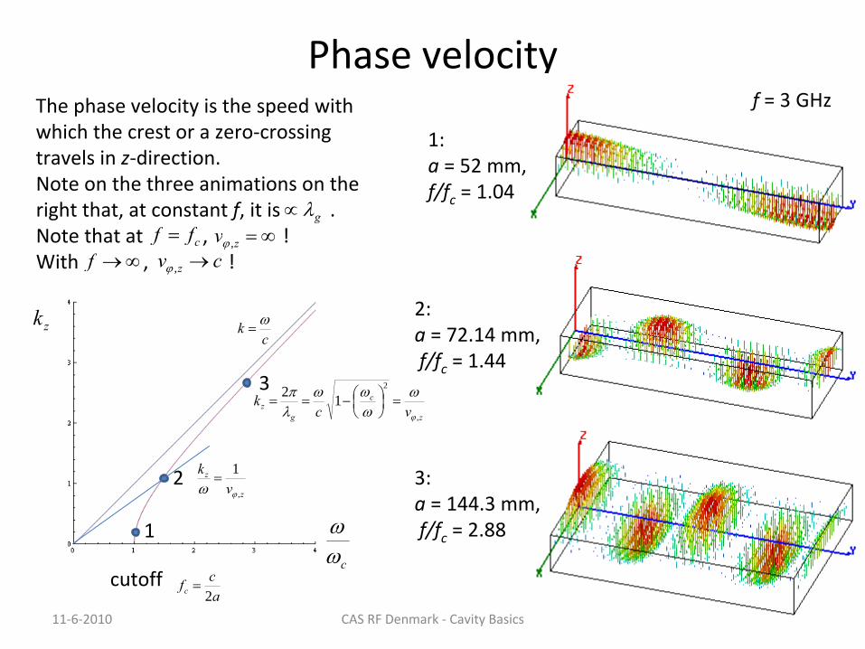
Phase velocity


Cavity Basics 10

The phase velocity is the speed with

which the crest or a zero‐crossing

travels in z‐direction.Note on the three animations on the

right that, at constant f, it is .Note that at , ! With , !

c

zk

cutoff

z

c

gz vc

k,

2

12

ck

acfc 2

gcff zv ,

f

= 3 GHz

z

z

vk

,

1

f cv z ,

1

2

3

1:

a

= 52 mm,

f/fc

= 1.04

2:a

= 72.14 mm,

f/fc

= 1.44

3:a

= 144.3 mm,

f/fc

= 2.88

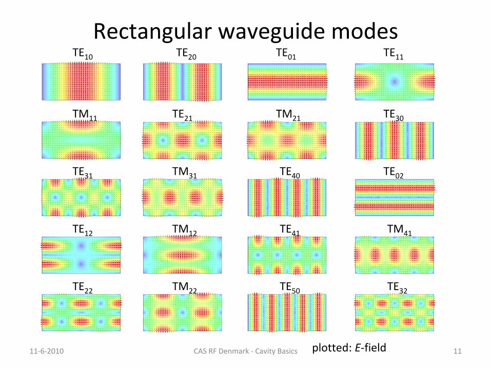
Rectangular waveguide modes


Cavity Basics 11

TE10 TE20 TE01 TE11

TM11 TE21 TM21 TE30

TE31 TM31 TE40 TE02

TE12 TM12 TE41 TM41

TE22 TM22 TE50 TE32

plotted: E‐field

Radial waves


Cavity Basics 12

nkHE nz cos2 nkHE nz cos1 nkJE nz cos

Also radial waves may be interpreted as

superpositions of plane waves.The superposition of an outward and an

inward radial wave can result in the field of a

round hollow waveguide.

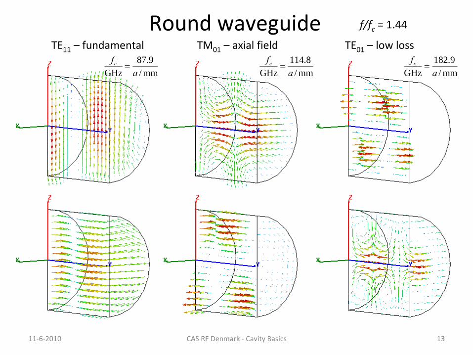
Round waveguide


Cavity Basics 13

f/fc

= 1.44

TE11

–

fundamental

mm/9.87

GHz afc

mm/8.114

GHz afc

mm/9.182

GHz afc

TM01

– axial field TE01

– low loss

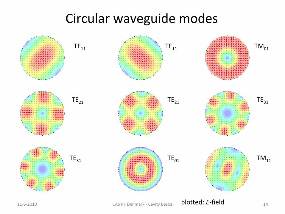
Circular waveguide modes


Cavity Basics 14

TE11 TM01

TE21 TE21

TE11

TE31

TE31 TE01 TM11

plotted: E‐field

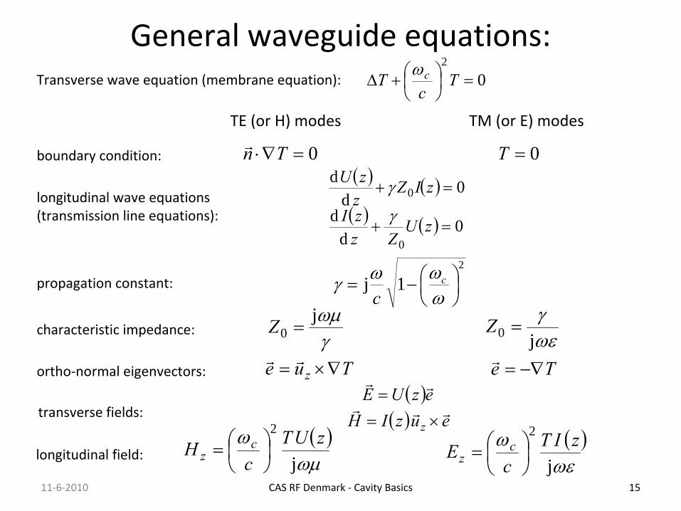
General waveguide equations:

CAS RF Denmark ‐

Cavity Basics 15

02

T

cT c

Transverse wave equation (membrane equation):

TM (or E) modesTE (or H) modes

boundary condition:

longitudinal wave equations

(transmission line equations):

propagation constant:

characteristic impedance:

ortho‐normal eigenvectors:

transverse fields:

longitudinal field:

0 Tn 0T 0

dd

0d

d

0

0

zUZz

zI

zIZzzU

j

0 Z

j0 Z

Tue z Te

euzIH

ezUE

z

j

2 zUTc

H cz

j

2 zITc

E cz

2

1j

c

c

11‐6‐2010

CAS RF Denmark ‐

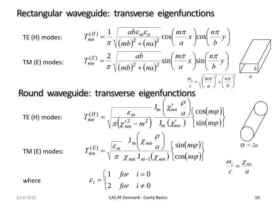
Cavity Basics 16

TM (E) modes:

TE (H) modes:

y

bnx

am

nambabT nmH

mn

coscos1

22)(

y

bnx

am

nambabT E

mn

sinsin2

22)(

0201

iforifor

i

mmaT

mnmmn

mnmmE

mn cossin

J

J

1

)(

mma

mT

mnm

mnm

mn

mHmn sin

cosJ

J

22)(TE (H) modes:

TM (E) modes:

where

Ø = 2a

ab

22

bn

am

cc

acmnc

11‐6‐2010

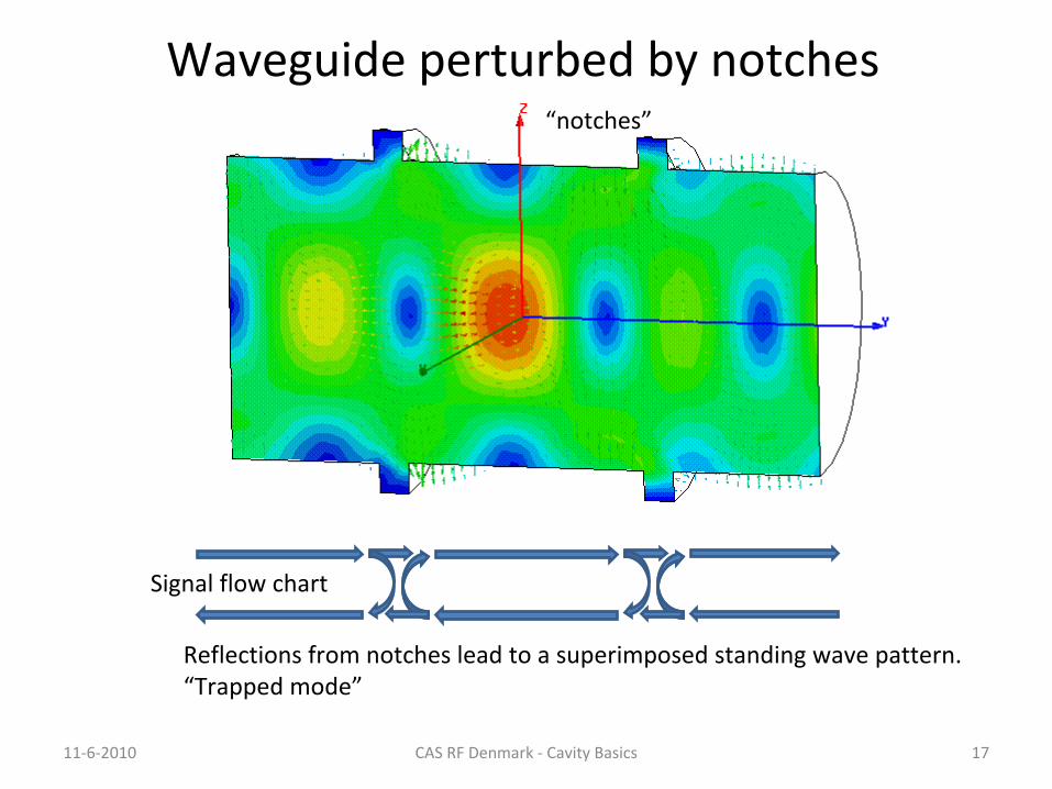
Waveguide perturbed by notches


Cavity Basics 17

“notches”

Reflections from notches lead to a superimposed standing wave pattern.“Trapped mode”

Signal flow chart

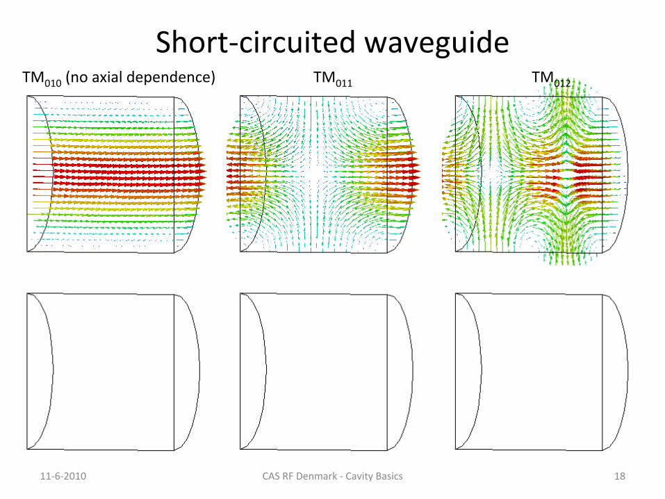
Short‐circuited waveguide


Cavity Basics 18

TM010

(no axial dependence) TM011 TM012

Single WG mode between two shorts


Cavity Basics 19

zke j

zke j

2

1

c

z ck

short

circuit

short

circuit

11

aea zk 2jEigenvalue equation for field amplitude a:

a

Non‐vanishing solutions exist for : mkz 22

Signal flow chart

With , this becomes

222

0 2

mcff c

Simple pillbox


Cavity Basics 20

electric field (purely axial) magnetic field (purely azimuthal)

(only 1/2 shown)

TM010

‐mode

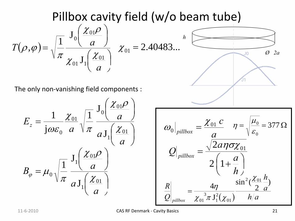
Pillbox cavity field (w/o beam tube)

CAS RF Denmark ‐

Cavity Basics 21

The only non‐vanishing field components :

h

Ø 2a

11‐6‐2010

a

aT01

101

010

J

J1,

...40483.201

aa

aB

aa

aa

Ez

011

011

0

011

010

01

0

J

J1

J

J1

j1

ac

pillbox01

0 377

0

0

ha

aQ pillbox

12

2 01

ahah

QR

pillbox

)2

(sin

J4

012

0121

301

Pillbox with beam pipe

CAS RF Denmark ‐

Cavity Basics 22

electric field magnetic field

(only 1/4 shown)TM010

‐mode

11‐6‐2010

One needs a hole for the beam pipe –

circular waveguide below cutoff

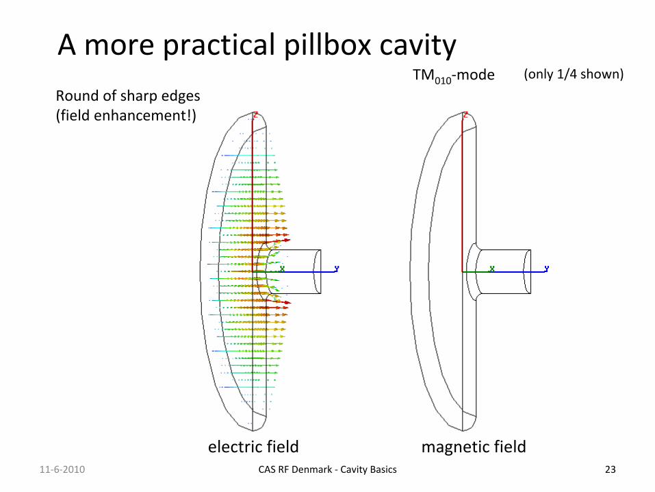
A more practical pillbox cavity

CAS RF Denmark ‐

Cavity Basics 23



‐mode

11‐6‐2010

Round of sharp edges

(field enhancement!)

Stored energy


Cavity Basics 24

The energy stored in the electric field is

cavity

VH d2

2The energy stored in the magnetic field is

1 2 3 4 5 6

1.0

0.5

0.5

1.0

1 2 3 4 5 6

1.0

0.5

0.5

1.0

Since and are 90°

out of phase, the stored energy continuously swaps

from electric energy to magnetic energy. On average, electric and magnetic

energy must be equal.The (imaginary part of the) Poynting vector describes this energy flux.

E

H

cavity

VE d2

2

cavity

VHEW d22

22 In steady state, the total stored energy

is

constant in time.

E

H

EW

MW

Stored energy & Poynting vector


Cavity Basics 25

electric field energy Poynting vector magnetic field energy

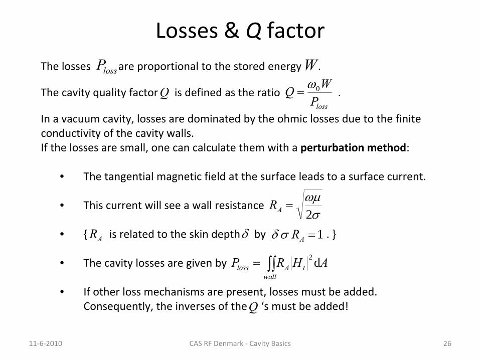
Losses & Q

factor


Cavity Basics 26

The losses are proportional to the stored energy .

In a vacuum cavity, losses are dominated by the ohmic losses due

to the finite

conductivity of the cavity walls.If the losses are small, one can calculate them with a perturbation method:

• The tangential magnetic field at the surface leads to a surface current.

• This current will see a wall resistance

• { is related to the skin depth by

. }

• The cavity losses are given by

• If other loss mechanisms are present, losses must be added.

Consequently, the inverses of the ‘s must be added!

wall

tAloss AHRP d2

2

AR

AR 1AR

WThe cavity quality factor is defined as the ratio

.lossPWQ 0Q

Q

lossP

V

Small boundary perturbation – tuning


Cavity Basics 27

Another application of the perturbation method is to analyse the

sensitivity to

(small) surface geometry perturbations.•This is relevant to understand the effect of fabrication tolerances.•Intentional surface perturbation can be used to tune the cavity.

The basic idea of the perturbation theory is use a known solution (in this case the

unperturbed cavity) and assume that the deviation from it is only small. We just

used this to calculate the losses (assuming would be that without losses).tH

The result of this calculation leads to a convenient expression for the detuning:

V

V

VEH

VEH

d

d2

02

0

20

20

0

0

V

ΔV

0unperturbed

perturbed

“Slater‐theorem”

I define . The exponential factor accounts for the

variation of the field while particles with velocity are

traversing the gap

(see next page).

With this definition, is generally complex – this becomes important

with more than one gap. For the time being we are only interested in

.

Acceleration voltage & R‐upon‐Q


Cavity Basics 28

The proportionality constant defines the quantity called R‐upon‐Q:

The square of the acceleration voltage is proportional to the stored energy . W

WV

QR acc

0

2

2

zeEVz

czacc d

j

Attention, different definitions are used!

accVaccV

Attention, also here different definitions are used!

c

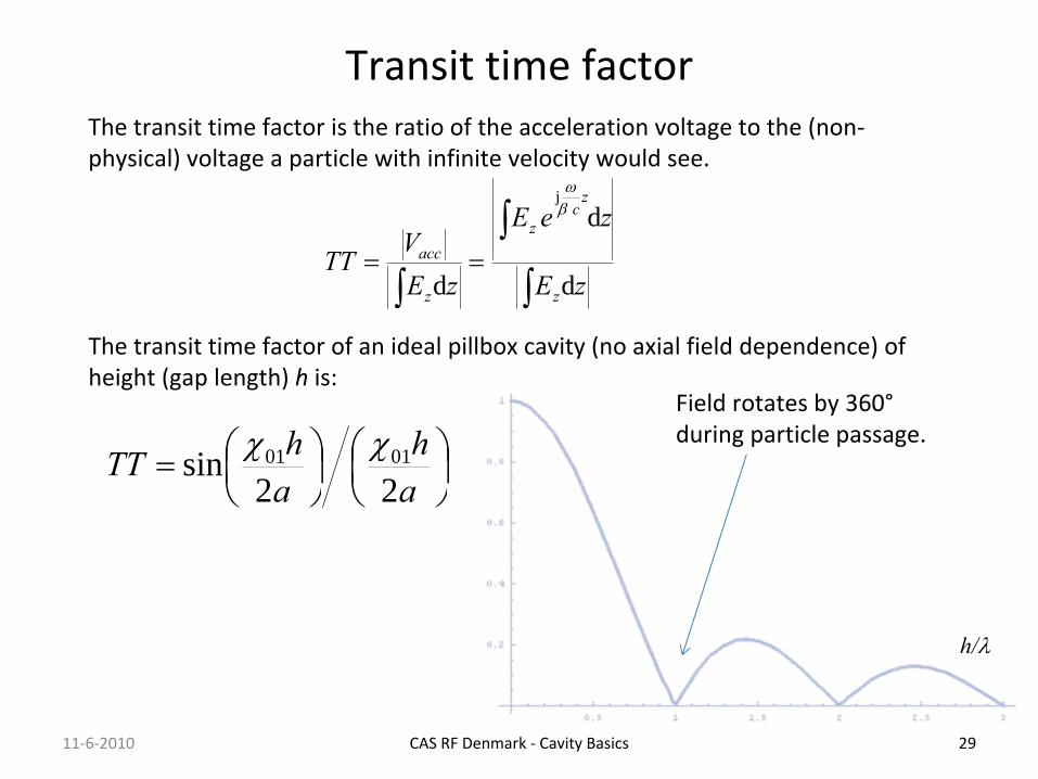
Transit time factor

CAS RF Denmark ‐

Cavity Basics 29

h/

11‐6‐2010

zE

zeE

zEV

TTz

zc

z

z

acc

d

d

d

j

The transit time factor is the ratio of the acceleration voltage

to the (non‐

physical) voltage a particle with infinite velocity would see.

The transit time factor of an ideal pillbox cavity (no axial field dependence) of

height (gap length) h

is:

ah

ahTT

22sin 0101

Field rotates by 360°

during particle passage.

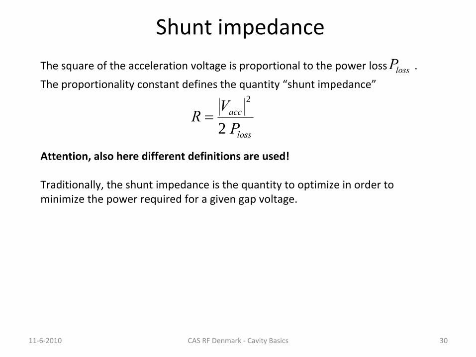
Shunt impedance


Cavity Basics 30

The proportionality constant defines the quantity “shunt impedance”

The square of the acceleration voltage is proportional to the power loss .

Attention, also here different definitions are used!

lossP

loss

acc

PV

R2

2

Traditionally, the shunt impedance is the quantity to optimize in order to

minimize the power required for a given gap voltage.

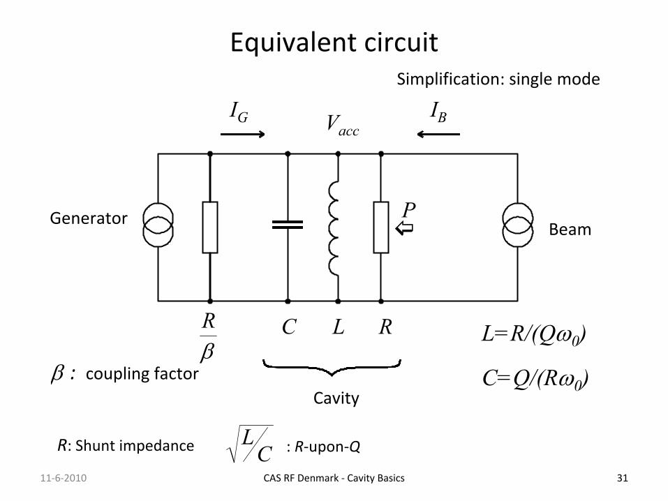
Equivalent circuit

CAS RF Denmark ‐

Cavity Basics 31

R

Cavity

Generator

IG

P

C=Q/(R0

)

Vacc

Beam

IB

L=R/(Q0

)LC

: coupling factor

R: Shunt impedance : R‐upon‐Q

Simplification: single mode

11‐6‐2010

R

CL

Resonance

CAS RF Denmark ‐

Cavity Basics 3211‐6‐2010

Reentrant cavity

CAS RF Denmark ‐

Cavity Basics 33

Example: KEK photon factory 500 MHz

‐

R

probably as good as it gets

‐

this cavity

optimizedpillbox

R/Q:

111 Ω

107.5 Ω

Q:

44270

41630

R:

4.9 MΩ

4.47 MΩ

Nose cones increase transit time factor, round outer shape minimizes losses.

nose cone

11‐6‐2010

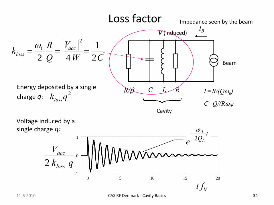
Loss factor

CAS RF Denmark ‐

Cavity Basics 34

0 5 10 15 20

t f0

-1

0

1

qkV

loss

acc

2

Voltage induced by a

single charge

q:t

QLe 20

RR/

Cavity

Beam

C=Q/(R0

)

V

(induced)IB

L=R/(Q0

)LCEnergy deposited by a single

charge q:

Impedance seen by the beam

11‐6‐2010

CWV

QRk acc

loss 21

42

20

2qkloss

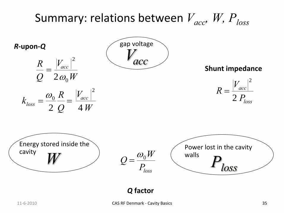
Summary: relations between Vacc

, W, Ploss

CAS RF Denmark ‐

Cavity Basics 35

Energy stored inside the

cavity

Power lost in the cavity

walls

gap voltage

11‐6‐2010

loss

acc

PV

R2

2

WV

QRk acc

loss 42

20

WV

QR acc

0

2

2

lossPWQ 0

R‐upon‐Q

Shunt impedance

Q

factor

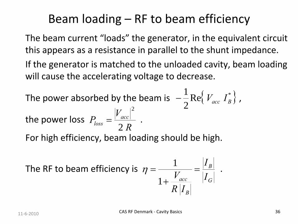
Beam loading – RF to beam efficiencyThe beam current “loads”

the generator, in the equivalent circuit

this appears as a resistance in parallel to the shunt impedance.

If the generator is matched to the unloaded cavity, beam loading

will cause the accelerating voltage to decrease.

The power absorbed by the beam is ,

the power loss .

For high efficiency, beam loading should be high.

The RF to beam efficiency is

.

CAS RF Denmark ‐

Cavity Basics 3611‐6‐2010

*Re21

Bacc IV

RV

P accloss 2

2

G

B

B

acc II

IRV

1

1

Characterizing cavities• Resonance frequency

• Transit time factor

field varies while particle is traversing the gap

• Shunt impedance

gap voltage – power relation

• Q

factor

• R/Qindependent of losses – only geometry!

• loss factor

CAS RF Denmark ‐

Cavity Basics 37

lossacc PRV 22

lossPQW 0

CL

WV

QR acc

0

2

2

CL

10

WV

QRk acc

loss 42

20

Linac definition

lossacc PRV 2

WV

QR acc

0

2

WV

QRk acc

loss 44

20

Circuit definition

zE

zeE

z

zc

z

d

dj

11‐6‐2010

Higher order modes

CAS RF Denmark ‐

Cavity Basics 38

IB

R3

, Q3

,3R2

, Q2

,2R1

, Q1

,1

......

external dampers

n1 n3n2

11‐6‐2010

Higher order modes (measured spectrum)

CAS RF Denmark ‐

Cavity Basics 39

without dampers

with dampers

11‐6‐2010

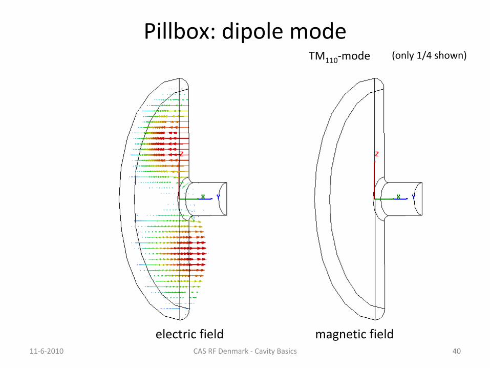
Pillbox: dipole mode


Cavity Basics 40



‐mode

CERN/PS 80 MHz cavity (for LHC)

CAS RF Denmark ‐

Cavity Basics 41

inductive (loop) coupling,

low self‐inductance

11‐6‐2010

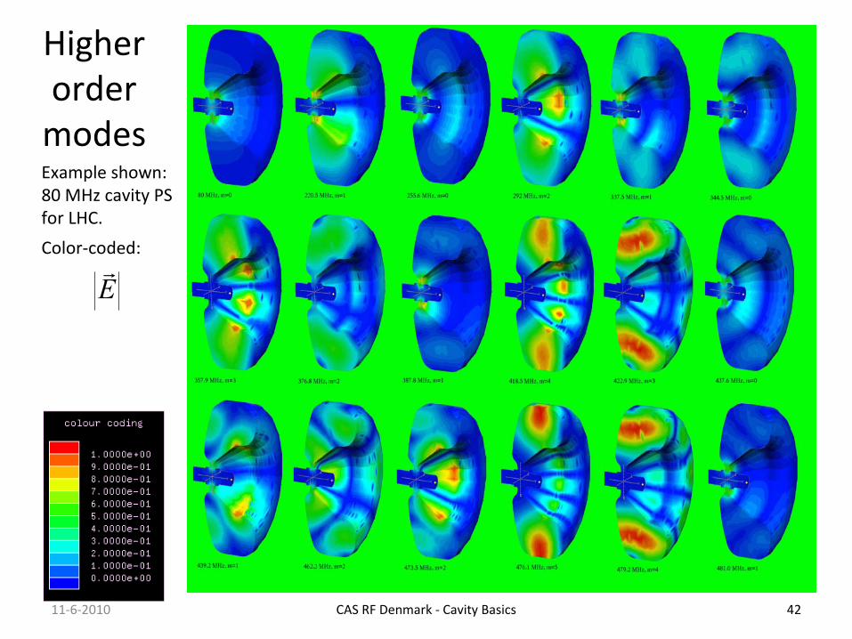
Higher order modes

CAS RF Denmark ‐

Cavity Basics 42

Example shown:80 MHz cavity PS

for LHC.

Color‐coded:

E

11‐6‐2010

What do you gain with many gaps?

CAS RF Denmark ‐

Cavity Basics 43

PnRnPRnVacc 22

•

The R/Q

of a single gap cavity is limited to some 100 Ω.

Now consider to distribute the available power to n

identical

cavities: each will receive P/n, thus produce an accelerating

voltage of .

The total accelerating voltage thus increased, equivalent to a

total equivalent shunt impedance of .

nPR2

nR

1 2 3 n

P/n P/nP/n P/n

11‐6‐2010

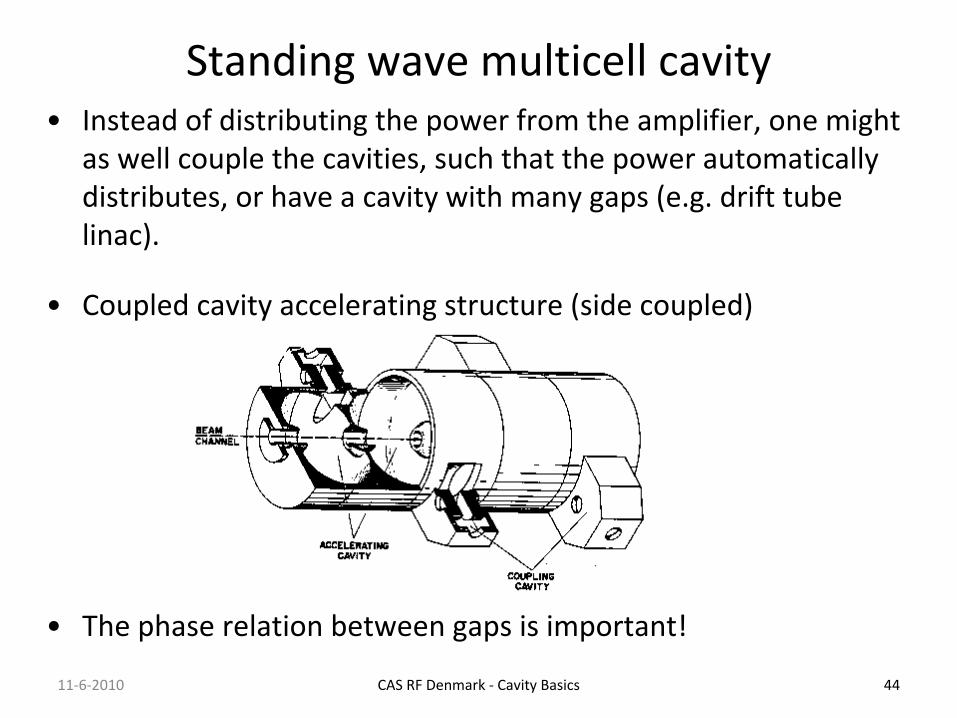
Standing wave multicell cavity

CAS RF Denmark ‐

Cavity Basics 44

•

Instead of distributing the power from the amplifier, one might

as well couple the cavities, such that the power automatically

distributes, or have a cavity with many gaps (e.g. drift tube

linac).

•

Coupled cavity accelerating structure (side coupled)

•

The phase relation between gaps is important!

11‐6‐2010

Brillouin diagram Travelling wave

structure

CAS RF Denmark ‐

Cavity Basics 45

synchronous

2

L/c

speed of light line, /c

L

11‐6‐2010

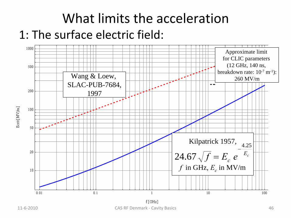
What limits the acceleration1: The surface electric field:


Cavity Basics 46

Kilpatrick 1957,

f

in GHz, Ec

in MV/m

cEc eEf

25.4

67.24

Wang & Loew, SLAC-PUB-7684,

1997

Approximate limit for CLIC parameters

(12 GHz, 140 ns, breakdown rate: 10-7 m-1):

260 MV/m

What limits the acceleration


Cavity Basics 47

2: The surface magnetic fieldThe surface magnetic field leads to a surface current.

For superconducting cavities, it must stay below a threshold value.

For normal conducting cavities, it will lead to local heating, which in turn

can lead to mechanical stress and deformation; with pulsed RF, this can

lead to fatigue stress issues. In the presence of an electric field, the heated

surface can have an effect on the breakdown.

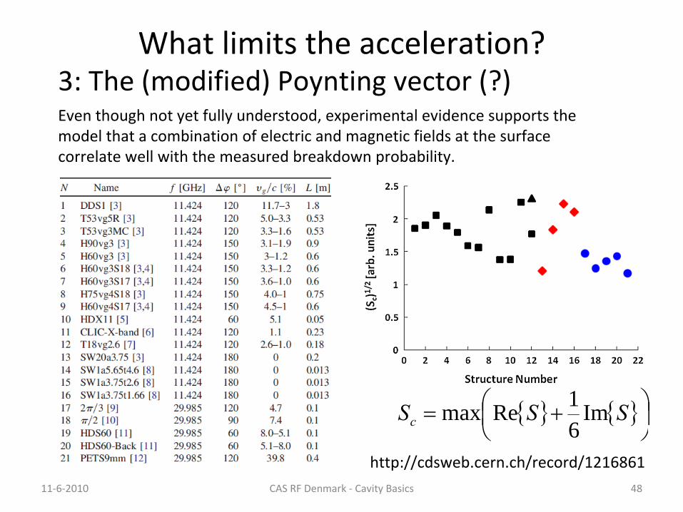
What limits the acceleration?


Cavity Basics 48

3: The (modified) Poynting vector (?)Even though not yet fully understood, experimental evidence supports the

model that a combination of electric and magnetic fields at the surface

correlate well with the measured breakdown probability.

SSSc Im

61Remax

http://cdsweb.cern.ch/record/1216861

Cavity basics –

Summary• The EM fields inside a hollow cavity are superpositions

of

homogeneous plane waves.

• When operating near an eigenfrequency, one can profit from

a resonance phenomenon (with high Q).

• R‐upon‐Q, Shunt impedance and Q

factor were are useful

parameters, which can also be understood in an equivalent

circuit.

• The perturbation method allows to estimate losses and

sensitivity to tolerances.

• Many gaps can increase the effective impedance.


Cavity Basics 49

cavity basics - cas.web.cern.ch · pdf fileelectromagnetic field experiences a force ... c c c...

Documents