ccem.rf-s1.cl (gtrf/02-03) rf power measurements with 2.4

CCEM.RF-S1.CL (GTRF/02-03)

RF Power Measurements with 2.4 mm Connectors

Final Report

Thomas P. CrowleyNational Institute of Standards and Technology

Electromagnetics Division, MC 818.01325 Broadway

Boulder, CO 80305USA

[email protected]

October 12, 2005

Final Report CCEM.RF-S1.CL GTRF/02-03

1

1. IntroductionA comparison of RF power measurements at 8 frequencies was performed on two traveling

standards at 9 national metrology laboratories. The motivation for the comparison was a desire to test measurements at the highest frequencies for which coaxial power calibration services are available. The 2.4 mm coaxial connectors on the standards have single mode operation up to 50 GHz. Although there have been two recent key comparisons for power measurements with coaxial connectors; CCEM.RF-K8.CL and CCEM.RF-K10.CL, there had not been a coaxial power comparison above 26 GHz. Therefore, a supplemental comparison with 2.4 mm connectors and a maximum frequency of 50 GHz was deemed an important test of existing standards.

The comparison was approved by the Working Group on Radio-Frequency Quantities (Groupe de Travail pour les Grandeurs aux Radiofrequences or GTRF) of the Consultative Committee for Electricity and Magnetism (Comite Consultatif d’Electricite et Magnetism or CCEM) in September 2002. Subsequently, BIPM guidelines were adopted stating that supplemental comparisons should be conducted by regional metrology organizations (RMO), and not by the CCEM. However, since the participants of this comparison come from a variety of regions, it was continued under the CCEM.

The participants represent the United States, the United Kingdom, the Netherlands, Switzerland, Canada, South Africa, Australia, Japan, and South Korea. The pilot laboratory was the National Institute of Standards and Technology (NIST) of the United States.

2. Participants and ScheduleThe participants are indicated in Table 1 along with the dates when the standards were at their

laboratory. All participants measured both standards. Three of the participants reported results from frequencies less than or equal to 40 GHz (6 of the 8 frequencies). All other participants measured all frequencies. In addition, 4 laboratories participated in an unofficial comparison at additional frequencies.

The participant list was modified after the comparison was approved to drop one laboratory that had initially expressed interest, but did not join. One other laboratory was added. Several participants were asked to move up their measurement periods as a result of these changes and all agreed. The schedule listed in the protocol in Appendix C reflects some, but not all of these changes. Contact information for several participants changed between the protocol and report stages. Table 1 shows the most recent information.

The comparison was performed in two loops with each participant given two months to complete their measurements and ship the standards to the next participant. An ATA Carnet was used for both loops. The customs documents were not processed properly on leaving the pilot laboratory’s country at the start of the second loop. This resulted in a delay of about two months. The first participant in the loop (CSIR) performed their measurements very quickly which allowed the comparison to stay nearly on schedule.

No damage occurred to the traveling standards during the comparison. Two minor problems occurred with the auxiliary equipment that was circulated. A fuse blew out on the power meter when the switch for the line voltage was not set properly. One of the participants in the first loop noted that the 2.4 mm to Type N adapter used on the calibration output of the power meter had an off-center pin. A different adapter was used on the second loop.

3. Traveling StandardsThe traveling standards consisted of two Agilent 8487A thermocouple power sensors. The device

serial numbers are 3318A03629 and 3318A03815. They will be referred to as device 3629 and device 3815 respectively. A Hewlett Packard (now Agilent) 437B power meter was shipped with the traveling standards and all laboratories performed their measurements with this power meter. The operating frequency range of the sensors is 50 MHz to 50 GHz with a maximum power of 300 mW. They are controlled by the power meter which measures power relative to a reference power of 1 mW at 50 MHz. The sensors and power meter are shown in Figure 1.


2

Contact

JeongHwan [email protected]

Kazuhiro Shimaoka [email protected]

Tieren [email protected]

Erik [email protected]

Alain [email protected]

Juerg [email protected]

Jan de [email protected]

James [email protected]

Tom [email protected]

United States

United States

National Institute of Standards and Technology

National Institute of Standards and Technology

October 4, 2004 to November 23, 2004

September 12, 2003 to November 13, 2003

December 23, 2002 to January 15, 2003

National Metrology Institute of Japan

June 14, 2004 to September 16, 2004

South KoreaKRISSKorea Research Institute of Standards and Science

NIST 2

April 9, 2004 to June 8, 2004

February 25, 2004 to April 2, 2004

January 15, 2004 to February 4, 2004

June 26, 2003 to August 29, 2003

May 2, 2003 to June 19, 2003

March 7, 2003 to April 29, 2003

February 3, 2003 to March 5, 2003

Japan

Australia

South Africa

Canada

Switzerland

the Netherlands

United Kingdom

NIST 3

NMIJ

NMIA

CSIR

INMS

METAS

VSL

National Measurement Institute

CSIR-National Metrology Laboratory

National Research Council of CanadaInstitute for National Measurement Standards

Swiss Federal Office of Metrology and Accreditation

National Physical Laboratory NPL

NMi Van Swinden Laboratorium

United States

NIST 1National Institute of Standards and Technology

DateCountryAcronymNational Metrology Institute

Table 1. List of participants in CCEM.RF-S1.CL. The right hand column lists the dates on which the package initially arrived at the laboratory and its outgoing shipping date. The pilot laboratory is listed once for each measurement.

The calibration factor of the sensor relative to its 50 MHz value was measured by each laboratory. This quantity is expressed in equation (2) below. Calibration factor K is defined as the ratio of the power meter reading at a given frequency, Pmeter to the incident RF power, Pinc, on the sensor

K fP f

P fmeter

inc

( )( )

( )= . (1)

The value obtained for Pmeter depends on the setting of the power meter electronics and is therefore arbitrary. The electronics are set using a calibration procedure in which a 50 MHz, 1 mW output signal from the power meter is used as a sensor input. The reported value for the comparison is the relative calibration factor,


3

K fK f

K

P f

P f

P

Prelref

meter

inc

inc ref

meter ref

( )( ) ( )

( ),

,

= = (2)

where the ref subscript indicates measurements made at the reference frequency of 50 MHz. Measurements were performed at the following frequencies: 2, 6, 18, 26.5, 33, 40, 45 and 50 GHz. Participants were instructed to use incident power levels of about 1 mW.

Figure 1. Power sensors and power meter used in the comparison. The upper right sensor is connected as for a reference calibration. The caliper opening in the foreground is 10 cm.

Participants were also instructed to: 1) make sure the power meter line voltage switches and fuse were set properly, 2) check the protrusion of the center conductor pin on both the power sensors and the laboratory test equipment before the measurements to prevent damage, and 3) attach the 2.4 mm connector with a torque wrench when connecting it to the measurement system. A torque of 0.90 N-m (8 in-lb) was recommended.

The traveling standards were characterized by the pilot laboratory in 100 MHz steps. The calibration factors and the reflection coefficient magnitudes are shown in Figure 2. The set of frequencies used in the comparison included points that were near dips in the calibration factor, but this does not appear to have produced any anomalous results.

4. Methods of MeasurementFigure 3 shows a generic drawing of a measurement setup typical of many participants. This type

of measurement has been called a direct comparison system [1] or a power-splitter system. The combination of monitor and splitter/coupler is calibrated with the laboratory standard on port 2. The laboratory standard is then replaced with the traveling standard which is treated as an unknown device under test. Use of amplifiers depended on frequency and varied for different laboratories.

NIST used a resistive power splitter with no adapters for their measurements. NIST’s standards were 2.4 mm thin film sensors calibrated in NIST’s 2.4 mm microcalorimeter. Measurements were made at both output ports of the splitter and averaged.

METAS and CSIR also used resistive power splitters with no adapters. Their standards were Agilent 8487A sensors calibrated by NPL.

NMIA [2] used a resistive power splitter with adapters to two different laboratory standards. From 2 to 18 GHz, Type N thermistor sensors calibrated in NMIA’s microcalorimeter were used while from 26.5 to 40 GHz, waveguide thermistor sensors calibrated at NIST were used.


4

(a)

(b )

Figure 2 Average values of pilot lab measurements of the traveling standards. (a) calibration factor; (b) reflection coefficient magnitude. Comparison frequencies are highlighted using (*).

Adapter

Adapter

TravelingStandard

LaboratoryStandard

Monitor

Spli tt er / Coupler~

RF Source

Amplif ier1

2

3

Figure 3 Generic drawing of a measurement setup common to many of the participants’ measurements. Adapters and amplifiers were not used in all cases.


5

KRISS used a direct comparison system with 7 mm and waveguide laboratory standards. The laboratory standards were calibrated in microcalorimeters. Two standards were used at each frequency instead of one as shown in Figure 3. Adapters were placed on the traveling standards.

VSL made measurements with a resistive power splitter up to 40 GHz and a directional coupler above 40 GHz. No adapters were used. Their standard was calibrated by NPL.

NMIJ [3] used a dry type twin calorimeter for their measurements. A 2.92 mm coaxial power splitter divided the power between a monitor and one arm of the calorimeter. An adiabatic section (not shown in Figure 3) was between the power splitter and the measurement reference plane. An RF load and the traveling standard were then sequentially attached to the reference plane. An adapter was used between the traveling standards and the plane.

INMS explicitly treats the combination of coupler and monitor of Figure 3 as a transfer standard. The transfer standard is evaluated with a laboratory standard on port 2 of the coupler. At 2 and 6 GHz, hybrid couplers are used in the transfer standard and the laboratory standard is a 7 mm coaxial twin load calorimeter [4]. At the other frequencies, the transfer standards include waveguide directional couplers and the laboratory standards are waveguide thermistor mounts. The waveguide bands used were WR–62 (18 GHz), WR-42 (26.5 GHz), WR-28 (33 and 40 GHz), and WR-22 (45 and 50 GHz). The waveguide thermistor mounts were evaluated in a waveguide microcalorimeter [5]. Adapters were used with the traveling standard to match to port 2 of the transfer standard.

NPL used two separate methods. The first method was used at all frequencies and consisted of a resistive power splitter with a transfer standard calibrated against NPL’s 2.4 mm dual dry load calorimeter. The second method is not illustrated by Figure 3. Waveguide multistate reflectometers with standards calibrated in NPL’s waveguide microcalorimeters were used from 9 to 50 GHz. Calibrated adapters were used with the traveling standards. The calibration factor reported was the average of the two methods from 9 to 50 GHz.

5. Stability of the Traveling StandardThe transfer standards were measured at the pilot laboratory three times over the course of 23

months. At the frequencies used in this comparison, the maximum difference in calibration factor was 0.0078 at 45 GHz for device 3815. Only one other case had a difference greater than 0.004. Measurements made at additional frequencies also show that the vast majority of measurements differed by less than 0.004 and all changes were less than 0.01. The devices were assumed to be stable and no corrections were made for changes with time.

6. Measurement ResultsThe calibration factor, Krel, and the standard uncertainties ui, from all participants are shown in

the Tables in Appendix A. Device 3629 is shown in Tables A.1 to A.3 while device 3815 is shown in Tables A.4 to A.6. Uncertainties are given as absolute values. Uncertainty budgets for the participants are shown in Appendix B.

The tables also show the reference value, Kreference, and its standard uncertainty at each frequency. Kreference is the unweighted average of the independent laboratories’ Krel measurements. The pilot laboratory contribution to Kreference was the average of its three measurements. Participants who traced their measurement to one of the other participants were excluded from this calculation. The original protocol stated that the reference would be the average of all measurements, but the method was changed so that the results would not be biased to a particular set of participants. The reason is that four of the participants trace at least some of their measurements through another participant and three of these trace back to the same laboratory. The average of all measurements was approximately 0.01 lower than Kreference at 45 GHz and within 0.004 of Kreference at all other frequencies. The standard uncertainty in Kreference was calculated as:


6

uN

uKind

i

Nind

= ∑1 2

1

(3)

where the summation is over Nind independent laboratories. The pilot laboratory’s contribution to the

sum was the average of its three ui2 values.

The tables show the difference,

D K Ki rel i reference ,= − (4)

between each laboratory’s measurement and Kreference. Figures 4 through 11 graphically display Di and each participant’s expanded (k=2) uncertainty error bars. Di is less than 2ui for every measurement indicating excellent agreement among the participants. Since this was a supplementary comparison, a degree of freedom analysis was not requested. Therefore, the confidence level cannot be calculated and in particular, it cannot be assumed that the error bars in the figures represent a 95% confidence limit.

The degrees of equivalence between each pair of labs was also calculated as

D K Kij rel i rel j , ,= − (5)

with an expanded uncertainty given by

U u uij i j = ( ) + ( )2 22 2. (6)

The maximum value of |Dij| / Uij is less than 1.03 indicating good agreement between all participants. The full list of equivalences has not been included to save space.

7. SummaryThe first comparison of power measurements above 26 GHz with coaxial connectors has been

completed. All participants agree with the reference value within their expanded uncertainty indicating excellent agreement among the participants.

Figure 4 Difference between participant measurement and reference value at 2 GHz. Error bars indicate an expanded (k=2) uncertainty for the participant’s measurement and dashed lined indicate the expanded (k=2) uncertainty of Kreference.


7



Figure 7 Difference between participant measurement and reference value at 26.5 GHz. Error bars indicate an expanded (k=2) uncertainty for the participant’s measurement and dashed lined indicate the expanded (k=2) uncertainty of Kreference.


8





9


8. References[1] John R. Juroshek, “NIST 0.05-50 GHz Direct-Comparison Power Calibration System”, 2000 Conference on Precision Electromagnetic Measurements Digest, pp. 166-167, Sydney, Australia, 14-19 May 2000.

[2] Tieren Zhang, “ A Novel Approach for Power Calibrations Using Power Splitters”, 2004 Conference on Precision Electromagnetic Measurements Digest, pp. 111–112, London, England, 27 June -2 July 2004.

[3] Takemi Inoue and Kyouhei Yamamura, “A Broadband Power Meter Calibration System in the Frequency Range from 10 MHz to 40 GHz Using a Coaxial Calorimeter”, IEEE Trans. on Instrum. Meas., Vol. 45, pp. 146-152, February, 1996.

[4] - A. Jurkus, “A Coaxial Calorimeter and Its Use as a Reference Standard in an Automated Microwave Power Standard”, IEEE Trans. Instrum. Meas., vol IM-35, pp. 576-579, December 1986.

[5] - Richard F. Clark, “A Semiautomatic Calorimeter for Measurement of Effective Efficiency of Thermistor Mounts”, IEEE Trans. Instrum. Meas. IM-23, pp. 403-408, December 1974.


10

Appendix A - Measurement ResultsThe tables below present the relative calibration factors Krel, and standard (k=1) uncertainties ui,

reported by the participants. If the participants reported the uncertainty as a relative or percentage variation, it has been converted to an absolute value. Also shown is the difference Di defined in equation (4), the reference value, Kreference, and its standard uncertainty.

Participant 2 GHz 6 GHz 18 GHzKrel Di ui Krel Di ui Krel Di ui

NIST 1* 0.9932 -0.0023 0.0078 0.9846 -0.0025 0.0080 0.9731 -0.0006 0.0084NPL* 0.9957 0.0002 0.0025 0.9892 0.0021 0.0030 0.9700 -0.0037 0.0053VSL 0.9966 0.0011 0.0050 0.9904 0.0033 0.0061 0.9722 -0.0015 0.0083METAS 1.0000 0.0045 0.0050 0.9940 0.0069 0.0070 0.9740 0.0003 0.0080INMS* 0.9980 0.0025 0.0044 0.9920 0.0049 0.0044 0.9760 0.0023 0.0083NIST 2* 0.9940 -0.0015 0.0079 0.9855 -0.0016 0.0080 0.9732 -0.0005 0.0088CSIR 0.9970 0.0015 0.0080 0.9910 0.0039 0.0080 0.9670 -0.0067 0.0095NMIA* 0.9980 0.0025 0.0030 0.9900 0.0029 0.0040 0.9800 0.0063 0.0060NMIJ* 0.9920 -0.0035 0.0036 0.9831 -0.0040 0.0035 0.9721 -0.0016 0.0050KRISS* 0.9951 -0.0004 0.0036 0.9827 -0.0044 0.0044 0.9706 -0.0031 0.0080NIST 3* 0.9952 -0.0003 0.0080 0.9864 -0.0007 0.0080 0.9740 0.0003 0.0088

Kreference 0.9955 0.0018 0.9871 0.0020 0.9737 0.0029Table A.1 Measurement results for device 3629 at 2, 6, and 18 GHz. Participants whose results were

used to determine Kreference are indicated by (*).

Participant 26.5 GHz 33 GHz 40 GHzKrel Di ui Krel Di ui Krel Di ui

NIST 1* 0.9550 0.0029 0.0092 0.9494 0.0010 0.0100 0.9399 -0.0005 0.0107NPL* 0.9530 0.0009 0.0067 0.9460 -0.0024 0.0076 0.9350 -0.0054 0.0076VSL 0.9595 0.0074 0.0106 0.9508 0.0024 0.0107 0.9343 -0.0061 0.0113METAS 0.9550 0.0029 0.0090 0.9580 0.0096 0.0110 0.9430 0.0026 0.0110INMS* 0.9580 0.0059 0.0160 0.9610 0.0126 0.0160 0.9570 0.0166 0.0160NIST 2* 0.9560 0.0039 0.0100 0.9482 -0.0002 0.0107 0.9401 -0.0003 0.0109CSIR 0.9560 0.0039 0.0150 0.9590 0.0106 0.0175 0.9380 -0.0024 0.0120NMIA 0.9610 0.0089 0.0089 0.9500 0.0016 0.0090 0.9370 -0.0034 0.0092NMIJ* 0.9420 -0.0101 0.0100 0.9450 -0.0034 0.0100 0.9410 0.0006 0.0110KRISS* 0.9516 -0.0005 0.0083 0.9412 -0.0072 0.0086 0.9295 -0.0109 0.0077NIST 3* 0.9568 0.0047 0.0100 0.9495 0.0011 0.0109 0.9382 -0.0022 0.0112

Kreference 0.9521 0.0048 0.9484 0.0049 0.9404 0.0050Table A.2 Measurement results for device 3629 at 26.5, 33, and 40 GHz. Participants whose results were


Final Report - Appendix A CCEM.RF-S1.CL GTRF/02-03

A-1

Participant 45 GHz 50 GHzKrel Di ui Krel Di ui

NIST 1* 0.9220 -0.0027 0.0136 0.8824 -0.0058 0.0153NPL* 0.9090 -0.0157 0.0108 0.8720 -0.0162 0.0104VSL 0.9085 -0.0162 0.0205 0.8801 -0.0081 0.0225METAS 0.9040 -0.0207 0.0160 0.8750 -0.0132 0.0160INMS* 0.9430 0.0183 0.0160 0.9130 0.0248 0.0170NIST 2* 0.9236 -0.0011 0.0143 0.8807 -0.0075 0.0169CSIR 0.9030 -0.0217 0.0200 0.8910 0.0028 0.0290NMIANMIJKRISSNIST 3* 0.9205 -0.0042 0.0143 0.8761 -0.0121 0.0169

Kreference 0.9247 0.0080 0.8882 0.0086Table A.3 Measurement results for device 3629 at 45 and 50 GHz. Participants whose results were used

to determine Kreference are indicated by (*).

Participant 2 GHz 6 GHz 18 GHzKrel Di ui Krel Di ui Krel Di ui

NIST 1* 0.9953 -0.0003 0.0078 0.9857 -0.0007 0.0080 0.9738 0.0009 0.0084NPL* 0.9964 0.0008 0.0025 0.9889 0.0025 0.0030 0.9700 -0.0029 0.0053VSL 0.9964 0.0008 0.0050 0.9893 0.0029 0.0061 0.9696 -0.0033 0.0083METAS 1.0000 0.0044 0.0050 0.9930 0.0066 0.0070 0.9730 0.0001 0.0080INMS* 0.9980 0.0024 0.0044 0.9920 0.0056 0.0044 0.9750 0.0021 0.0083NIST 2* 0.9950 -0.0006 0.0079 0.9850 -0.0014 0.0080 0.9731 0.0002 0.0086CSIR 0.9980 0.0024 0.0080 0.9890 0.0026 0.0080 0.9650 -0.0079 0.0095NMIA* 0.9970 0.0014 0.0030 0.9880 0.0016 0.0040 0.9780 0.0051 0.0060NMIJ* 0.9920 -0.0036 0.0036 0.9817 -0.0047 0.0035 0.9707 -0.0022 0.0047KRISS* 0.9949 -0.0007 0.0036 0.9823 -0.0041 0.0045 0.9707 -0.0022 0.0078NIST 3* 0.9952 -0.0004 0.0079 0.9854 -0.0010 0.0080 0.9727 -0.0002 0.0086

Kreference 0.9956 0.0018 0.9864 0.0020 0.9729 0.0028Table A.4 Measurement results for device 3815 at 2, 6, and 18 GHz. Participants whose results were



A-2

Participant 26.5 GHz 33 GHz 40 GHzKrel Di ui Krel Di ui Krel Di ui

NIST 1* 0.9552 0.0033 0.0091 0.9494 0.0010 0.0100 0.9384 -0.0049 0.0107NPL* 0.9530 0.0011 0.0067 0.9460 -0.0024 0.0076 0.9390 -0.0043 0.0076VSL 0.9562 0.0043 0.0106 0.9495 0.0011 0.0106 0.9308 -0.0125 0.0112METAS 0.9530 0.0011 0.0090 0.9560 0.0076 0.0110 0.9400 -0.0033 0.0110INMS* 0.9560 0.0041 0.0160 0.9590 0.0106 0.0160 0.9550 0.0117 0.0160NIST 2* 0.9547 0.0028 0.0098 0.9468 -0.0016 0.0109 0.9377 -0.0056 0.0113CSIR 0.9520 0.0001 0.0145 0.9590 0.0106 0.0185 0.9330 -0.0103 0.0125NMIA 0.9580 0.0061 0.0089 0.9480 -0.0004 0.0090 0.9350 -0.0083 0.0092NMIJ* 0.9450 -0.0069 0.0091 0.9500 0.0016 0.0120 0.9516 0.0083 0.0050KRISS* 0.9510 -0.0009 0.0085 0.9388 -0.0096 0.0086 0.9331 -0.0102 0.0075NIST 3* 0.9542 0.0023 0.0100 0.9484 0.0000 0.0112 0.9369 -0.0064 0.0116

Kreference 0.9519 0.0047 0.9484 0.0051 0.9433 0.0046Table A.5 Measurement results for device 3815 at 26.5, 33, and 40 GHz. Participants whose results were


Participant 45 GHz 50 GHzKrel Di ui Krel Di ui

NIST 1* 0.9327 0.0032 0.0136 0.9002 0.0004 0.0154NPL* 0.9150 -0.0145 0.0109 0.8820 -0.0178 0.0105VSL 0.9051 -0.0244 0.0136 0.8880 -0.0118 0.0186METAS 0.9080 -0.0215 0.0160 0.8930 -0.0068 0.0160INMS* 0.9460 0.0165 0.0160 0.9190 0.0192 0.0170NIST 2* 0.9250 -0.0045 0.0142 0.8979 -0.0019 0.0170CSIR 0.9100 -0.0195 0.0195 0.9030 0.0032 0.0305NMIANMIJKRISSNIST 3* 0.9249 -0.0046 0.0140 0.8968 -0.0030 0.0171

Kreference 0.9295 0.0080 0.8998 0.0086Table A.6 Measurement results for device 3815 at 45 and 50 GHz. Participants whose results were used

to determine Kreference are indicated by (*).


A-3

Final Report - Appendix B CCEM.RF-S1.CL GTRF/02-03

Appendix B – Uncertainty Budgets B.1 – Overview Uncertainty Budgets for each of the participants are included in this appendix. The format is generally close to that submitted by the participant. If separate budgets were submitted for each frequency, only those for 2 and 40 GHz are enclosed. Similarly, if separate budgets were included for devices 3629 and 3815, then only 3629 is shown. B.2 – NIST Uncertainty Budget This budget is from the first set of measurements performed at NIST.

Frequency [GHz] Source of Uncertainty

Type 2 6 18 26.5 33 40 45 50

Bolometric Standard

B 0.0034 0.0038 0.0046 0.0053 0.0063 0.0081 0.0100 0.0125

Mismatch B 0.0001 0.0001 0.0007 0.0027 0.0033 0.0012 0.0061 0.0053 Power Meter B 0.0069 0.0069 0.0069 0.0069 0.0069 0.0069 0.0069 0.0069 Electronics A 0.0010 0.0010 0.0010 0.0010 0.0010 0.0010 0.0010 0.0010 Repeatability A 0.0006 0.0005 0.0003 0.0004 0.0002 0.0004 0.0008 0.0005 Combined (k=1)

0.0078 0.0080 0.0084 0.0092 0.0100 0.0107 0.0136 0.0153

Table B.2 NIST uncertainty budget for device 3629 at all frequencies.

B-1


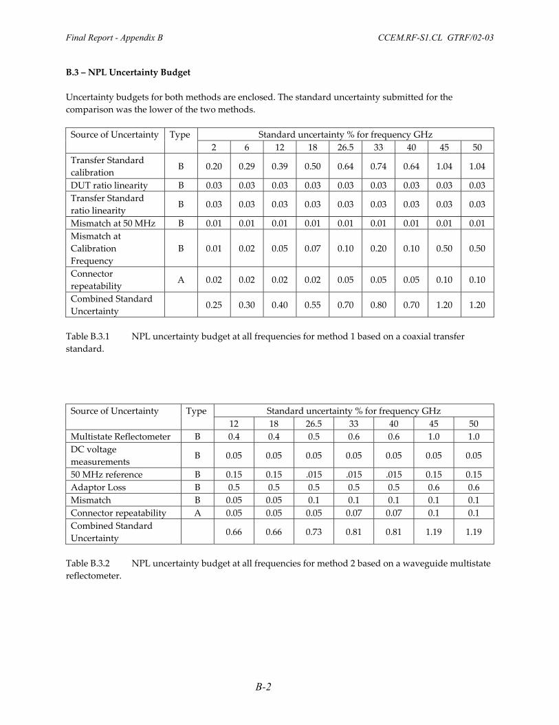
B.3 – NPL Uncertainty Budget Uncertainty budgets for both methods are enclosed. The standard uncertainty submitted for the comparison was the lower of the two methods.

Standard uncertainty % for frequency GHz Source of Uncertainty Type 2 6 12 18 26.5 33 40 45 50

Transfer Standard calibration B 0.20 0.29 0.39 0.50 0.64 0.74 0.64 1.04 1.04

DUT ratio linearity B 0.03 0.03 0.03 0.03 0.03 0.03 0.03 0.03 0.03 Transfer Standard ratio linearity

B 0.03 0.03 0.03 0.03 0.03 0.03 0.03 0.03 0.03

Mismatch at 50 MHz B 0.01 0.01 0.01 0.01 0.01 0.01 0.01 0.01 0.01 Mismatch at Calibration Frequency

B 0.01 0.02 0.05 0.07 0.10 0.20 0.10 0.50 0.50

Connector repeatability

A 0.02 0.02 0.02 0.02 0.05 0.05 0.05 0.10 0.10

Combined Standard Uncertainty

0.25 0.30 0.40 0.55 0.70 0.80 0.70 1.20 1.20

Table B.3.1 NPL uncertainty budget at all frequencies for method 1 based on a coaxial transfer standard.

Standard uncertainty % for frequency GHz Source of Uncertainty Type 12 18 26.5 33 40 45 50

Multistate Reflectometer B 0.4 0.4 0.5 0.6 0.6 1.0 1.0 DC voltage measurements

B 0.05 0.05 0.05 0.05 0.05 0.05 0.05

50 MHz reference B 0.15 0.15 .015 .015 .015 0.15 0.15 Adaptor Loss B 0.5 0.5 0.5 0.5 0.5 0.6 0.6 Mismatch B 0.05 0.05 0.1 0.1 0.1 0.1 0.1 Connector repeatability A 0.05 0.05 0.05 0.07 0.07 0.1 0.1 Combined Standard Uncertainty

0.66 0.66 0.73 0.81 0.81 1.19 1.19

Table B.3.2 NPL uncertainty budget at all frequencies for method 2 based on a waveguide multistate reflectometer.

B-2


B.4 VSL Uncertainty Budget The basic formula for obtaining the calibration factor Kx of the DUT is

CCrCs

xssx ppp

MM

KKK ,, ****)( δ+=

with Ks = calibration factor referred to 50 MHz of the standard δKs = change in calibration factor Ks due to drift Ms = mismatch factor of the standard at the calibration frequency fc Mx = mismatch factor of the DUT at the calibration frequency fc pCr = correction of the observed ratio for non-linearity and limited resolution of the power ratio level at the reference frequency of 50 MHz pCc = correction of the observed ratio for non-linearity and limited resolution of the power ratio level at the calibration frequency fc

Quantity Value Stated

uncertainty Evalu-ation

method

k= Standard uncertainty

Sensitivity Contr. To Unc.

Degreesof

freedomKs 0.996 0.007 B 2 0.0035 1.0006 0.0035 100

dKs 0.0000 0.0020 B 1 0.0020 1.0006 0.0020 100 Ms 1.0000 0.0020 B 1 0.0020 0.9966 0.0020 100 Mx 1.0000 0.0020 B 1 0.0020 -0.9966 -0.0020 100

pcr 1.0000 0.0001 B 1 0.0001 0.9999 0.0001 100 pcc 1.0000 0.0001 B 1 0.0001 0.9999 0.0001 100 p 1.0006 0.0007 A 1 0.0007 0.9993 0.0007 5

Kx 0.9966 k=1 0.0050 301

Table B.4.1 VSL uncertainty budget at 2 GHz for device 3629 Quantity Value Stated

uncertainty Evalu-ation

method

k= Standard uncertainty

Sensitivity Contr. To Unc.

Degrees of

freedom Ks 0.93 0.021 B 2 0.0105 1.0047 0.0105 100

dKs 0.0000 0.0020 B 1 0.0020 1.0047 0.0020 100

Ms 1.0018 0.0020 B 1 0.0020 0.9327 0.0019 100

Mx 1.0004 0.0020 B 1 0.0020 -0.9340 -0.0019 100

pcr 1.0000 0.0001 B 1 0.0001 0.9999 0.0001 100

pcc 1.0000 0.0001 B 1 0.0001 0.9999 0.0001 100

p 1.0032 0.0022 A 1 0.0022 0.9967 0.0022 5

Kx 0.9343 k=1 0.0113 125

Table B.4.2 VSL uncertainty budget at 40 GHz for device 3629

B-3


B.5 METAS Uncertainty Budget Uncertainty Budget GT-RF-S1.CL One Standard Deviation (k = 1) Frequency: 50 GHz Power Sensor 1 (Agilent 8487A thermocouple, sn 3318A03629, NIST 929823 ) Source of Uncertainty Type Probab.Distrib

. Sensit.Coeff. Uncertainty contribution

Power Standard Calibration Factor (NPL, 1/2000) B normal ≈ 1 0.0150Aging of Power Standard Calibration Factor B rectangular ≈ 1 0.0015Powermeter Instrumentation, 50 MHz Calibration B rectangular ≈ 1 0.0017Mismatch-Uncertainty B U-shaped ≈ 1 0.0018Connector Repeatability Standard A normal ≈ 1 0.0029Connector Repeatability DUT A normal ≈ 1 0.0020

Combined Standard Uncertainty = 0.0157

Table B.5.1 METAS' detailed uncertainty budget for 50 GHz for device 3629. Uncertainty Budget GT-RF-S1.CL Power Sensor 1 (8487A, sn 3318A03629, NIST 929823 ) Frequency: 2 6 18 26.5 33 40 45 50 Source of Uncertainty Unc.

Contrib.Unc.

Contrib.Unc.

Contrib.Unc.

Contrib.Unc.

Contrib.Unc.

Contrib. Unc.

Contrib.Unc.

Contrib.Power Standard Calibration Factor 0.0040 0.0060 0.0070 0.0075 0.0105 0.0105 0.0150 0.0150Aging of Power Standard CalFac 0.0015 0.0015 0.0015 0.0015 0.0015 0.0015 0.0015 0.0015Powermeter Instrumentation, 50 MHz Calibration

0.0017 0.0017 0.0017 0.0017 0.0017 0.0017 0.0017 0.0017

Mismatch-Uncertainty 0.0018 0.0018 0.0018 0.0018 0.0018 0.0018 0.0018 0.0018Connector Repeatability Standard 0.0001 0.0001 0.0001 0.0001 0.0002 0.0003 0.0017 0.0029Connector Repeatability DUT 0.0002 0.0002 0.0002 0.0001 0.0002 0.0004 0.0003 0.0020Combined Standard Uncertainty (One Standard Deviation)

0.0050 0.0067 0.0076 0.0080 0.0109 0.0109 0.0154 0.0157

Table B.5.2 METAS uncertainty budget at 8 frequencies for device 3629

B-4


B.6 INMS Uncertainty Budget

International Comparison GT-RF.S1.CL: NRC / INMS Measurement Report Uncertainity Budget of the 2 GHz Measurement

MeasurandComponent Data in units of the uncertainity component parameter Components

x ci U(xi) u(xi) ∆u/u ν νeff u (y)

# Component Type Name Dist std_Fac Sen Unc Std Unc du/u DF eff DF Std Unc StdUnc^2 ui^4 /vi

1Calorimeter resistance B u 0.58 1 1000.0 580 0.50 2.0 2.0 580.00 336400.00 6E+10 See note

2 Calorimeter DC Power B u 0.58 1 1000.0 580.00 0.50 2.0 2.0 580.00 336400.00 6E+10 See note

3 Att. of Calorimeter input Lines B n 1 1 2000.0 2000.00 0.50 2.0 2.0 2000.00 4000000.00 8E+12 See note

4RF-DC Current Distribution in Calorimeter B n 1 1 150.0 150.00 0.50 2.0 2.0 150.00 22500.00 3E+08 See note

5 Mismatch B n 1 1 500.0 500.0 0.25 30.0 30.0 500.00 250000 2E+09 See note

6Attenuation of Adaptor B u 0.58 1 4000.0 2320.0 0.50 2.0 2.0 2320.00 5382400 1E+13 See note

7Transfer Standard repeatability (stability) B n 1 1 1500.0 1500.0 0.25 3.0 3.0 1500.00 2250000.00 2E+12 See note

8Transfer Standard / Calorimeter (disconnects) A n 1 1 500.0 500.0 NA 4 4.0 500.00 250000.00 2E+10 See note

9Transfer Standard / Calorimeter (readings) A n 1 1 200.0 200.0 NA 4 4.0 200.00 40000.00 4E+08 See note

A Transfer Standard / DUT (disconnects) A n 1 1 500.0 500.0 NA 3 3.0 500.00 250000.00 2E+10 See note

B Transfer Standard / DUT (readings) A n 1 1 200.0 200.0 NA 3 3.0 200.00 40000.00 5E+08 See note

C "Normalization" B n 1 1 2500.0 2500.0 0.20 12.5 12.5 2500.00 6250000.00 3E+12 See note

column totals νeff Uc 19407700.00 3E+13

RSS Totals 13.7 4405.4Thus a coverage factor of k= 2.16 is needed to obtain a 95% confidence

Thus the expanded uncertainity Uc=k*uc is given by Uc = 9517 with 13.7 degrees of freedomand a coverage factor of k= 2.2 which implies probability of 95% for the +/- Uc interval

# Notes123456789

ABC

Based on the uncertainty on the Reflection Coefficients and source impedance. Based on the uncertainty on the transmission of the adapter. The repeatibility and the drift of the transfer standard over a medium period of time.

Note: All values expressed in 1e-6

Measurement of the DC input resistance of the calorimeter including the resistance of the connectorMeasurement of the DC power to the calorimeter including the shunt resistor and transfer standard and bias tee series resistor Attenuation of Calorimeter Input Lines at the frequency of measurementRF-DC current distribution inside the calorimeter. At the measurement frequency vs at DC.

A set of 16 "OFF-ON-OFF" readings are done between the disconnects. This is the contribution to the total uncertainty

A series of five disconnects are done when the Calorimeter is applied on the Transfer standard

This is the "normalization" factor in equation 2 of the protocol

A set of 6 "OFF-ON-OFF" readings are done between the disconnects. This is the contribution to the total uncertaintyA series of 4 disconnects are done when the DUT is applied on the Transfer standard

Table B.6.1 INMS uncertainty Budget at 2 GHz.

B-5


International Comparison GT-RF.S1.CL: NRC / INMS Measurement Report Uncertainity Budget of the 40 GHz Measurement

MeasurandComponent Data in units of the uncertainity component parameter Components

x ci U(xi) u(xi) ∆u/u ν νeff u (y)

# Component TypeName Dist std_Fac Sen Unc Std Unc du/u DF eff DF Std Unc StdUnc^2 ui^4 /vi

1 NORMALIZATION B n 1 1 2500.0 2500.00 0.20 12.5 12.5 2500.00 6250000.00 3E+12 See note

2 Calorimeter DC Power B u 0.58 1 20000.0 11600.00 0.50 2.0 2.0 11600.00 134560000.00 9E+15 See note

3 BLANK B n 1 1 0.0 0.00 0.50 2.0 2.0 0.00 0.00 0E+00 See note4 BLANK B n 1 1 0.0 0.00 0.25 8.0 8.0 0.00 0.00 0E+00 See note5 Mismatch B Refl n 1 1 2000.0 2000.0 0.25 30.0 30.0 2000.00 4000000 5E+11 See note

6Attenuation of Adaptor B Refl n 1 1 10000.0 10000.0 0.25 8.0 8.0 10000.00 100000000 1E+15 See note

7Transfer Standard repeatability (stability) B n 1 1 2000.0 2000.0 0.25 3.0 3.0 2000.00 4000000.00 5E+12 See note

8Transfer Standard / Calorimeter (disconnects) A n 1 1 2000.0 2000.0 NA 4 4.0 2000.00 4000000.00 4E+12 See note

9Transfer Standard / Calorimeter (readings) A n 1 1 200.0 200.0 NA 4 4.0 200.00 40000.00 4E+08 See note

A Transfer Standard / DUT (disconnects) A n 1 1 1500.0 1500.0 NA 4 4.0 1500.00 2250000.00 1E+12 See note

B Transfer Standard / DUT (readings) A n 1 1 200.0 200.0 NA 24 24.0 200.00 40000.00 7E+07 See note

column totals νeff Uc 255140000.00 1E+16

RSS Totals 6.3 15973.1Thus a coverage factor of k= 2.45 is needed to obtain a 95% confidence

Thus the expanded uncertainity Uc=k*uc is given by Uc = 39085 with 6.3 degrees of freedomand a coverage factor of k= 2.4 which implies probability of 95% for the +/- Uc interval

# Notes123456789

AB

The repeatibility and the drift of the transfer standard over a medium period of time.

Note: All values expressed in 1e-6

A series of five disconnects are done when the "Calorimeter mount" is applied on the Transfer standard



This is the "normalization" factor in equation 2 of the protocolMeasurement of the DC power to the calorimeter including the shunt resistor and transfer standard and bias tee series resistor

A series of 6 disconnects are done when the DUT is applied on the Transfer standard

Based on the uncertainty on the Reflection Coefficients and source impedance. Based on the uncertainty on the transmission of the adapter.

Table B.6.2 INMS uncertainty Budget at 40 GHz.

B-6


B.7 CSIR Uncertainty Budget

Table B.7.1 CSIR uncertainty budget for device 3629 at 2 GHz.

B-7


Table B.7.2 CSIR uncertainty budget for device 3629 at 40 GHz.

B-8


B.8 – NMIA Uncertainty Budget In the uncertainty budget below: uref is the uncertainty of the calibration factor of the reference thermistor mounts; uadp is the uncertainty associated with the adaptor measurement; upm is the uncertainty attributed to measuring the ratio of indicated powers; uopt is the uncertainty attributed to measuring the output tracking of the splitter; ueqMisMatch is the equivalent mismatch uncertainty; ucon is the type A uncertainty associated with repeated measurements, including connector repeatability; ucomb is the combined standard uncertainty and is the RSS value of all the above components (k=1). Frequency

(GHz) uref

Type B uadp

Type A,B upm

Type A,B uopt

Type A,B ueqMisMatch Type B

ucon Type A

ucomb

2 0.0015 0.0022 0.0009 0.0006 0.00021 0.0008 0.0030 6 0.0020 0.0030 0.0009 0.0011 0.00024 0.0009 0.0040

18 0.0035 0.0040 0.0009 0.0024 0.00031 0.0010 0.0060 26.5 0.0056 0.0060 0.0012 0.0029 0.00041 0.0011 0.0089 33 0.0056 0.0062 0.0012 0.0030 0.00043 0.0012 0.0090 40 0.0056 0.0064 0.0012 0.0031 0.00045 0.0014 0.0092

Table B.8 NMIA uncertainty budget at all frequencies.

B-9


B.9 – NMIJ Uncertainty Budget

Table B.9.1 NMIJ uncertainty budget for device 3629 at 2 GHz.

B-10


Table B.9.2 NMIJ uncertainty budget for device 3629 at 40 GHz.

B-11


B.10 KRISS Uncertainty Budget 3318A03629 Frequency : 2 GHz

Sources of uncertainty Type Probability distribution

Standard uncertainty

(ui)

Sensitivity factor (Ci)

ui X Ci

Calibration factor of the transfer standard 1

B Normal 0.0009 0.9928 0.0009


B Normal 0.0009 0.9926 0.0009

Power ratio of the transfer standard 1

B Normal 0.0005 1.1689 0.0006


B Normal 0.0003 1.1707 0.0004

Power ratio of the traveling standard

B Normal 0.0005 1.1611 0.0006

Mismatch between the transfer std. 1 and traveling std.

B Normal 0.0004 0.9829 0.0004


B Normal 0.0003 0.9835 0.0003

Measurement repeatability

A Normal 0.0006 1.0000 0.0006

Adapter efficiency B Rectangular 0.0030 1.0000 0.0030

Combined uncertainty (1 standard deviation)

0.0036

Table B.10.1 KRISS uncertainty budget for device 3629 at 2 GHz.

B-12


B-13

3318A03629 Frequency : 40.0 GHz

Sources of uncertainty Type Probability distribution

Standard uncertainty

(ui)

Sensitivity factor (Ci)

ui X Ci


B Normal 0.0033 0.9629 0.0032


B Normal 0.0029 0.9504 0.0028


B Normal 0.0003 0.8794 0.0003


B Normal 0.0004 0.8591 0.0003

Power ratio of the traveling standard

B Normal 0.0007 0.8529 0.0006


B Normal 0.0023 0.9033 0.0021


B Normal 0.0033 0.9384 0.0031

Measurement repeatability

A Normal 0.0010 1.0000 0.0010

Adapter efficiency B Rectangular 0.0050 1.0000 0.0050

Combined uncertainty (1 standard deviation)

0.0077

Table B.10.2 KRISS uncertainty budget for device 3629 at 40 GHz.

Protocol for CCEM.RF-S1.CL GTRF/ 02- 03 RF Power Measurements with 2.4 mm Connectors

1. Traveling StandardsThe traveling standards will consist of two Agilent 8487A thermocouple

power sensors and a Hewle tt Packard (now Agilen t ) 437B power me ter. All labora tories should per form measurements with this power met er.

Specifications of the thermocouple power sensors are:Operating frequency 50 MHz to 50 GHz Maximum power 300 mWMax SWR 1.5 (40-50 GHz)Size (approx) 30 mm x 39 mm x 94 mmWeigh t 140 g

Specifications for the 437B power met er are:50 MHz Power reference 1.00 mWLine Voltage 100,120, 220, 240 VAC (+5% to -10%)Line Frequency 48 to 66 Hz (all voltages)

360 to 440 Hz (100 or 120 VAC)Remote Operation HP-IB Weigh t 2.6 kgSize 88 mm (H) x 212 mm (W) x 273 mm (D)

Further details for the power sensors can be found at h t tp:/ / cp.literature.agilent.com/ litweb /pdf /5965-6382E.pdfThe power meter manual is at h t tp:/ / cp.literature.agilent.com/ litweb /pdf /00437-90047.pdf

Final Report - Appendix C CCEM.RF-S1.CL GTRF/02-03

C-1

2. Measurements to be PerformedThe calibrat ion factor of the sensor relat ive to its 50 MHz value will be

measured by each laboratory. This quant i ty is expressed in equation (2) below. Calibration factor K is def ined as the ra tio of the power met er reading at a given f requency, Pmeter to the incident RF power, Pinc, on the sensor

K fP f

P fmeter

inc

( )( )

( )= . ( 1)

The value obtained for Pmeter depends on the sett ing of the power meter

electronics and is therefore arbitrary. The electronics are set using a calibration procedure in which a 50 MHz, 1 mW output signal from the power me ter is used as a sensor input. At the pilot laboratory, the reference calibrat ion factor is set to 100% which in turn set s the power met er electronics to yield Pmeter,ref =

Pinc,ref where the ref subscript indicates measurements made at the reference

f requency of 50 MHz. Part icipating laboratories do not need to follow this same procedure. However, in order to compare results, all measurement values sent report ed should be the relative calibrat ion factor, Krel:

K fK f

K

P f

P f

P

Prelref

meter

inc

inc ref

meter ref

( )( ) ( )

( ),

,

= = ( 2)

and the measurements at a given frequency need to be taken with the same power meter set t ings as the reference measurement. The measurement t echnique is lef t to the discretion of each participant, but it should match their normal calibrat ion service method as much as possible.

The measurements will be will be performed at the following frequencies: 2, 6, 18, 26.5, 33, 40, 45 and 50 GHz. Since not all participants will be able to make measurements at all frequencies, all frequencies will be considered opt ional.

The 2.4 mm connector should be tightened with a torque wrench when connecting it to the measurement syst em. A torque of 0.90 N-m is typically used (8 in-lb). Incident power levels for the measurements should be about 1 mW.


C-2

3. UncertaintyPart icipating laboratories should provide complet e information about the

principal components of the uncertainties and the total standard uncertainty for their measurement at each frequency. Uncertainties should be evaluat ed at one s tandard deviation and follow the principles in the Guide to the Expression of Uncer tainty in Measurement. Degrees of freedom need not be evaluated.

For the pilot lab, a direct comparison sys tem will be used with the principle components of the uncertainty as listed below. It is not expected that this will fi t all laboratories since some laboratories will use calorime ter measurements and adapt er corrections will be important for other labs. Thus, each lab should organize their uncer tainty budget in a way that bes t mat ches their experiment.

BPower Meter Inst rumentat ion and 50 MHz Reference Calibra tion

BDirec t Comparison Mismatch Correction

AConnector Repeatabili ty

ACalibration of Direct Comparison

BMicrocalorime ter 2.4 mm Standard

TypeSource of Uncertainty

Principle components of the uncertain ty budget for the pilot laboratory.

4. Intercomparison pat ternBoth power sensors and the power met er will be circulated together.

Each par ticipant will measure the devices and send them on to the next part icipant. Three set s of measurements will be made by the pilot lab to measure the stabili ty of the traveling standards. The individual pilot lab measurements will be presented separat ely in a final report .

The expected time required for a par ticipant to make their measurements and ship the traveling standards to the next par ticipant is 2 months. The schedule for the measurements is given in the table below.


C-3

Sept ember-October, 2004

July-August, 2004

May-June, 2004

March-April, 2004

January-February, 2004

Sept ember-December, 2003

July-August, 2003

May-June, 2003

March-April, 2003

January-February, 2003

December, 2002

Korea

United Stat es

Japan

Australia

South Africa

United Stat es

Canada

Switzerland

Netherlands

United Kingdom

United Stat es

NIST 3

KRISS

AIST

CSIRO-NML

CSIR-NML

NIST 2

NRC

metas

NMi Van Swinden

NPL

NIST 1

DatesCountryInstitution

In the event of failure of a thermocouple sensor or the power met er, the pilot lab should be contacted immediately. If one of the thermocouple sensors fail, the measurement loop will continue with the second standard only. If the power meter fails, then the measurements will continue, but each laboratory will have to use its own power me ter. Power met ers that are acceptable include Agilent E4418 or 43x series.

Each par ticipant is responsible for arranging and paying for the transport ( including where necessary customs clearance) and insurance of the devices f rom arrival in their labora tory until arrival in the subsequent laboratory. An ATA Carnet will be used for customs documenta tion.

5. ShippingOn arrival at each par ticipating laboratory, the traveling standards and

packaging will be inspected for damage during transit. The protrusion of the center conductor pin on both the power sensors and the labora tory test equipment should be checked before the measurements to prevent damage. The flat section of the center conductor pin must be recessed behind the outer conductor. The power me ter line voltage switches and fuse must also be se t properly by each par ticipant. Upon shipping the devices to the nex t laboratory,


C-4

part icipants should notif y the pilot lab and the next laboratory of the shipment. Similarly upon arrival, the previous lab and the pilot lab should be informed.

6. Report on Progress and ResultsThe measurement results should be report ed in English to the pilot

labora tory within one month of completing the measurements. A summary of the measurements should be prepared as an ASCII text file and sent to the pilot lab via email. There should be a single table listing the calibra tion factor and combined standard uncertainty for each measurement frequency.

In addi tion, par ticipants should submi t their uncertainty budgets and a brief descript ion (one or two paragraphs) of the apparatus and techniques used. These may be submi t ted either electronically or via mail. The description should be suitable for use in the final report . The names of all co-authors to the final report should be list ed. The laboratory operating conditions (i.e. temperature, humidi ty ), use of adapt ers to other connector sizes, and the traceabili ty route for the measurements must also be described.

7. Intercomparison ReportA draf t of the final report will be sent to all participat ing labs within two

months of when the last measurement is made at the pilot labora tory. The report will include a summary of the measurement technique employed at each labora tory, along with the measured values and uncertainties. Results will be presented relat ive to a comparison value that is the unweighted mean of the measurements.

8. Pilot Laboratory ContactThe pilot labora tory contact is:Tom CrowleyNIST, MC 813.01325 BroadwayBoulder, CO 80305USA1-303-497-41 33 (phone)1-303-497-39 70 (fax)[email protected]


C-5

9. List of Participating Laboratories and Contacts*

[email protected]

t .inoue@aist .go.jp

[email protected]

[email protected]

[email protected]

[email protected]

[email protected]

Geoff [email protected]

JeongHwan Kim

Takeumi Inoue

Tieren Zhang

Erik Dressler

Alain Michaud

Juerg Furrer

Jan de Vreede

Geoff Orford

South Korea

Japan

Australia

South Africa

Canada

Switzerland

Netherlands

KRISS

AIST

CSIRO-NML

CSIR-NML

NRC

metas

NPL United Kingdom

NMi Van Swinden

[email protected] CrowleyUnited Stat esNIST

email addressContactCountryLaboratory

*This is the par ticipant list as it appeared in the original protocol. Table 1 of the main repor t has an updat ed list .


C-6

ccem.rf-s1.cl (gtrf/02-03) rf power measurements with 2.4

Documents