The Marine Biological Laboratory Workshop on Molecular Evolution, July/August 2009Multiple Sequence Alignment: Steven M. Thompson

Beyond mere multiple sequence alignment:How good can you make an alignment, and so what?With a focus on MAFFT and SeaView

A session for the Workshop on Molecular Evolution,the Marine Biological Laboratory, Woods Hole, MA, U.S.A.

July 28, 2009, 7:00 to 10:00 PM

author:

Steven M. Thompson

Department of Biology,Valdosta State University, Valdosta, GA, 31698

e-mail:

stevet@bio.fsu.edu

mailing address and phone:

2538 Winnwood Circle, Valdosta, GA, 31601-7953, 229-249-9751

Steve ThompsonBioInfo 4U2538 Winnwood CircleValdosta, GA, USA 31601-7953stevet@bio.fsu.edu229-249-9751 2009 BioInfo 4U

2

Beyond mere multiple sequence alignment:How good can you make an alignment, and so what? With a focus on MAFFT and SeaView

Introduction

What can we know about a biological molecule, given its nucleotide or amino acid sequence? We may be able to

learn about it by searching for particular patterns within it that may reflect some function, such as the many motifs

ascribed to catalytic activity; we can look at its overall content and composition, such as do several of the gene

finding algorithms; we can map its restriction enzyme or protease cut sites; and on and on. However, what about

comparisons with other sequences? Is this worthwhile? Yes, naturally it is — inference through homology is

fundamental to all the biological sciences. We can learn a tremendous amount by comparing and aligning our

sequence against others.

Furthermore, the power and sensitivity of sequence based computational methods dramatically increase with the

addition of more data. More data yields stronger analyses — if done carefully! Otherwise, it can confound the

issue. The patterns of conservation become ever clearer by comparing the conserved portions of sequences

amongst a larger and larger dataset. Those areas most resistant to change are most important to the molecule.

The basic assumption is that those portions of sequence of crucial structural and functional value are most

constrained against evolutionary change. They will not tolerate many mutations. Not that mutation does not

occur in these regions, just that most mutation in the area is lethal, so we never see it. Other areas of sequence

are able to drift more readily, being less subject to this evolutionary pressure. Therefore, sequences end up a

mosaic of quickly and slowly changing regions over evolutionary time.

However, in order to learn anything by comparing sequences, we need to know how to compare them. We can

use those constrained portions as ‘anchors’ to create a sequence alignment allowing comparison, but this brings

up the alignment problem and ‘similarity.’ It is easy to see that sequences are aligned when they have identical

symbols at identical positions, but what happens when symbols are not identical, or the sequences are not the

same length. How can we know when the most similar portions of our sequences are aligned, when is an

alignment optimal, and does optimal mean biologically correct?

A ‘brute force,’ naïve approach just won’t work. Even without considering the introduction of gaps, the

computation required to compare all possible alignments between just two sequences requires time proportional

to the product of the lengths of the two sequences. Therefore, if two sequences are approximately the same

length (N), this is a N2 problem. The calculation would have to repeated 2N times to examine the possibility of

gaps at each possible position within the sequences, now a N4N problem. Waterman (1989) pointed out that using

this naïve approach to align two sequences, each 300 symbols long, would require1088 comparisons, more than

the number of elementary particles estimated to exist in the universe, and clearly impossible to solve! Part of the

solution to this problem is the dynamic programming algorithm, as applied to sequence alignment. Therefore,

we’ll quickly review how dynamic programming can be used to align just two sequences first.

Dynamic programming

3

Dynamic programming is a widely applied computer science technique, often used in many disciplines whenever

optimal substructure solutions can provide an optimal overall solution. I’ll illustrate the technique applied to

sequence alignment using an overly simplified gap penalty function. Matching sequence characters will be worth

one point, non-matching symbols will be worth zero points, and the scoring scheme will be penalized by

subtracting one point for every gap inserted, unless those gaps are at the beginning or end of the sequence. In

other words, end gaps will not be penalized; therefore, both sequences do not have to begin or end at the same

point in the alignment.

This zero penalty end-weighting scheme is the default for most alignment programs, but can often be changed

with program options, if desired. However, the linear gap function described here, and used in my example, is a

simpler gap penalty function than normally used in alignment programs. Usually an ‘affine,’ function (Gotoh,

1982) is used, the standard ‘y = mx + b’ equation for a line that does not cross the X,Y origin, where ‘b,’ the Y

intercept, describes how much initial penalty is imposed for creating each new gap:

total penalty = ( [ length of gap ] * [ gap extension penalty ] ) + gap opening penalty

To run most alignment programs with the type of simple linear DNA gap penalty used in my example, you would

have to designate a gap ‘creation’ or ‘opening’ penalty of zero, and a gap ‘extension’ penalty of whatever counts

in that particular program as an identical base match for DNA sequences.

My example uses two random sequences that fit the TATA promoter region consensus of eukaryotes and of

bacteria. The most conserved bases within the consensus are capitalized by convention. The eukaryote

promoter sequence is along the X-axis, and the bacterial sequence is along the Y-axis in my example.

The solution occurs in two stages. The first begins very much like dot matrix (dot plot) methods; the second is

totally different. Instead of calculating the ‘score matrix’ on the fly, as is often taught as one proceeds through the

graph, I like to completely fill in an original ‘match matrix’ first, and then add points to those positions that produce

favorable alignments next. I also like to illustrate the process working through the cells, in spite of the fact that

many authors prefer to work through the edges; they are equivalent. Points are added based on a “looking-back-

over-your-left-shoulder” algorithm rule where the only allowable trace-back is diagonally behind and above. The

illustration is shown on the following page in Table 1.

4

Table 1. Pairwise alignment with a linear gap cost

a) First complete a match matrix using one point for

matching and zero points for mismatching between

bases, just like in the previous example:

c T A T A t A a g gc 1 0 0 0 0 0 0 0 0 0g 0 0 0 0 0 0 0 0 1 1T 0 1 0 1 0 1 0 0 0 0A 0 0 1 0 1 0 1 1 0 0t 0 1 0 1 0 1 0 0 0 0A 0 0 1 0 1 0 1 1 0 0a 0 0 1 0 1 0 1 1 0 0T 0 1 0 1 0 1 0 0 0 0

b) Now add and subtract points based on the best path

through the matrix, working diagonally, left to right and

top to bottom. However, when you have to jump a box

to make the path, subtract one point per box jumped,

except at the beginning or end of the alignment, so that

end gaps are not penalized. Fill in all additions and

subtractions, calculate the sums and differences as you

go, and keep track of the best paths. My score matrix is

shown with all calculations below:

c T A T A t A a g gc 1 0 0 0 0 0 0 0 0 0g 0 0+1

=10+0-0=0

0+0-0=0

0+0-0=0

0+0-0=0

0+0-0=0

0+0-0=0

1+0-0=1

1+0=1

T 01+1-1=1

0+1=1

1+0 or+1-1=1

0+0-0=0

1+0-0=1

0+0-0=0

0+0-0=0

0+0-0=0

0+1=1

A 00+0-0=0

1+1=2

0+1=1

1+1=2

0+1-1=0

1+1=2

1+1-1=1

0+0-0=0

0+0-0=0

t 01+0-0=1

0+1-1=0

1+2=3

0+1=1

1+2=3

0+2-1=1

0+2=2

0+1=1

0+0-0=0

A 00+0-0=0

1+1=2

0+2-1=1

1+3=4

0+3-1=2

1+3=4

1+3-1=3

0+2=2

0+1=1

a 00+0-0=0

1+0-0=1

0+2=2

1+3-1=3

0+4=4

1+4-1=4

1+4=5

0+3=3

0+2=2

T 01+0-0=1

0+0-0=0

1+1=2

0+2=2

1+3=4

0+4=4

0+4=4

0+5=5

0+5-1=4

c) Clean up the score matrix next. I’ll only show the totals in each cell in the matrix shown below. All paths are highlighted:

c T A T A t A a g gc 1 0 0 0 0 0 0 0 0 0g 0 1 0 0 0 0 0 0 1 1T 0 1 1 1 0 1 0 0 0 1A 0 0 2 1 2 0 2 1 0 0t 0 1 0 3 1 3 1 2 1 0A 0 0 2 1 4 2 4 3 2 1a 0 0 1 2 3 4 4 5 3 2T 0 1 0 2 2 4 4 4 5 4

d) Finally, convert the score matrix into a trace-back path graph by picking the bottom-most, furthest right and highest scoring coordinate. Then choose the trace-back route that got you there, to connect the cells all the way back to the beginning using the same ‘over-your-left-shoulder’ rule. Only the two best trace-back routes are now highlighted with outline font in the trace-back matrix below:

c T A T A t A a g gc 1 0 0 0 0 0 0 0 0 0g 0 1 0 0 0 0 0 0 1 1T 0 1 1 1 0 1 0 0 0 1A 0 0 2 1 2 0 2 1 0 0t 0 1 0 3 1 3 1 2 1 0A 0 0 2 1 4 2 4 3 2 1a 0 0 1 2 3 4 4 5 3 2T 0 1 0 2 2 4 4 4 5 4

These two trace-back routes define the

following two alignments:

cTATAtAagg cTATAtAagg| ||||| and |||||cg.TAtAaT. .cgTAtAaT.

5

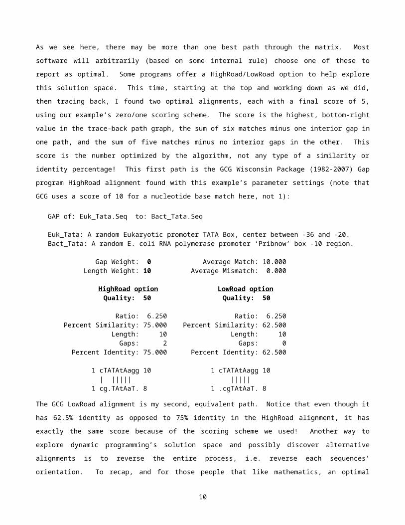
As we see here, there may be more than one best path through the matrix. Most software will arbitrarily (based

on some internal rule) choose one of these to report as optimal. Some programs offer a HighRoad/LowRoad

option to help explore this solution space. This time, starting at the top and working down as we did, then tracing

back, I found two optimal alignments, each with a final score of 5, using our example’s zero/one scoring scheme.

The score is the highest, bottom-right value in the trace-back path graph, the sum of six matches minus one

interior gap in one path, and the sum of five matches minus no interior gaps in the other. This score is the

number optimized by the algorithm, not any type of a similarity or identity percentage! This first path is the GCG

Wisconsin Package (1982-2007) Gap program HighRoad alignment found with this example’s parameter settings

(note that GCG uses a score of 10 for a nucleotide base match here, not 1):

GAP of: Euk_Tata.Seq to: Bact_Tata.Seq

Euk_Tata: A random Eukaryotic promoter TATA Box, center between -36 and -20.Bact_Tata: A random E. coli RNA polymerase promoter ‘Pribnow’ box -10 region.

Gap Weight: 0 Average Match: 10.000 Length Weight: 10 Average Mismatch: 0.000

HighRoad option LowRoad option Quality: 50 Quality: 50

Ratio: 6.250 Ratio: 6.250 Percent Similarity: 75.000 Percent Similarity: 62.500 Length: 10 Length: 10 Gaps: 2 Gaps: 0 Percent Identity: 75.000 Percent Identity: 62.500

1 cTATAtAagg 10 1 cTATAtAagg 10 | ||||| ||||| 1 cg.TAtAaT. 8 1 .cgTAtAaT. 8

The GCG LowRoad alignment is my second, equivalent path. Notice that even though it has 62.5% identity as

opposed to 75% identity in the HighRoad alignment, it has exactly the same score because of the scoring scheme

we used! Another way to explore dynamic programming’s solution space and possibly discover alternative

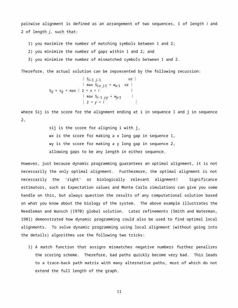
alignments is to reverse the entire process, i.e. reverse each sequences’ orientation. To recap, and for those

people that like mathematics, an optimal pairwise alignment is defined as an arrangement of two sequences, 1 of

length i and 2 of length j, such that:

1) you maximize the number of matching symbols between 1 and 2;

2) you minimize the number of gaps within 1 and 2; and

3) you minimize the number of mismatched symbols between 1 and 2.

Therefore, the actual solution can be represented by the following recursion:

Si-1 j-1 or max Si-x j-1 + wx-1 or Sij = sij + max 2 < x < i max Si-1 j-y + wy-1 2 < y < i

6

where Sij is the score for the alignment ending at i in sequence 1 and j in sequence 2,

sij is the score for aligning i with j,

wx is the score for making a x long gap in sequence 1,

wy is the score for making a y long gap in sequence 2,

allowing gaps to be any length in either sequence.

However, just because dynamic programming guarantees an optimal alignment, it is not necessarily the only

optimal alignment. Furthermore, the optimal alignment is not necessarily the ‘right’ or biologically relevant

alignment! Significance estimators, such as Expectation values and Monte Carlo simulations can give you some

handle on this, but always question the results of any computational solution based on what you know about the

biology of the system. The above example illustrates the Needleman and Wunsch (1970) global solution. Later

refinements (Smith and Waterman, 1981) demonstrated how dynamic programming could also be used to find

optimal local alignments. To solve dynamic programming using local alignment (without going into the details)

algorithms use the following two tricks:

1) A match function that assigns mismatches negative numbers further penalizes the scoring scheme.

Therefore, bad paths quickly become very bad. This leads to a trace-back path matrix with many

alternative paths, most of which do not extend the full length of the graph.

2) The best trace-back within the overall graph is chosen. This does not have to begin or end at the edges

of the matrix — it’s the best segment of alignment.

Significance

The discrimination between homology and similarity is particularly misunderstood — there is a huge difference!

Similarity is merely a statistical parameter that describes how much two sequences, or portions of them, are alike

according to some set scoring criteria. It can be normalized to ascertain statistical significance as in database

searching methods, but it’s still just a number. Homology, in contrast and by definition, implies an evolutionary

relationship — more than just the fact that all life evolved from the same primordial ‘slime.’ You need to be able to

demonstrate some type of evolutionary lineage between the organisms or genes of interest in order to claim

homology. Better yet, demonstrate experimental evidence, structural, morphological, genetic, or fossil, that

corroborates your assertion. There really is no such thing as percent homology; something is either homologous

or it’s not. Walter Fitch (personal communication) explains with the joke, “homology is like pregnancy — you can’t

be 45% pregnant, just like something can’t be 45% homologous. You either are or you are not.” Do not make the

mistake of calling any old sequence similarity homology. Highly significant similarity can argue for homology, not

the other way around.

So, how do you tell if a similarity, in other words, an alignment discovered by some program, means anything? Is

it statistically significant, is it truly homologous, and even more importantly, does it have anything to do with real

biology? Many programs generate percent similarity scores; however, as seen in the TATA example above,

these really don’t mean a whole lot. Don’t use percent similarities or identities to compare sequences except in

the roughest way. They are not optimized or normalized in any manner. Quality scores mean a lot more but are

difficult to interpret. At least they take the length of similarity, all of the necessary gaps introduced, and the

7

matching of symbols all into account, but quality scores are only relevant within the context of a particular

comparison or search. The quality ratio is the metric optimized by dynamic programming divided by the length of

the shorter sequence. As such it represents a fairer comparison metric, but it also is relative to the particular

scoring matrix and gap penalties used in the procedure.

A traditional way of deciding alignment significance relies on an old statistics trick — Monte Carlo simulations.

This type of significance estimation has implicit statistical problems; however, few practical alternatives exist for

just comparing two sequences, and they are fast and easy to perform. Monte Carlo randomization options in

dynamic programming alignment algorithms compare an actual score, in this case the quality score of an

alignment, against the distribution of scores of alignments of a randomized sequence. These options randomize

your sequence at least 100 times after the initial alignment and then generate the jumbled alignment scores and a

standard deviation based on their distribution. Comparing the mean of the randomized sequence alignment

scores to the original score using a ‘Z score’ calculation can help you decide significance. An old ‘rule-of-thumb’

is if the actual score is much more than three standard deviations above the mean of the randomized scores, the

analysis may be significant; if it is much more than five, than it probably is significant; and if it is above nine, than it

definitely is significant. Many Z scores measure this distance from the mean using a simplistic Monte Carlo model

assuming a normal Gaussian distribution, in spite of the fact that ‘sequence-space’ actually follows an ‘extreme

value distribution;’ however, this simplistic approximation estimates significance quite well:

Z score = [ ( actual score ) - ( mean of randomized scores ) ] ( standard deviation of randomized score distribution )

When the two TATA sequences from the previous dynamic programming example are compared to one another

using the same scoring parameters as before, but incorporating a Monte Carlo Z score calculation, their similarity

is found to be not at all significant. The mean score based on 100 randomizations was 41.8 +/- a standard

deviation of 7.4. Plugged into the formula: ( 50 – 41.8 ) / 7.4 = 1.11, i.e. there is no significance to the match in

spite of 75% identity! Composition can make a huge difference — the similarity is merely a reflection of the

relative abundance of A’s and T’s in the sequences!

Most modern database similarity searching algorithms, including FastA (Pearson and Lipman, 1988, and Pearson,

1998), BLAST (Altschul, et al., 1990, and Altschul, et al., 1997), Profile (Gribskov, et al., 1987), and HMMer

(Eddy, 1998), use a similar approach but base their statistics on the distance of the query matches from the

actual, or a simulated, extreme value distribution of the rest of the ‘insignificantly similar,’ members of the

database being searched. For alignments without gaps, the math generalizes such that an Expectation value E

relates to a particular score S through the function E = Kmnes (Karlin and Altschul, 1990, and see

http://www.ncbi.nlm.nih.gov/BLAST/tutorial/Altschul-1.html). In a database search m is the length of the query

and n is the size of the database in residues. K and are supplied by statistical theory, dependent on the scoring

system and the background amino acid frequencies, and calculated from actual or simulated database alignment

distributions. Expectation values are printed in scientific notation and the smaller the number, i.e. the closer it is

to 0, the more significant the match. Expectation values show us how often we should expect a particular

alignment to occur merely by chance alone in a search of that size database. In other words, it helps to know how

8

strong an alignment can be expected from chance alone, to assess whether it constitutes evidence for homology,.

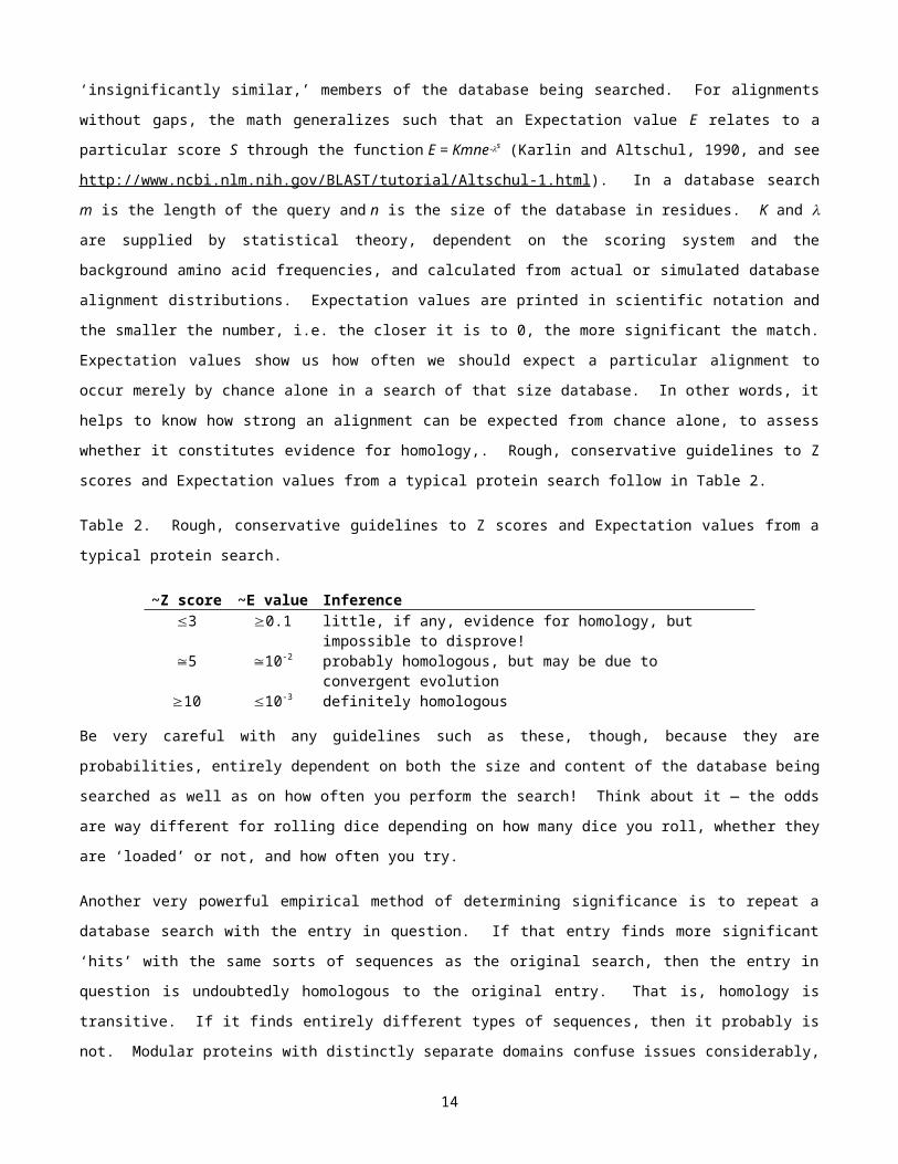
Rough, conservative guidelines to Z scores and Expectation values from a typical protein search follow in Table 2.

Table 2. Rough, conservative guidelines to Z scores and Expectation values from a typical protein search.

~Z score ~E value Inference3 0.1 little, if any, evidence for homology, but impossible to disprove!5 10-2 probably homologous, but may be due to convergent evolution10 10-3 definitely homologous

Be very careful with any guidelines such as these, though, because they are probabilities, entirely dependent on

both the size and content of the database being searched as well as on how often you perform the search! Think

about it — the odds are way different for rolling dice depending on how many dice you roll, whether they are

‘loaded’ or not, and how often you try.

Another very powerful empirical method of determining significance is to repeat a database search with the entry

in question. If that entry finds more significant ‘hits’ with the same sorts of sequences as the original search, then

the entry in question is undoubtedly homologous to the original entry. That is, homology is transitive. If it finds

entirely different types of sequences, then it probably is not. Modular proteins with distinctly separate domains

confuse issues considerably, but the principles remain the same, and can be explained through domain swapping

and other examples of non-vertical transmission. And, finally, the ‘gold-standard’ of homology is shared structural

folds — if you can demonstrate that two proteins have the same structural fold, then, regardless of similarity, at

least that particular domain is homologous between the two.

Scoring matrices

However, what about protein sequences — conservative replacements and similarities, as opposed to identities?

This is certainly an additional complication that would seem important. Particular amino acids are very much

alike, structurally, chemically, and genetically. How can we take advantage of amino acid similarity of in our

alignments? People have been struggling with this problem since the late 1960’s. Dayhoff (Schwartz and

Dayhoff, 1979) unambiguously aligned closely related protein datasets (no more than 15% difference, and in

particular cytochrome c) available at that point in time and noticed that certain residues, if they mutate at all, are

prone to change into certain other residues. As it works out, these propensities for change fell into the same

categories that chemists had known for years — those same chemical and structural classes mentioned above —

conserved through the evolutionary constraints of natural selection. Dayhoff’s empirical observation quantified

these changes. Based on the multiple sequence alignments that she created and the empirical amino acid

frequencies within those alignments, the assumption that estimated mutation rates in closely related proteins can

be extrapolated to more distant relationships, and matrix and logarithmic mathematics, she was able to empirically

specify the relative probabilities at which different residues mutated into other residues through evolutionary

history, as appropriate within some level of divergence between the sequences considered. This is the basis of

the famous PAM (corrupted acronym of ‘accepted point mutation’) 250 (meaning that the matrix has been

multiplied by itself 250 times) log odds matrix.

9

Since Dayhoff’s time other biomathematicians (eg. Henikoff and Henikoff’s [1992] BLOSUM series of matrices,

and the Gonnet et al. matrix [1992]) have created matrices regarded more accurate than Dayhoff’s original, but

the concept remains the same. Plus, Dayhoff’s original PAM 250 matrix remains a classic as historically the most

widely used amino acid substitution matrix. Confusingly these matrices are known variously as symbol

comparison, log odds, substitution, or scoring tables or matrices, and they are fundamental to all sequence

comparison techniques.

The default amino acid scoring matrix for most protein similarity comparison programs is the BLOSUM62 table

(Henikoff and Henikoff, 1992). The “62” refers to the minimum level of identity within the ungapped sequence

blocks that went into the creation of the matrix. Lower BLOSUM numbers are more appropriate for more

divergent datasets. The BLOSUM62 matrix follows below in Table 3; values whose magnitude is 4 are drawn

in shadowed characters to make them easier to recognize.

Table 3. The BLOSUM62 amino acid scoring matrix.

A B C D E F G H I K L M N P Q R S T V W X Y ZA 44 -2 0 -2 -1 -2 0 -2 -1 -1 -1 -1 -2 -1 -1 -1 1 0 0 -3 -1 -2 -1B -2 66 -3 66 2 -3 -1 -1 -3 -1 -4-4 -3 1 -1 0 -2 0 -1 -3 -4-4 -1 -3 2C 0 -3 99 -3 -4-4 -2 -3 -3 -1 -3 -1 -1 -3 -3 -3 -3 -1 -1 -1 -2 -1 -2 -4-4D -2 66 -3 66 2 -3 -1 -1 -3 -1 -4-4 -3 1 -1 0 -2 0 -1 -3 -4-4 -1 -3 2E -1 2 -4-4 2 55 -3 -2 0 -3 1 -3 -2 0 -1 2 0 0 -1 -2 -3 -1 -2 55F -2 -3 -2 -3 -3 66 -3 -1 0 -3 0 0 -3 -4-4 -3 -3 -2 -2 -1 1 -1 3 -3-3G 0 -1 -3 -1 -2 -3 66 -2 -4-4 -2 -4-4 -3 0 -2 -2 -2 0 -2 -3 -2 -1 -3 -2H -2 -1 -3 -1 0 -1 -2 88 -3 -1 -3 -2 1 -2 0 0 -1 -2 -3 -2 -1 2 0I -1 -3 -1 -3 -3 0 -4-4 -3 44 -3 2 1 -3 -3 -3 -3 -2 -1 3 -3 -1 -1 -3K -1 -1 -3 -1 1 -3 -2 -1 -3 55 -2 -1 0 -1 1 2 0 -1 -2 -3 -1 -2 1L -1 -4-4 -1 -4-4 -3 0 -4-4 -3 2 -2 44 2 -3 -3 -2 -2 -2 -1 1 -2 -1 -1 -3M -1 -3 -1 -3 -2 0 -3 -2 1 -1 2 55 -2 -2 0 -1 -1 -1 1 -1 -1 -1 -2N -2 1 -3 1 0 -3 0 1 -3 0 -3 -2 66 -2 0 0 1 0 -3 -4-4 -1 -2 0P -1 -1 -3 -1 -1 -4-4 -2 -2 -3 -1 -3 -2 -2 77 -1 -2 -1 -1 -2 -4-4 -1 -3 -1Q -1 0 -3 0 2 -3 -2 0 -3 1 -2 0 0 -1 55 1 0 -1 -2 -2 -1 -1 2R -1 -2 -3 -2 0 -3 -2 0 -3 2 -2 -1 0 -2 1 55 -1 -1 -3 -3 -1 -2 0S 1 0 -1 0 0 -2 0 -1 -2 0 -2 -1 1 -1 0 -1 44 1 -2 -3 -1 -2 0T 0 -1 -1 -1 -1 -2 -2 -2 -1 -1 -1 -1 0 -1 -1 -1 1 55 0 -2 -1 -2 -1V 0 -3 -1 -3 -2 -1 -3 -3 3 -2 1 1 -3 -2 -2 -3 -2 0 44 -3 -1 -1 -2W -3 -4-4 -2 -4-4 -3 1 -2 -2 -3 -3 -2 -1 -4-4 -4-4 -2 -3 -3 -2 -3 1111 -1 2 -3X -1 -1 -1 -1 -1 -1 -1 -1 -1 -1 -1 -1 -1 -1 -1 -1 -1 -1 -1 -1 -1 -1 -1Y -2 -3 -2 -3 -2 3 -3 2 -1 -2 -1 -1 -2 -3 -1 -2 -2 -2 -1 2 -1 77 -2Z -1 2 -4-4 2 55 -3 -2 0 -3 1 -3 -2 0 -1 2 0 0 -1 -2 -3 -1 -2 55

Notice that positive identity values range from 4 to 11, and negative values for rare substitutions go as low as -4.

The highest scoring residue is tryptophan with an identity score of 11; cysteine is next with a score of 9; histidine

gets 8; both proline and tyrosine get scores of 7. These residues get the highest scores because of two biological

factors: they are very important to the structure and function of proteins so they are the most conserved, and they

are the rarest amino acids found in nature. Also check out the hydrophobic substitution triumvirate — isoleucine,

leucine, valine, and to a lesser extent methionine — all easily swap places. So, rather than using the zero/one

match function that we used in the previous dynamic programming example, protein sequence alignments use the

10

match function provided by an amino acid scoring matrix. The concept of similarity becomes very important with

some amino acids being way ‘more similar’ than others!

Multiple sequence dynamic programming

Dynamic programming reduces the pairwise alignment problem’s complexity down to order N2 — the solution of a

two-dimensional matrix, and the complexity of the solution is equal to the length of the longest sequence squared.

But how do you work with more than just two sequences at a time? It becomes a much harder problem. You

could manually align your sequence data with an editor, but some type of an automated solution is desirable, at

least as a starting point to manual alignment. However, solving the dynamic programming algorithm for more

than just two sequences rapidly becomes intractable. Dynamic programming’s complexity, and hence its

computational requirements, increases exponentially with the number of sequences in the dataset being

compared (complexity=[sequence length]number of sequences), an N-dimensional matrix. So a three sequence

dynamic programming alignment would require the solution of a three-axis matrix, with complexity equal to the

length of the longest sequence cubed, and so forth. You can at least draw a three-dimensional matrix, but more

dimensions than that quickly become impossible to even visualize!

Several different heuristics have been employed over the years to simplify the complexity of the problem. One

classic program, MSA (Gupta et al. 1995), attempts to globally solve the N-dimensional matrix recursion using a

bounding box trick. However, the algorithm’s complexity precludes its use in most situations, except with very

small datasets. Another way to globally solve the algorithm, and yet reduce its complexity, is to restrict the search

space to only the most conserved ‘local’ portions of all the sequences involved. This approach is used by the

program PIMA (Smith and Smith, 1992). MSA and PIMA are both available through the Internet at several

bioinformatics servers (in particular see the Baylor College of Medicine’s Search Launcher at

http://searchlauncher.bcm.tmc.edu/), or they can be installed on your own machine.

Heuristic solutions — how the algorithms work

Most implementations of automated multiple alignment do not attempt to globally solve the algorithm; they modify

dynamic programming by establishing a pairwise order in which to build the alignment. This heuristic modification

is known as pairwise, progressive dynamic programming. Originally attributed to Feng and Doolittle (1987), this

variation of the dynamic programming algorithm generates a global alignment, but restricts its search space at

any one time to a local neighborhood of the full length of only two sequences. Consider a group of sequences.

First all are compared to each other, pairwise, using some quick variation of standard dynamic programming.

This establishes an order for the set, most to least similar, a ‘guide-tree’ if you will. Subgroups are clustered

together similarly. The algorithm then takes the top two, most similar sequences, and aligns them. Then it

creates a quasi-consensus of those two and aligns that to the third sequence. Next it creates the same sort of

quasi-consensus of the first three sequences and aligns that to the forth most similar. The way that the program

makes and uses this ‘consensus’ sequence is one of the biggest differences between the various

implementations. This process, all using standard, pairwise dynamic programming, continues until it has worked

its way through all of the sequences and/or sets of clusters, to complete the full multiple sequence alignment.

11

The pairwise, progressive solution is implemented in several programs. Perhaps the most popular is Higgins’ and

Thompson’s ClustalW (1994) and its multi-platform, graphical user interface ClustalX (Thompson, et al., 1997).

This program made the first major advances over the basic Feng and Doolittle algorithm by incorporating variable

sequence weighting, dynamically varying gap penalties and substitution matrices, and a neighbor-joining (NJ,

Saitou and Nei, 1987) guide-tree. ClustalX is available for most windowing operating systems — UNIX/Linux,

Microsoft (MS) Windows, and Macintosh. Complete documentation comes with the program and is accessed

through a “Help” menu. The GCG (1982–2007) program PileUp implements a similar method, but without the

later innovations, and ClustalW is also included in the GCG package.

Several more variations on the theme have come along in recent years. T-Coffee (Tree-based Consistency

Objective Function For alignment Evaluation [Notredame, et al., 2000]) was one of the first after ClustalW, and it

has gained much favor. Its biggest innovation is the use of a preprocessed, weighted library of all the pairwise

global alignments between the sequences in your dataset plus the ten best local alignments associated with each

pair of sequences. This helps build the NJ guide-tree and the progressive alignment both. Furthermore, the

library is used to assure consistency and help prevent errors, by allowing ‘forward-thinking’ to see whether the

overall alignment will be better one way or another after particular segments are aligned one way or another.

Notredame (2006) makes the apt analogy of school schedules — everybody, students, teachers and

administrators, with some folk being more important than others, i.e. the weighting factor, puts the schedule they

desire in a big pile, i.e. T-Coffee’s library, with the trick being to best fit all the schedules to one academic

calendar, so that everybody is happiest, i.e. T-Coffee’s final multiple sequence alignment. T-Coffee can even tie

together multiple methods as external modules, making consistency libraries from the results of each, as long as

all the specified methods are installed on your system. T-Coffee is one of the most accurate multiple sequence

alignment methods available because of this consistency based rationale, but it is not the fastest.

Muscle (Edgar, 2004 and 2006) is another relatively new multiple sequence alignment program. It is incredibly

fast, yet nearly as accurate as T-Coffee with protein data. Muscle is an iterative method that uses weighted log-

expectation profile scoring along with a slew of optimizations. It proceeds in three stages — draft progressive

using k-mer counting, improved progressive using a revised tree from the previous iteration, and refinement by

sequential deletion of each tree edge with subsequent profile realignment. Perhaps the most accurate new

multiple sequence alignment program is ProbCons (Do, et al., 2005). It uses Hidden Markov Model (HMM)

techniques and posterior probability matrices that compare random pairwise alignments to expected pairwise

alignments. Probability consistency transformation is used to reestimate the scores, and a guide-tree is then

constructed, which is used to compute the alignment, which is then iteratively refined.

The program that we will concentrate on today, MAFFT (Katoh, et al., 2002 and 2005, http://align.bmr.kyushu-

u.ac.jp/mafft/software/), can be run many different ways — a couple of progressive, approximate modes, using a

fast Fourier transformation (FFT); a couple of iteratively refined methods that add in weighted-sum-of-pairs (WSP)

scoring; and several iterative methods that use the WSP scoring combined with a T-Coffee-like consistency based

scoring scheme. Speed and accuracy are inversely proportional for these from fast and rough, to slow and

accurate, respectively. MAFFT provides command aliases for all of them, from fast to slow — FFTNS with or

without retree, FFTNSI with or without maxiterate, and the three combined approaches EINSI, LINSI, and GINSI.

12

MAFFT’s fast Fourier transform provide a huge speedup over most previous methods. Homologous regions are

quickly identified by converting amino acid residues to vectors of volume and polarity, thus changing a twenty-

character alphabet to six, rather than by using an amino acid similarity matrix. Similarly, nucleotide bases are

converted to vectors of imaginary and complex numbers. The FFT trick then reduces the complexity of the

subsequent comparison to Order NlogN. FFT identifies potential similarities though, without localizing them; a

sliding window step using the BLOSUM62 matrix is used for this. Then MAFFT constructs a distance matrix, and

hence a progressive guide tree, on the number of shared six-tuples from this Fourier transform, rather than on a

ranking based on full-length, pairwise sequence similarity. The user can specify how many times a new guide

tree is subsequently recalculated from a previous alignment as many times as desired; the alignment is

reconstructed using the Needlman-Wunsch algorithm for each pass.

The iterative refinement modes build on this foundation by adding steps that adjust the alignment back and forth

until there is either solely no improvement in the WSP score (or the number of cycles has reached your set limit),

or it adds both this WSP score and a T-Coffee-like consistency score between pairwise and multiple alignments to

the refinement procedure. Differences in the iterative methods that combine WSP and consistency scores are

based on how the pairwise scores are calculated, globally, locally with affine gap costs, or locally with generalized

affine gap costs. Knowing which to choose, especially if you’re dealing with sequences too diverged for the fast

methods to work well, depends on the nature of your data. MAFFT’s Algorithm page (http://align.bmr.kyushu-

u.ac.jp/mafft/software/algorithms/algorithms.html) explains where and when each mode is most appropriate. If

you know beforehand that your sequences have full-length, but low, similarity, then the global option is

appropriate (GINSI); if your sequences have one similar domain among a bunch of ‘junk,’ then the local affine gap

option works best (LINSI); whereas if your data is composed of multiple, alignable domains, then the local

generalized affine gap scheme is the way to go (EINSI).

MAFFT’s capability to handle large datasets and its speed is similar to or greater than Muscle’s in its faster

modes; its results and capabilities are similar to T-Coffee in its slow, iteratively refined, optimized modes. We’ll be

exploring MAFFT much further in the tutorial section of today’s session.

Coding DNA issues

All alignment algorithms, pairwise, multiple, and database similarity searching, are far more sensitive at the amino

acid level than at the DNA level. Twenty match symbols are just much easier to align then only four; the signal to

noise ratio is so much better. And, the concept of similarity applies to amino acids, but generally not to

nucleotides. Furthermore, many DNA base changes (especially third position changes) do not change the

encoded protein. All of these factors drastically increase the ‘noise’ level of DNA; typically giving protein similarity

searches a five to ten times greater ‘look-back’ time. Therefore, database searching and sequence alignment

should always be done on a protein level, unless you are dealing with noncoding DNA, or if the sequences are so

similar as to not cause any problems. Therefore, usually, if dealing with coding sequences, translate the DNA to

its protein counterpart, before performing multiple sequence alignment.

Even if you are dealing with very similar coding sequences, where the DNA can be directly aligned, it is often best

to align the DNA along with its corresponding proteins. In addition to the much more easily achieved alignment,

13

this also insures that alignment gaps are not placed within codons. Phylogenetic analysis can then be performed

on the DNA rather than on the proteins. This is especially important when dealing with datasets that are quite

similar, since the proteins may not reflect many differences hidden in the DNA. Furthermore, many people prefer

to run phylogenetic analyses on DNA rather than protein regardless of how similar they are — the multiple

substitution models have a long and well-accepted history, and yet are far simpler. In fact, some phylogenetic

inference algorithms do not even take advantage of amino acid similarity when dealing with protein sequences;

they only count identities, though many others can use PAM style models. However, the more diverged a dataset

becomes, the more random third and eventually first codon positions become, which introduces noise (error) into

the analysis. Therefore, often third positions and sometimes first positions are masked out of datasets. Just like

in most of computational molecular biology, one is always balancing signal against noise. Too much noise or too

little signal, both degrade the analysis to the point of nonsense.

Several scripts and programs, as well as some Web servers, can perform this sort of codon-based alignment, but

they can be a bit tricky to run. Examples include mrtrans (Pearson, 1990) (also available in EMBOSS [Rice, et al.,

2000] as tranalign and in BioPerl [Stajich et al., 2000] as aa_to_dna_aln), transAlign (Bininda-Emonds, 2005),

RevTrans (Wernersson and Pedersen, 2003), protal2dna (Letondal and Schuerer, [Pasteur Institute and in

BioPerl]), and PAL2NAL (Suyama, et al., 2006). Some multiple sequence alignment editors, including SeaView

(Galtier, et al., 1996) and GCG’s SeqLab (based on Smith’s Genetic Data Environment [GDE], 1994), can also

help with this process. We’ll use SeaView during the tutorial to illustrate the concept.

Multiple sequence alignment is much more difficult if you are forced to align nucleotides because the region does

not code for a protein. Automated methods may be able to help as a starting point, but they are certainly not

guaranteed to come up with a biologically correct alignment. The resulting alignment will probably have to be

extensively edited, if it works at all. Success will largely depend on the similarity of the nucleotide dataset.

Reliability?

One liability of most global progressive, pairwise methods is they are entirely dependent on the order in which the

sequences are aligned. Fortunately ordering them from most similar to least similar usually makes biological

sense and works quite well. However, most of the techniques are very sensitive to the substitution matrix and gap

penalties specified. Some programs allow ‘fine-tuning’ areas of an alignment by realignment with different scoring

matrices and/or gap penalties; this can be extremely helpful. However, any automated multiple sequence

alignment program should be thought of as only a tool to offer a starting alignment that can be improved upon, not

the ‘end-all-to-meet-all’ solution, guaranteed to provide the ‘one-true’ answer. Although, in this post-genomics

era, when having to deal with Giga bases of data, it does make sense to start with the ‘best’ solution possible.

This is the premise of using a very accurate multiple sequence alignment package, such as T-Coffee (Notredame,

et al., 2000), ProbCons, (Do, et al., 2005), or MAFFT (Katoh, et al., 2002 and 2005).

Regardless of the program used to create an alignment, always use comparative approaches to help assure its

reliability. After the program has offered its best guess, try to improve it further. Think about it — a sequence

alignment is a statement of positional homology — it is a hypothesis of evolutionary history. It establishes the

explicit homologous correspondence of each individual sequence position, each column in the alignment.

14

Therefore, insure that you prepare a good one — be sure that it makes sense. Editing alignments to insure that

all columns are truly homologous should be encouraged. Dedicated sequence alignment editing software such as

GCG’s SeqLab, Jalview (Clamp, et al., 2004), Se-Al (Rambaut, 1996), and the editor to be illustrated today,

SeaView (Galtier, et al., 1996, http://pbil.univ-lyon1.fr/software/seaview.html), are great for this, but any editor will

do, as long as the sequences end up properly formatted afterwards.

Devote considerable time and energy toward developing the best alignment possible. Use your understanding of

the biological system to help guide your judgment. Look for conserved functional, enzymatic, regulatory, and

structural elements and motifs — they should all line up. Searches of the PROSITE Database of protein families

and domains (Bairoch, 1992) for catalogued structural, regulatory, and enzymatic consensus patterns or

‘signatures’ in your dataset can help, as can de novo motif discovery tools like the MEME (Bailey and Elkan,

1994), MotifSearch (Bailey and Gribskov, 1998) program pair. Look for columns of strongly conserved residues

such as tryptophans, cysteines, and histidines; important structural amino acids such as prolines, tyrosines and

phenylanines; and conserved isoleucine, leucine, valine substitutions. Make subjective decisions. Is it good

enough; do things align the way they should? If, after all else, you decide that you just can’t align some region, or

an entire sequence, then get rid of it. Another alternative is to use the mask or sites selection function available in

some editors like SeaView. Cutting an entire sequence out of an alignment may leave columns of gaps across

the entire alignment that will need to be removed. Most alignment editors have a function for that. The extreme

amino- and carboxy-termini (5’ and 3’ in DNA) seldom align nicely; they are often jagged and uncertain, and

should usually be excluded. The validity of any subsequent analysis is absolutely dependent upon the quality of

your input alignment.

The conservation of co-varying sites in ribosomal and other structural RNA alignments can be very helpful in

refining alignments. That is, as one base in a stem structure changes, the corresponding Watson-Crick paired

base will change in a corresponding manner. This principle has guided the assembly of rRNA structural

alignments at the Ribosomal Database Project at Michigan State University (Cole, et al. 2007,

http://rdp.cme.msu.edu/) and at the University of Gent, Belgium, at the European Ribosomal RNA database

(Wuyts, et al. 2004, http://www.psb.ugent.be/rRNA/).

Be sure an alignment makes biological sense — align things that make sense to align! Beware of comparing

‘apples and oranges.’ Be particularly suspect of sequence datasets found through text-based database searches

such as NCBI’s Entrez, GCG’s LookUp (1982–2007), and the Sequence Retrieval System (SRS, Etzold and

Argos, 1993). For example, don’t try to align receptors and/or activators with their namesake proteins. Be wary of

trying to align genomic sequences with cDNA when working with DNA; the introns will cause all sorts of

headaches. Similarly, aligning mature and precursor proteins, or alternate splicing forms, from the same

organism and locus, doesn’t make evolutionary sense, as one is not evolved from the other, rather one is the

other. Watch for redundant sequences; there are tons of them in the databases. If creating alignments for

phylogenetic inference, either make paralogous comparisons (i.e. evolution via gene duplication) to ascertain

gene phylogenies within one organism, or orthologous (within one ancestral loci) comparisons to ascertain gene

phylogenies between organisms (which should imply organismal phylogenies). Try not to mix them up without

15

complete data representation. Otherwise, confusion can mislead interpretation, especially if the sequences’

nomenclature is inconsistent. These are all easy mistakes to make; try your best to avoid them.

Remember the old adage “garbage in — garbage out!” Some general guidelines to remember (Olsen, 1992)

include the following:

• If the homology of a region is in doubt, then throw it out.

• Avoid the most diverged parts of molecules; they are the greatest source of systematic error.

• Do not include sequences that are more diverged than necessary for the analysis at hand.

Complications

Sequence data format is a huge problem in computational molecular biology. The major databases all have their

own distinct format, plus many of the different programs and packages require their own. Clustal (Higgins, et al.,

1992) has a specific format associated with it. The FastA database similarity-searching package (Pearson and

Lipman, 1988) uses a very basic sequence format that many programs recognize. The National Center for

Biotechnology Information (NCBI) uses a library standard called ASN.1 (Abstract Syntax Notation One), plus it

provides GenBank flatfile format for all sequence data. GCG uses three sequence formats — Single Sequence

Format (SSF), Multiple Sequence Format (MSF), and SeqLab’s Rich Sequence Format (RSF) that contains both

sequence data and annotation. Two GCG programs, Reformat and SeqConv+, can generate GCG format.

PAUP* (Phylogenetic Analysis Using Parsimony [and other methods, pronounced “pop star”] Swofford, 1989–

2008), MrBayes (Ronquist and Huelsenbeck, 2003), and many other phylogenetic analysis packages, have a

required format called the NEXUS file. The PAUP* interface in the GCG Package, PAUPSearch, creates NEXUS

format directly from GCG alignments. Even PHYLIP (PHYLogeny Inference Package, Felsenstein, 1980-2007)

has its own unique data format. Standards have been argued over for years, such as using XML for everything,

but until everybody agrees, which is not likely to happen, it just won’t happen. Fortunately several freeware

programs are available to convert formats back and forth between the required standards, however, it can all get

quite confusing. BioPerl’s SeqIO system (Stajich, 2002) and ReadSeq (Gilbert, 1990–2006) are two very helpful

tools for format conversion. T-Coffee (Notredame, et al., 2000) comes with one built in named “seq_reformat.”

And the SeaView (Galtier, et al., 1996) editor that we’ll use today recognizes NEXUS, GCG MSF, Clustal, FastA,

and PHYLIP format, plus (I know, not another one!) MASE format.

Alignment gaps are another problem. Different program suites may use different symbols to represent them.

Most programs use hyphens, “-”; the GCG Package uses periods, “.”, for interior gaps, and tildes, “~”, for

placeholder gaps. Furthermore, not all gaps in sequences should be interpreted as deletions. Interior gaps are

probably okay to represent this way, as regardless of whether a deletion, insertion or a duplication event created

the gap, logically they are the same. These are known as ‘indels.’ However, end gaps should not be represented

as indels, because a lack of information before or beyond the length of any given sequence may not be due to a

deletion or insertion event. It may have nothing to do with the particular stretch being analyzed at all. It just may

not have been sequenced! These gaps are just placeholders for the sequence. Therefore, it is safest to manually

edit an alignment to change leading and trailing gap symbols to “x”’s which mean “unknown amino acid,” or “n”’s

which mean “unknown base,” or “?”’s which is supported by many programs, but not all, and means “unknown

16

residue or indel.” This will assure that incorrect assumptions are not made, though most phylogenetic inference

algorithms treat indels and missing data equivalently by default.

Applicability?

Now that some of the principles and problems of multiple sequence alignment have been explored, what’s so

great about doing it anyway; why would anyone want to bother? Multiple sequence alignments are:

• very useful in the development of PCR primers and hybridization probes;

• great for producing annotated, publication quality, graphics and illustrations;

• invaluable in structure/function studies through homology inference;

• essential for building HMM profiles for remote homology similarity searching and alignment; and

• required for molecular evolutionary phylogenetic inference programs, e.g. PAUP*, MrBayes, and PHYLIP.

A multiple sequence alignment is invaluable for designing phylogenetic specific probes and primers by allowing

you to clearly visualize and localize the most conserved and the most variable regions within an alignment.

Depending on the dataset that you analyze, any level of phylogenetic specificity can be achieved. Pick areas of

high variability in the overall dataset that correspond to areas of high conversation in phylogenetic category

subset datasets to differentiate between universal and phylo-specific potential probe sequences. After localizing

general target areas on the sequence, you can then use any of several primer discovery programs, such as

GCG’s Prime, or MIT’s Primer3 (Rozen and Skaletsky, 2000), or the commercial Oligo program (National

Biosciences, Inc.), to find the best primers within those regions, and to test those potential probes for common

PCR conditions and problems.

See my bioinformatics workshop tutorial illustrating this technique using GCG and SeqLab at

http://bio.fsu.edu/~stevet/PrimerDesign.pdf, if you are interested. The technique is illustrated below in Figure 1

where I identify potential primer locations that should differentiate between the major capsid protein genes (L1) of

the carcinogenic Human Papillomavirus (HPV) Type 16 strains from other strains most closely related to Type 16.

This dataset is one of two HPV datasets that we will look at later on in the tutorial when you get to play.

17

Figure 1. A phylogram of the HPV type assemblage most closely related to Type16 based on the L1 major capsid

protein gene, and the corresponding GCG PlotSimlarity traces. The ellipses denote potential areas in which to

localize PCR primers within the gene that would differentiate the Type 16 clade from it’s closest relatives. These

are areas of high L1 conservation in the Type 16 clade (the red, dashed line) that correspond to areas of much

weaker conservation in the other clades (the blue, solid line).

Graphics prepared from multiple sequence alignments can dramatically illustrate functional and structural

conservation. These can take many forms of all or portions of an alignment — shaded or colored boxes or letters

for each residue or base (e.g. BoxShade by Hofmann and Baron at EMBnet.org, and the PostScript output

options in GCG’s SeqLab), cartoon representations (e.g. WebLogos [Schneider and Stephens, 19900] and GCG’s

SeqLab graphical feature representation), running line graphs of overall similarity (as seen above with GCG’s

PlotSimilarity and as displayed by ClustalX and others), overlays of attributes, various consensus representations,

etc. — all can be printed with high-resolution equipment, usually in color or gray tones. These can make a big

difference in a poster or manuscript presentation.

Figure 2 below shows a multiple sequence alignment of the most conserved portion of the HMG (high mobility

group) DNA-binding domain from several paralogous members of the human HMG-box superfamily.

18

Figure 2. A GCG SeqLab PostScript graphic of the most conserved portion of the HMG-box DNA binding domain

from a collection of paralogous human HMG-box protein sequences.

Conserved regions of an alignment are important. In addition to the conservation of primary sequence, structure

and function is also conserved in these crucial regions. In fact, recognizable structural conservation between true

homologues extends way beyond statistically significant sequence similarity. An oft-cited example is in the serine

protease superfamily. S. griseus protease A demonstrates remarkably little sequence similarity when compared

to the rest of the superfamily (Expectation values E()101.8 in a typical protein database search) yet its three-

dimensional structure clearly shows its allegiance to the serine proteases (RMSD of less than 3 Å with most of the

family) (Pearson, W.R., personal communication). These principles are the premise of ‘homology modeling’ and it

works remarkably well. An automated homology modeling tool is even available on the ExPASy server in

Switzerland. Supported by the Swiss Institute of Bioinformatics (SIB) and GlaxoSmithKline, Swiss-Model

(http://swissmodel.expasy.org//SWISS-MODEL.html, see Guex, et al. [1999]) dramatically changed the homology

modeling process. It is a relatively painless way to get a theoretical model of a protein structure. The minimal

amount of effort involved makes it an excellent time investment. Swiss-Model won’t always generate a homology

model for your sequence, depending on how similar the closest sequence with an experimentally solved structure

is to it; however, it is a very reasonable first approach and will often lead to remarkably accurate representations.

19

And if it doesn’t work on the first pass, the system offers an advanced interface where you can submit your own

alignment of structural homologues against your data. I submitted a Giardia lamblia Elongation Factor 1

sequence to Swiss-Model in “First Approach mode.” The results were e-mailed back to me in less than five

minutes. Figure 3 below displays a RasMac (http://www.umass.edu/microbio/rasmol/ [see e.g. Sayle and Milner-

White, 1995]) “Strands” graphic of the Giardia EF-1 structural model from Swiss-Model superimposed over the

eight most similar solved structural templates.

Figure 3. A RasMac representation of the Swiss-Model Giardia EF-1 structure superimposed over the eight

most similar solved structures.

Profiles are a position specific scoring matrix (PSSM) description of an alignment or a portion of an alignment. In

their more powerful form gap insertions are penalized more heavily in conserved areas of the alignment than in

variable regions, and the more highly conserved a residue is, the more important it becomes. Profiles are created

from an existing alignment of related sequences, and then they are used to search for remote sequence

similarities and/or to build larger multiple sequence alignments. Profile techniques are tremendously powerful;

they can provide the most sensitive, albeit extremely computationally intense, database similarity search possible.

Originally described by Gribskov (1987), and then automated by NCBI’s PSI-BLAST (Altschul, et al., 1997), later

refinements have added more statistical rigor (see e.g. Eddy’s Hidden Markov Model profiles [1996 and 1998]).

The original Gribskov style profiles required a lot of time and skill to prepare and validate, and they were heuristics

based. They also suffered from excess subjectivity, and lacked formal statistical rigor. Eddy’s HMMer

20

(pronounced “hammer”) package uses Hidden Markov modeling, with a formal probabilistic basis and consistent

gap insertion theory, to overcome these limitations. The HMMer package can build and manipulate HMMer

profiles and profile databases, search sequences against HMMer profile databases and visa versa, and easily

create multiple sequence alignments using HMMer profiles as a ‘seed.’ This ability to easily create larger and

larger multiple sequence alignments is incredibly powerful and way faster than starting all over each time you

want to add another sequence to an alignment. HMMer profiles are much easier to build than traditional profiles,

and they do not need to have nearly as many sequences in their alignments in order to be effective, yet they have

all the sensitivity of any profile technique. In effect, they are like Gribskov profiles pumped up on steroids! One

big difference between HMMer profiles and others is when the profile is built you need to specify the type of

eventual alignment it will be used with, rather than when the alignment is built. The HMMer profile will either be

used for global or local alignment, and it will occur multiply or singly on a given sequence. I encourage you to try

the HMMer programs at some point — you’ll be impressed — but we won’t be taking the time to use them today.

Furthermore, we use multiple sequence alignments to infer phylogeny. Based on the assertion of homologous

positions in an alignment, many, many different methods can estimate the most reasonable evolutionary tree for

that alignment. A few of the packages that incorporate these methods were mentioned earlier in the

complications sections with regard to format issues — PAUP* (Swofford, 1989–2008), MrBayes (Ronquist and

Huelsenbeck, 2003), and PHYLIP (Felsenstein, 1980-2008). This is a huge and complicated field of study, and

will constitute much of the material presented in the following week and half here at the Workshop on Molecular

Evolution. However, always remember that regardless of the algorithm used, any form of parsimony, all of the

distance methods, all maximum likelihood techniques, and even all types of Bayesian phylogenetic inference, they

all make the absolute validity of your input alignment matrix their first and most critical assumption (but see

Lunter, et al., 2005).

Therefore, the accuracy of your multiple sequence alignment is the most important factor in inferring reliable

phylogenies; your interpretations are utterly dependent on its quality. Structural alignments are the ‘gold-

standard,’ but the luxury of having homologous solved structures is more often than not unavailable. Regardless,

even with a structural alignment, there’ll often be questionable regions of sequence data within your alignment.

These highly saturated regions have the property known as ‘homoplasy.’ This is a region of a sequence

alignment where so many multiple substitutions have occurred at homologous sites that it is impossible to know if

those sites are properly aligned, and thus, impossible to ascertain relationships based on those sites. The primary

assumption of all phylogenetic inference algorithms is most violated in these regions, and this phenomenon

increasingly confounds evolutionary reconstruction as divergence between the members of a dataset increases.

Therefore, only analyze those sequences and those portions or your alignment that assuredly do align. If any are

in doubt, exclude them. This usually means trimming down, designating and excluding a character set for, or

masking at least the alignment’s terminal ends and the interior may require some attention as well. These

decisions are somewhat subjective by nature, experience helps, and some software, such as ASaturA (Van de

Peer, et al., 2002) and T-Coffee (Notredame, et al. 2000), has the ability to evaluate the quality of particular

regions of your alignment as well. Biocomputing is always a delicate balance — signal against noise — and

sometimes it can be quite the balancing act!

21

The Tutorial: SeaView and MAFFT

This tutorial minimally assumes that you have already gathered a dataset of appropriate sequence data in FastA

format, that you have successfully installed and configured MAFFT and SeaView on your computer, and that you

want to learn how to use these two tools. To expedite matters and save time I will supply that dataset here, but

the principles should apply to your own data as well. I write tutorials from a ‘lowest-common-denominator’

biologist’s perspective. That is, I assume that you’re relatively inexperienced regarding computers, especially

command line computing. As a consequence my tutorials are written quite explicitly, and may even seem

remedial. However, if you do exactly what is written, it will work. This requires two things — 1) you must read

very carefully and not skim over vital steps, and 2) don’t take offense if you already know what I’m discussing. I’m

not trying to insult your intelligence. This also makes the tutorials somewhat longer than otherwise necessary.

I use several writing conventions. I use bold type for those commands and keystrokes that you are to type in at

your keyboard, or for buttons or menus that you are to click in a graphical user interface (GUI) like SeaView. I

also use bold type for section headings. Terminal commands are shown in a ‘typewriter’ style Courier font.

The ‘dollar’ symbol ($) indicates the system prompt, and < > indicates a keyboard key or mouse button; neither

should be typed as a part of commands. Really important statements may be underlined.

The data that I’m providing comes from the Human Papillomavirus (HPV). These viruses have a double-stranded,

circular DNA genome about 8 Kb in size that never goes through a RNA stage. As I’m sure you all know, HPV is

associated with many varieties of human genital cancers, and, as of June 2006, Merck & Co. has marketed a

vaccine that protects against the four most insidious strains, under the trade name Gardasil. GlaxoSmithKline is

testing a similar vaccine called Cervarix that acts against the two most oncogenic strains. The DNA from certain

types of HPV, in particular those strains that Gardasil and Cervarix protect against — 16 and 18, which clearly

cause cervical cancer, and 6 and 11 as well, which cause genital warts and Gardasil also protects against — has

been found integrated into several sites on human chromosomes, especially 12q13, and is often associated with

the cis-activation of cellular oncogenes and/or the establishment of heritable fragile sites (OMIM). See a great

review of HPV vaccines by the American Cancer Society at http://caonline.amcancersoc.org/cgi/reprint/57/1/7.

HPV exists in a dizzying number of genetic types — there are around 2000 HPV nucleotide sequences, including

nearly 200 complete HPV genomes, in the main part of GenBank these days! Some types appear relatively

benign, while others have powerful etiologic roles. I’ve gathered two HPV datasets. The first one, consisting of

52 sequences, codes for a very straightforward protein-coding region, HPV’s major capsid protein L1, a region

under intense selective pressure to evolve in order to evade host immune response, and that protein that has

been recombinantly designed as a prophylactic vaccine by these companies. I showed how the L1 gene could be

used for primer design in Figure 1 previously. This dataset is pretty easy to align; yet it has enough divergence to

make it interesting, and it will serve well to quickly illustrate SeaView and MAFFT techniques and usage without

bogging down your computer.

The second dataset is a bit larger (80 sequences), but much more complicated, complete HPV genome

sequences. I reduced the size of this dataset from the almost 200 sequences available, to these 80 by eliminating

22

those that were most similar to each other, arbitrarily leaving one representative from each cluster. We will

experiment with this data to see how well SeaView and MAFFT handle genome data. The problem here is even

though it’s a very small genome, and the genes themselves are quite well conserved, the intergenic regions are

quite variable, and, worse yet, the sequences don’t even all start and stop at the same place. This presents a

very difficult alignment problem for any algorithm.

I’ll present the tutorial from the perspective of a UNIX/Linux style terminal window using UNIX command syntax

and conventions. Since MAFFT requires a Cygwin terminal window, if installed on MS Windows, and works

through the Mac Terminal program, in Mac OS X, this should still make sense to you Windows and Mac users.

And, as for SeaView, I’ll launch it here with terminal commands, whereas other operating systems will only require

an icon < click >, but once the GUI is open, there’ll be little difference in how it works.

A standard MAFFT installation places a shell script, “mafft,” and a slew of links to MAFFT command options in

“/usr/bin” and several binaries in “/usr/lib/mafft” in the UNIX/Linux environment. The files end up in

“usr/local/bin” and “/usr/local/lib/mafft/“ on Mac OS X. As mentioned above, Cygwin is required by

MAFFT on MS Windows machines, and I honestly haven’t a clue where things get installed. Sorry.

SeaView’s default installation installs ClustalW and Muscle on your system, and at least one file (depending on

the OS) that allows SeaView to interface with alignment tools (seaview_align.sh in UNIX/Linux installations).

These files are all in SeaView’s working directory in MS Windows installations, are self-contained in the “.app”

package file for Mac OS X, and can be anywhere in UNIX/Linux configurations as long as your “$PATH”

environment variable includes their locations. Furthermore, a SeaView configuration file that controls the default

behavior of the program and any customizations you might make is created the first time you run SeaView. MS

Windows names this file “seaview.ini” and it is kept in SeaView’s working directory. Mac OS X creates a

preference file named “fr.cnrs.seaview.plist” in the users “~/Library/Preferences” directory. And

UNIX/Linux operating systems build a “.seaviewrc” file in the user’s home directory. The format of these files is

unique to each operating system. However, they can be prebuilt and placed on your system to provide access to

alignment tools other than ClustalW and Muscle, without having to build the configurations yourself, provided that

you have the other tools installed in appropriate locations on your system. I’ve had copies of my configuration file

built for all three systems and placed on the workshop Web system. You are welcome to download the

appropriate one for your own use, although some of the paths may be wrong. Alternatively, it’s very easy to build

the customizations yourself while using SeaView. My custom “.seaviewrc” file that provides access to MAFFT

and six of its prebuilt optional command aliases, as well as T-Coffee, is shown below in Table 3. It assumes that

all commands are in your path.

Table 3. A “.seaviewrc” file for the UNIX/Linux environment that adds the default T-Coffee mode and seven

MAFFT modes to SeaView’s default Muscle and ClustalW multiple sequence alignment program choices.

alignment=1msa_algo_count=10msa_args_1=-align -infile=%f.pir -outfile=%f.out -outorder=input -output=fastamsa_args_10=%f.pir > %f.out

23

msa_args_2=-in %f.pir -out %f.out -stablemsa_args_3=%f.pir -output=fasta_aln -outorder=input -outfile=%f.outmsa_args_4=--auto %f.pir > %f.outmsa_args_5=%f.pir > %f.outmsa_args_6=%f.pir > %f.outmsa_args_7=%f.pir > %f.outmsa_args_8=%f.pir > %f.outmsa_args_9=%f.pir > %f.outmsa_name_1=clustalwmsa_name_10=nwnsimsa_name_2=musclemsa_name_3=t_coffeemsa_name_4=mafftmsa_name_5=linsimsa_name_6=ginsimsa_name_7=einsimsa_name_8=fftnsimsa_name_9=fftns

We won’t be taking the time to investigate T-Coffee and its many modes today, but I encourage you to explore T-

Coffee further. The second half of a book chapter I wrote a couple years ago describes it in quite a bit of detail

(http://bio.fsu.edu/~stevet/MSA/2007/MSA-TCoffee.pdf). The first half is very similar to the first half of this tutorial.

T-Coffee and MAFFT are perhaps the most powerful alignment tools available today.

Quick Start

OK, let’s begin. Be sure to grab the data files that I’m using, “HPV_L1.fsa” and “HPV_genome.fsa” from my

workshop Web page before beginning this section. As mentioned in the introduction, SeaView can read other

formats, but FastA is a good, concise, almost universal format, that is easy to provide. A drawback to FastA

format is there is only room for one line of annotation. After getting these two files, launch SeaView with either

just its command name, or add the FastA format file’s name that you want to load as well (or an icon click):

$ seaview HPV_L1.fsa &

The ampersand isn’t essential for UNIX/Linux operation of the program; it just makes it much easier by launching

SeaView as a background process so that you retain control of the terminal window you launched it from.

Otherwise, your terminal window is stuck unusable running SeaView, and you would have to launch another to do

things like directory listings, etc. If you launch the program without specifying a file, then go to the “File” menu

and use the “Open” button, or the “Open Fasta” selection (with “Enable: All Documents,” if your extension doesn’t

match SeaView’s listing), to specify your desired FastA format file. You should see something like the screen

snapshot shown in Figure 4 below.

24

Figure 4. The SeaView graphical user interface editor window with an unaligned HPV L1 DNA dataset loaded.

Explore the interface for a while once you’ve got the file loaded. The sequences are color-coded, making

alignment recognition easy. Colors are based on physiochemical groupings when using amino acids, and can be

changed with a “Customize” menu if desired. The horizontal scroll bar at the bottom of the display allows you to

move linearly within the data, upstream and downstream. The vertical scroll bar on the left allows you to scroll

vertically through your dataset when it has too many sequence names to all fit on your screen at once.

< Click > the “Help” button first. All of the documentation for the program is obtained through this Help menu.

Carefully read every category. I’ll provide a brief summary of the most crucial functions here. The “Alignment panel” describes how to get around within the editor. < Click > to select an entry’s name, < drag > through a

range of them to select multiple entries, < control-click > to move multiply selected sequences to another point in

the dataset, < double-click > to select all sequences, and < shift-click > to deselect all of them. When multiple

sequence names are selected the sequences are “grouped” and anything you do to one of them is propagated

through the entire group. Position your cursor anywhere within the alignment with your mouse (or the keyboard

arrow keys) and < click >. Your current position, with and without gaps, and the sequence’s name that you

happen to be in, will be displayed in the upper left hand corner of SeaView’s display, just below the top banner

menu. Use the < lesser than > (<) and < greater than > (>) keys to move your view frame 50 characters left or

right. Adding gaps by pressing either the < space bar > or < hyphen key > (-) will insert hyphen indel characters

in that sequence (or group) to the left of that point; using the < backspace/delete > key will remove gaps to the

left of the cursor. The < plus key > (+) will add gaps to all sequences, except the current cursor position

sequence (or group), and the < underscore key > (_) will remove gaps from all sequences, except the current

cursor position sequence (or group). You can preface keyboard commands with a number that will repeat the

25

command that number of times. However, you can’t remove sequence characters (amino acids or nucleotides)

without first using the “Props” menu “Allow seq. edition” option.

The “File” menu contains the standard file manipulation commands: “Open,” “Save,” “Save as,” “Save selection,”

and “New” and “Close” editor windows, as well as “Quit.” Additionally, it has three very powerful features beyond

mere file manipulation. You can directly download sequences into your editor from GenBank, EMBL, or UniProt

based on entry name or Accession code. When visualizing a DNA alignment, see below, you can “Save prot

alignmnt.” And, you can “Concatenate” datasets by adding one onto the downstream end of another. It also has

print options that allow you to create PDF output from your alignment.

The “Edit” menu contains some of SeaView’s other power players. It allows you to copy and paste selected

sequences, or portions of sequences; delete, create, rename, and edit sequences and comments; reverse and/or

compliment sequences; calculate consensus sequences; switch between uracil or thymine bases; delete columns

of gaps from your alignment; run dot plots on selected pairs; and even specify an alternate genetic code!

You launch and control multiple sequence alignment procedures on either all of your dataset, or just on selected

sequences or regions of it, with the “Align” menu. It also allows you to perform “Profile alignment” and to “De-

align selection.” “Alignment options” dictate what alignment algorithm and set of options is used when you ‘tell’

SeaView to align your sequences; it allows you to toggle between the two built in methods, ClustalW and Muscle,

and any other, external methods that you may have added (or that came from a prebuilt configuration file). It also

allows you to “Edit options” in order to add one optional set of parameters that can be toggled off and on for each

alignment method listed. These external methods are added or deleted with the other two buttons. This is how

you add your own custom “external methods” to SeaView’s repertoire. Follow the syntax rules in the Help menu,

use my previous example as a guide, and contextual help shows syntax examples as you work in command

windows.

The “Props” menu controls SeaView’s default properties — font size, save format, and character color — as well

as whether or not you can edit sequence characters, whether to display coding DNA sequences as proteins, and

whether to use a PHYLIP-style display mode that uses periods to represent characters that are ‘the same as

above.’ The “Props” menu also contains the program’s “Consensus” settings and “Customization” options.

The “Sites” menu provides access to a really powerful feature. If you’re familiar with the concept of ‘masking’ in

the PHYLIP programs and/or in GCG’s SeqLab or in GDE, you’ll immediately understand, though here it is solely

a binary property, either a site will be included or not. You “Create set” to produce an empty line at the bottom of

the editor display in which you use your mouse to put “X”’s along those regions that you want to pass on to

subsequent analyses. Similarly you can create “Species sets” with the “Species” menu as well, to restrict output

datasets to only selected sequence names. Only MASE and NEXUS format output can hold this Sites/Species

information, although all formats can use the information to export subsets of your data to new files. MASE and

NEXUS format can also hold annotation lines. These are created through the “Footers menu.” The “Search button & box” allows you to search for character patterns in your data, and the “Goto button & box” allow you to

immediately move your cursor to a desired position or sequence.

26

The “Tree windows” menu is brand new with version 4.1. SeaView can now estimate the most reasonable

phylogenetic tree for an aligned dataset based on several different algorithms: parsimony by DNAPars or

ProtPars (Felsenstein, 1980–2009), simple neighbor-joining (Saitou and Nei1987) or BioNJ neighbor-joining

(Gascuel, 1997), and maximum likelihood by PhyML (Guindon and Gascuel, 2003). Although these methods

have multiple evolutionary models and bootstrapping available within the SeaView interface, far more robust

analyses are available by running your phylogenetic analysis outside of SeaView. Further commands within the

“Tree windows” include file manipulations in the “File menu” such as adding and subtracting trees from the menu,

writing out or printing trees, opening tree files, reordering alignments based on trees, and opening and closing

tree windows. The “Tree windows” “Edit menu” commands include standard clipboard “Copy” and “Paste”

buttons, a “Find” command to locate tip names, and several commands that allow you to change the appearance

of a tree, such as specifying a threshold above which bootstrap values will be shown, rooting a tree at its

midpoint, and modifying a tree by moving or deleting tips (“Edit tree shape”). It also allows you to change the font

size, toggle between whether or not branch length and/or bootstrap values are displayed, to draw a standard

phylogram tree or to draw a circle tree, to “Swap” branches about a node, to “Re-root” the tree, and to deal with

only portions of your tree (“Subtree” and “Subtee up”).

The rest of the Help menu headings describe some of SeaView’s more esoteric aspects and ways the program

can be customized.

Using SeaView to run MAFFT

The L1 dataset only contains protein coding DNA, all in the same frame, all starting at position one of every

sequence. Data like this allows you to take advantage of a great SeaView option. Go ahead and use the “Props”

menu to “View as protein.” You now have the corresponding amino acid residues in front of you, based on the

standard genetic code (alternate codes can be specified). Asterisks denote stop codons, and a few in our data

indicate potential mistakes in the DNA sequence. Notice that the “File” menu now allows you to “Save prot

alignmt,” though “Save as” is not available for the original DNA dataset in this mode. This is an easy way to

convert a DNA dataset to a protein dataset, given the sequences are all in the same frame. However, the best

part of this representation is now all alignment programs launched through SeaView will process and align protein

data, not DNA. This can make a huge difference in efficiency and accuracy due to the factors discussed in my

introduction under “Coding DNA issues.”

< Double-click > a sequence entry’s name to select them all, and then go to the “Edit” menu and “Align all sequences.” The default aligner is Muscle. It works really well with this dataset, especially using the amino

acids, versus the nucleotides. A terminal window will launch where Muscle will run with its default parameters,

you’ll see the screen log scroll by, and you will be asked if you want to “Load new alignment” after the program

has finished. Type < y > for ‘yes’ and the unaligned dataset in the window will be replaced with the Muscle

alignment. Other operating systems have an “Alignment completed” versus “Ignore or interrupt alignment”

checkbox that does the same thing. Be sure to wait until the alignment is done in the terminal window before

pressing the button. Look over the alignment — it looks pretty darn good. Notice the columns of strongly

conserved residues, glycines, cysteines, and prolines. If your computer is old and this step took longer than you

27

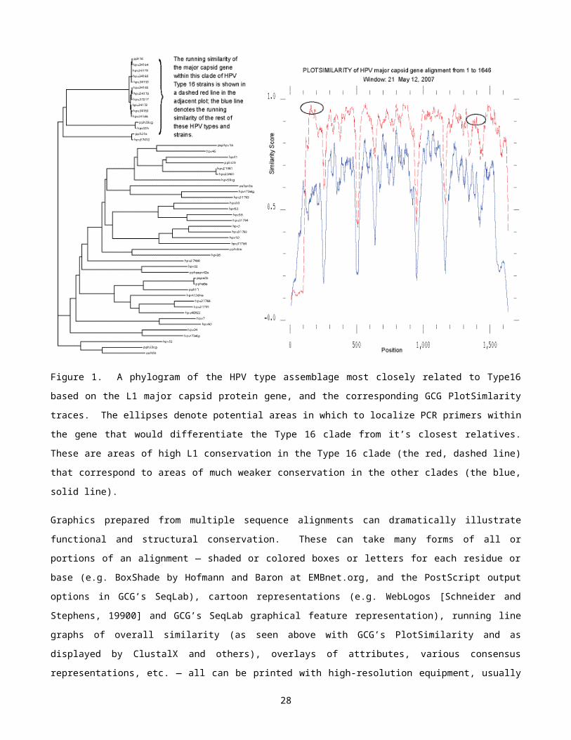
would like, it would probably be prudent to arbitrarily trim the dataset down from the 52 sequences present to

something more manageable. You can easily do this by selecting entries and then using the “Edit” menu “Delete

sequence(s)” function. Toggle the display back to DNA by unchecking the “Props” menu “View as protein”

checkbox, and notice that all gaps are in multiples of three, as it needs to be in a protein coding DNA alignment.

Return the alignment to protein visualization.

Even though this dataset aligns so easily, let’s experiment with MAFFT through SeaView so you can see how the

GUI deals with external methods. The “Props” menu “Alignment options” “Edit options” choice allows you to

modify the default parameters for whatever alignment method is checked, and “Add external method” allows you

to build commands for methods other than ClustalW and Muscle (however, if you downloaded my sample

configuration file you’ll have ten choices already there, though the paths may be incorrect, and you may not have

T-Coffee installed). Pick “Alignment options” “Add external method” so that we can add MAFFT to the default

choices. This will launch an “alignment method creation” box; hold your mouse cursor over the “Name” and

then the “Arguments” fields to see contextual help on the required syntax rules for adding external methods. If

MAFFT is in your system’s “$PATH,” you can just type “mafft” into the “Name” field, otherwise type in the full

path and the program name, or use the “Select external program” button and file chooser window. Type “--auto

%f.pir > %f.out” in the “Arguments” field to run MAFFT in its automatic mode that attempts to use the most

appropriate options for your particular dataset. Press the “alignment method creation” “OK” checkbox to save

the new method. Notice that the “Props” menu “Alignment options” choice now includes MAFFT; select it as

your new preferred method. Now use the “Edit” menu to “Align all sequences” with MAFFT. Check out the

screen log in your terminal window; it tells you what MAFFT is doing. Take note of the mode it chose. Load your

new alignment into the editor, and see if you can spot any differences. The results should be very similar to the

Muscle alignment. MAFFT chose its LINSI iterative refinement mode in my Linux environment based on the fact

that the dataset is fairly small and now consists of amino acids. What mode did it use for you? Figure 5 on the

following page shows a screen snapshot of my L1 protein LINSI alignment.

28

Figure 5. The SeaView graphical user interface editor window with an aligned HPV Li protein dataset loaded.

Switch back to DNA display, rerun MAFFT, and load these new results. This time MAFFT ran even faster for me,

since this time, at least with my Linux box, it choose FFTNSI. Is that what it did for you? Do you think the results

are as good as with the protein? They shouldn’t be, although this is pretty easy data. One thing that you should

probably know is SeaView totally starts fresh each time you make a complete new alignment. That is, it strips all

of the gaps that were there and starts all over each time. That’s probably enough for now with the simple dataset

example. Save your L1 alignment, if you are interested in keeping it around.

Let’s see how SeaView and MAFFT deal with the much tougher case of genomic data next. Use the “ File” menu

“Open” command to load “HPV_genome.fsa.” You’ll have two SeaView editor windows now. “Close” the L1

dataset window to leave the genome window by itself. If you didn’t save your previous alignment, you’ll be asked

whether you really want to close the window. Switch your display to visualize the corresponding protein

sequences with “Props” “View as protein” — check out all the asterisks! This data isn’t all in the same frame,

it’s not just coding sequence, it contains intergenic spacers, and it even has overlapping frames on some genes,

so there’s no way to align this dataset on the basis of its amino acids with these techniques. Therefore, we’re

stuck with the DNA. Switch back to see the DNA bases. Let’s see how well MAFFT works with them. Be sure

that your “Props” menu “Alignment options” still specifies MAFFT. Remember, we built this external method

with the “--auto” option, so MAFFT should be able to figure out what strategy will work best. < Double-click >

an entry to select them all and then use the “Edit” “Align all sequences” function to launch MAFFT on the

genomic data. This step will take a while, and if it’s just taking way too long, you may want to interrupt it and

reduce the number of sequences in the dataset, and then try it again.

MAFFT’s auto mode chose FFTNSI for my initial genomic analysis. After loading and scrolling through the

results, it’s apparent that some regions were found to align quite well, while other areas display no apparent

29

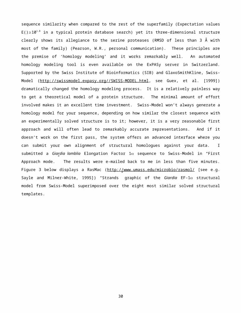
homology at all. At least some parts do look really good, even if the borders are a bit fuzzy. Figure 6 illustrates

one of these fuzzy borders, but also clearly displays correct alignment, since interior gaps are all in multiples of

three and the columns of color are undeniable.

Figure 6. A SeaView DNA display of a region within the HPV genome

where the E2 and E4 genes have overlapping reading frames.

This is the type of data that the

MAFFT EINSI strategy is built for,

although it is one of MAFFT’s

slowest modes. Nonetheless, I’ll

give it a try. If you grabbed one of

my sample SeaView configuration

files, then EINSI is already one of

your menu options. If not, then go

to the “Props” menu “Alignment options” “Add external method”

function, to add EINSI to your list of

SeaView alignment methods. Type

“einsi” into the “Name” field

(assuming MAFFT is in your path, or

specify the full path, or use “Select

external program”) and type

“%f.pir > %f.out” in the

“Arguments” field to run MAFFT in

its EINSI mode, that attempts to

align multiple alignable domains

embedded in the same order within

sequences otherwise not alignable.

Press the “alignment method creation” “OK” checkbox to save

the new method.

Next, you could use the “Props” menu “Alignment options” menu to select EINSI as your new preferred method,

and then “Edit” “Align all sequences” would align the data with MAFFT EINSI. Unfortunately, unless you have a

really, really fast computer, this step will take an extraordinary amount of time to finish, because EINSI is really

slow (but very accurate), and you’ll probably end up killing it. I let mine run to completion on our high performance

Linux server; it took a couple of hours! Regardless, EINSI is a great mode, good to have in your SeaView

alignment menu, because it works really well on smaller datasets of this nature, for example G-protein coupled

receptors, or RNA polymerases, which both have highly conserved domains strung along nearly unalignable

spacer sequence. This is especially true if you base your alignment on the protein sequences rather than on the

corresponding DNA sequences, for all the reasons already discussed. However, it works pretty well for things like

30

small subunit ribosomal RNA (SSU rRNA) too, since the individual domains of SSU rRNA are so well conserved.

And, if you expect huge gaps between the domains, then you can also use the “--ep 0” option.

So what are we going to do? How can we ‘clean up’ those ‘bad’ spots in our alignment? This is where the

concept of regional realignment can be a big help. Several interfaces, including SeaView, as well as GCG’s

SeqLab, GDE, and even ClustalX have the ability to select and work on just portions of an alignment. In SeaView

this, as well as the previously mentioned masking concepts, is done through the “Sites” menu. Use the “Sites“

menu to “Create set,” and give your new sites set an appropriate name. A new sequence line in white will appear

at the bottom of your data, and the display will ‘gray’ out. Now find a region of the alignment that you would like to

try to improve. < Click > on the left-hand, upstream end of the sites sequence under that region, and then find

the right-hand, downstream end of the ‘bad’ region and < control-click > on the sites sequence under it. A line of

“X”’s will appear delineating the region, and the region’s shading will return to normal. Be sure that you only have

that region selected; otherwise the subsequent regional realignment step won’t work, and you’ll just get an error

message. If you do have more than one block of sites selected either < shift-click > all of them except the one

you want, or, perhaps easier, just use “Sites” “Delete set” on the line and start over. Use “Sites” “Save set” to

preserve your work. You can have as many sites sets as you want. That way you can have one sites set

sequence for each region that you are interested in trying to realign.

Be sure that all of your sequences are still selected (< double-click > an entry name, if not) and then specify your

new EINSI method from your SeaView “Props” “Alignment options” menu. Next, launch EINSI on that region

with “Edit” “Align selection.” A new window will appear asking you to choose a “Reference Sequence.” This

will be that sequence in which the original gaps will be preserved and propagated into the subsequent alignment.

It doesn’t make much difference when you are realigning all of the sequences of a region, but it can be a big help

if you are trying to bring new sequences into an existing alignment, without using HMM or traditional profile

techniques or starting all over each time (also see MAFFT’s various profile options). If this is the case, select all

of your new sequences and just one of the previously aligned sequences as the reference, and then run your

desired alignment program on the full length of the dataset. I’ll pick PPH16 as my reference sequence, and the

program will start working on that region of the alignment. Running EINSI on a small bit of an alignment like this

versus the entire thing is very fast.

Accept the results of your realignment procedure and check it out. Note the strong columns of color. These

homologies may not be real, but at least if there are any recoverable homologies in that region, it seems like this

procedure has a lot better chance of capturing them than the previous alignment step. Regional realignment can

leave columns of gaps in your alignment, so go to the “Edit” menu and “Delete gap-only sites.” Figure 7 shows

my HPV genome alignment E2/E4 gene region just downstream from that in Figure 6, after I refined it with EINSI.

31

Figure 7. The HPV E2 E4 gene reading frame overlap region after EINSI refinement.

As in all computing, now would be a good time to “File” “Save as,” just in case. Obviously the overall objective

would be to go through your entire alignment and refine, maybe with EINSI, as much as possible, all of those

regions that you deem less than satisfactory. However, since you can only do one region at a time per sites set,

you either need to “Hide” and “Create” a new sites set (best), or “Delete” and “Create” and new set, or deselect all

of the previously selected sites each time, and then, regardless of how you’re doing it, select new sites to

delineate the new region that you would like to refine. Be sure to “Sites” “Save set” each time you create or

modify a sites set. And then, after you’ve exhausted this resource, if you really care, as I stress in the

introduction, you should use an appropriate editor like SeaView, to manually adjust things that you recognize as

just being wrong. In so many ways our own brain is still better at pattern recognition than any computer.

Another really neat thing that SeaView allows you to do, and that NEXUS and MASE format can contain (as well

as many others such as GCG’s RSF, but no others that SeaView can read/write) is to create feature annotation

for your alignment. In an alignment like this HPV genome dataset, that could be an incredibly helpful thing to

have. For instance you could indicate exactly where in the alignment each gene lies, or where various regulatory

elements occur. In protein alignments it is very helpful to annotate secondary structure, motifs, and active sites.

And if features overlap, you can have more than one footer line. Go to the “Footers” menu and “Create footer.” Give your footer an appropriate name. Now click the footer’s name in the editor and place your cursor where you

wish to add the annotation. Type whatever characters you wish. Another click on the footer’s name will disable

further editing of the line. I show an example in Figure 8 on the following page, where I indicate the poorly aligned

region that contains the downstream polyA signal of the two within the HPV genome.

32

Figure 8. The 3’ polyA signal of the HPV genome.

After you’ve got an alignment “as good as it’s ‘gonna’

get,” you can use sites sets in somewhat the opposite

way from above to export your desired format. Now

instead of delineating the ‘bad’ regions to try to

improve them, you will make a new sites set that

delineates all of the ‘good’ regions that will export into

a new file. This is the ‘masking’ concept that I keep

talking about; you mask away the unwanted regions,

by not including them in your sites set. And now you

do want to have multiple regions selected — all of

those regions in which you are confident of the

positional homology of the residues within it. When

you have your new sites set visible, and you “File”

“Save selection” and give your file a new and

appropriate name, then only those positions marked

by the “X”’s will be exported to your specified format.

However, if you use “File” “Save as” “NEXUS” or

MASE format (and give the new file a different,

appropriate name) then the output will include the

entire alignment, along with a section that specifies

your sites sets (CHARSET in a NEXUS format SETS

block).

The “Species” menu works similarly. Select your desired sequences and then use “Create group” to make

species sets. You can either save selected sequences with “File” “Save selection,” or, if you use NEXUS or

MASE format, you can save species sets (TAXSET in a NEXUS format SETS block) with “File” “Save as.” And,

like sites sets, you can have multiple species sets. Furthermore, you can combine sites sets and species sets to

export only particular regions of particular sequences!

Conclusion

The comparative method is a cornerstone of the biological sciences, and key to understanding much of life in so

many ways. Multiple sequence alignment is the comparative method on a molecular scale, and is a vital

prerequisite to some of the most powerful biocomputing analyses available, such as structure/function prediction

and phylogenetic inference. Understanding something about the algorithms and the program parameters of

multiple sequence alignment is the only way to rationally know what is appropriate. Knowing and staying well

within the limitations of any particular method will avert a lot of frustration. Furthermore, realize that program

defaults may not always be appropriate. Think about what these default values imply and adjust them

accordingly, especially if the results seem inappropriate after running through a first pass with the default

33

parameters intact. Consistency based approaches, as seen in T-Coffee and with MAFFT’s slower modes can

help with these decisions.

Gunnar von Heijne in his quite readable but well dated treatise, Sequence Analysis in Molecular Biology;

Treasure Trove or Trivial Pursuit (1987), provides an appropriate conclusion:

“Think about what you’re doing; use your knowledge of the molecular system involved to guide

both your interpretation of results and your direction of inquiry; use as much information as

possible; and do not blindly accept everything the computer offers you . . . . Don’t expect your

computer to tell you the truth . . . if any lesson is to be drawn . . . it surely is that to be able to

make a useful contribution one must first and foremost be a biologist, and only second a

theoretician . . . . We have to develop better algorithms, we have to find ways to cope with the

massive amounts of data, and above all we have to become better biologists. But that’s all it

takes.”

Oftentimes, in ‘real life,’ you’ll need to deal with quite complicated datasets that will make you think — distantly

related local domains, perhaps not even in syntenic order between sequences; or widely divergent paralogous

systems resulting from large gene expansions; or extremely large sequence collections with megabases of

genomic data; often you’ll even need to resort to manual alignment, at least in some regions — these are the

situations that will present vexing alignment problems and difficult editing decisions. These are the times that a

comprehensive multiple sequence editor such as SeaView can be of tremendous help.

References

Altschul, S.F., Gish, W., Miller, W., Myers, E. W., and Lipman, D. J. (1990) Basic Local Alignment Tool. Journal of

Molecular Biology 215, 403–410.

Altschul, S.F., Madden, T.L., Schaffer, A.A., Zhang, J., Zhang, Z., Miller, W., and Lipman, D.J. (1997) Gapped

BLAST and PSI-BLAST: a new generation of protein database search programs. Nucleic Acids Research 25,

3389–3402. Server at http://www.ncbi.nlm.nih.gov/BLAST/, and source code at ftp://ftp.ncbi.nih.gov/blast/.

Bailey, T.L. and Elkan, C., (1994) Fitting a mixture model by expectation maximization to discover motifs in

biopolymers, in Proceedings of the Second International Conference on Intelligent Systems for Molecular

Biology, AAAI Press, Menlo Park, California, U.S.A. pp. 28–36.

Bailey, T.L. and Gribskov, M. (1998) Combining evidence using p-values: application to sequence homology

searches. Bioinformatics 14, 48–4.

Bairoch A. (1992) PROSITE: A Dictionary of Sites and Patterns in Proteins. Nucleic Acids Research 20, 2013–

2018.

Bininda-Emonds, O.R.P. (2005) transAlign: using amino acids to facilitate the multiple alignment of protein-coding

DNA sequences. BioMed Central Bioinformatics 6, 156. Available through

http://www.personal.uni-jena.de/~b6biol2/ProgramsMain.html.

34

Clamp, M., Cuff, J., Searle, S. M. and Barton, G. J. (2004), The Jalview Java Alignment Editor, Bioinformatics 20,

426–427. Available at http://www.jalview.org/.

Cole, J.R., Chai, B., Farris, R.J., Wang, Q., Kulam-Syed-Mohideen, A.S., McGarrell, D.M., Bandela, A.M.,

Cardenas, E., Garrity, G.M., and Tiedje, J.M. (2007) The ribosomal database project (RDP-II): Introducing

myRDP space and quality controlled public data. Nucleic Acids Research 35,169–172. See

http://rdp.cme.msu.edu/.

Do, C.B., Mahabhashyam, M.S.P., Brudno, M., and Batzoglou, S. (2005) ProbCons: Probabilistic Consistency-

based multiple sequence alignment. Genome Research 15, 330-340. Available at

http://probcons.stanford.edu/download.html.

Eddy, S.R. (1996) Hidden Markov models. Current Opinion in Structural Biology 6, 361–365.

Eddy, S.R. (1998) Profile hidden Markov models. Bioinformatics 14, 755–763.

Edgar, R.C. (2004) MUSCLE: multiple sequence alignment with high accuracy and high throughput. Nucleic Acids

Research 32, 1792-1797. Available through http://www.drive5.com/muscle/.

Edgar, R.C. and Batzoglou, S. (2006) Multiple sequence alignment. Current Opinion in Structural Biology 16,

368–373.

Etzold, T. and Argos, P. (1993) SRS — an indexing and retrieval tool for flat file data libraries. Computer

Applications in the Biosciences 9, 49–57.

Felsenstein, J. (1980-2009) PHYLIP (Phylogeny Inference Package) version 3.6. Distributed by the author.

Department of Genome Sciences, University of Washington, Seattle, Washington, U.S.A. Available at

http://evolution.genetics.washington.edu/phylip.html.

Feng, D.F. and Doolittle, R. F. (1987) Progressive sequence alignment as a prerequisite to correct phylogenetic

trees. Journal of Molecular Evolution 25, 351–360.

Galtier, N., Gouy, M. and Gautier, C. (1996) SeaView and Phylo_win, two graphic tools for sequence alignment

and molecular phylogeny. Compututer Applications in the Biosciences 12, 543–548. Available through

http://pbil.univ-lyon1.fr/software/.

Gascuel, O. (1997) BIONJ: an improved version of the NJ algorithm based on a simple model of sequence data.

Molecular Biology and Evolution 14,685–695. Available at http://www.atgc-montpellier.fr/bionj/.

Genetics Computer Group (GCG), (Copyright 1982-2007) Program Manual for the Wisconsin Package, version

11, A ‘retired’ subsidiary of Accelrys, Inc., San Diego, California, U.S.A.

Gilbert, D.G. (1990–2006) ReadSeq. Distributed by the author. Biology Department, Indiana University,

Bloomington, Indiana, U.S.A. See http://iubio.bio.indiana.edu/soft/molbio/readseq/.

35

Gonnet, G.H., Cohen, M.A., and Benner, S.A. (1992) Exhaustive matching of the entire protein sequence

database. Science 256, 1443–1145.

Gotoh, O. (1982) An improved algorithm for matching biological sequences. Journal of Molecular Biology 162,

705–708.

Gribskov, M., McLachlan, M., and Eisenberg, D. (1987) Profile analysis: detection of distantly related proteins.

Proceedings of the National Academy of Sciences U.S.A. 84, 4355–4358.

Gupta, S.K., Kececioglu, J.D., and Schaffer, A.A. (1995) Improving the practical space and time efficiency of the

shortest-paths approach to sum-of-pairs multiple sequence alignment. Journal of Computational Biology 2,

459–472. MSA available at http://www.ncbi.nlm.nih.gov/CBBresearch/Schaffer/msa.html.

Guex, N., Diemand, A., and Peitsch, M.C. (1999) Protein modelling for all. Trends in the Biochemical Sciences

24,364–367. See http://swissmodel.expasy.org//SWISS-MODEL.html

Guindon S. and Gascuel O. (2003) A simple, fast, and accurate algorithm to estimate large phylogenies by

maximum likelihood. Systematic Biology 52, 696–704.

Henikoff, S. and Henikoff, J.G. (1992) Amino acid substitution matrices from protein blocks. Proceedings of the

National Academy of Sciences U.S.A. 89, 10915–10919.

Higgins, D.G., Bleasby, A.J., and Fuchs, R. (1992) CLUSTALV: improved software for multiple sequence

alignment. Computer Applications in the Biological Sciences 8, 189–191.

Hofmann, K. and Baron, M. (1999) BOXSHADE server at http://www.ch.embnet.org/software/BOX_form.html;

software available at ftp://www.isrec.isb-sib.ch/pub/boxshade.

Karlin, S. and Altschul, S.F. (1990) Methods for assessing the statistical significance of molecular sequence

features by using general scoring schemes. Proceedings of the National Academy of Sciences U.S.A. 87,

2264–2268.

Katoh, K., Misawa, K., Kuma, K., and Miyata T. (2002) MAFFT: a novel method for rapid multiple sequence

alignment based on fast Fourier transform. Nucleic Acids Research 30, 3059–3066.

Katoh, K., Kuma, K., Toh, H., and Miyata T. (2005) MAFFT version 5: improvement in accuracy of multiple

sequence alignment. Nucleic Acids Research 33, 511–518. Available at

http://align.bmr.kyushu-u.ac.jp/mafft/software/.

Letondal, C. and Schuerer, K. Pasteur Institute, Paris, France, http://www.pasteur.fr/english.html. ProtAl2DNA

available at ftp://ftp.pasteur.fr/pub/GenSoft/unix/alignment/protal2dna.

Lunter, G., Miklos, I., Drummond, A., Jensen, J.L., and Hein, J. (2005) Bayesian coestimation of phylogeny and

sequence alignment. BioMed Central Bioinformatics 6, 83

36

National Center for Biotechnology Information (NCBI) Entrez, public domain software distributed by the authors.

http://www.ncbi.nlm.nih.gov/Entrez/ National Library of Medicine, National Institutes of Health, Bethesda,

Maryland, U.S.A.

Needleman, S.B. and Wunsch, C.D. (1970) A general method applicable to the search for similarities in the amino

acid sequence of two proteins. Journal of Molecular Biology 48, 443–453.

Notredame, C. (2006) T-Coffee: Tutorial and FAQ and Technical Documentation. Included with the distribution

through http://www.tcoffee.org/Projects_home_page/t_coffee_home_page.html.

Notredame, C., Higgins, D.G., and Heringa, J. (2000) T-Coffee: a novel method for multiple sequence alignments.

Journal of Molecular Biology 302, 205-217.

Olsen, G. (1992) lecture: Inference of Molecular Phylogenies, University of Illinois at Urbana-Champaign, U.S.A.;

Thursday, September 3, 1992.

Pearson, W.R. (1990) Rapid and sensitive sequence comparison with FASTP and FASTA. Methods in

Enzymology 183, 63–98.

Pearson, W.R. (1998) Empirical statistical estimates for sequence similarity searches. Journal of Molecular

Biology 276, 71–84. The complete FastA package is available through

http://fasta.bioch.virginia.edu/fasta_www2/fasta_down.shtml.

Pearson, W.R. and Lipman, D.J. (1988) Improved tools for biological sequence analysis. Proceedings of the

National Academy of Sciences U.S.A. 85, 2444–2448.

Rambaut, A. (1996) Se-Al: Sequence Alignment Editor. Available at http://evolve.zoo.ox.ac.uk/ software.html?

id=seal.

Rice, P., Longden, I. and Bleasby, A. (2000) EMBOSS: The European Molecular Biology Open Software Suite

Trends in Genetics 16, 276–277. Available at http://emboss.sourceforge.net/.

Ronquist, F. and Huelsenbeck, J.P. (2003) MRBAYES 3: Bayesian phylogenetic inference under mixed models.

Bioinformatics 19,1572–1574. See http://mrbayes.scs.fsu.edu/.

Rozen, S. and Skaletsky, H. (2000) Primer3 on the WWW for general users and for biologist programmers. In:

Krawetz, S. and Misener, S. (eds) Bioinformatics Methods and Protocols: Methods in Molecular Biology.

Humana Press, Totowa, NJ, pp 365-386. Available at http://primer3.sourceforge.net/.

Saitou, N. and Nei, M. (1987) The Neighbor-Joining Method: A New Method of Constructing Phylogenetic Trees.

Molecular Biology and Evolution 4, 1406–1425.

Sayle, R.A. and Milner-White, E.J. (1995) RasMol: Biomolecular graphics for all. Trends in the Biochemical

Sciences 20,374–376. See http://www.umass.edu/microbio/rasmol/ and http://openrasmol.org/.

37

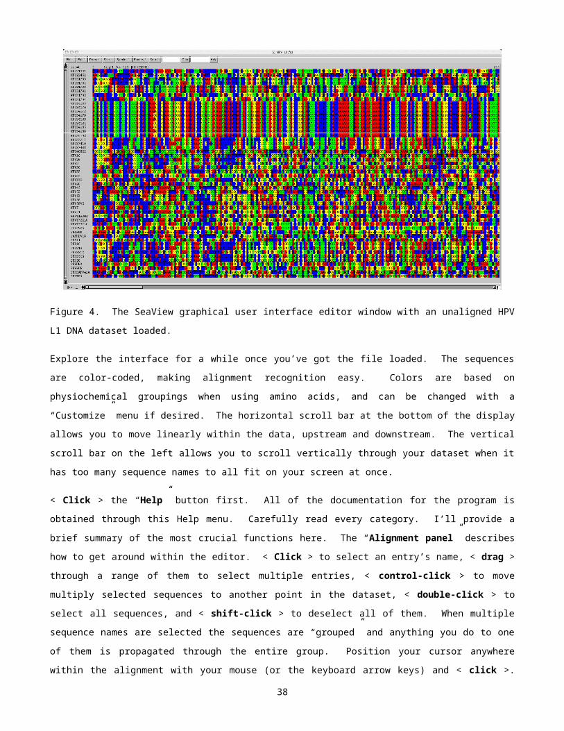
Schneider, T.D. and Stephens, R.M. (1990) Sequence logos: A new way to display consensus sequences.

Nucleic Acids Research 18, 6097-6100. See http://www-lmmb.ncifcrf.gov/~toms/sequencelogo.html.

Schwartz, R.M. and Dayhoff, M.O. (1979) Matrices for detecting distant relationships, in Atlas of Protein

Sequences and Structure (Dayhoff, M.O. ed.) 5, National Biomedical Research Foundation, Washington,

D.C., U.S.A. pp. 353–358.

Smith, R.F. and Smith, T.F. (1992) Pattern-induced multi-sequence alignment (PIMA) algorithm employing

secondary structure-dependent gap penalties for comparative protein modeling. Protein Engineering 5, 35–

41. Available at http://genamics.com/software/downloads/pima-1.40.tar.gz.

Smith, R.F., Wiese, B.A., Wojzynski, M.K., Davison, D.B., Worley, K.C. (1996) BCM Search Launcher — an

integrated interface to molecular biology data base search and analysis services available on the World Wide

Web. Genome Research 6, 454–62. See http://searchlauncher.bcm.tmc.edu/.

Smith, S.W., Overbeek, R., Woese, C.R., Gilbert, W., and Gillevet, P.M. (1994) The Genetic Data Environment,

an expandable GUI for multiple sequence analysis. Computer Applications in the Biosciences 10, 671–675.

The original Sun OS version is at ftp://megasun.bch.umontreal.ca/pub/gde/. See Linux and Mac OS X GDE

ports at http://www.bioafrica.net/GDElinux/index.html and http://www.msu.edu/~lintone/macgde/.

Smith, T.F. and Waterman, M.S. (1981) Comparison of bio-sequences. Advances in Applied Mathematics 2, 482–

489.

Stajich, J.E., Block, D., Boulez, K., Brenner, S.E., Chervitz, S.A., Dagdigian, C., Fuellen, G., Gilbert, J.G., Korf, I.,

Lapp, H., Lehvaslaiho, H., Matsalla, C., Mungall, C.J., Osborne, B.I., Pocock, M.R., Schattner, P., Senger, M.,

Stein, L.D., Stupka, E., Wilkinson, M.D., and Birney, E. (2002) The Bioperl toolkit: Perl modules for the life

sciences. Genome Research 12, 1611–1618. Available at http://www.bioperl.org/.

Suyama, M., Torrents, D. and Bork P. (2006) PAL2NAL: robust conversion of protein sequence alignments into

the corresponding codon alignments. Nucleic Acids Research 34, 609–612. See http://coot.embl.de/pal2nal/.

Swofford, D.L. 1989–2007. PAUP* (Phylogenetic Analysis Using Parsimony, and other methods) version 4.0+.

Illinois Natural History Survey, 1994; personal copyright, 1997; Smithsonian Institution, Washington D.C.,

U.S.A., 1998; Florida State University, 2001–2007. Home page at http://paup.scs.fsu.edu/, distributed

through Sinaeur Associates, Inc. at http://www.sinauer.com/ Sunderland, Massachusetts, U.S.A.

Thompson, J.D., Gibson, T.J., Plewniak, F., Jeanmougin, F. and Higgins, D.G. (1997) The ClustalX windows

interface: flexible strategies for multiple sequence alignment aided by quality analysis tools. Nucleic Acids

Research 24, 4876–4882. Available at ftp://ftp-igbmc.u-strasbg.fr/pub/ClustalX/.

Thompson, J.D., Higgins, D.G. and Gibson, T.J. (1994) CLUSTALW: improving the sensitivity of progressive

multiple sequence alignment through sequence weighting, positions-specific gap penalties and weight matrix

choice. Nucleic Acids Research 22, 4673–4680. Available at http://www.ebi.ac.uk/clustalw/.

38

Van de Peer, Y., Frickey, T., Taylor, J.S. and Meyer, A. (2002) Dealing with saturation at the amino acid level: A

case study based on anciently duplicated zebrafish genes. Gene 295, 205–211. ASaturA available at

http://bioinformatics.psb.ugent.be/software_details.php?id=6.

von Heijne G. (1987) Sequence Analysis in Molecular Biology; Treasure Trove or Trivial Pursuit. Academic Press,

San Diego, California, U.S.A.

Waterman, M.S. (1989) Sequence alignments, in Mathematical Methods for DNA Sequences (Waterman, M.S.

ed.), CRC Press, Boca Raton, Florida, U.S.A.

Wernersson, R. and Pedersen A.G. (2003) RevTrans — Constructing alignments of coding DNA from aligned

amino acid sequences. Nucleic Acids Research 31, 3537–3539. Available at

http://www.cbs.dtu.dk/services/RevTrans/download.php.

Wuyts, J., Perriere, G., and Van de Peer, Y. (2004) The European ribosomal RNA database. Nucleic Acids

Research 32,101–103. See http://www.psb.ugent.be/rRNA/.

39